Analysis of Synchronous Generators’ Local Mode Eigenvalues in Modern Power Systems

Abstract

New energy sources, storage facilities, power electronics devices, advanced and complex control concepts, economic operating doctrines, and cost-optimized construction and production of machines and equipment in power systems adversely affect small-signal stability associated with local oscillations. The objective of the article is to analyze local oscillations and the causes that affect them in order to reduce their negative impact. There are no recognized analyses of the oscillations of modern operating synchronous generators exposed to new conditions in power systems. The basic idea is to perform a numerical analysis of local oscillations of a large number of synchronous generators in the power system. The paper represents the local mode data obtained from a systematic analysis of synchronous generators in the Slovenian power system. Analyzed were 74 synchronous generators of the Slovenian power system, plus many additional synchronous generators for which data were accessible in references. The mathematical models convenient for the study of local oscillations are described first in the paper. Next, the influences of transmission lines, size of the synchronous generators, operating conditions, and control systems were investigated. The paper’s merit is the applicable rules that have been defined to help power plant operators avoid stability-problematic situations. Consequently, boundaries were estimated of the eigenvalues of local modes. Finally, experiments were performed with a laboratory-size synchronous generator to assess the regularity of the numerically obtained conclusions. The obtained results enable the prediction of local oscillations’ frequencies and dampings and will be useful in PSS planning.

1. Introduction

1.1. Motivation, Current State, and Basics

As part of our regular work, we have to investigate in detail the small-signal stability of the Slovenian power system. Since small-signal stability is directly related to (and dependent on) local oscillation modes, we first conducted a detailed study of the local oscillations of synchronous generators in the Slovenian power system. Local oscillations are associated with examining the rotor angle oscillations of a single power plant against the rest of the power system [1]. Since the results obtained are universal and, we estimate, valuable for other power system operators and researchers, we present the results of this study in this paper. The following paragraphs summarize basic definitions and the current state of power system stability.

Power system stability is the ability of an electric power system, for a given initial operating condition, to regain a state of operating equilibrium after being subjected to a physical disturbance, with most system variables bounded, so that practically the entire system remains intact [1]. Disturbances can be divided into small ones, which represent a continually changing load, and larger ones, such as unexpected failures and switching.

The essential elements of power systems are synchronous generators. In recent decades, we have witnessed a significant increase in the stability problems of many synchronous generators operating in the power system. There are three main reasons for that:

-

Changes in the construction of synchronous generators, which come from cost optimization requirements for production and transport of the generators. Consequently, the damping coefficients of the rotor’s damping windings and inertia moments are reduced [2].

-

Introduction of additional control systems into power systems or their modification, which is inevitable due to altered modes of operation of the power systems (e.g., operation of facilities at their peak performance); reaching novel, strict requirements of transmission system operators; open transmission access; environmental constraints; and increased competitiveness (e.g., additional voltage control systems which are suggested by transmission system operators (TSO) to control the power plant terminal voltage versus reactive power characteristics, modified primary control systems which will be able to assure the TSOs requirements during parallel operation, island operation of the single generators, and parallel operation of a few power-generating modules within one island). The additional or modified control systems improve operation in a particular operation regime. In some other operation conditions, the additional control systems could reduce damping and lead to instability of the power system [2].

-

As the demand for energy grows, modern power systems are operated close to the ultimate transmission capability, which can easily lead to a critical situation [3].

For these reasons, synchronous generators in modern power systems are much more sensitive to disturbances in the power system (damages, faults, errors) that cause natural oscillations to become unstable.

Consequences of elevated stability problems are observed clearly in an increasing number of significant power system blackouts in recent years. Due to their importance, there are many reviews in the literature, e.g., [3]. It can be seen that the highest number of blackouts was due to abnormal weather conditions, such as severe winds and heavy storms, and trees falling on transmission lines. These were the reasons for about 50% of all outages in the world in 2011–2019. Faulty equipment and human error are in second place as reasons for blackouts. In the same time period, these were the reasons for about 31.8% of all global blackouts. From [3], it is evident that, in 2011, there were about 2050 blackouts, which lasted an average of 4 h. The data collected show that blackouts have an extraordinarily negative impact on modern society and cause significant economic damage.

The instability of power systems can take different forms and can be influenced by a wide range of factors. According to [3], local oscillation modes and small-signal stability are inherently connected to rotor angle stability.

Rotor angle stability refers to the ability of synchronous machines of an interconnected power system to remain in synchronism after being subjected to a disturbance. The rotor angle stability problem involves the study of the electromechanical oscillations inherent in power systems. For convenience in analysis and for gaining useful insight into the nature of stability problems, it is useful to classify rotor angle stability in two subcategories: small-signal rotor angle stability (or small-signal, steady-state, small-disturbance, long-term, or dynamic (in the USA) stability) and large-signal rotor angle stability (or large-signal, transient, short-term, or dynamic (in Europe) stability).

Small-signal stability is concerned with the ability of the power system to maintain synchronism under small disturbances. The disturbances are considered to be sufficiently small that linearization of system equations is permissible for purposes of analysis [3]. The instability that may result can be of two forms: an increase in rotor angle through a non-oscillatory (aperiodic) mode due to lack of synchronizing torque, or rotor oscillations of increasing amplitude due to lack of sufficient damping torque. In today’s power systems, a small-signal stability problem is usually associated with insufficient damping of oscillations. The aperiodic instability problem has been largely eliminated by the use of continuously acting automatic voltage regulators (AVR) [3].

Synchronous generator oscillations are the main reason for problems concerning small-signal stability. Oscillations occur between the synchronous generator and some other parts of the power system. According to the elements between which oscillations occur, we arrange these oscillations in five classes: between a single synchronous generator against the rest of the power system (called local oscillation modes, local oscillations, local modes, machine-system modes, or single-machine infinite-bus oscillations), between the rotors of a few generators close to each other (inter-machine or interplant oscillation modes), between synchronous generators against a turbine (torsional oscillation modes), between different parts of the power plant due to the interaction of control systems (control oscillation modes), and between a group of generators in one area against a group of generators in another area (inter-area oscillation modes). Most frequently encountered small-signal stability problems are from the class of local oscillation modes [4]. This is the reason why the detailed results of the research of local modes are presented in the article.

1.2. Limitations and Aims of This Work

The paper is focused on a detailed investigation of local oscillation modes. The presented work is related to the study of oscillations in the Slovenian power system. The Slovenian power system covers a small area (20,271 km²) and has strong 400-kV transmissions between the country and neighboring countries. It has 74 synchronous generators with nominal power >1 MVA. The majority of generators are of small nominal power (between 10 and 40 MVA); only two generators are large (813 MVA in the nuclear power plant and 727 MVA in the thermal power plant). Due to most small and well-distributed generators and their direct connections (over block transformers and relatively short transmission lines) to the stiff backbone, the local oscillation modes are pronounced in the Slovenian power system.

In this paper, we have tried to answer the following questions:

-

What are the frequencies and dampings of local oscillations for different generators? Can we estimate the area where the eigenvalues of local oscillation modes for other generators lie?

-

How does the generator’s operating point (i.e., its active and reactive power) affect its local mode eigenvalues? Is this effect similar for different generators (size, age, type)? What impact does the connection to the infinite bus have?

-

What is the impact of control systems on local mode eigenvalues?

The purpose of the obtained findings will be:

-

The prognosis (estimation) of the local oscillations without measurement.

-

In the case of available measured data of existent oscillations (instantaneous values of produced three-phase powers and rotor speeds of generators), the classification of the measured oscillations in the local oscillations (and exclude them from torsional oscillations, control oscillations, and inter-area oscillations).

-

To prevent activities that would cause local mode eigenvalues to become stability-problematic.

-

To make these eigenvalues better damped (PSS design does not fall within the scope of this paper).

1.3. Existing Solutions and Literature Review

Synchronous generator oscillations are an important engineering problem and an interesting scientific challenge. Accordingly, there is great activity and a number of publications in this area.

An appropriate mathematical model is required to estimate and predict the characteristics of oscillations. A simplified linearized model of a single machine connected to an infinite bus (SMIB) is considered to be the fundamental model for the local oscillation analysis. The model was presented in [5] and named, according to the authors, the Heffron–Phillips model (H–P model). The H–P model was supplemented and changed constantly. This process is still ongoing, e.g., [6,7], but the fundamental H–P model is still considered the basis for research in this area. Analytical determination of H–P model parameters is described in detail in [4,8], along with the identification of the model’s parameters in [9,10].

The first articles that give a model-based quantitative assessment of the frequency of oscillation of synchronous generators are more than 20 years old. In [11], the author estimates that the control oscillation frequencies are in the range of 1.5–2.5 Hz, and the torsional oscillations are in the range of 10–50 Hz. In [12], it is estimated that the local oscillations are in the range of 0.8–1.8 Hz and the inter-area oscillations in the range of 0.2–0.5 Hz. These findings still apply to the indicative values. A broad overview of the sources, characteristics, and analyses of natural oscillatory behaviors in power systems is provided in [13]. Inter-area electromechanical modes in ambient response are considered explicitly in this report.

Although the constructions of synchronous generators, control concepts, and network connections have changed significantly over time, we do not find recent publications in the literature in which local oscillation frequencies are estimated based on the analysis of a large number of synchronous generators. An additional research gap is that there are no publications where the expected damping of these oscillations is evaluated in detail. A mode’s damping influences how quickly (and if) a related oscillation subsides. Therefore, damping is the parameter tied most closely to system stability [13]. The need for knowledge in this area is confirmed by recent publications that address the damping of oscillations resulting from new solutions and equipment according to synchronous generators. The damping of oscillations produced due to the introduction of a photovoltaics virtual synchronous generator is considered in [14]. Reference [15] studies the oscillations of wind farms’ synchronous generators. Reference [16] describes the implementation of an energy storage system for the damping of electromechanical oscillations of synchronous generators. References [17,18,19] describe the effects of control appliances on the power grid frequency, power system blackouts, and cascading failures. Reference [20] highlights the small-signal oscillations of a synchronous motor–generator pair, which are exposed and treated in more detail. It is just one of the articles that confirms the topicality of the considered matter.

1.4. Contribution and Paper Structure

We can display four original contributions of the paper:

-

An estimate is made of the expected local mode eigenvalues of synchronous operating generators (the boundaries of the areas where eigenvalues for different types of synchronous generators in different operating conditions are expected).

-

The impact of the operating point of synchronous generators on the local mode eigenvalue is investigated; defined are rules which help the operators to estimate under which operating conditions local oscillations are most weakly damped.

-

The impact of the AVR on the local oscillations is analyzed.

-

Experimental results, which are important because they confirm numerically obtained results.

The article is organized into six sections. The linearized mathematical model of a synchronous generator connected to the infinite bus is shown in the second section. An eigenvalue analysis for synchronous generators without a control system is presented in the third section. The impact of the AVR is studied in the fourth section. Some measurement results are shown in the fifth section. In conclusion, first, a summary of the most important results is given, and second, some topics are provided for future research in the field of synchronous generator oscillations.

2. Mathematical Model of a Synchronous Generator Connected to an Infinite Bus

Due to the extreme importance of synchronous generators, it is expected that the activities in the field of synchronous generator modeling have been, and still are, very intensive. There is a distinct interest in adequate static and dynamic models of synchronous generators. These models accelerate the design and the construction of synchronous generators, facilitate the analysis and simulation of synchronous generators’ operation, and enable the systematic synthesis of their control systems [8]. There are many models of different levels of complexity that are suitable for various qualitative and quantitative analyses of synchronous generators. The most fundamental model of a synchronous generator is the non-linear seventh-order dq model (NLM), where the magnetic coupling of stator, field, and damper windings is a function of the position and saturation of a rotor. For the analysis of electromechanical oscillations of a synchronous generator connected to a strong network, the generator model is supplemented with the simple lumped-parameters model of the transmission line between a synchronous generator and an infinite bus. This model certainly represents the best description of the dynamic and static behavior of a synchronous generator. The disadvantage of this model is the need to know a large number of the parameters of the synchronous generator. These parameters are mainly unknown and challenging to measure. Therefore, the use of this model is inappropriate in cases where a model-based quantitative analysis of a real synchronous generator is intended.

For the purposes of small-signal electromechanical oscillation analysis, the use of linearized synchronous generator models is satisfactory. They describe the synchronous generator’s dynamics in the proximity of the selected equilibrium point. Linearized models are characterized by the dependence of their parameters on the equilibrium point from which they are derived. By changing the synchronous generator’s operating point (i.e., equilibrium point), the parameters of the linearized models also change. Linearized models enable easy evaluation of eigenvalue analysis, which offers good insight into the frequency and damping of electromechanical oscillations.

Linearized models of different levels are known and used. Among many linearized models of different orders, the Heffron–Phillips model (H–P model) is the most popular. A detailed description of the assumptions regarding the development of this model, comparison of the H–P model with NLM, and the research of applicability of the H–P model in an entire operating range can be found in [8].

The H–P model has two inputs and three state-space variables. The inputs are mechanical torque deviation T_mΔ(t) and rotor winding voltage deviation E_fdΔ(t). The state-space variables are rotor angle deviation δ_Δ(t), rotor speed deviation ω_Δ(t), and voltage behind transient reactance deviation ${E^{\prime }}_{\mathrm{q}\mathsf{\Delta }}(t)$. Additional outputs are electric torque deviation T_eΔ(t) and terminal stator voltage deviation V_tΔ(t). All the inputs and the state-space variables denote the deviations (subscript _Δ) from the equilibrium state. The minimum set of the parameters and the operating point values of the synchronous generator, transmission line, and infinite bus necessary to calculate the H–P model’s parameters are presented in

Table 1. Data of synchronous generator and network for H–P model parameters calculation.

Parameters of Synchronous Generator	Ld (H), Lq (H), Ld’ (H), H (s), Re (Ω), Le (H), D (pu), Td0′(s)
Operating point quantities	P (W), Q (Var), ωs (rad s−1), V∞ (V)

.

The parameters L_d and L_q in

Table A1. Manufacturer’s data: hydro-type synchronous generator S_n = 9 MVA.

Sn = 9 [MVA]	Un = 6.9 [kV]	cos φn = 0.9	H = 2.61 [pu]
Ld = 0.911 [pu]	Lq = 0.580 [pu]	Ld′ = 0.408 [pu]	Ld″ = 0.329 [pu]
Rs = 0.03 [pu]	RF = 0.269 [pu]	Td0′= 4.20 [s]	D = 2 [pu]

are d- and q-axes inductances; L_d’ is d-axis transient inductance; H is an inertia constant; R_e and L_e are transmission line resistance and inductance; D is a damping coefficient representing total lumped damping effects; and T’_d0 is an open circuit time constant of a direct axis. The operating point values P and Q in Table A1 are active and reactive power at a machine terminal, respectively; ω_s is electric synchronous speed; and V_∞ is infinite bus voltage. From Table A1 can be seen the reduction of the parameters’ request of the H–P model compared to the NLM [8]. For calculation of the H–P model parameters, there is no need to know the synchronous generator’s d-axis sub-transient inductances; d- and q-axes leakage inductances; or stator, field, d-axis damping, and q-axis damping windings resistances.

From the data in Table 1, the auxiliary operating point variables’ values are calculated through synchronous machine phasor equations. The auxiliary operating point variables values in

Table 2. Auxiliary operating point variables necessary for calculation of the parameters of the H–P model.

Auxiliary operating point variables

δop, Vd,op, Vq,op, Id,op, Iq,op, Eop, E′q,op, Eqa,op

below must be determined before calculating the H–P model parameters.

The variables in Table 2: δ(t) is the electric rotor angle; V_d(t) and V_q(t) are stator terminal d- and q-axis voltages, respectively; I_d(t) and I_q(t) are the stator d- and q-axis currents, respectively; and E, E_qa, and E’_q are standardized phasor diagram EMFs. Index _op means an operating point value.

The H–P model is presented in a state-space form by (1) and (2) [8]. The linearization parameters K₁ to K₆ of the H–P model are calculated based on the values in Table A1 and

Table A2. Manufacturer’s data: hydro-type synchronous generator S_n = 12 MVA.

Sn = 12 [MVA]	Un = 6.9 [kV]	cos φn = 0.9	H = 9.08 [pu]
Ld = 0.970 [pu]	Lq = 0.700 [pu]	Ld′ = 0.350 [pu]	Ld″ = 0.315 [pu]
Rs = 0.033 [pu]	RF = 0.298 [pu]	Td0′= 3.8 [s]	D = 1.5 [pu]

[8]. All variables in the H–P model are normalized except electric rotor angle δ(t).

$$\left[\begin{array}{c}{\dot{\delta }}_{\mathsf{\Delta }}(t)\\ {\dot{\omega }}_{\mathsf{\Delta }}(t)\\ {{\dot{E}}^{\prime }}_{\mathrm{q}\mathsf{\Delta }}(t)\end{array}\right]=\left[\begin{array}{ccc}0& {\omega }_{\mathrm{s}}& 0\\ -\frac{K_1}{2H}& -\frac{D}{2H}& -\frac{K_2}{2H}\\ -\frac{K_4}{{T^{\prime }}_{\mathrm{d}0}}& 0& -\frac{1}{K_3{T^{\prime }}_{\mathrm{d}0}}\end{array}\right]\left[\begin{array}{c}{\delta }_{\mathsf{\Delta }}(t)\\ {\omega }_{\mathsf{\Delta }}(t)\\ {E^{\prime }}_{\mathrm{q}\mathsf{\Delta }}(t)\end{array}\right]+\left[\begin{array}{l}\begin{array}{cc}0& 0\\ \frac{1}{2H}& 0\end{array}\\ \begin{array}{cc}0& \frac{1}{{T^{\prime }}_{\mathrm{d}0}}\end{array}\end{array}\right]\left[\begin{array}{c}{T}_{\mathrm{m}\mathsf{\Delta }}(t)\\ E_{\mathrm{fd}\mathsf{\Delta }}(t)\end{array}\right]$$

(1)

$$\left[\begin{array}{c}{T}_{\mathrm{e}\mathsf{\Delta }}(t)\\ V_{\mathrm{t}\mathsf{\Delta }}(t)\end{array}\right]=\left[\begin{array}{l}\begin{array}{ccc}{K}_1& 0& K_2\end{array}\\ \begin{array}{ccc}{K}_5& 0& K_6\end{array}\end{array}\right]\left[\begin{array}{c}{\delta }_{\mathsf{\Delta }}(t)\\ {\omega }_{\mathsf{\Delta }}(t)\\ {E^{\prime }}_{\mathrm{q}\mathsf{\Delta }}(t)\end{array}\right]+\left[\begin{array}{cc}0& 0\\ 0& 0\end{array}\right]\left[\begin{array}{c}{T}_{\mathrm{m}\mathsf{\Delta }}(t)\\ E_{\mathrm{fd}\mathsf{\Delta }}(t)\end{array}\right]$$

(2)

The accuracy of the H–P model was investigated in [8]. Simulations with both NLM and H–P models were made and compared with experiments. The simulations and experiments were made systematically for different operating points in the entire operating range, as well as different dynamical changes of inputs (mechanical torque and excitation voltage). The high accordance of the H–P model is evident from the obtained results. Agreement in the first amplitude, the frequency, and the damping of the transient response is very high. The conclusion of [8] was that the H–P model describes synchronous generators’ electromechanical phenomena in the entire operating range in the case of the small input’s perturbations, which could be used for a detailed analysis of local oscillations.

3. Local Mode Analysis of Synchronous Generators without AVR

3.1. Eigenvalue Analysis

In the analysis, the turbo- and hydro-type synchronous generators with and without AVR system were considered separately. Due to the non-linearity and complexity of the analyzed plant, the fundamental mechanism analysis did not lead to useful conclusions, and especially not to quantitative results. Analytical treatment based on a linearized model proved to be too extensive and non-transparent. Experimental analysis (measurements) was not possible (allowed) for the majority of the power plants. Therefore, we used numerical eigenvalue analysis.

The assessment of local oscillations was performed on the basis of the analysis of the eigenvalues of the linearized H–P model. The linearized model of a synchronous generator has three eigenvalues, two complex conjugates and one real. The dominant complex conjugate eigenvalues are essential because they describe local oscillations. The real part and imaginary parts of the complex eigenvalues are related to the frequency and damping of the local oscillation.

To analyze the oscillations of synchronous generators, the eigenvalues λ₁, λ₂, and λ₃ were calculated by the characteristic Equation (3):

$$\begin{array}{l}\det (\lambda I-A)=0\to \\ 2K_{3}H{T^{\prime }}_{d0}\hspace{0.17em}{\lambda }^3+\left(K_{3}D{T^{\prime }}_{d0}+2H\right)\hspace{0.17em}{\lambda }^2+\left(K_1{K}_3{T^{\prime }}_{d0}{\omega }_{\mathrm{s}}+D\right)\hspace{0.17em}\lambda +\left(K_1{\omega }_{\mathrm{s}}-K_2{K}_3{K}_4{\omega }_{\mathrm{s}}\right)=0\end{array}$$

(3)

where A denotes the system matrix of the H–P state-space model in (1).

Dynamic mode e^σt sin(ωt + θ) corresponds to the complex eigenvalues λ_1,2 = σ ± j ω. The real part of eigenvalue σ determines the time constant of decay of the amplitude of the oscillations; in-1/σ seconds, the amplitude decays to 36.79% (i.e., e⁻¹ pu) of the initial amplitude (for a negative value of σ). The imaginary part of eigenvalues ω represents damped (or actual) frequency in rad/s. The eigenfrequency (or natural frequency) ω₀ and damping ratio ζ are given by:

$${\omega }_0=\sqrt{{\sigma }^2+{\omega }^2},\hspace{1em}\hspace{1em}\varsigma =\frac{-\sigma }{\sqrt{{\sigma }^2+{\omega }^2}}$$

(4)

3.2. Influence of Synchronous Generator’s Operating Point on Local Mode Eigenvalues

3.2.1. Hydro-Type Synchronous Generators

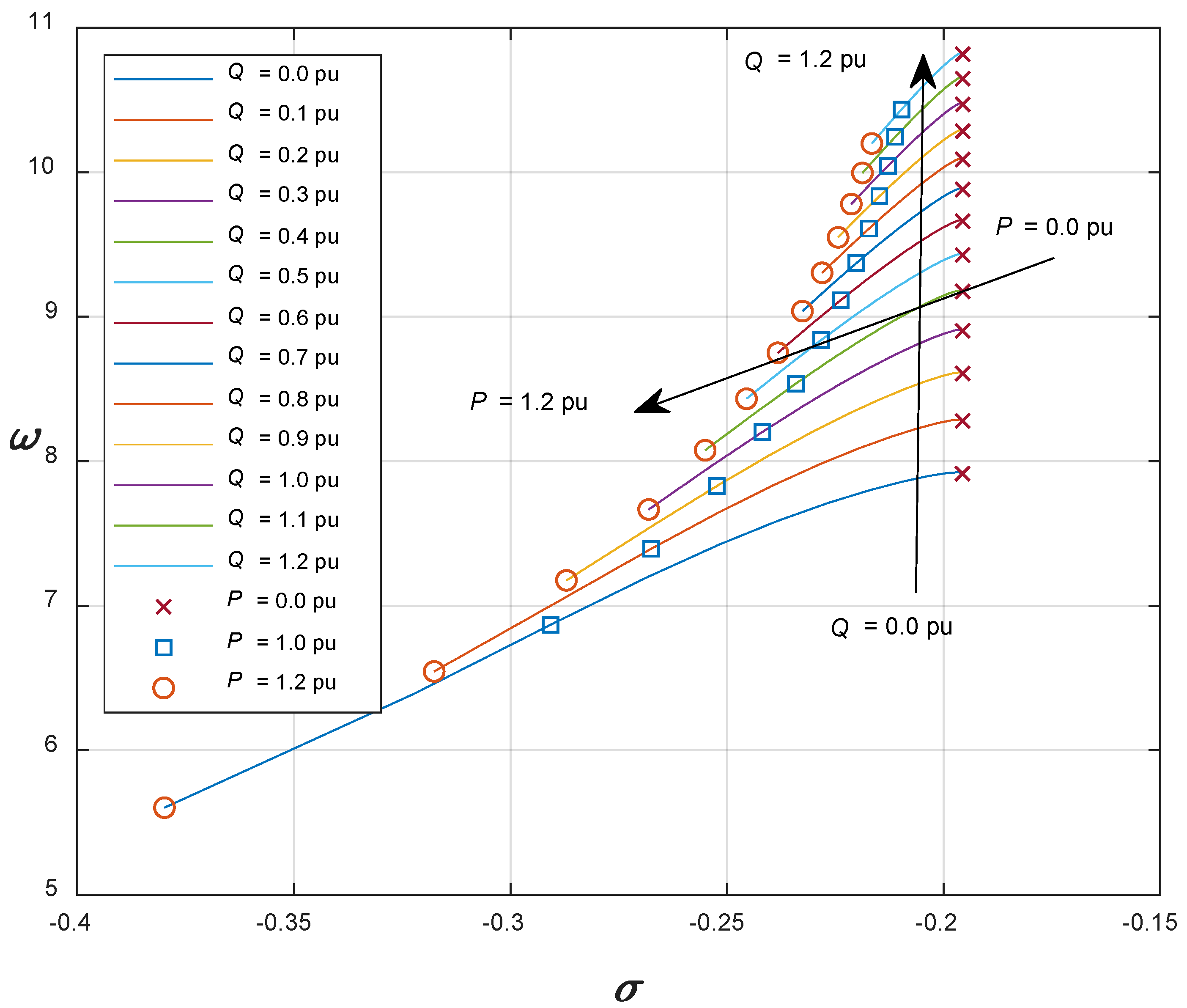
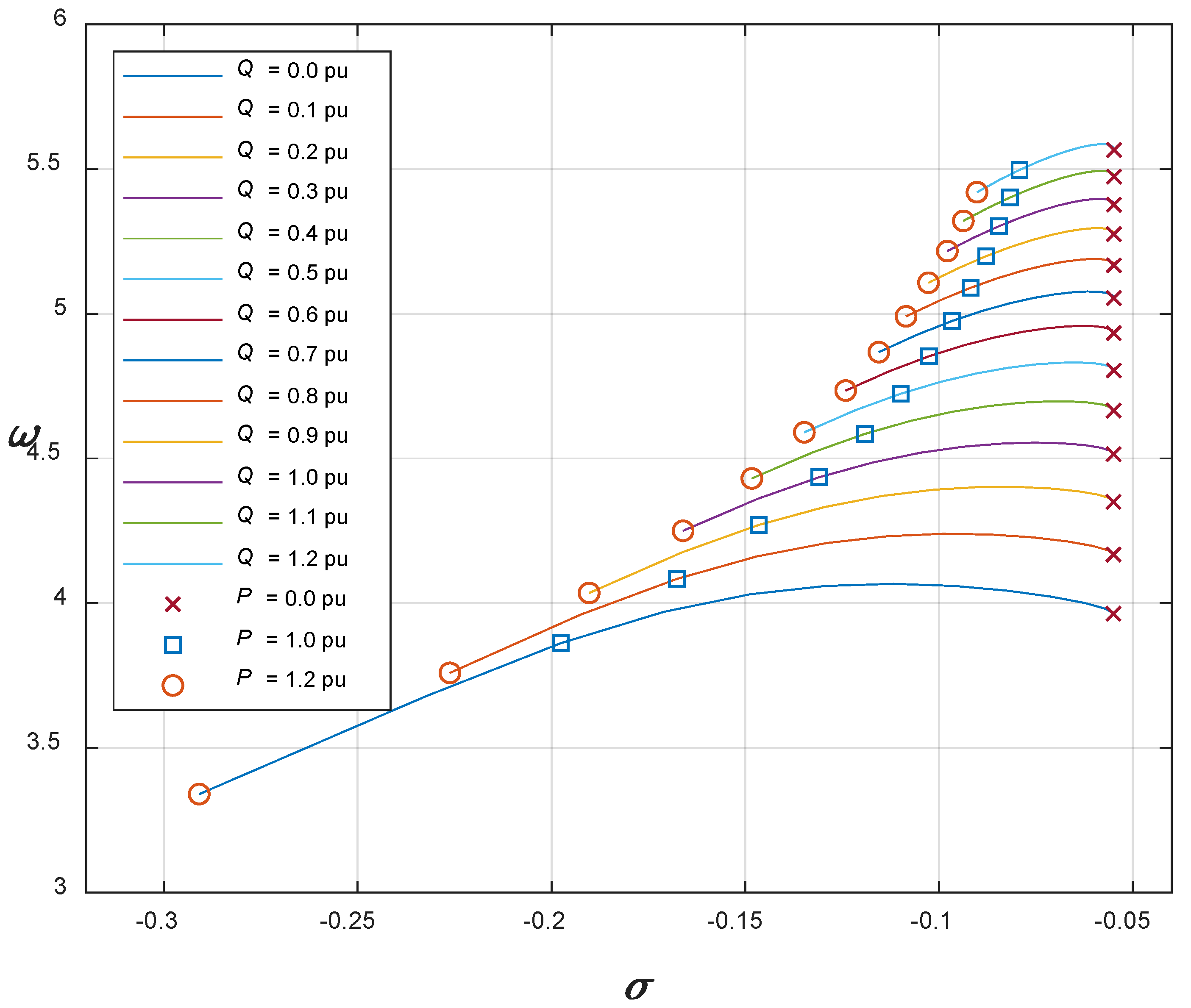
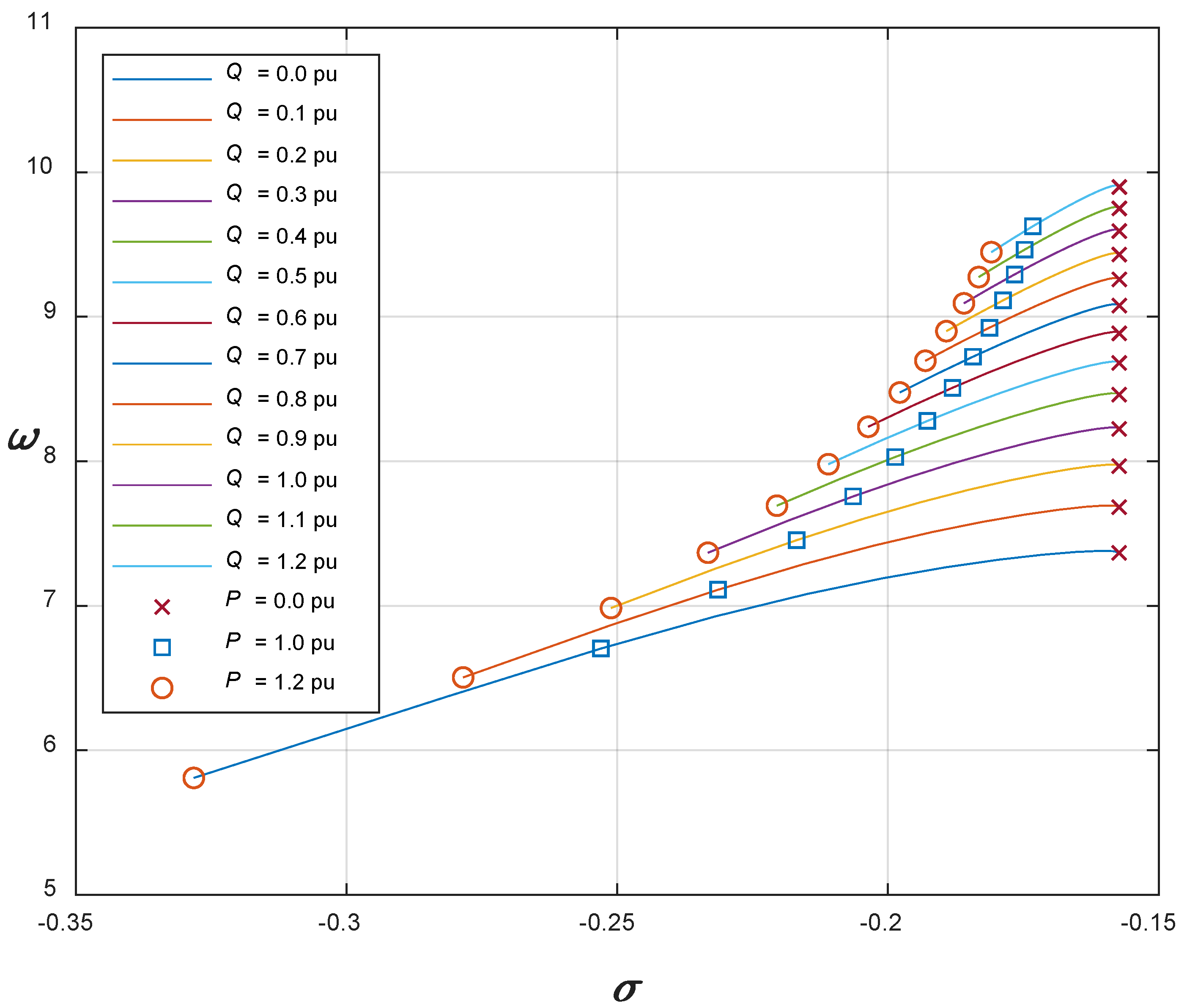
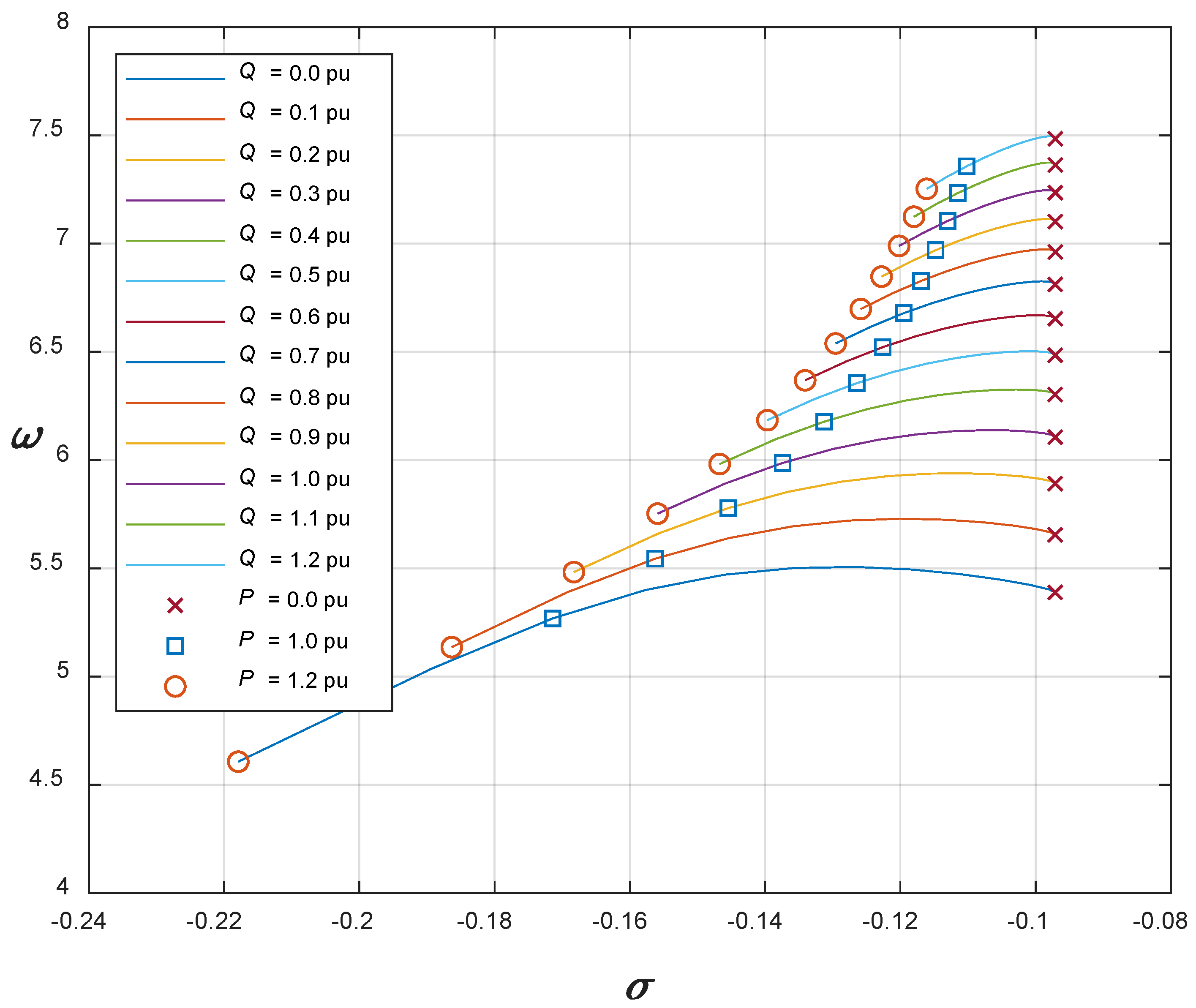
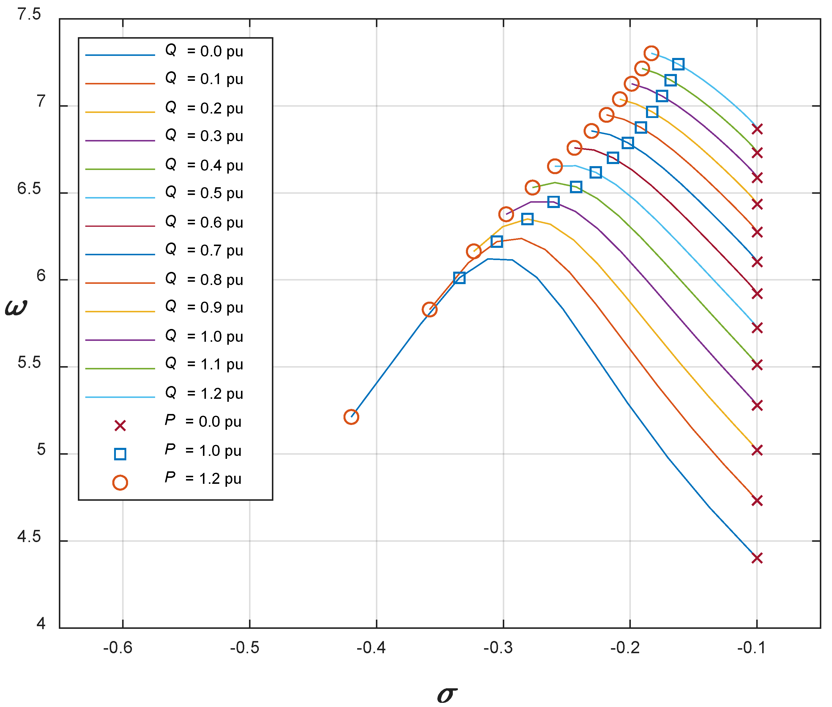
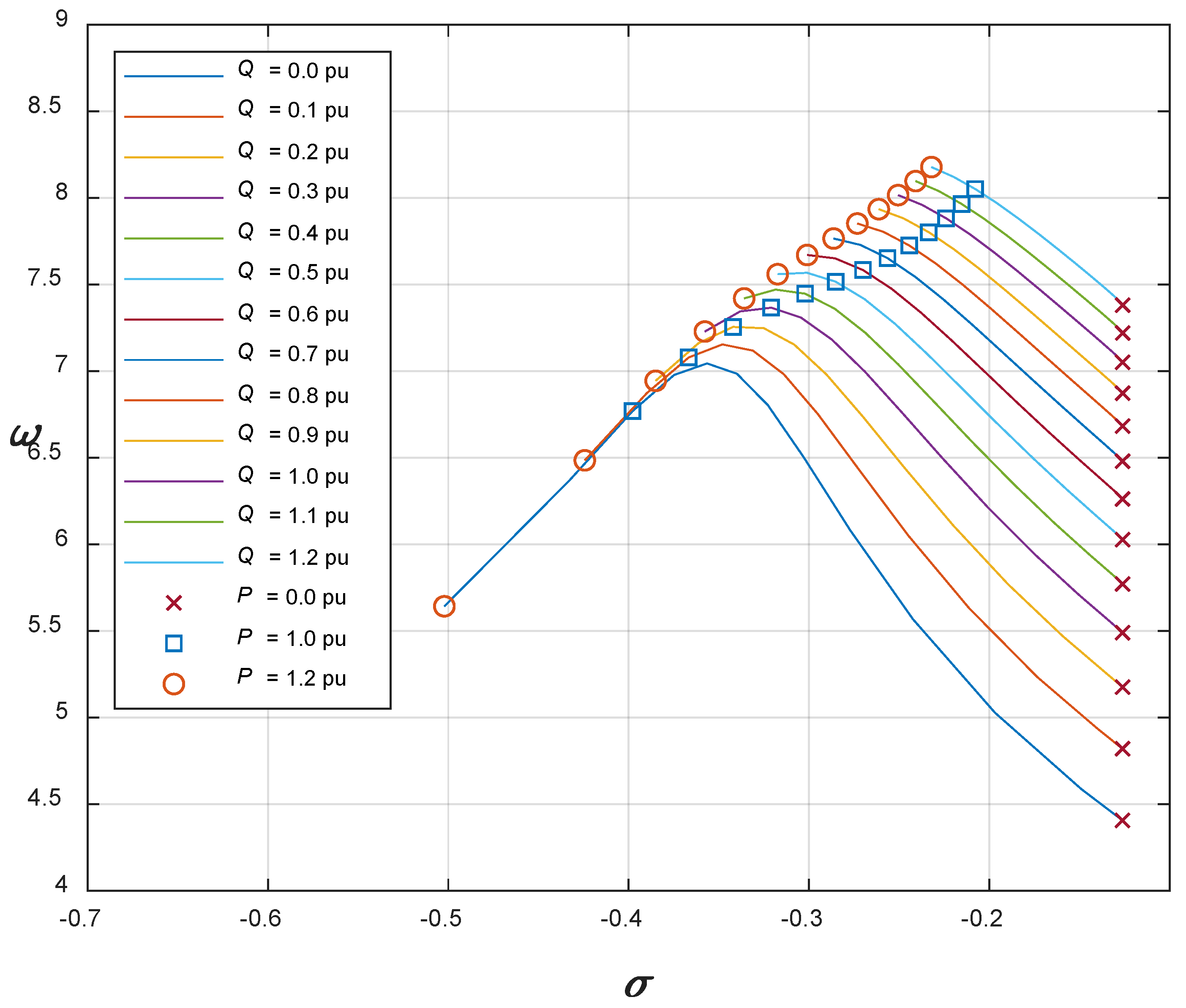
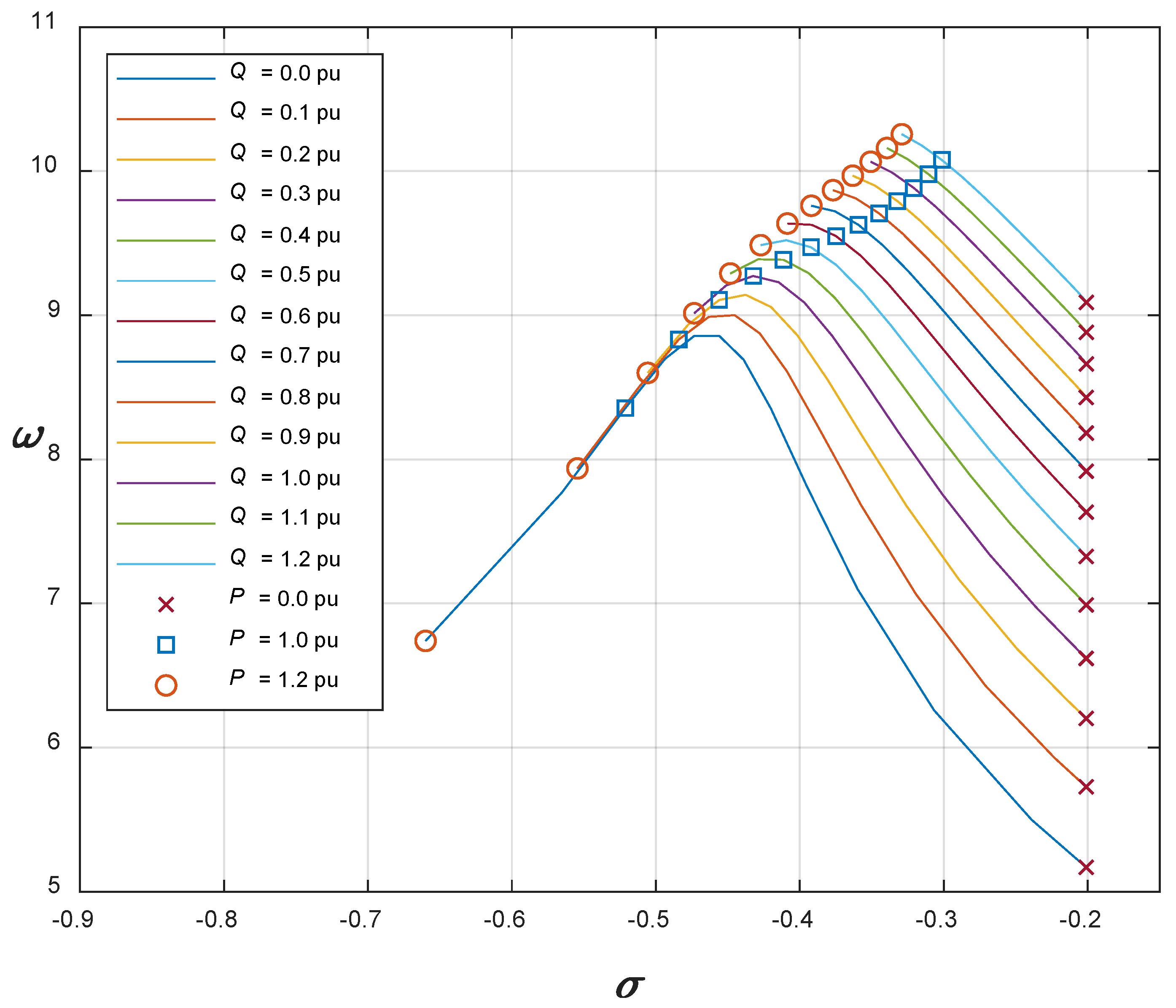
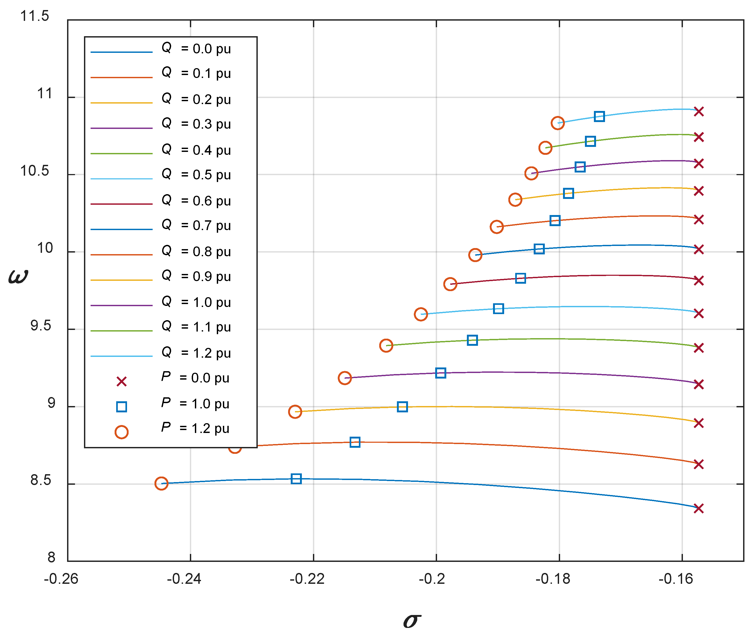
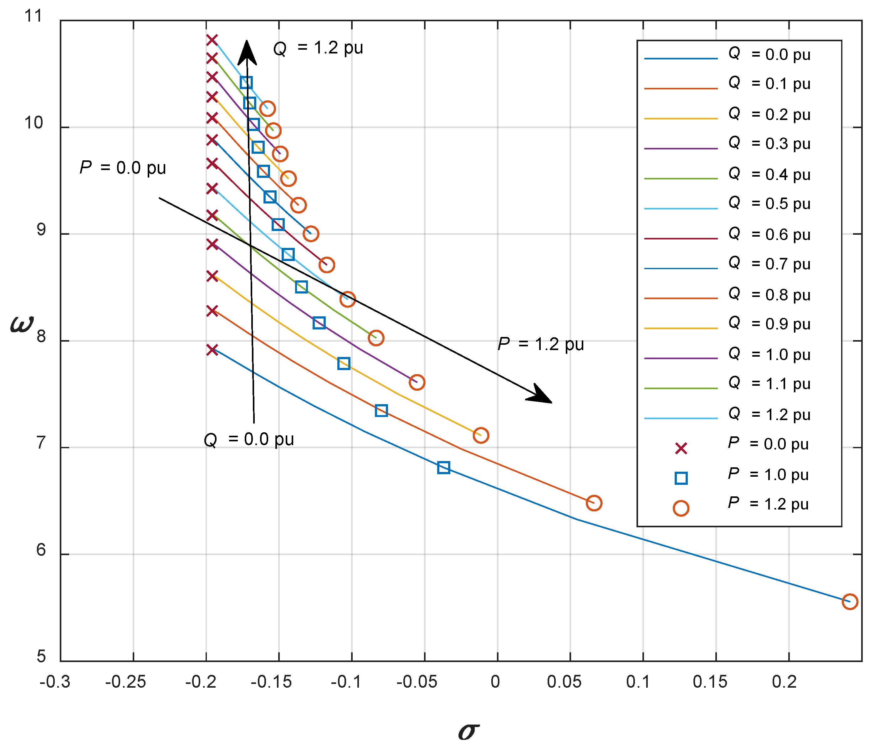
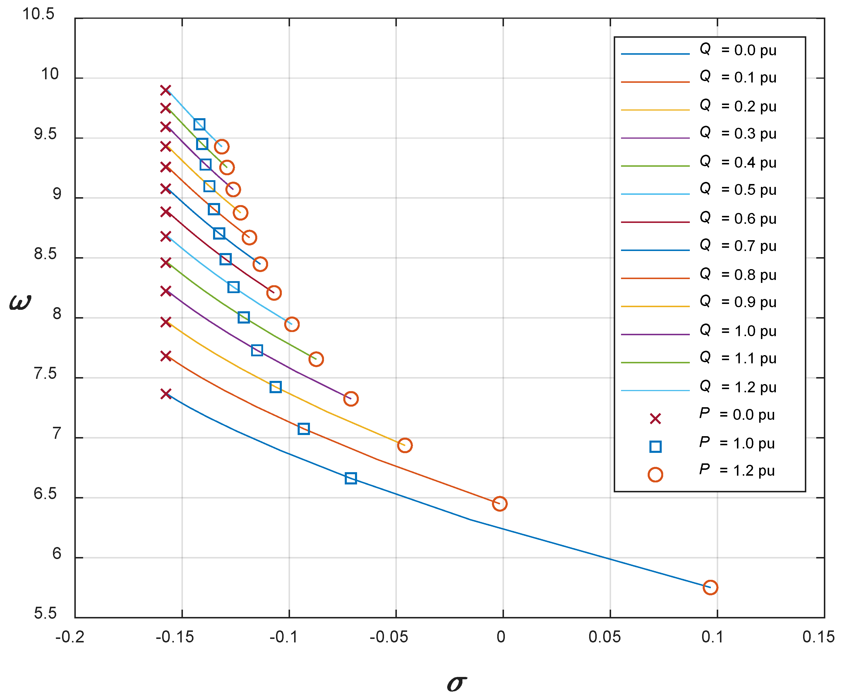
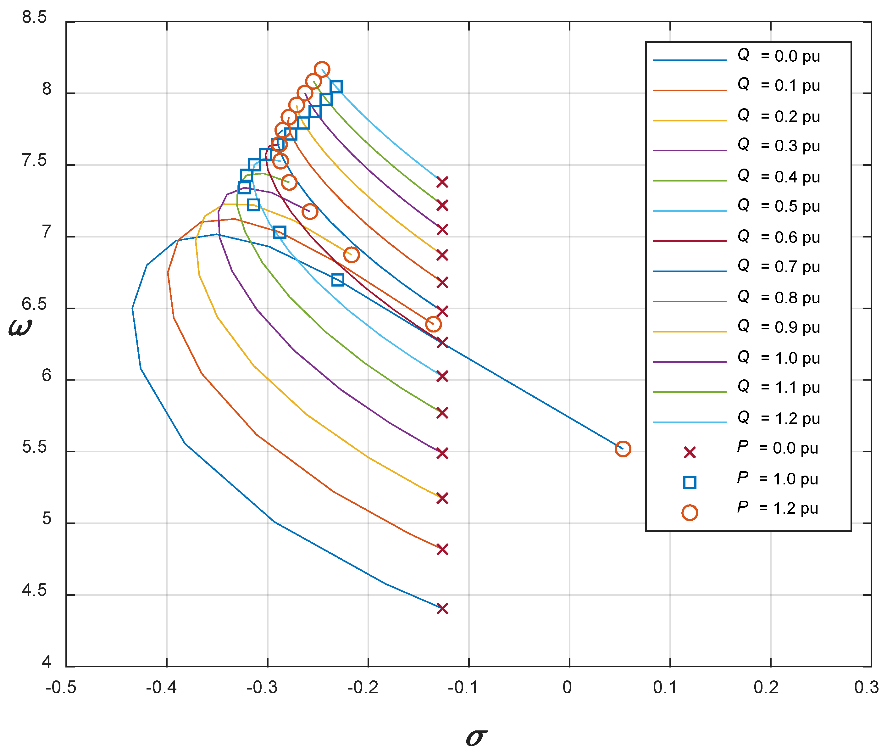
The influence of the operating point on the synchronous generator’s local oscillations can be evaluated by eigenvalue loci analysis. Hydro-type synchronous generators of nominal powers in the range of 9 MVA to 615 MVA, with data in Appendix A, Table A1, Table A2,

Table A3. Manufacturer’s data: hydro-type synchronous generator S_n = 158 MVA.

Sn = 158 [MVA]	Un = 13.8 [kV]	cos φn = 0.9	H = 3.18 [pu]
Ld = 0.920 [pu]	Lq = 0.510 [pu]	Ld′ = 0.300 [pu]	Ld″ = 0.220 [pu]
Rs = 0.045 [pu]	RF = 0.206 [pu]	Td0′= 4.2 [s]	D = 2 [pu]

and

Table A4. Manufacturer’s data: hydro-type synchronous generator S_n = 615 MVA.

Sn = 615 [MVA]	Un = 15 [kV]	cos φn = 0.975	H = 5.15 [pu]
Ld = 0.900 [pu]	Lq = 0.650 [pu]	Ld′ = 0.300 [pu]	Ld″ = 0.230 [pu]
Rs = 0.045 [pu]	RF = 0.181[pu]	Td0′ = 7.4 [s]	D = 2 [pu]

, were analyzed first. Dominant conjugate complex eigenvalues of the system matrix of the H–P model (1) were calculated for different operating points. Figure 1, Figure 2, Figure 3 and Figure 4 show the local mode eigenvalue loci as a function of operating points for synchronous generators with nominal powers 9 MVA, 12 MVA, 158 MVA, and 615 MVA. Active power ranged from 0.0 pu to 1.2 pu at constant reactive power. The calculations were performed at reactive power values from 0.0 pu to 1.2 pu in steps of 0.1 pu. The individual curves correspond to a constant reactive power. Local mode eigenvalues at nominal power P = 1 pu are marked in the figures with squares.

Eigenvalue analysis was carried out for 54 hydro-generators (the figures represent only four of them). It was an interesting discovery that all eigenvalue loci had similar courses. From the obtained loci, four basic conclusions were obtained:

-

An increase in active power results in an increase in local mode damping (decrease in eigenvalues’ real part σ).

-

An increase in reactive power results in an increase in local mode damped frequency (increase in eigenvalues’ imaginary part ω),

-

Stability high-problematic situations could be operating points with high values of reactive power and low values of active power, which have minimal damping.

-

Stability low-problematic situations could be operating points with low values of reactive power and high values of active power, which have maximal damping.

3.2.2. Turbo-Type Synchronous Generators

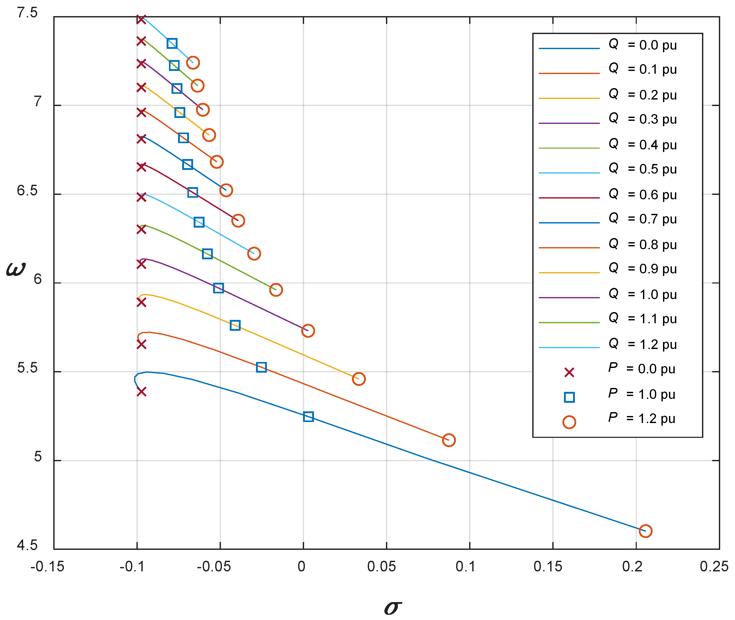
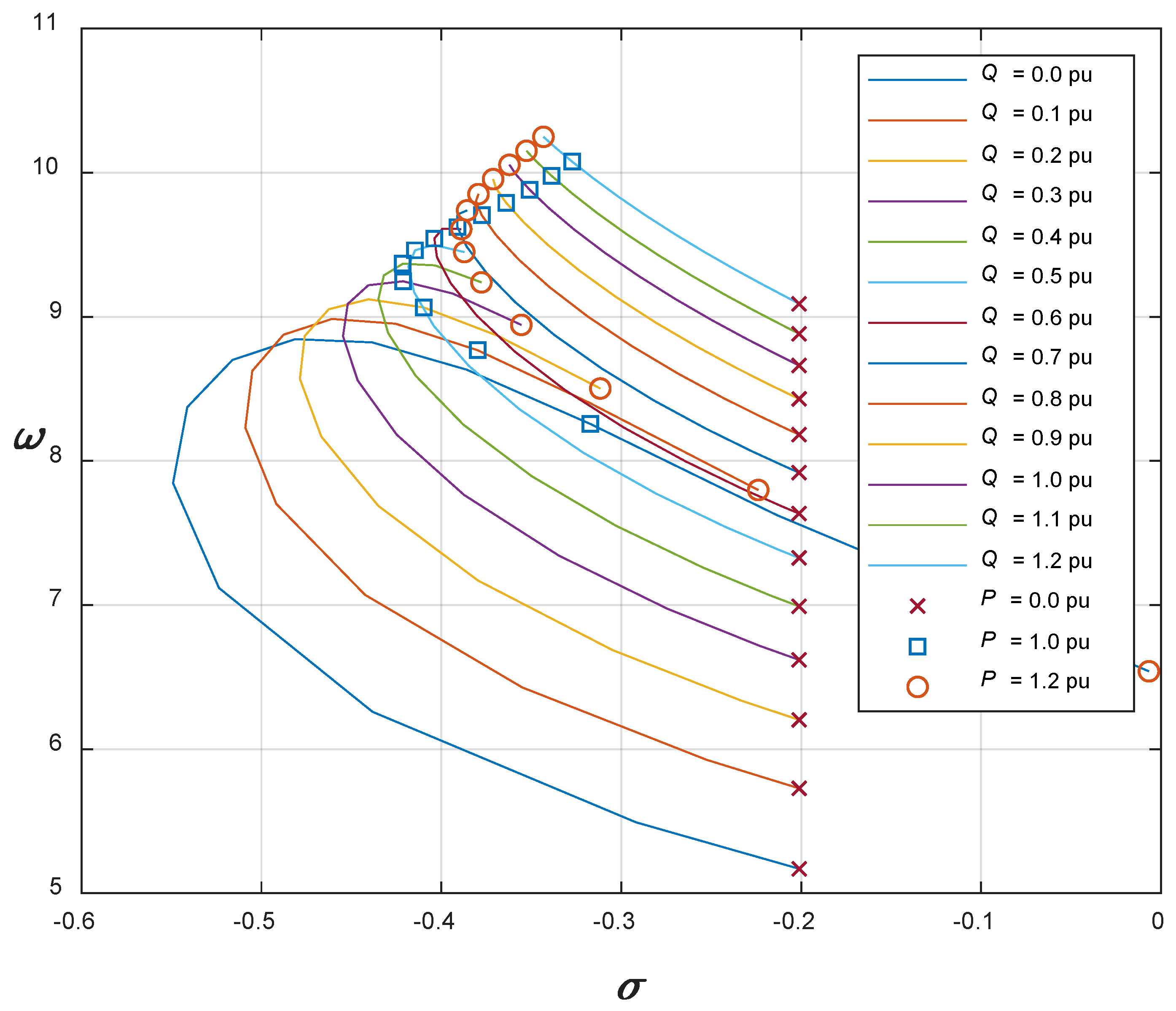
Turbo-type synchronous generators of nominal powers were analyzed in the range of 25 MVA to 911 MVA, with data in Appendix A,

Table A5. Manufacturer’s data: turbo-type synchronous generator S_n = 25 MVA.

Sn = 25 [MVA]	Un = 13.8[kV]	cos φn = 0.8	H = 5.02 [pu]
Ld = 1.250 [pu]	Lq = 1.220 [pu]	Ld′ = 0.232 [pu]	Ld″ = 0.120 [pu]
Rs = 0.008 [pu]	RF = 0.375[pu]	Td0′= 4.75 [s]	D = 2 [pu]

,

Table A6. Manufacturer’s data: turbo-type synchronous generator S_n = 160 MVA.

Sn = 160 [MVA]	Un = 15 [kV]	cos φn = 0.85	H = 3.96 [pu]
Ld = 1.700 [pu]	Lq = 1.640 [pu]	Ld′ = 0.245 [pu]	Ld″ = 0.185 [pu]
Rs = 0.016 [pu]	RF = 0.370 pu	Td0′= 5.9 [s]	D = 2 [pu]

and

Table A7. Manufacturer’s data: turbo-type synchronous generator S_n = 911 MVA.

Sn = 911 [MVA]	Un = 26 kV	cos φn = 0.9	H = 2.49 [pu]
Ld = 2.04 [pu]	Lq = 1.96 [pu]	Ld′ = 0.266 [pu]	Ld″ = 0.193 [pu]
Rs = 0.001 [pu]	RF = 0.121[pu]	Td0′= 6.0 [s]	D = 2 [pu]

. The same eigenvalue analysis was performed as for hydro-generators. Figure 5, Figure 6 and Figure 7 show the eigenvalue loci as a function of operating point for synchronous generators with nominal powers 25 MVA, 160 MVA, and 911 MVA.

Eigenvalue analysis was carried out for 48 turbo-generators. For all generators, similar eigenvalue loci were obtained, as shown in Figure 5, Figure 6 and Figure 7. The eigenvalue loci of turbo-generators differ from the loci of hydro-generators in that the loci of the constant reactive power of turbo-generators are not so straightforward, especially for the curves of low reactive power, whose convexity is evident in the vicinity of the nominal values of the active power. The primary conclusions that the increase in active power decreases the real part σ, and that the increase in reactive power increases the imaginary part ω, still apply. Additionally, the oscillations are better damped at operating points with high values of active power and low values of reactive power. The damping is smaller at high values of reactive power and low values of active power.

3.3. Influences of the Transmission Line between Synchronous Generator and Infinite Bus and the Size of Synchronous Generators on Local Mode Eigenvalues

Local mode eigenvalues depend on the synchronous generators’ parameters and the parameters of the transmission line between the synchronous generator and infinite bus. In the previous section, simulations were carried out with parameters of a real transmission line. It is to be expected that lower transmission line impedance results in higher frequency. For detailed insight, the eigenvalue analyses were performed for cases with different values of transmission line impedance.

Figure 8 shows the eigenvalue loci of a 158-MVA hydro-type synchronous generator where transmission line impedance was reduced to 50% of its nominal value. Figure 8 could be compared directly to Figure 3. From this analysis, it is visible that changes in transmission line impedance influence the local mode eigenvalues so that a decrease in impedance results in increased oscillation frequency. Because the transmission line parameters usually stay unchanged during the operation, and because this influence is relatively small, a detailed analysis of the correlation between transmission line parameters and local mode eigenvalues is not presented.

Interestingly, it is not possible to conclude how the size of generators correlates with the frequency and damping of oscillations. From Figure 1 and Figure 2, it is evident that generators of similar size (nominal powers 9 MVA and 12 MVA) have (similar courses, but) completely different values of oscillations’ frequency and damping. There are also cases where generators with significantly different nominal powers have very similar eigenvalues loci. The conclusion is that more than the size affects the synchronous generator’s construction in terms of its local mode eigenvalues.

3.4. Local Mode Boundaries’ Assessment

However, it is beneficial to estimate what the boundary values of damped frequencies ω and time constants of amplitude decay σ of local oscillations are for synchronous generators of different types and different nominal powers. The boundary assessment aimed to estimate the frequencies and dampings of the local oscillations of the currently operating synchronous generators for all possible loadings. The obtained results allow us to predict local oscillations’ frequencies and dampings and will be useful in PSS planning. The eigenvalues were calculated for more than one hundred real synchronous generators connected to the infinite bus (all synchronous generators in the Slovenian power system were analyzed, plus some synchronous generators for which data were attainable from the literature). It was assumed that generator loads range from 0 to 120% in active and reactive power (generators were over-excited, and they deliver reactive power at lagging power factor). The boundaries were estimated based on systematic calculations. The obtained values are presented in

Table 3. The boundaries of real and imaginary parts of local mode eigenvalues of hydro and turbo synchronous generators of different nominal powers in an operating range from P = 0.0 pu to P = 1.2 pu and from Q = 0.0 pu to Q = 1.2 pu.

	Σmin	σmax	ωmin (s−1)	ωmax (s−1)
hydro-generators	−0.4558	−0.0399	2.8554	10.8259
turbo-generators	−0.8871	−0.0807	3.6418	10.5455

.

In cases where the generator loads range from 0 to 100% in active and reactive power (generators were over-excited, and they deliver reactive power at lagging power factor), the calculated boundaries are presented in

Table 4. The boundaries of real and imaginary parts of local mode eigenvalues of hydro and turbo synchronous generators of different nominal powers in an operating range from P = 0.0 pu to P = 1.0 pu and from Q = 0.0 pu to Q = 1.0 pu.

	σmin	σmax	ωmin (s−1)	ωmax (s−1)
hydro-generators	−0.3193	−0.0399	3.3636	9.1832
turbo-generators	−0.6361	−0.0807	3.6418	9.4520

.

Of course, the results are primarily valid for synchronous generators in the Slovenian power system. Still, due to similar generators in European power plants, the results are advantageous for engineers and researchers working in the European Network of Transmission System Operators.

4. Local Mode Analysis of Synchronous Generators with AVR

4.1. Synchronous Generators’ Voltage Control Systems

Synchronous generators operating in a power system require an extensive control system for coordinated operation. There are two fundamental synchronous generator control systems: a primary speed control system (i.e., frequency restoration control system) and a voltage control system. The main difference between these two control systems is in the response speed of the final control element. Turbines that generate the mechanical torque needed in primary speed control systems are very slow-acting, so this control system does not affect synchronous generators’ electromechanical oscillations significantly. On the other hand, exciters in modern power plants are almost always static semiconductor devices, which are considerably faster and influence electromechanical oscillations greatly. Voltage control systems can decrease the damping of the local oscillations significantly.

New voltage control systems for synchronous generators are often realized with a cascade control system, where the outer control loop regulates the voltage (or reactive power), and the inner loop maintains the static U/Q characteristic. Both control loops could be implemented with proportional–integral (PI) controllers. However, many synchronous generators are still equipped with a simple voltage control system based on a proportional (P)-type voltage controller and static exciter.

This control system performs voltage regulation and provides the static U/Q characteristic. Such a voltage control concept is the most transparent for analysis and also the most commonly used in similar studies [11,12,13]. Therefore, we also limited this study to the analysis of the influence of this type of voltage control system on the local mode eigenvalues.

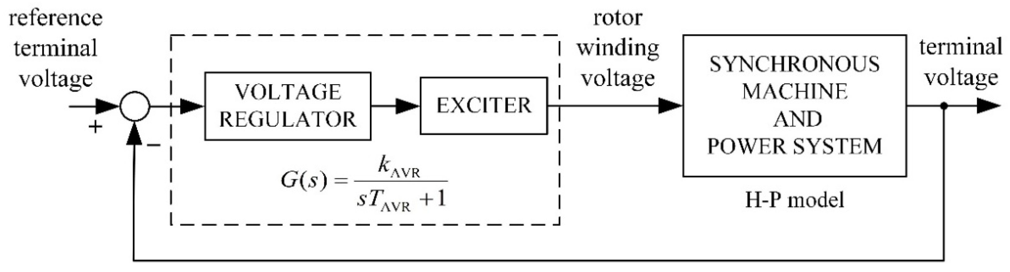
A voltage control system with a P-controller and static exciter has a significant impact on local oscillations. The controller in this system is usually called an automatic voltage regulator (AVR). The block diagram of the AVR system is shown in Figure 9. This simple control system essentially changes the synchronous generator dynamics.

The simplest mathematical model of the regulator in series with the exciter is a first-order lag, described with the transfer function:

$$G(s)=\frac{E_{\mathrm{FD}\mathsf{\Delta }}(s)}{V_{\mathrm{t}\mathsf{\Delta },\mathrm{ref}}(s)-V_{\mathrm{t}\mathsf{\Delta }}(s)}=\frac{k_{\mathrm{AVR}}}{s{T}_{\mathrm{AVR}}+1}$$

(5)

where V_tΔ,ref(s) represents the reference terminal (stator) voltage, V_tΔ(s) represents the actual terminal voltage, and E_fdΔ(s) represents the output from the exciter, i.e., rotor winding voltage. All symbols denote Laplace transforms of time deviation signals where s is a complex frequency variable and _Δ denotes deviations. The symbol k_AVR represents the product of the voltage controller and exciter gains, and T_AVR represents the exciter time constant. The time constant T_AVR depends on the available exciter. For a static exciter, T_AVR is very short. It is mainly in the range of 2–10 ms.

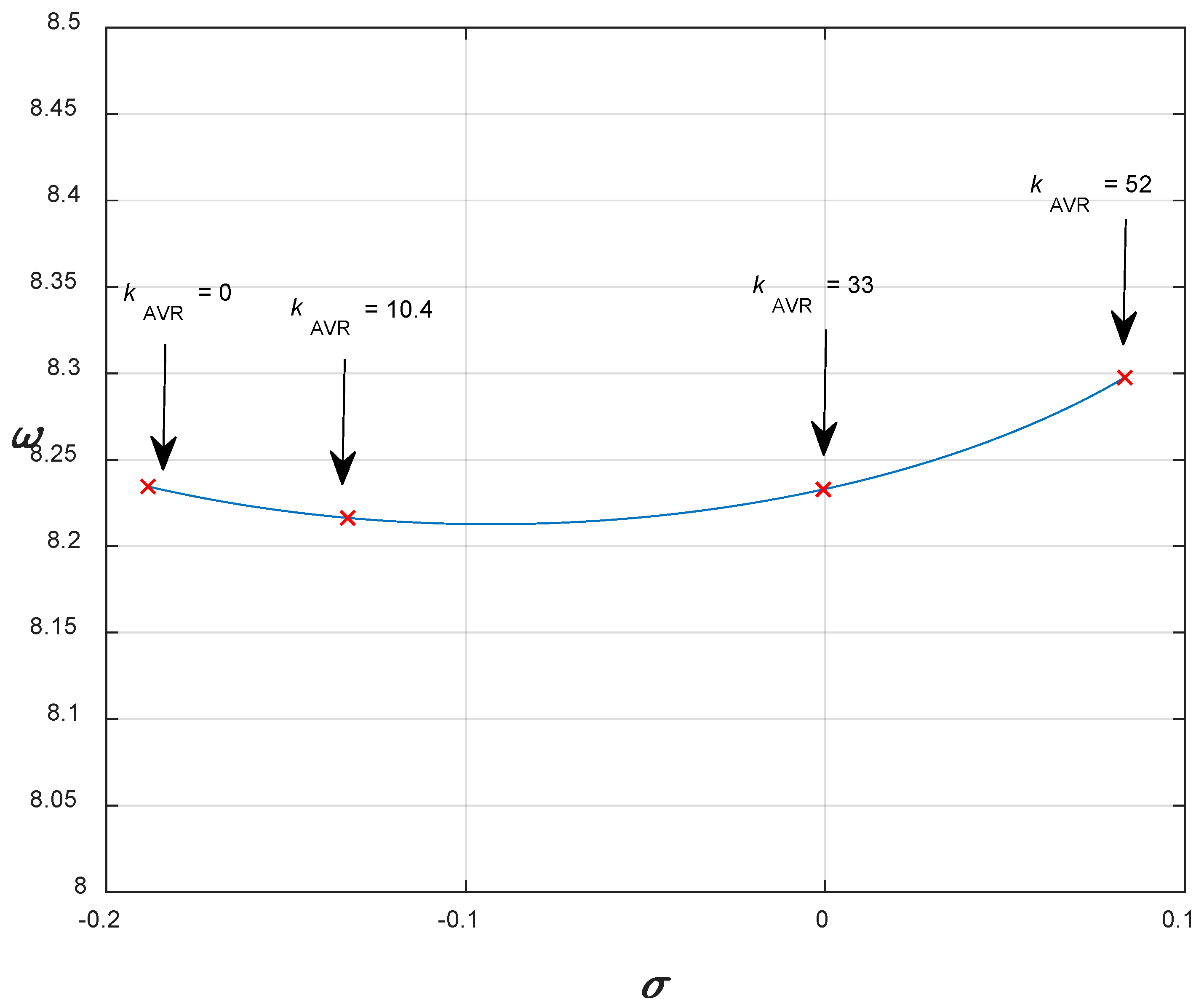
There are many publications that have studied the tuning of the gain k_AVR. The rule for setting k_AVR was described for the first time in [21]. In [21], it was derived that for the well-damped performance of the voltage control loop, it is desirable to maintain a crossover frequency lower than 1/(2 T_AVR), which would mean that the gain k_AVR “should be approximately less than T’_d0/(2T_AVR)”. Later, in [22], it was shown that gain k_AVR has a significant impact on the local mode eigenvalue and that the k_AVR values which are close to the estimated maximal value T’_d0/(2 T_AVR) cause instability. Therefore, in this work, the impact of the gain k_AVR on the local mode eigenvalue was considered first.

The H–P model (Equations (1) and (2)), extended with the mathematical model of the AVR system (Equation (5)), is presented with Equations (6) and (7).

$$\left[\begin{array}{c}{\dot{\delta }}_{\mathsf{\Delta }}(t)\\ {\dot{\omega }}_{\mathsf{\Delta }}(t)\\ {{\dot{E}}^{\prime }}_{\mathrm{q}\mathsf{\Delta }}(t)\\ {\dot{E}}_{\mathrm{fd}\mathsf{\Delta }}(t)\end{array}\right]=\left[\begin{array}{cccc}0& {\omega }_{\mathrm{s}}& 0& 0\\ -\frac{K_1}{2H}& -\frac{D}{2H}& -\frac{K_2}{2H}& 0\\ -\frac{K_4}{{T^{\prime }}_{\mathrm{d}0}}& 0& -\frac{1}{{T^{\prime }}_{\mathrm{d}0}{K}_3}& \frac{1}{{T^{\prime }}_{\mathrm{d}0}}\\ -\frac{k_{\mathrm{AVR}}{K}_5}{T_{\mathrm{AVR}}}& 0& -\frac{k_{\mathrm{AVR}}{K}_6}{T_{\mathrm{AVR}}}& -\frac{1}{T_{\mathrm{AVR}}}\end{array}\right]\left[\begin{array}{c}{\delta }_{\mathsf{\Delta }}(t)\\ {\omega }_{\mathsf{\Delta }}(t)\\ {E^{\prime }}_{\mathrm{q}\mathsf{\Delta }}(t)\\ E_{\mathrm{fd}\mathsf{\Delta }}(t)\end{array}\right]+\left[\begin{array}{cc}0& 0\\ \frac{1}{2H}& 0\\ 0& 0\\ 0& \frac{k_{\mathrm{AVR}}}{T_{\mathrm{AVR}}}\end{array}\right]\left[\begin{array}{c}{T}_{\mathrm{m}\mathsf{\Delta }}(t)\\ V_{\mathrm{t},\mathrm{ref}\mathsf{\Delta }}(t)\end{array}\right]$$

(6)

$$\left[\begin{array}{c}{T}_{\mathrm{e}\mathsf{\Delta }}(t)\\ V_{\mathrm{t}\mathsf{\Delta }}(t)\end{array}\right]=\left[\begin{array}{l}\begin{array}{ccc}{K}_1& 0& K_2\end{array}\\ \begin{array}{ccc}{K}_5& 0& K_6\end{array}\end{array}\right]\left[\begin{array}{cccc}{K}_1& 0& K_2& 0\\ K_5& 0& K_6& 0\end{array}\right]\left[\begin{array}{c}{\delta }_{\mathsf{\Delta }}(t)\\ {\omega }_{\mathsf{\Delta }}(t)\\ {E^{\prime }}_{\mathrm{q}\mathsf{\Delta }}(t)\\ E_{\mathrm{fd}\mathsf{\Delta }}(t)\end{array}\right]+\left[\begin{array}{cc}0& 0\\ 0& 0\end{array}\right]\left[\begin{array}{c}{T}_{\mathrm{m}\mathsf{\Delta }}(t)\\ V_{\mathrm{t},\mathrm{ref}\mathsf{\Delta }}(t)\end{array}\right]$$

(7)

4.2. Influence of AVR Gain k_AVR on Local Mode Eigenvalues of Synchronous Generators with AVR System

The AVR gain k_AVR has a significant influence on the synchronous generator dynamics. The eigenvalues of the extended H–P model (Equations (6) and (7)) must be calculated to analyze the local oscillations of the synchronous generator with the AVR system. The obtained characteristic equation is presented with (Equation (8)).

$$\begin{array}{l}2K_{3}H{T^{\prime }}_{d0}{T}_{AVR}{\lambda }^4+\\ \left(K_{3}D{T^{\prime }}_{d0}{T}_{AVR}+2H{T}_{AVR}+2H{K}_3{T^{\prime }}_{d0}\right)\hspace{0.17em}{\lambda }^3+\\ \left(K_1{K}_3{T^{\prime }}_{d0}{T}_{AVR}{\omega }_{\mathrm{s}}+D{T}_{AVR}+K_{3}D{T^{\prime }}_{d0}+2K_3{K}_6{K}_{AVR}H+2H\right)\hspace{0.17em}{\lambda }^2+\\ \left(K_3{K}_6{K}_{AVR}D+K_1{K}_3{T^{\prime }}_{d0}{\omega }_{\mathrm{s}}+D+K_1{T}_{AVR}{\omega }_{\mathrm{s}}-K_2{K}_3{K}_4{T}_{AVR}{\omega }_{\mathrm{s}}\right)\hspace{0.17em}\lambda +\\ \left(K_1{K}_3{K}_6{K}_{AVR}{\omega }_{\mathrm{s}}-K_2{K}_3{K}_5{K}_{AVR}{\omega }_{\mathrm{s}}+K_1{\omega }_{\mathrm{s}}-K_2{K}_3{K}_4{\omega }_{\mathrm{s}}\right)=0\end{array}$$

(8)

The impact of the gain k_AVR on the local mode eigenvalue of the hydro-type synchronous generator of nominal power 158 MVA is shown in Figure 10. From the recommendation in [21], it is calculated that the gain value k_AVR for this synchronous generator and the belonging exciter must be lower than 52 (T’_d0 = 5.2 s, T_AVR = 0.05 s). From the numerical analysis, it is clearly evident that such gain value k_AVR causes instability and that the gain value that assures stable operation must be significantly lower than the recommended gain k_AVR [21]. Similar correlations between gain k_AVR and local mode eigenvalue were obtained for all synchronous generators for all operating points.

4.3. Influence of Operating Point of Synchronous Generators with the AVR System on Local Mode Eigenvalues

4.3.1. Hydro-Type Synchronous Generators

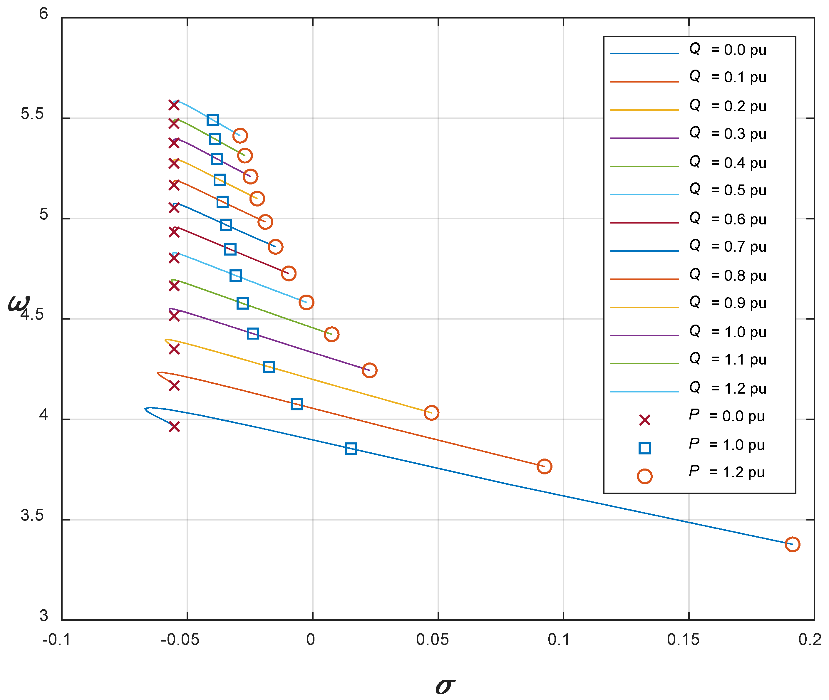
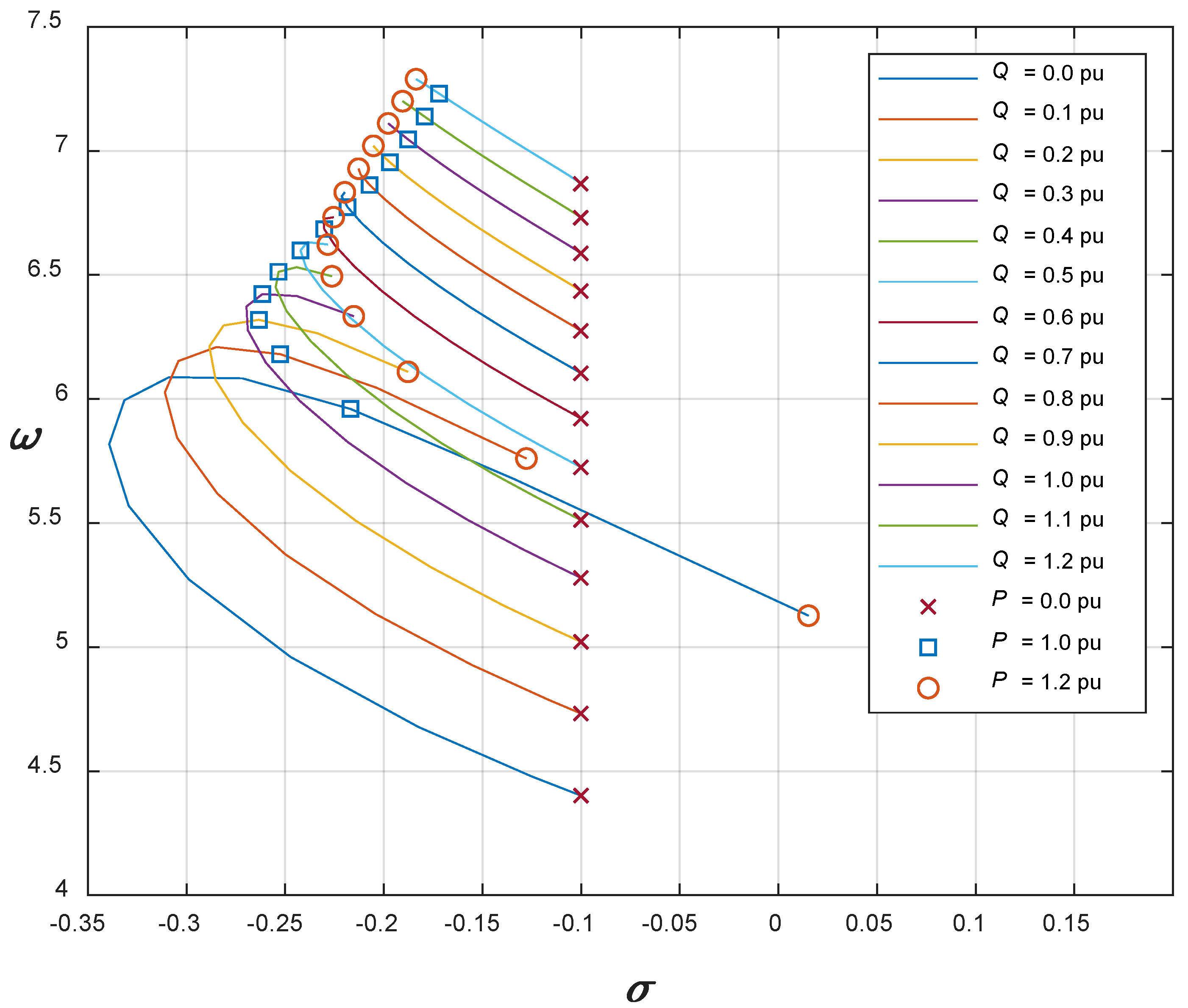
The same hydro-type synchronous generators were analyzed as in Section 3.2.1. All synchronous generators were equipped with the AVR system with the AVR and exciter, modeled with Equation (5). Exciters with the time constant T_AVR = 0.05 s were used in all cases. The gains k_AVR were calculated according to the theoretically, numerically, and empirically confirmed equation k_AVR = T’_d0/(10·T_AVR). The coefficients of the H–P models for operating points in the entire operating range were calculated for all synchronous generators. Active power ranged from 0.0 pu to 1.2 pu, and reactive power ranged from 0.0 pu to 1.2 pu at lagging power factor. The local mode eigenvalues were calculated from (8). Figure 11, Figure 12, Figure 13 and Figure 14 show the eigenvalue loci as a function of the operating point for synchronous generators with nominal powers 9 MVA, 12 MVA, 158 MVA, and 615 MVA. The individual curves correspond to the constant reactive power (values from 0.0 pu to 1.2 pu in steps of 0.1 pu). Active power ranged from 0.0 pu to 1.2 pu.

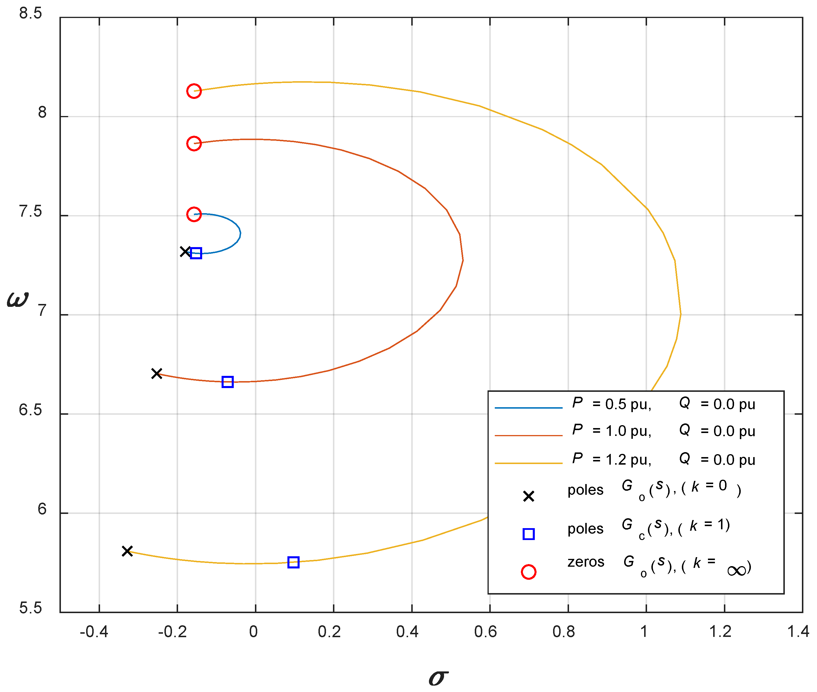
Eigenvalue analysis was carried out for all studied hydro-generators. Even in the case of hydro-generators with AVR systems, the curves showing the dependence of local mode eigenvalues on the operating point have similar forms for hydro-generators of different powers. While in hydro-generators without AVR systems, the increase in active power in all cases led to a decrease in the real part of the eigenvalue of the local mode, and thus to an increase in damping of oscillations, in hydro-generators with AVR systems, an increase in active power leads to an increase in the local mode eigenvalue’s real part, and thus to a reduction in damping or even instability. The root locus diagram for open-loop transfer function G_o(s) clearly shows the influence of the AVR on the stability of a closed-loop transfer function G_c(s):

$$G_{\mathrm{o}}(s)=\frac{V_{\mathrm{t}\mathsf{\Delta }}(s)}{E(s)}=\frac{b_{\mathrm{o}2}{s}^2+b_{\mathrm{o}1}s+b_{\mathrm{o}0}}{a_{\mathrm{o}4}{s}^4+a_{\mathrm{o}3}{s}^3+a_{\mathrm{o}2}{s}^2+a_{\mathrm{o}1}s+a_{\mathrm{o}0}}$$

(9)

$$G_{\mathrm{c}}(s)=\frac{V_{\mathrm{t}\mathsf{\Delta }}(s)}{V_{\mathrm{t}\mathsf{\Delta },\mathrm{ref}}(s)}=\frac{b_{\mathrm{c}2}{s}^2+b_{\mathrm{c}1}s+b_{\mathrm{c}0}}{a_{\mathrm{c}4}{s}^4+a_{\mathrm{c}3}{s}^3+a_{\mathrm{c}2}{s}^2+a_{\mathrm{c}1}s+a_{\mathrm{c}0}}$$

(10)

where E(s) represents the input in the AVR, V_tΔ(s) is the terminal stator voltage deviation, V_tΔ,ref(s) is the reference terminal voltage deviation, and a_i and b_i are transfer functions’ coefficients.

Figure 15 shows the root locus diagrams of local mode eigenvalue for a hydro synchronous generator with nominal power 158 MVA at three operating points: (i) P = 0.0 pu, Q = 0.0 pu; (ii) P = 0.0 pu, Q = 0.0 pu; and (iii) P = 0.0 pu, Q = 0.0 pu. All curves start in the local mode poles of G_o(s) and end in the corresponding zeros of G_o(s). With “square ” are denoted closed-loop poles at gain k_AVR = 10.4.

The findings obtained from the numerical analysis of all synchronous generators can be summarized in four conclusions:

-

An increase in active power results in a decrease in local mode damping and can lead to instability.

-

An increase in reactive power results in an increase in local mode frequency,

-

The minimal damping has operating points with low values of reactive power and high values of active power.

-

The maximal damping has operating points with high values of reactive power and low values of active power.

4.3.2. Turbo-Type Synchronous Generators

The analysis was also performed on the dependence of local mode eigenvalues on the operating point for turbo-type synchronous generators with rated powers of 25 MVA to 911 MVA. Figure 16, Figure 17 and Figure 18 show the eigenvalue loci for synchronous generators with nominal powers 25 MVA, 160 MVA, and 911 MVA.

Again, the eigenvalue curves had a similar shape for all turbo-type synchronous generators of different powers equipped with an AVR system. It can be seen that the increase in active power can have a negative effect on damping or causes instability only at very small values of reactive power and at very large values of active power. In the remaining (larger) part of the operating range, changing the produced active and reactive power has a similar effect on local mode eigenvalues as that of turbo-type synchronous generators without AVR.

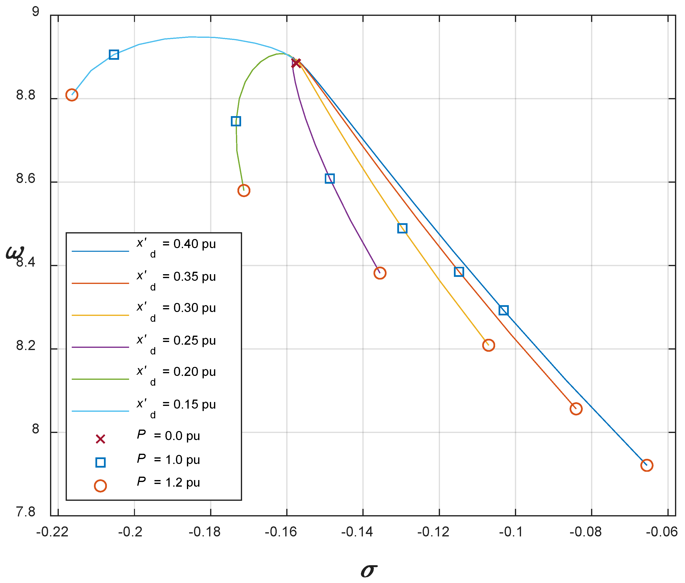
It is interesting to note that the increase in active power for hydro-type synchronous generators with an AVR system reduces damping, as seen in Figure 11, Figure 12, Figure 13 and Figure 14, while the increase in active power in turbo-type generators in most areas of the operating range reduces damping, as seen in Figure 16, Figure 17 and Figure 18. We were interested to find out which construction parameter was crucial for such different behavior of both types of synchronous generators. We analyzed all the parameters of generator models of different rated powers. The analysis showed that a key impact on the correlation between the real part of eigenvalues and the generated active power represents the direct-axis transient reactance x_d’. Turbo-type synchronous generators generally have lower x_d’ values than hydro-types, which is described in the references and was also confirmed by our data. According to [4], the turbo-type generators have direct-axis transient reactances x_d’ in the range 0.15–0.4, and hydro-type in the range 0.2–0.5. According to [23], the turbo-type generators have reactances in the range 0.23–0.35, and hydro-type in the range 0.25–0.45. From the study, it was observed that different relations between d- and q-axis synchronous reactances for hydro- and turbo-type generators do not cause the aforementioned different influence of active power on eigenvalues’ real parts.

Figure 19 shows six curves of local mode eigenvalues of a hydro-type synchronous generator with nominal power 158 MVA with an AVR system at constant reactive power value Q = 0.6 pu. Each curve represents the eigenvalues at a different simulated value of the direct-axis transient reactance x_d’. The real value of d-axis transient reactance is x_d’ = 0.30; the curves show the eigenvalue loci at x_d’ values in the range from 0.15 to 0.40. It is clearly visible that at higher x_d’ values the increase in power results in a decrease in the damping, and at lower values of x_d’, the increase in power increases the damping of local oscillations.

4.4. Local Mode Boundaries Assessment for Synchronous Generators with AVR

We calculated the boundaries of the area in which their local mode eigenvalues also lay in the case when the AVR system was used for all synchronous generators with available data. For the AVR with the excitation system, we used the mathematical model (5); the T_AVR value was determined by the excitation system, and the k_AVR value was chosen according to the condition k_AVR = T’_d0/(10·T_AVR). The parameters of synchronous generators, excitation systems, and AVR are given in Appendix A for all synchronous generators with the presented results. It was assumed that generator loads range from 0 to 120% (or 0 to 100%) in active and reactive power at lagging power factor. The obtained values are presented in

Table 5. The boundaries of real and imaginary parts of local mode eigenvalues of hydro and turbo synchronous generators with AVR systems of different nominal powers in the range P = 0.0 pu to P = 1.2 pu and from Q = 0.0 pu to Q = 1.2 pu.

	σmin	σmax	ωmin (s−1)	ωmax (s−1)
hydro-generators	−0.2156	0.2804	2.9230	10.8261
turbo-generators	−0.6421	0.3247	3.6418	10.5310

and

Table 6. The boundaries of real and imaginary parts of local mode eigenvalues of hydro and turbo synchronous generators with AVR systems of different nominal powers in the range P = 0.0 pu to P = 1.0 pu and from Q = 0.0 pu to Q = 1.0 pu.

	σmin	σmax	ωmin (s−1)	ωmax (s−1)
hydro-generators	−0.2156	0.0014	3.3636	9.1831
turbo-generators	−0.6421	−0.0809	3.6418	9.4307

.

5. Experimental Analysis of the Laboratory-Size Synchronous Generator

Confirmation of the correctness of numerical calculations and the obtained conclusions was, unfortunately, not possible on synchronous generators in power plants. Therefore, we performed a series of tests to measure the frequencies and damping of local oscillations throughout the entire operating range on a laboratory-size synchronous generator. A salient pole synchronous generator with the nominal power P_n = 12 kW was used for the experiments. The manufacturer’s data are shown in

Table 7. Manufacturer’s data of the tested synchronous generator.

Pn = 12 [kW]	Un = 400 [V]	In = 21.7 [A]	cos φn = 0.8
UFn = 400 [V]	IFn = 21.7 [A]	fn = 50 [Hz]	nn = 1500 [min−1]

.

P_n denotes the rated active power. U_n, I_n, U_Fn, and I_Fn are the rated stator and excitation winding voltages and currents. The f_n and n_n are rated frequency and mechanical speed, respectively.

To determine the synchronous generator’s parameters, the standardized steady-state, transient, and frequency response tests were used [24,25]. The obtained parameters are shown in

Table 8. Synchronous generator’s data obtained with tests.

Ld = 2.11 [pu]	Lq = 1.45 [pu]	Ld′ = 0.25 [pu]	Ld″ = 0.18 [pu]
ld = 0.15 [pu]	lq = 0.15 [pu]	Re = 0.003 [pu]	Le = 0.03 [pu]
Rs = 0.05 [pu]	RF = 0.015 [pu]	H = 0.19 [pu]	D = 1 [pu]
RD = 0.262 [pu]	RQ = 1.08 [pu]	T′d0 = 0.5 [s]	ωs = 2π50 [s−1]

.

For a nominal operating point, the calculated linearization coefficients are given in

Table 9. Linearization parameters of the H–P model for nominal operating point S_n = 15 kVA, cos φ_n = 0.8.

Pn = 0.8 [pu]	K1 = 2.1555	K2 = 2.0815	K3 = 0.1285
Qn = 0.6 [pu]	K4 = 3.5155	K5 = 0.0228	K6 = 0.0998

.

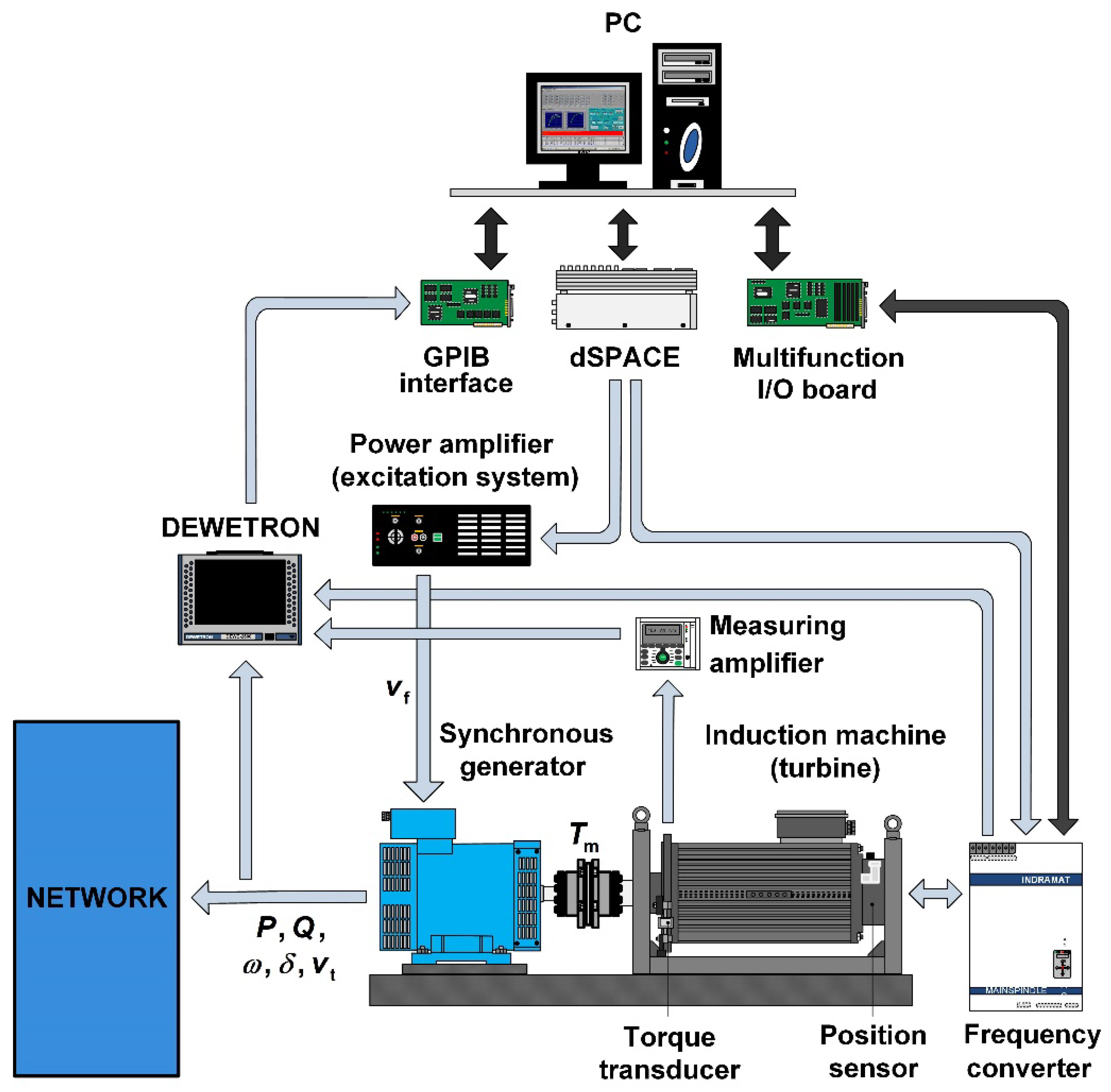
The testing system for the determination of the parameters and for experiments is shown in Figure 20. For the rotor voltage generation, the solid-state power amplifier was used as the excitation system. The induction machine with frequency converter was implemented to produce mechanical torque. The data acquisition system Dewetron was used for recording of time responses. A dSpace R&D controller board was used for control of the power amplifier and frequency converter. Data processing was done using MathWorks/MATLAB.

From the experiments and simulations, it is evident that the 7th-order NLM of a synchronous generator describes well the responses of the laboratory synchronous generator to the changes in both inputs in the entire operating range. Agreement in the first amplitude, the frequency, and the damping of the transient response is very high. It also turned out that for small deviations from the observed operating point, simplified linearized H–P model allows sufficiently accurate dynamic and static calculations. A detailed comparison of the laboratory model experimental results with the NLM and H–P model simulation results is shown in [8]. The main conclusion in [8] was that the H–P model was entirely appropriate for the analysis of the local oscillations.

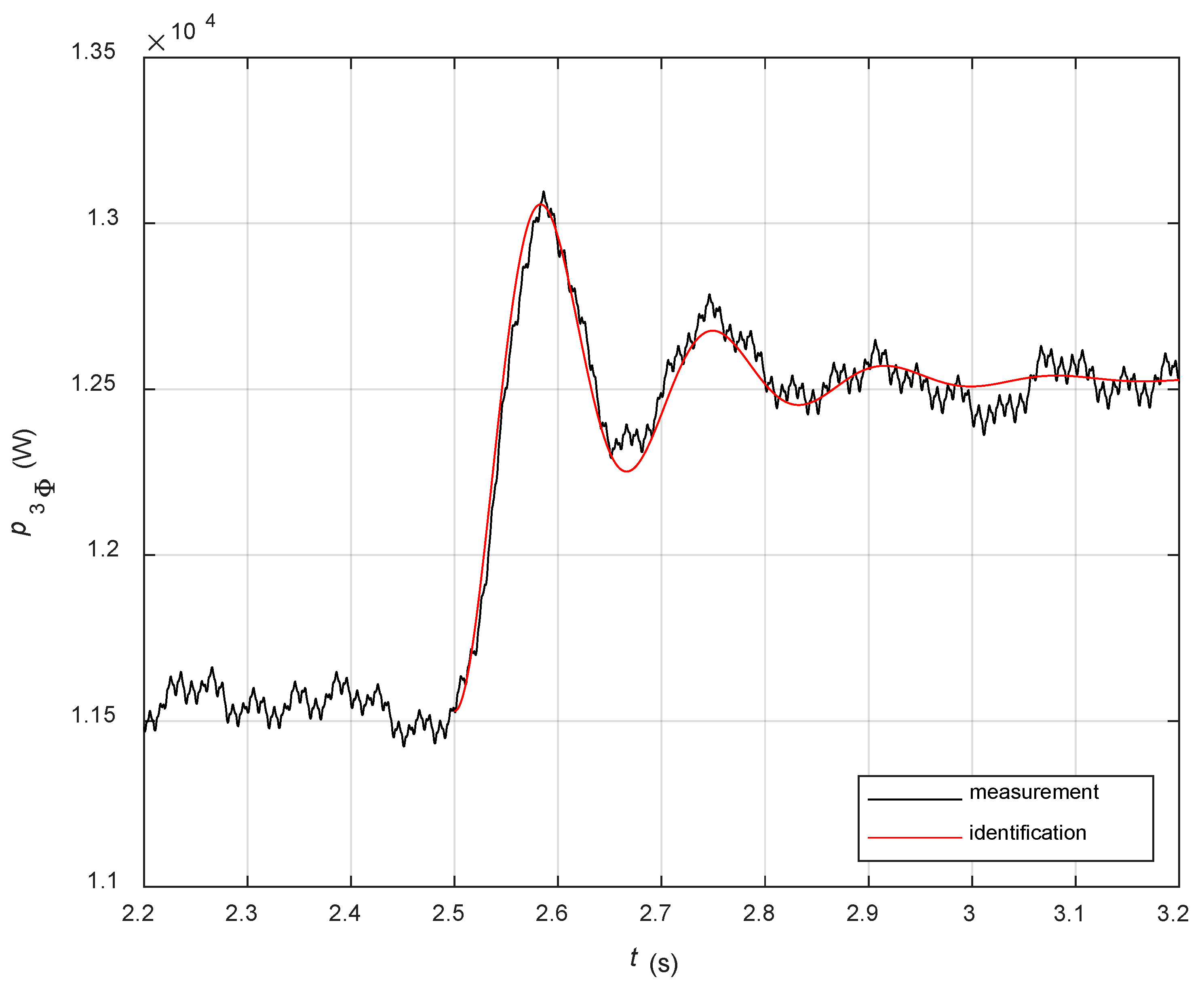
Local oscillations were analyzed throughout the entire operating range. The desired studied steady-state operating point was settled using a power amplifier and induction machine. To provoke the local oscillations, we generated a step change of the torque of the induction machine. Currents and voltages were measured, and generated powers were calculated in all phases. In the computed instantaneous 3-phase power, the local oscillation was seen clearly. It had the same time course as the step response of the second-order lag. To determine the local mode eigenvalues, we identified a second-order dynamic system with the same response as local oscillations. The second-order transfer functions were identified at different active and reactive power. The MATLAB Identification Toolbox was used to identify the transfer functions at different operating points. The poles were calculated from the c transfer functions. They corresponded to the eigenvalues of the local oscillations.

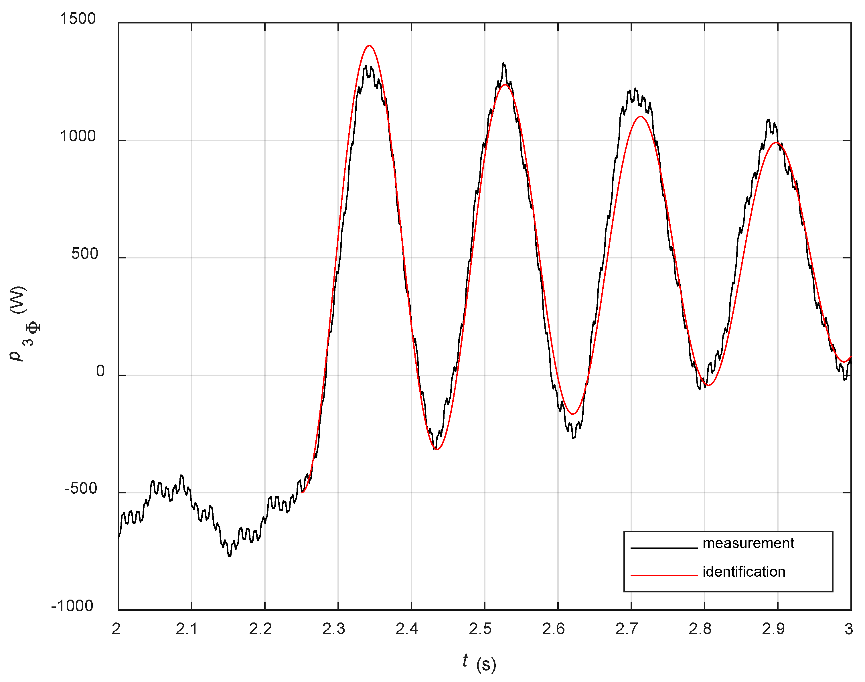
Figure 21 and Figure 22 show the time responses of the measured instantaneous 3-phase power of the laboratory synchronous generator in the vicinity of two distinctive operating points. Figure 21 presents the local oscillation in the vicinity of the operating point P = 12 kW, Q = 0 kVAr, where the oscillation was well-damped. The figure also shows the step response of the identified transfer function used to determine the eigenvalues of the local oscillation. The measured response and the simulated response of the identified model for the least-damped operating point P = 0 kW, Q = 12 kVAr are presented in Figure 22. In both cases, the simulated responses of the identified models correspond to the measured responses in the time interval after the occurrence of the step change of mechanical torque.

Measurements and identification were carried out at operating points in the entire working area.

Table 10. Real and imaginary parts of the eigenvalues, the undamped natural frequencies, and the damping ratios of the local oscillations of the laboratory synchronous generator at different operating points.

	P = 0.0 pu	P = 0.4 pu	P = 0.8 pu	P = 1.0 pu	P = 1.2 pu
Q= 0.0 pu	σ = −1.75	σ = −4.50	σ = −7.16	σ = −7.70	σ = −8.06
	ω = 22.85	ω = 27.33	ω = 34.15	ω = 37.80	ω = 41.34
	ω0 = 22.92	ω0 = 27.70	ω0 = 34.89	ω0 = 38.57	ω0 = 42.12
	ζ = 0.0764	ζ = 0.1625	ζ = 0.2053	ζ = 0.1996	ζ = 0.1915
Q= 0.5 pu	σ = −1.63	σ = −2.51	σ = −4.18	σ = −5.15	σ = −5.93
	ω = 29.22	ω = 31.22	ω = 33.47	ω = 36.43	ω = 40.06
	ω0 = 29.26	ω0 = 31.32	ω0 = 33.73	ω0 = 36.79	ω0 = 40.49
	ζ = 0.0558	ζ = 0.0801	ζ = 0.1241	ζ = 0.1400	ζ = 0.1465
Q= 1.0 pu	σ = −1.10	σ = −2.39	σ = −2.89	σ = −3.32	σ = −3.91
	ω = 34.25	ω = 36.83	ω = 37.16	ω = 37.69	ω = 39.12
	ω0 = 34.27	ω0 = 36.91	ω0 = 37.27	ω0 = 37.84	ω0 = 39.32
	ζ = 0.0321	ζ = 0.0649	ζ = 0.0776	ζ = 0.0877	ζ = 0.0996

presents the real and imaginary parts of the local mode eigenvalues, the undamped natural frequencies, and the damping ratios at measured operating points. The used base values were P_base = 12 kW and Q_base = 12 kVAr. Experimental results confirmed the main conclusions of the correlation between the operating point and the frequency and damping of local oscillations that were obtained by the numerical analysis. As expected, the values of the oscillation frequencies of the laboratory generator did not correspond to the numerically calculated limit values of power plants’ synchronous generators. The numerically obtained boundaries of the eigenvalues’ regions presented in Table A3, Table A4, Table A5 and Table A6 are valid for synchronous generators with nominal power between S_n = 1 MVA and S_n = 1000 MVA, and they deviate significantly from the eigenvalues of the laboratory synchronous generator with nominal apparent power S_n = 15 kVA.

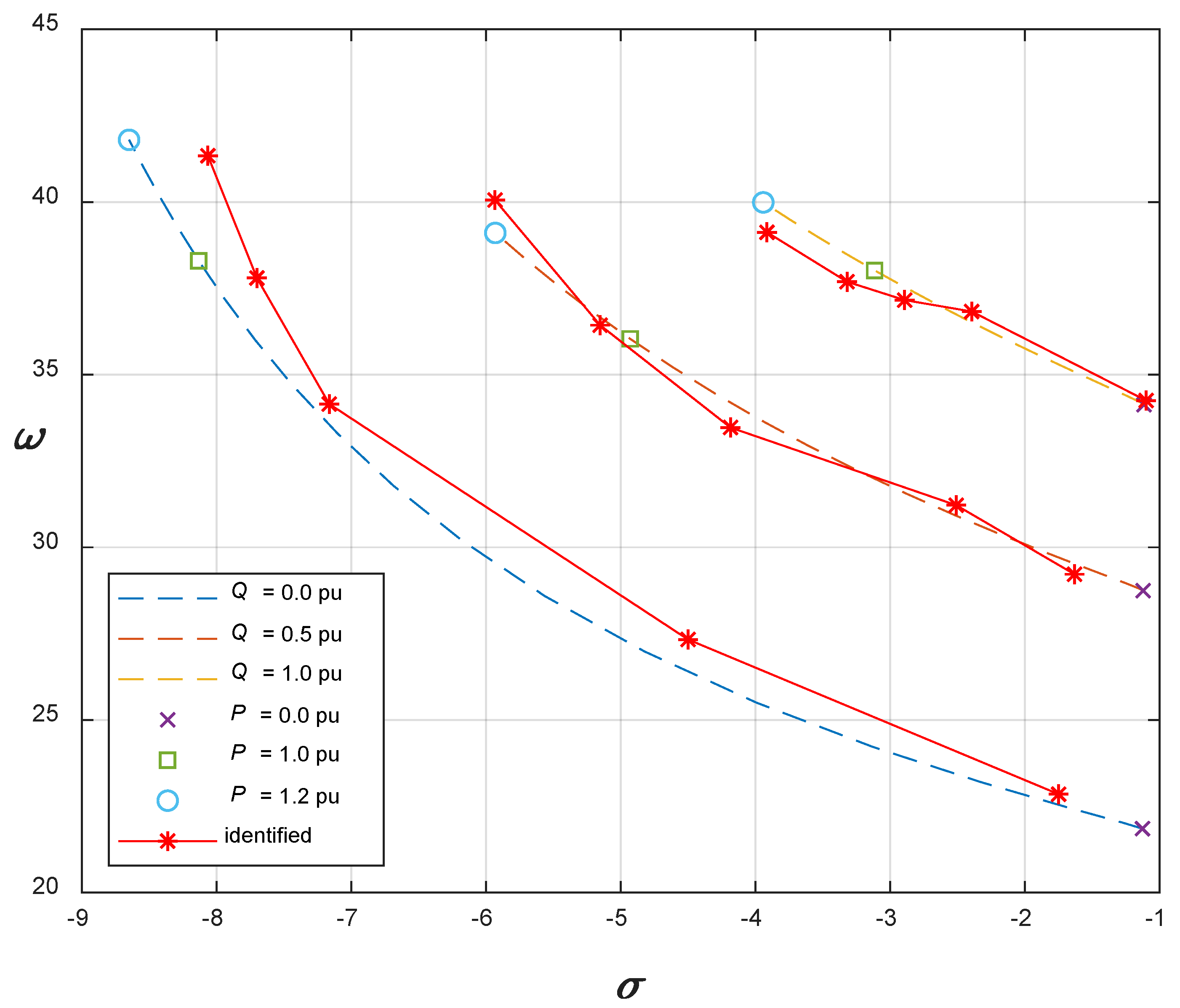
Figure 23 presents the identified local mode eigenvalues (Table 10) together with the eigenvalue loci obtained with numerical analysis of the H–P models of synchronous generators with the parameters in Table 6, Table 7 and Table 9. Active power was changed in the range of 0.0 pu to 1.2 pu at constant reactive power. The measurements were made at active power values P = 0.0 pu, P = 0.4 pu, P = 0.8 pu, P = 1.0 pu, and P = 1.2 pu, all at reactive power values Q = 0.0 pu, Q = 0.5 pu, and Q = 1.0 pu. The individual curves correspond to a constant reactive power. Local mode eigenvalues at nominal power P = 1 pu are marked on the figures with a square.

6. Conclusions

Oscillations and stability are fundamental power system problems. Oscillations cause fatigue in rotor shafts, reduce rotor life, induce power quality concerns, provoke undesirable tripping of generation units, etc. Knowledge of local oscillation modes of synchronous generators is crucial for stability analysis and instability prediction.

Local oscillations are influenced by the construction of a synchronous generator, its connection to the network and parameters, and the structure of the voltage control system and operating point. In this paper, we investigated more than 100 synchronous generators in the nominal power range from 1 MVA to 1000 MVA operating in present-day power systems. We tried to find out in what range the frequencies and dampings of local oscillations are and how individual factors affect the oscillations. Since the frequency and damping of oscillation are directly related to the eigenvalues of the mathematical model of the synchronous generator connected to the network, we carried out the study by means of eigenvalue analysis. The following conclusions were obtained:

-

Differences in the construction of the generators (slow, salient pole hydro-type synchronous generators or fast cylindrical rotor turbo-type synchronous generators) do not have a recognizable effect on the frequency and damping of local oscillations.

-

It is also not possible to draw conclusions about the influence of size (within the considered size range) on the oscillation of generators.

-

The variations of the impedance of the transmission line have a small effect on the oscillations.

-

The changing of the operating point of the synchronous generator has a very large influence on the frequency and damping of oscillations.

-

For synchronous generators of all analyzed types and sizes, the increase in generated active power results in the increase in local mode damping, and the increase in lagging reactive power results in the increase in local mode damped frequency; the operating points with the weakest damped local oscillations are at high values of reactive power and low values of active power.

-

Based on the analysis of all synchronous generators operating within the nominal conditions, we can estimate that the frequencies (f) of local oscillations of the present power plants’ synchronous generators will be in the range of 0.45–1.75 Hz (which is lower than the estimated frequencies in studies from decades ago), and the damping ratio (ζ) of local oscillations will be in the range of 0.004–0.17 (comparison of damping ratio is not possible, because no such analyses have been performed in the past).

-

An important conclusion is that the AVR affects the local oscillations immensely and can lead to instability in endangered operating areas. The AVR gain must be selected carefully so as not to cause undamped oscillations. A practical recommendation was made, which, based on the known time constant of the excitation system T_AVR and synchronous generator open-circuit time constant of a direct-axis time constants T’_d0, provides sufficiently damped local oscillations in the entire operating range (i.e., similar damping as without the AVR system).

-

The range of frequencies and dampings of local oscillations of the considered generators with AVR systems with gain calculated by the given recommendation was estimated; frequencies were in the range 0.5–1.5 Hz, and damping’s range was similar to that of synchronous generators without AVR systems.

-

The changing of the operating point of the synchronous generator with the AVR system has a large influence on the frequency and damping of oscillations.

-

The correlation between the operating points and oscillations is, for synchronous generators with AVR systems, less straightforward. While the increase of reactive power follows in all cases in the increase of undamped frequency, the increase of active power by hydro-type synchronous generators always decreases the damping of oscillations, and for turbo-type synchronous generators, it mainly increases the damping except for small values of reactive power and high values of active power. The different dependence of the eigenvalues of the different types of generators with an AVR system on the operating point is mainly due to the different values of direct-axis transient reactance.

-

It was evident from the numerical results and confirmed with a root locus diagram that for hydro- and turbo-type synchronous generators with AVR systems, the less-damped operating points represent a combination of generated small reactive power and large active power.

The sizes of frequency and damping of oscillations of the laboratory synchronous generator with nominal power S_n = 15 kVA were expected to deviate from the obtained values of generators in the nominal power range of 1 to 1000 MVA, but the experiments confirmed the discovered correlation between operating points and oscillations’ dampings and frequencies.

The presented findings answered the initial questions. The results of the study enable the estimation of expected oscillations, the evaluation of the adequacy of the AVR parameters, the distinction of local oscillations from other oscillations, the prediction of stability-problematic operation, the design and synthesis of PSS, etc. Our goal is also that engineers and scientists who work with measurements of local oscillations compare the results of their measurements with the paper’s conclusions and confirm or correct them.

References

- Kundur, P.; Paserba, J.; Ajjarapu, V.; Andersson, G.; Bose, A.; Canizares, C.; Hatziargyriou, N.; Hill, D.; Stankovic, A.; Taylor, C.; et al. Definition and Classification of Power System Stability IEEE/CIGRE Joint Task Force on Stability Terms and Definitions. IEEE Trans. Power Syst. 2004, 19, 1387–1401. [Google Scholar] [CrossRef]
- Ritonja, J. Adaptive stabilization for generator excitation system. COMPEL—Int. J. Comput. Math. Electr. Electron. Eng. 2011, 30, 1092–1108. [Google Scholar] [CrossRef]
- Haes Alhelou, H.; Hamedani-Golshan, M.E.; Njenda, T.C.; Siano, P. A Survey on Power System Blackout and Cascading Events: Research Motivations and Challenges. Energies 2019, 12, 682. [Google Scholar] [CrossRef] [Green Version]
- Kundur, P. Power System Stability and Control; Electric Power Research Institute, McGraw-Hill, Inc.: New York, NY, USA, 1994. [Google Scholar]
- Heffron, W.G.; Phillips, R.A. Effect of a Modern Amplidyne Voltage Regulator on Underexcited Operation of Large Turbine Generators [Includes Discussion]. Trans. Am. Inst. Electr. Eng. Part III Power Appar. Syst. 1952, 71, 692–697. [Google Scholar] [CrossRef]
- Tan, S.; Geng, H.; Yang, G. Phillips-Heffron model for current-controlled power electronic generation unit. J. Mod. Power Syst. Clean Energy 2017, 6, 582–594. [Google Scholar] [CrossRef] [Green Version]
- Zaker, B.; Gharehpetian, G.B.; Karrari, M. Small signal equivalent model of synchronous generator-based grid-connected microgrid using improved Heffron-Phillips model. Int. J. Electr. Power Energy Syst. 2019, 108, 263–270. [Google Scholar] [CrossRef]
- Ritonja, J.; Petrun, M.; Cernelic, J.; Brezovnik, R.; Polajzer, B. Analysis and Applicability of Heffron–Phillips Model. Elektron. Elektrotech. 2016, 22, 3–10. [Google Scholar] [CrossRef] [Green Version]
- Karrari, M.; Malik, O.P. Identification of Heffron-Phillips model parameters for synchronous generators using online measurements. IEE Proc.—Gener. Transm. Distrib. 2004, 151, 313–320. [Google Scholar] [CrossRef]
- Soliman, M.; Westwick, D.; Malik, O.P. Identification of Heffron–Phillips model parameters for synchronous generators operating in closed loop. IET Gener. Transm. Distrib. 2008, 2, 530–541. [Google Scholar] [CrossRef]
- Larsen, E.V.; Swam, D.A. Applying power system stabilizers, Part I, II and III. IEEE Trans. Power Appar. Syst. 1981, 100, 3017–3033. [Google Scholar] [CrossRef]
- Rogers, G. Demystifying power system oscillations. IEEEE Comput. Appl. Power 1996, 9, 30–35. [Google Scholar] [CrossRef]
- Follum, J.D.; Tuffner, F.K.; Dosiek, L.A.; Pierre, J.W. Power System Oscillatory Behaviors: Sources, Characteristics, & Analyses; North American SynchroPhasor Initiative, Office of Electricity Delivery and Energy Reliability, United States Department of Energy: Washington, DC, USA, 2017.
- Deng, J.; Xia, N.; Yin, J.; Jin, J.; Peng, S.; Wang, T. Small-Signal Modeling and Parameter Optimization Design for Photovoltaic Virtual Synchronous Generator. Energies 2020, 13, 398. [Google Scholar] [CrossRef] [Green Version]
- Yuan, S.; Hao, Z.; Zhang, T.; Yuan, X.; Shu, J. Impedance Modeling Based Method for Sub/Supsynchronous Oscillation Analysis of D-PMSG Wind Farm. Appl. Sci. 2019, 9, 2831. [Google Scholar] [CrossRef] [Green Version]
- Yang, B.; Li, G.; Tang, W.; Hu, A.; Zhang, D.; Wu, Y. Energy Storage System Controller Design for Suppressing Electromechanical Oscillation of Power Systems. Appl. Sci. 2019, 9, 1329. [Google Scholar] [CrossRef] [Green Version]
- Tchawou Tchuisseu, E.B.; Gomila, D.; Brunner, D.; Colet, P. Effects of dynamic-demand-control appliances on the power grid frequency. Phys. Rev. E 2017, 96, 022302. [Google Scholar] [CrossRef] [PubMed] [Green Version]
- Dobson, I.; Carreras, B.A.; Lynch, V.E.; Newman, D.E. Complex systems analysis of series of blackouts: Cascading failure, critical points, and self-organization. Chaos Interdiscip. J. Nonlinear Sci. 2007, 17, 026103. [Google Scholar] [CrossRef] [PubMed]
- Carreras, B.A.; Tchuisseu, E.B.T.; Reynolds-Barredo, J.M.; Gomila, D.; Colet, P. Effects of demand control on the complex dynamics of electric power system blackouts. Chaos Interdiscip. J. Nonlinear Sci. 2020, 30, 113121. [Google Scholar] [CrossRef] [PubMed]
- Wu, Q.; Huang, Y.; Li, C.; Gu, Y.; Zhao, H.; Zhan, Y. Small Signal Stability of Synchronous Motor-Generator Pair for Power System with High Penetration of Renewable Energy. IEEE Access 2019, 7, 166964–166974. [Google Scholar] [CrossRef]
- Demello, F.P.; Concordia, C. Concepts of Synchronous Machine Stability as Affected by Excitation Control. IEEE Trans. Power Appar. Syst. 1969, PAS-88, 316–329. [Google Scholar] [CrossRef] [Green Version]
- Ritonja, J.; Dolinar, D.; Polajžer, B. Adaptive and robust controls for static excitation systems. COMPEL—Int. J. Comput. Math. Electr. Electron. Eng. 2015, 34, 864–881. [Google Scholar] [CrossRef]
- Anderson, P.M.; Fouad, A.A. Power System Control and Stability, 2nd ed.; John Wiley & Sons Inc.: Piscataway, NJ, USA, 2003. [Google Scholar]
- IEEE Guide for Synchronous Generator Modeling—Practices and Applications in Power System Stability Analyses. In IEEE Standard 1110; IEEE: New York, NY, USA, 2002.
- Rotating Electrical Machines—Methods for Determining Synchronous Machine Quantitites from Tests. In IEC Standard 60034-4; IEC: Geneva, Switzerland, 2008.
Figure 1.
Eigenvalue loci of local mode of 9-MVA hydro-type synchronous generator without AVR.
Figure 2.
Eigenvalue loci of local mode of 12-MVA hydro-type synchronous generator without AVR.
Figure 3.
Eigenvalue loci of local mode of 158-MVA hydro-type synchronous generator without AVR.
Figure 4.
Eigenvalue loci of local mode of 615-MVA hydro-type synchronous generator without AVR.
Figure 5.
Eigenvalue loci of local mode of 25-MVA turbo-type synchronous generator without AVR.
Figure 6.
Eigenvalue loci of local mode of 160-MVA turbo-type synchronous generator without AVR.
Figure 7.
Eigenvalue loci of local mode of 911-MVA turbo-type synchronous generator without AVR.
Figure 8.
Eigenvalue loci of local mode of a 158-MVA hydro-type synchronous generator where transmission line impedance was reduced to 50% of the nominal (real) impedance (comparable with Figure 3).
Figure 9.
Block diagram of the studied AVR system.
Figure 10.
Influence of exciter and AVR gain kAVR on the local mode eigenvalue of the hydro-generator with nominal power 158 MVA for nominal operating point S = 158 MVA, cos φ = 0.9.
Figure 11.
Eigenvalue loci of the local mode of 9-MVA hydro-type synchronous generator with AVR.
Figure 12.
Eigenvalue loci of the local mode of 12-MVA hydro-type synchronous generator with AVR.
Figure 13.
Eigenvalue loci of the local mode of 158-MVA hydro-type synchronous generator with AVR.
Figure 14.
Eigenvalue loci of the local mode of 615-MVA hydro-type synchronous generator with AVR.
Figure 15.
Root locus diagrams of local mode eigenvalue for a hydro-type synchronous generator with nominal power 158 MVA for operating points: (i) P = 0.5 pu, Q = 0.0 pu, (ii) P = 1.0 pu, Q = 0.0 pu and (iii) P = 1.2 pu, Q = 0.0 pu.
Figure 16.
Eigenvalue loci of local mode of 25-MVA turbo-type synchronous generator with AVR.
Figure 17.
Eigenvalue loci of local mode of 160-MVA turbo-type synchronous generator with AVR.
Figure 18.
Eigenvalue loci of local mode of 911-MVA turbo-type synchronous generator with AVR.
Figure 19.
Eigenvalue loci of local mode of a 158-MVA hydro-type synchronous generator with AVR system at reactive power Q = 0.6 pu, and active power values from P = 0.0 pu to P = 1.2 pu for different values of the direct-axis transient reactance xd’.
Figure 20.
Laboratory experimental system.
Figure 21.
Time response of the instantaneous three-phase power of the laboratory synchronous generator Sn = 12 kV in the vicinity of the operating point P = 12 kW, Q = 0 kVAr on the step change of mechanical torque corresponding to mechanical power change from 11.5 kW to 13.5 kW compared with the identified local oscillation.
Figure 22.
Time response of the instantaneous three-phase power of the laboratory synchronous generator Sn = 12 kV in the vicinity of the operating point P = 0 kW, Q = 12.0 kVAr on the step change of mechanical torque corresponding to mechanical power change from −0.5 kW to 0.5 kW compared with the identified local oscillation.
Figure 23.
Eigenvalue loci of the local mode of the laboratory synchronous generator Pn = 12 kW obtained with numerical analysis of an H–P model and with identification of the measured time responses of the oscillations conducted with step changes of the mechanical torque.