
Three-Dimensional Human Head Reconstruction Using Smartphone-Based Close-Range Video Photogrammetry


Department of Electronic Systems, Vilnius Gediminas Technical University (VILNIUS TECH), 03227 Vilnius, Lithuania
*
Author to whom correspondence should be addressed.
Appl. Sci. 2022, 12(1), 229; https://0-doi-org.brum.beds.ac.uk/10.3390/app12010229
Submission received: 17 November 2021
/
Revised: 20 December 2021
/
Accepted: 22 December 2021
/
Published: 27 December 2021
(This article belongs to the Special Issue Machine Learning Application in Human Motion Tracking)
Abstract
:Creation of head 3D models from videos or pictures of the head by using close-range photogrammetry techniques has many applications in clinical, commercial, industrial, artistic, and entertainment areas. This work aims to create a methodology for improving 3D head reconstruction, with a focus on using selfie videos as the data source. Then, using this methodology, we seek to propose changes for the general-purpose 3D reconstruction algorithm to improve the head reconstruction process. We define the improvement of the 3D head reconstruction as an increase of reconstruction quality (which is lowering reconstruction errors of the head and amount of semantic noise) and reduction of computational load. We proposed algorithm improvements that increase reconstruction quality by removing image backgrounds and by selecting diverse and high-quality frames. Algorithm modifications were evaluated on videos of the mannequin head. Evaluation results show that baseline reconstruction is improved 12 times due to the reduction of semantic noise and reconstruction errors of the head. The reduction of computational demand was achieved by reducing the frame number needed to process, reducing the number of image matches required to perform, reducing an average number of feature points in images, and still being able to provide the highest precision of the head reconstruction.
1. Introduction
Three-dimensional modeling of the human head has a wide range of applications. Three-dimensional data of the head, with extension to the whole body, are widely used in clinical, industrial, anthropological, forensic, sports, commercial, and entertainment areas. Medical applications of 3D scanning may be divided into four groups: epidemiology, diagnosis, treatment, and monitoring [1,2]. The 3D measurements can benefit cranial deformation studies [3,4,5,6], diagnosis, craniofacial information analysis [7], and evaluation of the effects of orthotic helmets [8]. Models and 3D visualizations allow measurements to be performed for planning a surgical intervention, assess surgical outcomes, measure changes after surgeries, forecast the result of a facial plastic/cosmetic surgery, document clinical cases, compare pre-treatment and post-treatment models [9], perform more accurate orthodontics diagnoses [10], and achieve better dental reconstruction results [11]. In biomedical engineering, anthropometrical measurements help to design prosthesss [12] and allow for the rapid prototyping of customized prostheses. The manufacturing of medical products has to be based on population anthropometrical studies so that medical equipment perfectly suits the physical characteristics of patients [13]. Head 3D modeling may be used for the documentation of research, registering EEG electrode positions [14,15,16], collection of anthropometric data [17,18,19,20,21], and defining normal head parameters [22]. Non-medical fields of 3D head modeling applications include computer animation, movies and animation, security, teleconferences, and virtual reality, forensic identification [23], behavior research (perceptions of attractiveness), identifying human facial expressions, and sculpture [24]. Another large group of applications are found in industry: design of headwear products, such as helmets, headgear, glasses, and headphones [25,26]; optimization of wearable product comfort and function [27,28,29], perform better ergonomic design of human spaces, simulate the wearing of clothes [30,31], and create products that take into account ergonomics [27,32], model and predict respirator size and fit [25,33,34].
There are several types of imaging techniques to create 3D models: laser line systems [35], structured light systems [36], close-range photogrammetry [37,38,39], and radio-wave-based image capturing systems [40]. Image-based reconstruction and modeling of scene [41,42,43], objects [44] and processes [45,46] is a widely accessible technique in terms of price for gathering information [1,47,48]. The complexity of usage of such technologies mostly depends on algorithms and user interface design. Three-dimensional objects may be reconstructed by fitting mathematical models to the collected image data [49,50]. However, the model is required, and it should be adequate to represent a range of variations the modeled object may possess. Therefore, the most popular technique for estimating three-dimensional structures from two-dimensional image sequences is Structure from Motion (SfM) [51,52,53,54]. The means of object modeling that is easily accessible to ordinary users is based on handheld devices, such as smartphones [55,56]. Smartphone-based close-range digital photogrammetry would be the desired way for modeling objects at home. Photogrammetry using ordinary consumer-grade digital cameras can provide a cost-effective and sufficiently accurate solution for creating 3D models of the head as new smartphones come equipped with higher quality cameras. The most common application of head modeling for home users could be the acquisition of head anthropometric data in order to select the appropriate size of headwear products. The other application could be trying out head apparel.
The construction process of the head 3D model for the home user must be fully automatic. The software tool is only allowed to give the user simple directions to correct their actions if they lead to a model of unsatisfactory quality. The simplest way for the user to collect a set of their head images would be to record a selfie video covering as many various views of their head as possible. Using a general-purpose 3D reconstruction algorithm, automatic reconstruction of the head may suffer from the non-static scene and various image photometric distortions.
This work proposes a methodology for the improvement of 3D head reconstruction, primarily from selfie videos, by increasing reconstruction quality and reducing the number of required computations.
The novelty and contributions of this work can be summarized as follows:
- Adaptation of a general-purpose 3D reconstruction algorithm to create head 3D point clouds from selfie videos;
- Achieved an increase of 3D head reconstruction quality by removal of background information and by selecting a subset of best quality frames from the full set of frames;
- Presented and compared methods for the selection of the highest quality frames;
- Performed comparative evaluation of feature sources (layer of convolutional neural network (CNN)) and dimensionality-reduction (DR) techniques used to order images by similarity in and with the purpose to predict the image’s relative pose;
- Presented comparative results of the 3D head reconstruction improvements using mannequin head videos.
Overview of the general-purpose 3D reconstruction algorithm and its proposed modifications to improve the 3D head reconstruction process is presented in Figure 1.
2. Materials and Methods
In this section, we describe the general-purpose 3D reconstruction algorithm and its shortcomings in using it for head reconstruction; we create a methodology for the improvement of 3D head reconstruction and use it to propose changes for the general-purpose 3D reconstruction algorithm; we present the rationale behind the proposed algorithm improvements and their implementation solutions; we describe the experimental data collection process, creation of head reference and test models; and outline the evaluation process of reconstruction algorithms.
2.1. 3D Reconstruction Algorithms
2.1.1. Requirements for 3D Reconstruction Algorithm from Usability Viewpoint
Shortcomings of the general-purpose 3D reconstruction algorithm in head modeling arise from the specifics of how the initial data (mostly it will be a selfie video) is collected and the kind of final reconstruction (model) we want to create. We aim to create a head model that is without semantic noise, i.e., the reconstructed scene contains only the head as an object and no other points that would belong to non-head objects. Such a model would not require any automatic or manual postprocessing, which would not necessarily be accurate and successful enough, but also, the model would be more appropriate for making measurements and for visualization purposes. Moreover, we want to create a model that has as few reconstruction errors as possible. Thus, we want the model to be high quality, i.e., having a low level of semantic noise and a low level of reconstruction errors.
Semantic noise in the reconstructed scene will exist as everything will be reconstructed, not just the object of interest. The bad thing is that the noise will interfere with measurements or disturb visualization. It would be possible to edit or filter a point cloud, but this is a complicated task and does not guarantee a quality result. The other requirement for the data collection process in order for the general-purpose 3D reconstruction algorithm worked properly is that the scene must be static. However, if we are capturing our own head (most of the cases) or another person’s head, it will not be possible to ensure that everything in the scene is fixed and does not move. Facial emotions during filming for 30–90 s could be controlled, but staying still so that there are no background changes is practically impossible. During reconstruction, a changing background would interfere with the reconstruction of the object, as richer textures in the background may result in a more accurate reconstruction of the object’s environment, but not the object itself. A partial solution could be filming in the environment with a patternless, textureless background, but the user would need a background that spans almost entirely around them (such as a corner between walls of the same color) such a place may be hard to locate. Therefore, an easier solution would be to remove the background in the photos so that the background would not have influence.
Another need for adjustment of the reconstruction algorithm is the specialization for working with videos. It is more convenient to film one’s head than photograph it, especially if a person wants to image their head. Making selfie videos using a smartphone is more convenient than taking many selfie photos because, during the shooting, a user needs to keep the face as still as possible. Moreover, a user should not move the handheld camera too fast during filming in order to minimize image distortions, such as motion blur and rolling shutter. Slow camera movement during filming will create many similar frames, so it is not helpful to use all frames for the reconstruction. Due to the excessive number of repetitive images, the volume of calculations for the reconstruction will increase significantly, but the accuracy will practically not improve. It would be helpful to detect and remove from the reconstruction process frames that have highly redundant information. Among the many frames, there will also be low-quality ones, where the face is slightly outside the frame or affected by motion blur distortions due to a shaky hand. Such frames also need to be removed. Thus, the basic reconstruction algorithm has been supplemented with actions to remove unnecessary frames and, as a result, lower reconstruction errors.
2.1.2. Methodology for Improvement of 3D Head Reconstruction
Here, we propose a methodology for the improvement of 3D head reconstruction. We seek reconstruction improvement by increasing the reconstruction quality and reducing the number of required computations. We define the model quality by the amount of semantic noise and reconstruction errors—the higher level of noise and errors, the lower the quality of the model. The methodology is a list of possible solutions that systematically originated from the factors that negatively affect the reconstruction process and quality of the head model.
We have summarized the factors that may negatively affect the reconstruction process and quality of the reconstructed head model (discussed in previous Section 2.1.1):
- Changing background—due to the movement of the head in respect of the background or existence of other moving objects in the background;
- Motion blur and rolling shutter distortion—due to low light conditions and faster movement of the camera, shivering of hand;
- Defocus distortions—if the camera focuses on background objects;
- Head out of frame limits—stumbles making selfie videos;
- Too many frames—due to the inefficient design of camera positioning around the head and, as a consequence, acquired long recording (excess of redundant frames only slows down reconstruction process).
These key modifications of the general-purpose 3D reconstruction algorithm should improve 3D head reconstruction from selfie videos by weakening factors that negatively affect the reconstruction process and quality of the model:
- Elimination of image background—suppresses the negative influence of the changing background to the reconstruction process; reduces the amount of semantic noise; background elimination frees from computations in the background region of the image;
- Selection of the highest quality frames—as a result, reconstruction errors are reduced because images with motion blur, defocus distortions, and images, where the head is out of frame limits, are removed; reduces the number of frames that are redundant, so the computational load is reduced; removal of redundant frames enables moving the camera slowly while capturing in order to reduce motion blur and rolling shutter distortions.
Specifics of the implementation solutions of these modifications will be presented and discussed in Section 2.1.4.
2.1.3. Baseline Algorithm
The default Photogrammetry Pipeline from the AliceVision Meshroom software (version 2021.1.0) [57] with small adjustments was used as a general-purpose 3D reconstruction algorithm, and in the comparative evaluation of the algorithms it represented the baseline algorithm.
The reasons that led to the choice of the Meshroom were its functionality (features), popularity among users, acceptable reconstruction quality, being open-source, active development, the possibility to access and modify intermediate data, modular structure, and command-line interface. In order to evaluate the proposed modifications of the 3D reconstruction pipeline, a flexible environment for experimentation was needed. Meshroom provides a means to adapt the pipeline through its customizable workflow and/or by accessing intermediate data. It is easy to intervene in the workflow with custom data processing steps. It is worth mentioning that there exist a number of other photogrammetry software as free/open-source and commercial packages. Free/open-source applications for SfM [58]: COLMAP [59,60], OpenMVG [61], VisualSFM [62], Regard3D [63], OpenDroneMap (ODM) [64], MultiViewEnvironment (MVE) [65], MicMac [66]. Commercial solutions [67]: 3Dflow 3DF Zephyr [68], Agisoft Metashape [69], Autodesk ReCap [70], Bentley ContextCapture [71], CapturingReality RealityCapture [72], PIX4Dmapper [73], PhotoModeler [74], DroneDeploy [75], OpenDroneMap WebODM [76], Trimble Inpho [77], and Elcovision 10 [78].
The adjustments and their justification are following:
- Describer Types in FeatureExtraction node were changed from sift to a combination of sift_upright and akaze_ocv—the first change because the camera is not rotated during the capture and hence the feature orientation may be fixed; the second change adds more diverse features to increase matching robustness;
- In FeatureMatching node parameters, Cross Matching and Guided Matching, were enabled—to increase matching robustness;
- The default single StructureFromMotion node was changed to a sequence of two StructureFromMotion nodes with the following different settings—in the first StructureFromMotion node, the value of parameter Min Input Track Length was changed from 2 to 3, and the value of parameter Min Observation For Triangulation was changed from 2 to 4. In the second StructureFromMotion node, the parameter Lock Scene Previously Reconstructed was enabled, and the value of parameter Min Observation For Triangulation was changed from 2 to 3. Such setup increases the number of reconstructed cameras and reduces the noise in the point cloud;
- Only the sparse reconstruction part of the whole reconstruction pipeline was used, so the sparse point cloud from the last StructureFromMotion node was used as the test model in the evaluation.
This baseline algorithm in the context of the generalized 3D reconstruction pipeline (Figure 1) consists of the steps: 1. Frame extraction from video; 2. Camera initialization; 6. Feature point detection; 8. Feature description; 9. Image matching; 10. Feature (descriptor) matching; 11. Structure from motion (sparse reconstruction). Formally, 5. Frame selection step was also performed in a simple way because a large amount of extracted frames from the video was reduced 3 to 4 times, depending on the initial frame count, so that the remaining frame count was near 400. The set of frames was reduced by taking every third or fourth frame. All selected frames from the videos were sent to the 3D reconstruction algorithm without any preprocessing. Any geometric distortions, for instance, due to camera optics, were corrected during the bundle adjustment process of 11. Structure from motion step when the extrinsic and intrinsic parameters of all cameras, together with the position of all 3D points, are being refined.
The following are the essential steps of the Meshroom’s StructureFromMotion node [57,79], which is an incremental algorithm, and are concealed under the 11. Structure from motion step (Figure 1): 1. Fusion of all feature matches between image pairs into tracks; 2. Selection of the initial image pair and estimation of the fundamental matrix between these two images; 3. Triangulation of the feature points from the image pair; 4. Next best view selection; 5. Estimation of a new camera pose (robust RANSAC framework is used to find the pose of the new camera, and nonlinear optimization is performed to refine the pose); 6. Triangulation of the new points; 7. Performing Bundle Adjustment to refine the positions of 3D points, extrinsic and intrinsic parameters of the reconstructed cameras; 8. Looping from the fourth to eighth step until no new views are localized.
When introducing algorithm improvements according to the presented methodology (Section 2.1.2), adjustments presented here are kept.
2.1.4. Algorithms with Proposed Modifications
In the previous sections, we discussed the requirements for 3D head reconstruction algorithms from selfie videos from the usability viewpoint (Section 2.1.1). Later, the methodology for the improvement of 3D head reconstruction was proposed (Section 2.1.2). The methodology consists of key modifications of the general-purpose 3D reconstruction algorithm to improve 3D head reconstruction from selfie videos. Here, we introduce implementations of algorithm improvements according to the presented methodology.
All modifications are introduced gradually in order to be able to compare their influences on the reconstruction process. It resulted in three major branches of modified reconstruction algorithms and a total of six minor branches. The summary of the 3D head reconstruction algorithms, which will be explored in this work, is presented in Table 1. The main modifications followed from the proposed methodology in Section 2.1.2, which specifies that the elimination of the image background and selection of the highest quality frames should be performed.
Background Elimination
The first branch of the baseline algorithm is created by adding image background elimination and is labeled as Pipeline 2 with sub-branches {a|b} (Figure 1). The sub-branches differ in one change of a parameter value: the value of Describer Density parameter in the FeatureExtraction node in the case of variant (a) is normal, and in case of variant (b) is high. Background elimination is implemented as 7. Initial feature point selection following the 6. Feature point detection step of the generalized 3D reconstruction pipeline. The initial feature point selection (or elimination of unnecessary points) process requires information about the bounds of the main object, i.e., the head. This information is provided by the 3. Head detection step of the generalized 3D reconstruction pipeline. The background elimination is implemented through feature point selection—it was a more reasonable way to integrate this step with the Meshroom pipeline. Simple masking of the background in the initial images would lead to spurious feature points on the edge of the background cutting.
Head Detection
A convolutional neural network (CNN) single-shot detector (SSD) [80] is used for head detection [81] in the images (Figure 2). The model adopted in this research was developed by the authors of LAEO-Net [82]. The model’s suitability for the task was evaluated by manually revising the head detection results on the collected dataset of 19 videos. The bounding box (BBox) that indicates the boundaries of the head in the image will be used to remove those feature points that are behind the boundary of the head. During the head detection, not only data on the location of the head in the image are collected, but additionally intermediate results from the intermediate convolutional layers of the CNN (Figure 3). Data from the feature layers are used as features to describe the image patch containing the head. By using these features, the frames can be grouped according to similarity. This grouping will be exploited later in redundant frame dropping.
Frames Selection Methods
Two goals may be achieved simultaneously by performing frame selection—removing redundant data from the dataset to reduce the dataset and, as a result, reduce the computational load, and removing images that are low quality due to motion and defocus blur. We implemented and tested two different methods for frame selection.
The first method is a straightforward extension of the simplest frame reduction strategy where every N-th frame is selected. The modification is made by integrating image quality estimates into the frame selection process. Image quality is estimated for every frame, and instead of selecting every N-th frame, the frame with the highest quality from N consecutive frames is selected. The image quality estimation method is presented below. The second branch of the baseline algorithm is created by adding the simplest frame reduction strategy together with the previously added image background elimination and is labeled as Pipeline 3 with sub-branches {a|b} (Table 1). This frame reduction strategy is implemented as 4. Image quality estimation and 5. Frame selection steps of the generalized 3D reconstruction pipeline (Figure 1).
The second frame selection method is more universal. It selects a predefined number of frames from a full set of frames, so the images may have come from an unordered image set—from a video with chaotic camera trajectories, from different videos, or collected as photographs. To achieve a satisfactory object 3D reconstruction result, we need images that are evenly spaced and cover a wide area around the object, and we need to additionally include a spacing term in the image quality estimate. The image quality estimation method in combination with spatial image ordering is presented below. The third branch of the baseline algorithm is created by adding the frame reduction strategy, which performs image ordering by similarity and later selects the best quality images in image groups, and is labeled as Pipeline 4 with sub-branches {a|b} (Table 1). This frame reduction strategy is implemented as 4. Image quality estimation and 5. Frame selection steps of the generalized 3D reconstruction pipeline (Figure 1).
Image Quality Estimation
The image sharpness metric was used as an estimate of image quality for the frame selection. This algorithm implements the 4. Image quality estimation step of the generalized 3D reconstruction pipeline (Figure 1) when Pipeline 3{a|b} is selected (Table 1).
Key algorithm steps for image sharpness estimation:
- Detect the head region defined by BBox (it is already detected in the background removal step);
- Calculate Region of Interest (RoI) parameters: define the size of square as the largest edge of head BBox;
- Crop RoI part and resize to px image patch;
- Filter patch using Laplacian of Gaussian (LoG) filter ( filter size, );
- Calculate the variance of filtered patch;
- A larger variance represents a higher image sharpness.
Frame Pose Prediction by Image Similarity Ordering
Frame pose prediction by ordering images according to similarity is a crucial step to create a subset of images that covers a wide area around the object and contains evenly spaced images. Here, we define image similarity in terms of camera pose in 3D space. Pictures or frames having similar poses will likely be similar if the scene is static. Image ordering by similarity is a proxy task to predict the relative poses of the frames. Having relative poses, we could select the best quality image from the image group corresponding to a predefined region of the surrounding space. To imitate image ordering in 3D space or in 2D space, if we assume that the camera keeps an approximately constant distance from the head, we would like to get 3D or 2D embeddings of the images.
To get image embeddings in 2D or 3D, a possible solution would be to collect multidimensional feature vectors that describe images containing a head from the CNN that were used to detect heads in the images and later to reduce dimensionality. The CNN model is trained to detect heads, so the features extracted by the network should serve as good descriptors of the head image patch. Additionally, it would be the third task where the same CNN model serves, i.e., head detection for initial feature point selection, for image quality evaluation as the RoI provider, and here, as a feature extractor for image description. Feature vectors can be taken from any feature layer at any (row, column) position. The position (row, column) is determined from the results of the same network—the center of the detected BBox of the head (Figure 3). A suitable feature layer may be suggested according to the size of the receptive fields of the units and from the units that the feature layer has. The further the feature layer starts from the input, the larger the receptive fields of the units of that layer are. The size of the receptive field will determine what part of the image the extracted feature vector describes. We want to compare, by similarity only, the image regions that semantically represent the head. Intuitively, the size of the receptive field should be such that it spans the region of the head in the image. However, we will perform experiments to select the feature layer that is most helpful to provide feature vectors (Table 2).
Particular feature vector (from a specific layer, certain (row, column) location) will mostly be shift invariant, but not scale or rotation invariant. Shift invariance was achieved by using information about the detected center of the head BBox to determine the (row, column) location of the feature vector. Rotation invariance is not as important because during the short video capture, the camera may be used without large tilt rotations. Scale invariance probably would be slightly needed if we made a selfie video using an outstretched hand. If the video was made with a strongly changing distance from the camera to the head, or if we use frames from different videos, the scale of the head in separate frames may differ. This can lead to the situation where feature vectors differently describe the same object due to the change of the object’s size. Scale invariance may be achieved by performing double-pass head detection—after the first run, the detected BBox is used to crop the image region with the head, and the cropped image is passed to the model for the second detection. We will perform experiments to check what changes in the results of image similarity order may be achieved by adding a second pass.
The extracted feature vectors are multidimensional. The dimensionality of the feature vector is equal to the number of channels in the feature layer. In order to get image embeddings in 2D or 3D, we must reduce the dimensionality of the feature vectors. A set of dimensionality techniques will be compared in order to select the one that, combined with the selected type of feature vector, will provide the best-ordered images by similarity. The goodness of the image order will be measured by the percentage overlap of the two sets that contain the closest images to the target image. It means that for each image, we find the closest group of images in space (according to known image poses), and we find the closest (most similar) images according to the extracted feature vectors. The percentage overlap of these sets gives the estimate of the goodness of the image order. As the ground truth poses the images, we use the reconstructed poses using Pipeline 2b (Table 1).
The following dimensionality-reduction techniques will be experimentally compared for suitability for image ordering by similarity.
- t-Distributed Stochastic Neighbor Embedding (t-SNE);
- Stochastic Neighbor Embedding (SNE);
- Classical multidimensional scaling (MDS);
- Principal Component Analysis (PCA);
- Probabilistic PCA;
- Kernel PCA;
- Linear Discriminant Analysis (LDA);
- Factor Analysis (FA);
- Sammon mapping;
- Diffusion maps;
- Stochastic Proximity Embedding (SPE);
- Gaussian Process Latent Variable Model (GPLVM);
- Neighborhood Components Analysis (NCA);
- Large-Margin Nearest Neighbor (LMNN).
Implementations of the techniques were used from the Matlab Toolbox for Dimensionality Reduction (https://lvdmaaten.github.io/drtoolbox accessed on 9 August 2021) [83,84].
The best performing combination of the feature type and dimensionality-reduction technique will be used for frame selection in Pipeline 4.
Key algorithm steps for frame selection in Pipeline 4:
- Extract feature vectors describing the regions of images that contain the head;
- Perform dimensionality reduction using the selected technique;
- Define a grid in the low-dimensional feature space that divides the space into uniform cells. A step size of the grid depends on the total frame number we want to select (in this research, the target was 200 frames);
- In each cell, if several frames get into the same cell, only the image with the largest sharpness gets kept.
2.2. Creation of the Head Models
Getting the evaluation results of reconstruction algorithms is based on the comparison of test and reference models. For objective evaluation, it is crucial to create a high-quality reference model. The creation of test models is directed by the algorithms we seek to compare. Therefore, the construction processes of reference and test models have differences. The reference and test models were constructed using the specifically collected data. The collection process of the video and photo data is described in Section 2.5.
2.2.1. Reference Model Creation
The goal of the reference model creation task is to reconstruct the mannequin’s head with the highest precision. This 3D model should have the lowest level of semantic noise and the lowest level of reconstruction errors. Semantic noise (any points belonging to the non-head class) may be reduced by removing background information from the images. Possible reconstruction errors may be reduced by making and selecting the highest quality images. The creation of the reference head model does not have time or tool selection constraints or any manual work quota. After the photos were taken, they were manually edited to remove the background. The background is removed approximately by trying to select as much as possible of it without damaging parts of the head. The photos were also reviewed to avoid poor-quality photos with poor focus and motion blur distortions. A total of 187 photos were selected for reference model reconstruction. Three-dimensional photomodeling was performed using Meshroom software (version 2021.1.0) [57]. The default pipeline of Meshroom photogrammetry with the default parameters was used, except the Describer Density preset from Feature Extraction node was changed from normal to high, and the Describer Type was changed from sift to sift_upright, forcing orientation of all features the same. The reconstructed reference head model with camera positions is shown in Figure 5. In the evaluation of the automatic reconstruction algorithms, the result of the final reconstruction step, i.e., the mesh (refer to Figure 1, step 17. Texturing of the reconstruction pipeline), is used.
2.2.2. Creation of Test Models
The creation of test models is made according to the reconstruction algorithms we seek to compare. Here we use video data simulating selfie video scenarios. All frames from the videos without any preprocessing are fed to the 3D reconstruction algorithms previously described. Three-dimensional photomodeling was performed using Meshroom software in tandem with Matlab, which was used for the implementation of algorithm modifications. The settings of the Meshroom and algorithm modifications are described in Section 2.1. In the evaluation of the automatic reconstruction algorithms, the result of the Structure from Motion reconstruction step, i.e., the sparse point cloud (refer to Figure 1, step 11. Structure from Motion of the reconstruction pipeline), is used.
2.3. Reconstruction Quality Evaluation
Three-dimensional head reconstruction algorithms were evaluated and compared by several tests. The most important results were gathered by comparing the created test models (sparse point clouds) to the reference model (mesh). Details on the model construction procedures can be found in Section 2.2. The comparison of the models was organized in two different setups: by comparing the distances between all closest points of the aligned models and by comparing the distances between the closest points of aligned models only in the facial area of the head. The rationale of comparing all points—it evaluates the overall quality of the model (incorporates the influence of the non-model parts to the model’s evaluation results)—includes semantic noise (objects from the background) and assesses the need for additional processing of the model in order to clean it. The rationale of comparing only the facial points of the models shows the algorithm’s ability to reconstruct fine details of the head that are relatively stable, i.e., excluding parts that may be changing during separate imaging runs. The hair region shape can be easily distorted (distortions may be larger than face details but smaller than variations in the whole reconstructed scene), so only model points from the facial region are used in the model comparison. Additionally, head shape, not necessarily including hair, will be the right source of head size information for applications, such as for size selection of hat, helmet, glasses, or similar wearables. Points of the reference model were manually classified into facial and non-facial regions. During the model comparison, when the distances between the closest points of two models are computed, non-facial points of the reference model and the closest points of the test model are discarded.
In this research, the absolute scale of the models was not calculated. This is the consequence of using uncalibrated 2D images. Additional information is needed in order to estimate absolute scale [85]. Scale differences are eliminated during the alignment of test models to the reference model; therefore, comparative evaluation of the automatic reconstruction algorithms does not require scale information.
The comparison procedure of the test and reference models when all closest points of both models are used (Evaluation Case 1) and only points in the facial area of the head are used (Evaluation Case 2) (all steps are common for both cases unless otherwise noted) is as follows:
- Three-dimensional facial feature points are detected in the test and reference models (explained below in this Section and in Figure 6):
- (a)
- detection of facial feature points in individual frames;
- (b)
- transfer of points from images to the 3D model;
- Estimation of parameters of the 3D geometric transformation between two sets of 3D facial feature points. Applying the geometric transform to the test model to align it to the reference model;
- Finding of the closest test and reference model points and distances between them using the k-nearest neighbors algorithm;
- (Only in Evaluation Case 2) Remove distances that include points from the facial region of the reference head;
- Evaluate the distances (as residual errors of model alignment) by applying statistical methods to find the mean and confidence intervals.
Facial Feature Point Detection
Anatomical landmarks, in this research, facial feature points, provide the means to perform various manipulations with the target object [21,86,87,88,89]. In this research, facial feature points were used to align the test and reference 3D models. The approach to use facial feature points for model alignment is selected due to the variety of the created test models. In cases when the test point cloud contains a large number of spurious points and reconstructed points from background objects, point cloud alignment using the traditional iterative closest point algorithm will likely fail. Facial feature points may be detected in 2D images with high confidence. Additionally, faces will be detected in multiple images, and this will lead to higher localization precision of facial landmarks. Knowing the parameters of the reconstructed cameras, feature points may be transferred from 2D images to the reconstructed 3D model. After transferring landmarks to the 3D model, multiple coordinates representing the same facial landmark are averaged after removing outliers. Facial feature points were detected in the images using the FaceLandmarkImg.exe tool from the facial behavior analysis toolkit in OpenFace (version 2.2.0) (https://github.com/TadasBaltrusaitis/OpenFace accessed on 9 August 2021). The description of the landmark detection algorithm may be found in [90,91]. The detection of landmarks was not performed in the highly off-angle (profile) images. An example of the detected facial feature point locations on a 2D face and their locations on the 3D model is shown in Figure 6.
2.4. Software Used
The software tools and programming languages we used in this research are:
- MATLAB programming and numeric computing platform (version R2021a, The Mathworks Inc., Natick, MA, USA) for the implementation of introduced improvements to the baseline reconstruction algorithm by integrating with AliceVision/Meshroom; for data analysis and visualization;
- Meshroom (version 2021.1.0) (https://alicevision.org accessed on 9 August 2021) [57], 3D reconstruction software based on the AliceVision photogrammetric computer vision framework. Used for the execution of the baseline reconstruction algorithm and as a frame for the improved algorithms;
- MeshLab (version 2020.07) (https://www.meshlab.net accessed on 9 August 2021) [92] for the editing of reference head mesh;
- SSD-based upper-body and head detector (https://github.com/AVAuco/ssd_people accessed on 9 August 2021) [82], for the detection of heads and as a source of features for image similarity sorting;
- OpenFace (version 2.2.0) (https://github.com/TadasBaltrusaitis/OpenFace accessed on 9 August 2021) [90,91], a facial behavior analysis toolkit for facial landmark detection.
- Matlab Toolbox for Dimensionality Reduction (https://lvdmaaten.github.io/drtoolbox accessed on 9 August 2021) [83,84].
2.5. Setup and Data Collection
The performance of the 3D head reconstruction improvements was tested on the mannequin head. Comparative evaluation of the algorithms requires a reference head model and test models. The capturing of the head was performed differently for the creation of the reference model and for the test models. Imaging of the mannequin head for the reference model was performed in such a setup that it would allow for the creation of a high-quality 3D model. Imaging setup for the test models was determined by the need to compare the performance and expose the properties of the 3D reconstruction algorithms while applying the algorithms in real-world scenarios.
Firstly, the mannequin head was prepared for capturing and photogrammetry by giving it a faint texture; because the mannequin’s skin was very smooth and even, without any pattern compared to a real face’s skin, which has a texture, the face of the mannequin was covered with faint glitter makeup. The presence of the texture is necessary for the successful matching of image patches during the reconstruction. The given makeup can be observed in the images of Figure 5a.
The pictures of the mannequin for the construction of the 3D reference head model were taken using a Nikon D3200 Digital SLR camera. The photographs were taken in an environment where the lighting of the dummy was uniform and adequate. Shooting settings: image resolution was set to the maximal pixels, the photo quality was set to maximal, flash was turned off, focal length was kept fixed (focal length 18 mm), focal ratio f/3.5, exposure time 1/500 s. During all shooting, the mannequin’s head was kept steady, without turning on the base, keeping the background neutral and without changes.
The videos for the creation of the test models were acquired using the smartphone Samsung Galaxy S10+ standard Camera App. For the comparative evaluation of the algorithms, 19 videos were taken. Acquisition conditions were varied while taking individual video footages: changing the orientation of the smartphone, changing lighting conditions, stationary or varying background, frame rates of 30 or 24 frames/second, frame size pixels, and changing mannequin makeup for more or less glitter. The average length of the videos was s. The movement pattern of the phone while capturing was the same for all videos—a zigzagging sideways movement while moving slowly from top to bottom, trying to imitate an effort to make a selfie video that captures one’s head from all sides as wide as possible from reaching with a hand.
3. Results and Discussion
This work presents and evaluates a methodology for the improvement of the 3D head reconstruction process. The methodology is created keeping in mind that 3D reconstruction algorithms are intended for use in creating head models from selfie videos, and the models will most likely be used to make head measurements in order to select a suitable size of head wearables (hats, helmets, eyeglasses, etc.). This application of the algorithm forces the exploitation and respect of the properties and constraints of such data. The adaptation of algorithms to process this kind of data was the scope of this research.
Identified factors that may negatively affect the reconstruction process and quality of the reconstructed head model are as follows: changing background (non-static scene), motion blur, defocus and rolling shutter distortions, head out of frame limits, and excess of redundant frames, which only slows down the reconstruction process.
The primary sources of 3D head reconstruction improvements are—increase the reconstruction quality and reducing the number of required computations. The quality of reconstruction is defined by two components—reconstruction errors of the head and the amount of semantic noise. Thus, the approaches of quality improvement are to reduce both of the mentioned components. Semantic noise is reduced by minimizing non-head points in the reconstructed model, so the reconstructed scene includes only head points (this is mainly reflected by the results of Evaluation Case 1). Reconstruction errors of the head are reduced by suppressing factors that deteriorate the reconstruction precision (this is reflected by the results of Evaluation Case 2). The reduction of semantic noise leads to an easier localization of the head feature points, where anchors may be attached for measurements; reduced reconstruction errors provide a more precise head model and thus more accurate and reliable measurements.
Semantic noise reduction is achieved by removing other objects (background information) from the initial head images. Reduction of reconstruction errors is achieved by increasing the image quality used for reconstruction, i.e., by selecting and using images of the highest quality. Images with higher quality (here, quality is mainly defined by the amount of motion blur and defocus) allow for more precise reconstruction of the head.
Reduction of computational demand is achieved by these solutions: reducing the image number used to reconstruct the model by discarding redundant frames and reducing the feature number in images (leaving only features related to the head).
In summary, the required key modifications of the general-purpose 3D reconstruction algorithm in order to improve 3D head reconstruction from selfie videos are the elimination of image background and selection of the highest quality frames.
The proposed modifications to the general-purpose 3D reconstruction algorithm were introduced gradually, and their influence on the reconstruction process was evaluated in the reconstruction experiments. The gradual introduction resulted in three major branches of modified reconstruction algorithms and a total of six minor branches of algorithms: Pipeline 2 {a|b}, Pipeline 3 {a|b}, and Pipeline 4 {a|b}.
Two basic experiments were designed and used to perform a comparative evaluation of the algorithms. One experiment was for the evaluation of the core part components of Pipeline 4 (results in Table 3 and Table 4). The second experiment evaluated the general-purpose 3D reconstruction algorithm and its three major modifications we proposed in the reconstruction of the head from selfie videos (results in Table 5).
For evaluation, experimental data were collected. The dataset consists of 19 test videos of the mannequin head and the reference head model. The reference head model was constructed from high-quality photographs with some manual input of the operator to increase the quality of the head model. For the test data, the head was captured in such a way that imitates selfie videos. The details of data collection are presented in Section 2.5. A summary of the common statistics about processed experimental data is presented in Table 6. Sparse point clouds of reconstructed heads by using all reconstruction pipelines discussed in the article are presented in supplementary Figure S1.
Comparative results of Pipeline 1 and 2 reveal the influence of image background elimination on 3D head reconstruction. The evaluation of Pipeline 3 shows the cumulative influence of an additional minor change—the selection of the best quality frames from several consecutive frames. The results of Pipeline 4 reveal a larger influence of selection of the highest quality frames from the full set of frames. The construction of Pipeline 4 required the selection of a combination of the feature sources (layer of CNN) and dimensionality-reduction (DR) technique used to order images by similarity. The latter comparison is performed in a separate experiment.
Pipeline 4 uses a more universal method to select images of the highest quality. If we have ordered images (i.e., frames with known poses in space), we could simply select the best image from the group of the closest images—this approach is implemented in Pipeline 3. If the image pose is unknown, we first have to predict some probable relative pose, which can be done by ordering images according to similarity. For the image similarity assessment, we used features from CNN that were used to detect the head. The extracted feature vectors were used as descriptors of the image patch that holds the head. For image embedding in 2D or 3D (needed for frame selection method), dimensionality reduction is required, as image descriptors are multidimensional vectors. Dimensionality techniques were compared in combination with feature type (source layer of CNN). The results of the discussed methods for image ordering potency by similarity are presented in Table 3 (embedding in 2D case) and Table 4 (embedding in 3D case). The results in the tables represent the portion of correctly predicted images being the most similar to the reference image. A score of 100 would show that the method correctly predicts the full image group that is closest to the reference image when the reference closeness is calculated from the known image poses. The best performing combination of feature type and dimensionality-reduction technique is taking features from the 14th convolutional layer Conv 6 (fc6) and the t-SNE DR technique. This is valid in both 2D and 3D cases and in both head detection cases—single pass and a double pass. Comparing feature types and DR techniques separately, the findings are the same—features from the 14th convolutional layer and t-SNE DR technique perform the best. From the DR techniques comparison, the second-best result is performing no dimensionality reduction. The second best feature source depends on the head detection strategy (one pass or two passes). Comparing the head detection strategies, the results show that the two-pass strategy helps increase the usefulness of features from further convolutional layers (starting from 17th). The receptive fields of units from these layers are larger, the feature layers themselves are smaller, so the variations of head positioning within the receptive field are corrected more by head detection than selecting a feature vector from a suitable (row, column) location. If averaged over all feature layers, the two-pass strategy systematically increases the scores. Image embedding in 3D provides slightly better scores than that in 2D.
The results of the main comparative evaluation of the general-purpose 3D reconstruction (as a baseline, Pipeline 1), and its modifications (Pipeline 2–4) we propose, are presented in Table 5. There are two evaluation cases: Evaluation Case 1 measures 3D head reconstruction residual errors in the entire region of the head, and in Evaluation Case 2 residuals are calculated only in the facial region of the head. The results show that the lowest averages of residuals of all videos are provided by Pipeline 4 (12 times smaller in Evaluation Case 1 and 7 times smaller in Evaluation Case 2, compared to Pipeline 1). Comparing the submodifications a and b of the algorithms, in case b, when more features in the images are detected, the residuals are slightly lower. The influence of the semantic noise on the quality of the reconstructed head model is mainly reflected by the results of Evaluation Case 1 where residuals are calculated in the full area of the reference head. Evaluation Case 2 tells more about the model reconstruction errors (precision of the head reconstruction) that may be influenced by the quality of the images. Tendencies of the residual changes provided by different algorithms are consistent between these cases. If the scene we are trying to reconstruct was not static, the baseline reconstruction process might fail, as happened with the Video 10 case, because a moving background existed.
Summarizing the data from Table 6, on average, Pipeline 1–3 were compared using 412 frames and required over 12,000 image pairs to compare. Pipeline 4 used on average 202 frames and required two times fewer image pairs to compare. The number of features to match mainly depended on the submodifications of Pipelines—in case b, more than twice the feature points in the images were detected. The baseline case used a large number of features because features in the background region were not discarded. The evaluation of the reduction of computational demand shows that the introduction of all proposed improvements compared to the baseline algorithm reduced the frame number needed to process by two times, reduced the number of image matches required to perform by six times, reduced the average number of feature points in images by 1.4 times, while the point count in the facial area of the head point cloud was reduced by only 1.2 times and provided the highest precision of the head reconstruction.
The proposed photogrammetry algorithm improvements are highly adapted for head reconstruction. To extend the usage of the algorithm for the reconstruction of other objects, the head detector should be replaced with the detector of the target object. Object detectors trained to recognize multiple object classes may prove useful in this case. The proposed algorithms would be least adaptable for reconstruction applications beyond close-range photogrammetry. Background masking would not be applicable to aerial cases.
There is still some room for additional improvements to the proposed algorithms. The initial feature selection step could be upgraded to be able to mask the background more precisely. The current head detector returns a bounding box that is used to select useful feature points, but the bounding box does not follow the head contours. Face detection and segmentation model, which provides a head segmentation mask, would allow the removal of more feature points that belong to the background region. Another upgradable operation is image subset selection using the regular grid after using the t-SNE dimensionality-reduction technique for ordering images by similarity. Due to the meaning of the distances in the case of t-SNE, the regular grid for partitioning the space in order to group similar images may not be the optimal approach. More sophisticated methods could better exploit the advantages of the t-SNE technique in finding the closest images. The results of experiments of the image ordering by similarity (Table 3 and Table 4) show that the relative distances between images provided by t-SNE bear the largest amount of information about the real distances between the poses of the views. In this research, the absolute scale of the models was not estimated. Determination of the absolute scale can be added in future research to create 3D models for absolute measurements.
Some of the limitations of the presented experiment are that only the mannequin and a single head were used for the experimental data collection. Larger testing scenarios with more mannequins and even real people are of interest. An interesting question is how the proposed algorithms would work in the case of real faces. Insights that were made during the preparation and execution of the current experiment tell that there are factors that in, the case of reconstructing real faces, would help to improve the model’s quality (lower errors), but there are also factors that may impair the automatic reconstruction process. Real faces could be reconstructed easier as they have various additional patterns that help to extract more distinct features in the face area. This improves the determination of the corresponding areas. Sources of reconstruction difficulties would reside in the capturing of real faces using a camera. Involuntary face movements, small or large, are inevitable. Some of them could be tolerated to a certain level. Larger movements need to be detected and eliminated. The solution could be to automatically detect face movements that can not be tolerated (if they have too much negative impact on the model’s quality) and exclude a subset of the samples, or the user could be asked to recapture one’s face. Modifications of the algorithms were designed keeping in mind that capturing one’s own head is most convenient by making selfie videos using a smartphone. During a short filming period, the face can be kept sufficiently still.
Another subject of improvement in further experiments could be the construction of a reference head model. A better reference model could be created using high-accuracy 3D scanners. This will be necessary in case absolute measurements need to be compared. In the current research, our approach to create the reference model using the photogrammetry pipeline without the proposed modifications that need to be tested does not prevent relative comparison of the models and evaluation of the modifications to reveal their relative influence. The quality of the reference model is maximized by using high-quality manually revised images.
4. Conclusions
This work proposes a methodology for the improvement of 3D head reconstruction. The primary application of these 3D reconstruction algorithms is to create one’s head model using selfie video as the data source, so the improvements of the algorithms are directed and somewhat constrained by the origin of the data. The adaptation of the algorithms to process this type of data is the scope of this research.
The evaluation of 3D head reconstruction improvements was performed using 19 videos of a mannequin head. Reconstruction quality depends on the amount of semantic noise and reconstruction errors of the head. The influence of the semantic noise on the quality of the head model is mainly reflected by the results of Evaluation Case 1, where residuals are calculated in the entire area of the reference head. These results show that the baseline algorithm is improved 12 times by introducing all improvements—elimination of the features in the background and selecting a subset of the best quality frames from the complete set of frames. The same modifications of the algorithm presented the largest improvement (nearly seven times) in Evaluation Case 2, where residuals are calculated only in the face area of the reference head. The latter experimental case reflects the precision of the head reconstruction.
The selection of a subset of best quality images is based on image ordering by similarity. Comparative evaluation of feature sources (layer of CNN) and dimensionality-reduction techniques used to order images by similarity showed that using t-Distributed Stochastic Neighbor Embedding (t-SNE) in combination with features from the 14th convolutional layer (out of 25) of CNN to order images by similarity in provides the largest number of correctly predicted images (), being the closest to the reference image. A comparison of single-step and two-step approaches of head detection showed that in this case (combination of 14th layer features and t-SNE), the approaches perform similarly.
The evaluation of the reduction of computational demand shows that the introduction of all the proposed improvements compared to the baseline algorithm reduced the frame number needed to process by two times, reduced the number of image matches required to perform by six times, reduced the average number of feature points in images by 1.4 times, while the point count in the facial area of the head point cloud was reduced by only 1.2 times and provided the highest precision of the head reconstruction.
Supplementary Materials
The following are available online at https://0-www-mdpi-com.brum.beds.ac.uk/article/10.3390/app12010229/s1, Figure S1: Sparse point clouds of reconstructed heads by using all reconstruction pipelines discussed in the article.
Author Contributions
Conceptualization, D.M. and A.S.; methodology, D.M. and A.S.; software, D.M.; validation, D.M. and A.S.; formal analysis, D.M.; investigation, D.M. and A.S.; resources, A.S.; data curation, D.M.; writing—original draft preparation, D.M.; writing—review and editing, D.M. and A.S.; visualization, D.M.; supervision, A.S.; project administration, A.S. All authors have read and agreed to the published version of the manuscript.
Funding
This research received no external funding.
Institutional Review Board Statement
Not applicable.
Informed Consent Statement
Not applicable.
Data Availability Statement
The data presented in this study are available upon reasonable request from the corresponding author. The data are not publicly available due to privacy issues.
Conflicts of Interest
The authors declare no conflict of interest.
Abbreviations
The following abbreviations are used in this manuscript:
| LiDAR | Light Detection and Raging; Laser Imaging Detection and Ranging |
| SfM | Structure from Motion |
| PC | Point Cloud |
| CNN | Convolutional Neural Network |
| SSD | Single Shot Detector |
| BBox | Bounding Box |
| RoI | Region of Interest |
| LoG | Laplacian of Gaussian |
| DR | Dimensionality Reduction |
References
- Zeraatkar, M.; Khalili, K. A Fast and Low-Cost Human Body 3D Scanner Using 100 Cameras. J. Imaging 2020, 6, 21. [Google Scholar] [CrossRef] [Green Version]
- Mitchell, H. Applications of digital photogrammetry to medical investigations. ISPRS J. Photogramm. Remote. Sens. 1995, 50, 27–36. [Google Scholar] [CrossRef]
- Barbero-García, I.; Pierdicca, R.; Paolanti, M.; Felicetti, A.; Lerma, J.L. Combining machine learning and close-range photogrammetry for infant’s head 3D measurement: A smartphone-based solution. Measurement 2021, 109686. [Google Scholar] [CrossRef]
- Barbero-García, I.; Lerma, J.L.; Mora-Navarro, G. Fully automatic smartphone-based photogrammetric 3D modelling of infant’s heads for cranial deformation analysis. ISPRS J. Photogramm. Remote Sens. 2020, 166, 268–277. [Google Scholar] [CrossRef]
- Lerma, J.L.; Barbero-García, I.; Marqués-Mateu, Á.; Miranda, P. Smartphone-based video for 3D modelling: Application to infant’s cranial deformation analysis. Measurement 2018, 116, 299–306. [Google Scholar] [CrossRef] [Green Version]
- Barbero-García, I.; Lerma, J.L.; Marqués-Mateu, Á.; Miranda, P. Low-cost smartphone-based photogrammetry for the analysis of cranial deformation in infants. World Neurosurg. 2017, 102, 545–554. [Google Scholar] [CrossRef]
- Ariff, M.F.M.; Setan, H.; Ahmad, A.; Majid, Z.; Chong, A. Measurement of the human face using close-range digital photogrammetry technique. In International Symposium and Exhibition on Geoinformation 2005; GIS Forum: Penang, Malaysia, 2005. [Google Scholar]
- Schaaf, H.; Malik, C.Y.; Streckbein, P.; Pons-Kuehnemann, J.; Howaldt, H.P.; Wilbrand, J.F. Three-dimensional photographic analysis of outcome after helmet treatment of a nonsynostotic cranial deformity. J. Craniofacial Surg. 2010, 21, 1677–1682. [Google Scholar] [CrossRef]
- Utkualp, N.; Ercan, I. Anthropometric measurements usage in medical sciences. BioMed Res. Int. 2015, 2015, 404261. [Google Scholar] [CrossRef] [Green Version]
- Galantucci, L.M.; Lavecchia, F.; Percoco, G. 3D Face measurement and scanning using digital close range photogrammetry: Evaluation of different solutions and experimental approaches. In Proceedings of the International Conference on 3D Body Scanning Technologies, Lugano, Switzerland, 9–20 October 2010; p. 52. [Google Scholar]
- Galantucci, L.M.; Percoco, G.; Di Gioia, E. New 3D digitizer for human faces based on digital close range photogrammetry: Application to face symmetry analysis. Int. J. Digit. Content Technol. Appl. 2012, 6, 703. [Google Scholar]
- Jones, P.R.; Rioux, M. Three-dimensional surface anthropometry: Applications to the human body. Opt. Lasers Eng. 1997, 28, 89–117. [Google Scholar] [CrossRef]
- Löffler-Wirth, H.; Willscher, E.; Ahnert, P.; Wirkner, K.; Engel, C.; Loeffler, M.; Binder, H. Novel anthropometry based on 3D-bodyscans applied to a large population based cohort. PLoS ONE 2016, 11, e0159887. [Google Scholar] [CrossRef]
- Clausner, T.; Dalal, S.S.; Crespo-García, M. Photogrammetry-based head digitization for rapid and accurate localization of EEG electrodes and MEG fiducial markers using a single digital SLR camera. Front. Neurosci. 2017, 11, 264. [Google Scholar] [CrossRef] [PubMed] [Green Version]
- Abromavičius, V.; Serackis, A. Eye and EEG activity markers for visual comfort level of images. Biocybern. Biomed. Eng. 2018, 38, 810–818. [Google Scholar] [CrossRef]
- Abromavicius, V.; Serackis, A.; Katkevicius, A.; Plonis, D. Evaluation of EEG-based Complementary Features for Assessment of Visual Discomfort based on Stable Depth Perception Time. Radioengineering 2018, 27, 1138–1146. [Google Scholar] [CrossRef]
- Battistoni, G.; Cassi, D.; Magnifico, M.; Pedrazzi, G.; Di Blasio, M.; Vaienti, B.; Di Blasio, A. Does Head Orientation Influence 3D Facial Imaging? A Study on Accuracy and Precision of Stereophotogrammetric Acquisition. Int. J. Environ. Res. Public Health 2021, 18, 4276. [Google Scholar] [CrossRef]
- Trujillo-Jiménez, M.A.; Navarro, P.; Pazos, B.; Morales, L.; Ramallo, V.; Paschetta, C.; De Azevedo, S.; Ruderman, A.; Pérez, O.; Delrieux, C.; et al. body2vec: 3D Point Cloud Reconstruction for Precise Anthropometry with Handheld Devices. J. Imaging 2020, 6, 94. [Google Scholar] [CrossRef]
- Heymsfield, S.B.; Bourgeois, B.; Ng, B.K.; Sommer, M.J.; Li, X.; Shepherd, J.A. Digital anthropometry: A critical review. Eur. J. Clin. Nutr. 2018, 72, 680–687. [Google Scholar] [CrossRef] [PubMed]
- Perini, T.A.; Oliveira, G.L.d.; Ornellas, J.d.S.; Oliveira, F.P.d. Technical error of measurement in anthropometry. Rev. Bras. Med. Esporte 2005, 11, 81–85. [Google Scholar] [CrossRef]
- Kouchi, M.; Mochimaru, M. Errors in landmarking and the evaluation of the accuracy of traditional and 3D anthropometry. Appl. Ergon. 2011, 42, 518–527. [Google Scholar] [CrossRef]
- Zhuang, Z.; Shu, C.; Xi, P.; Bergman, M.; Joseph, M. Head-and-face shape variations of US civilian workers. Appl. Ergon. 2013, 44, 775–784. [Google Scholar] [CrossRef] [Green Version]
- Leipner, A.; Obertová, Z.; Wermuth, M.; Thali, M.; Ottiker, T.; Sieberth, T. 3D mug shot—3D head models from photogrammetry for forensic identification. Forensic Sci. Int. 2019, 300, 6–12. [Google Scholar] [CrossRef]
- Sturm, J.; Bylow, E.; Kahl, F.; Cremers, D. CopyMe3D: Scanning and printing persons in 3D. In German Conference on Pattern Recognition; Springer: Berlin/Heidelberg, Germany, 2013; pp. 405–414. [Google Scholar]
- Kuo, C.C.; Wang, M.J.; Lu, J.M. Developing sizing systems using 3D scanning head anthropometric data. Measurement 2020, 152, 107264. [Google Scholar] [CrossRef]
- Pang, T.Y.; Lo, T.S.T.; Ellena, T.; Mustafa, H.; Babalija, J.; Subic, A. Fit, stability and comfort assessment of custom-fitted bicycle helmet inner liner designs, based on 3D anthropometric data. Appl. Ergon. 2018, 68, 240–248. [Google Scholar] [CrossRef] [PubMed]
- Ban, K.; Jung, E.S. Ear shape categorization for ergonomic product design. Int. J. Ind. Ergon. 2020, 102962. [Google Scholar] [CrossRef]
- Verwulgen, S.; Lacko, D.; Vleugels, J.; Vaes, K.; Danckaers, F.; De Bruyne, G.; Huysmans, T. A new data structure and workflow for using 3D anthropometry in the design of wearable products. Int. J. Ind. Ergon. 2018, 64, 108–117. [Google Scholar] [CrossRef]
- Simmons, K.P.; Istook, C.L. Body measurement techniques: Comparing 3D body-scanning and anthropometric methods for apparel applications. J. Fash. Mark. Manag. 2003, 7, 306–332. [Google Scholar] [CrossRef]
- Zhao, Y.; Mo, Y.; Sun, M.; Zhu, Y.; Yang, C. Comparison of three-dimensional reconstruction approaches for anthropometry in apparel design. J. Text. Inst. 2019, 110, 1635–1643. [Google Scholar] [CrossRef]
- Psikuta, A.; Frackiewicz-Kaczmarek, J.; Mert, E.; Bueno, M.A.; Rossi, R.M. Validation of a novel 3D scanning method for determination of the air gap in clothing. Measurement 2015, 67, 61–70. [Google Scholar] [CrossRef]
- Paquette, S. 3D scanning in apparel design and human engineering. IEEE Comput. Graph. Appl. 1996, 16, 11–15. [Google Scholar] [CrossRef]
- Rodríguez, A.A.; Escanilla, D.E.; Caroca, L.A.; Albornoz, C.E.; Marshall, P.A.; Molenbroek, J.F.; Castellucci, H.I. Level of match between facial dimensions of Chilean workers and respirator fit test panels proposed by LANL and NIOSH. Int. J. Ind. Ergon. 2020, 80, 103015. [Google Scholar] [CrossRef]
- Biagiotti, E.; Korna, M.; Rice, D.O.; Barker, D. Predicting respirator size and fit from 2D images. Int. J. Hum. Factors Model. Simul. 2019, 7, 137–151. [Google Scholar] [CrossRef]
- Remondino, F.; Guarnieri, A.; Vettore, A. 3D modeling of close-range objects: Photogrammetry or laser scanning? In Videometrics VIII; International Society for Optics and Photonics: Bellingham, WA, USA, 2005; Volume 5665, p. 56650M. [Google Scholar]
- Chiu, C.Y.; Pease, D.L.; Fawkner, S.; Sanders, R.H. Automated body volume acquisitions from 3D structured-light scanning. Comput. Biol. Med. 2018, 101, 112–119. [Google Scholar] [CrossRef] [PubMed] [Green Version]
- Lužanin, O.; Puškarević, I. Investigation of the accuracy of close-range photogrammetry—A 3D printing case study. J. Graph. Eng. Des. 2015, 6, 13. [Google Scholar]
- Rau, J.Y.; Yeh, P.C. A semi-automatic image-based close range 3D modeling pipeline using a multi-camera configuration. Sensors 2012, 12, 11271–11293. [Google Scholar] [CrossRef] [Green Version]
- Oliensis, J. A critique of structure-from-motion algorithms. Comput. Vis. Image Underst. 2000, 80, 172–214. [Google Scholar] [CrossRef] [Green Version]
- Braganca, S.; Arezes, P.; Carvalho, M. An overview of the current three-dimensional body scanners for anthropometric data collection. Occup. Saf. Hyg. III 2015, 149–154. [Google Scholar]
- Hamzah, N.B.; Setan, H.; Majid, Z. Reconstruction of traffic accident scene using close-range photogrammetry technique. Geoinf. Sci. J. 2010, 10, 17–37. [Google Scholar]
- Caradonna, G.; Tarantino, E.; Scaioni, M.; Figorito, B. Multi-image 3D reconstruction: A photogrammetric and structure from motion comparative analysis. In Proceedings of the International Conference on Computational Science and Its Applications, Melbourne, VIC, Australia, 2–5 July 2018; pp. 305–316. [Google Scholar]
- Žuraulis, V.; Matuzevičius, D.; Serackis, A. A method for automatic image rectification and stitching for vehicle yaw marks trajectory estimation. Promet Traffic Transp. 2016, 28, 23–30. [Google Scholar] [CrossRef] [Green Version]
- Xu, Z.; Wu, T.; Shen, Y.; Wu, L. Three dimentional reconstruction of large cultural heritage objects based on uav video and tls data. Int. Arch. Photogramm. Remote Sens. Spat. Inf. Sci. 2016, 41, 985. [Google Scholar] [CrossRef] [Green Version]
- Genchi, S.A.; Vitale, A.J.; Perillo, G.M.; Delrieux, C.A. Structure-from-motion approach for characterization of bioerosion patterns using UAV imagery. Sensors 2015, 15, 3593–3609. [Google Scholar] [CrossRef] [Green Version]
- Mistretta, F.; Sanna, G.; Stochino, F.; Vacca, G. Structure from motion point clouds for structural monitoring. Remote Sens. 2019, 11, 1940. [Google Scholar] [CrossRef] [Green Version]
- Straub, J.; Kading, B.; Mohammad, A.; Kerlin, S. Characterization of a large, low-cost 3D scanner. Technologies 2015, 3, 19–36. [Google Scholar] [CrossRef] [Green Version]
- Straub, J.; Kerlin, S. Development of a large, low-cost, instant 3D scanner. Technologies 2014, 2, 76–95. [Google Scholar] [CrossRef] [Green Version]
- Allen, B.; Curless, B.; Popović, Z. The space of human body shapes: Reconstruction and parameterization from range scans. ACM Trans. Graph. 2003, 22, 587–594. [Google Scholar] [CrossRef]
- Matuzevičius, D.; Serackis, A.; Navakauskas, D. Mathematical models of oversaturated protein spots. Elektronika ir Elektrotechnika 2007, 73, 63–68. [Google Scholar]
- Özyeşil, O.; Voroninski, V.; Basri, R.; Singer, A. A survey of structure from motion. Acta Numer. 2017, 26, 305–364. [Google Scholar] [CrossRef]
- Iglhaut, J.; Cabo, C.; Puliti, S.; Piermattei, L.; O’Connor, J.; Rosette, J. Structure from motion photogrammetry in forestry: A review. Curr. For. Rep. 2019, 5, 155–168. [Google Scholar] [CrossRef] [Green Version]
- Wei, Y.m.; Kang, L.; Yang, B. Applications of structure from motion: A survey. J. Zhejiang Univ. Sci. C 2013, 14, 486–494. [Google Scholar] [CrossRef]
- Westoby, M.J.; Brasington, J.; Glasser, N.F.; Hambrey, M.J.; Reynolds, J.M. ‘Structure-from-Motion’photogrammetry: A low-cost, effective tool for geoscience applications. Geomorphology 2012, 179, 300–314. [Google Scholar] [CrossRef] [Green Version]
- Barbero-García, I.; Cabrelles, M.; Lerma, J.L.; Marqués-Mateu, Á. Smartphone-based close-range photogrammetric assessment of spherical objects. Photogramm. Rec. 2018, 33, 283–299. [Google Scholar] [CrossRef] [Green Version]
- Fawzy, H.E.D. The accuracy of mobile phone camera instead of high resolution camera in digital close range photogrammetry. Int. J. Civ. Eng. Technol. 2015, 6, 76–85. [Google Scholar]
- Griwodz, C.; Gasparini, S.; Calvet, L.; Gurdjos, P.; Castan, F.; Maujean, B.; Lillo, G.D.; Lanthony, Y. AliceVision Meshroom: An open-source 3D reconstruction pipeline. In Proceedings of the 12th ACM Multimedia Systems Conference-MMSys ’21, Istanbul, Turkey, 15 July 2021. [Google Scholar] [CrossRef]
- Vacca, G. Overview of open source software for close range photogrammetry. In Proceedings of the 2019 Free and Open Source Software for Geospatial, FOSS4G 2019; International Society for Photogrammetry and Remote Sensing: Christian Heipke, Germany, 2019; Volume 42, pp. 239–245. [Google Scholar]
- Schönberger, J.L.; Frahm, J.M. Structure-from-Motion Revisited. In Proceedings of the Conference on Computer Vision and Pattern Recognition (CVPR), Las Vegas, NV, USA, 27–30 June 2016. [Google Scholar]
- Schönberger, J.L.; Zheng, E.; Pollefeys, M.; Frahm, J.M. Pixelwise View Selection for Unstructured Multi-View Stereo. In Proceedings of the European Conference on Computer Vision (ECCV), Amsterdam, The Netherlands, 11–14 October 2016. [Google Scholar]
- Moulon, P.; Monasse, P.; Perrot, R.; Marlet, R. OpenMVG: Open multiple view geometry. In International Workshop on Reproducible Research in Pattern Recognition; Springer: Berlin/Heidelberg, Germany, 2016; pp. 60–74. [Google Scholar]
- Wu, C. VisualSFM: A Visual Structure from Motion System. Available online: http://ccwu.me/vsfm/ (accessed on 15 November 2021).
- Regard3D. Available online: www.regard3d.org/ (accessed on 15 November 2021).
- OpenDroneMap—A Command Line Toolkit to Generate Maps, Point Clouds, 3D Models and DEMs from Drone, Balloon or Kite Images. Available online: https://github.com/OpenDroneMap/ODM/ (accessed on 15 November 2021).
- Fuhrmann, S.; Langguth, F.; Goesele, M. MVE-A Multi-View Reconstruction Environment. In Proceedings of the Eurographics Workshop on Graphics and Cultural Heritage, Darmstadt, Germany, 6–8 October 2014; pp. 11–18. [Google Scholar]
- Rupnik, E.; Daakir, M.; Deseilligny, M.P. MicMac–a free, open-source solution for photogrammetry. Open Geospat. Data Softw. Stand. 2017, 2, 1–9. [Google Scholar] [CrossRef]
- Nikolov, I.; Madsen, C. Benchmarking close-range structure from motion 3D reconstruction software under varying capturing conditions. In Euro-Mediterranean Conference; Springer: Berlin/Heidelberg, Germany, 2016; pp. 15–26. [Google Scholar]
- 3Dflow. 3DF Zephyr. Available online: https://www.3dflow.net/ (accessed on 15 November 2021).
- Agisoft. Metashape. Available online: https://www.agisoft.com/ (accessed on 15 November 2021).
- Autodesk. ReCap. Available online: https://www.autodesk.com/products/recap/ (accessed on 15 November 2021).
- Bentley. ContextCapture. Available online: https://www.bentley.com/en/products/brands/contextcapture/ (accessed on 15 November 2021).
- CapturingReality. RealityCapture. Available online: https://www.capturingreality.com/ (accessed on 15 November 2021).
- Pix4D. PIX4Dmapper. Available online: https://www.pix4d.com/product/pix4dmapper-photogrammetry-software/ (accessed on 15 November 2021).
- Technologies, P. PhotoModeler. Available online: https://www.photomodeler.com/ (accessed on 15 November 2021).
- DroneDeploy. Available online: https://www.dronedeploy.com/ (accessed on 15 November 2021).
- OpenDroneMap. WebODM. Available online: https://www.opendronemap.org/webodm/ (accessed on 15 November 2021).
- Trimble. Inpho. Available online: https://geospatial.trimble.com/products-and-solutions/inpho/ (accessed on 15 November 2021).
- AG, P. Elcovision 10. Available online: https://en.elcovision.com/ (accessed on 15 November 2021).
- AliceVision. Meshroom: A 3D Reconstruction Software. Available online: https://github.com/alicevision/meshroom/ (accessed on 15 November 2021).
- Liu, W.; Anguelov, D.; Erhan, D.; Szegedy, C.; Reed, S.; Fu, C.Y.; Berg, A.C. SSD: Single Shot MultiBox Detector. In European Conference on Computer Vision, ECCV’ 2016; Springer: Berlin/Heidelberg, Germany, 2016; pp. 21–37. [Google Scholar]
- Kumar, A.; Kaur, A.; Kumar, M. Face detection techniques: A review. Artif. Intell. Rev. 2019, 52, 927–948. [Google Scholar] [CrossRef]
- Marin-Jimenez, M.J.; Kalogeiton, V.; Medina-Suarez, P.; Zisserman, A. LAEO-Net: Revisiting people Looking at Each Other in videos. In Proceedings of the IEEE/CVF Conference on Computer Vision and Pattern Recognition (CVPR), Long Beach, CA, USA, 15–20 June 2019; pp. 3477–3485. [Google Scholar]
- Van Der Maaten, L.; Postma, E.; Van den Herik, J. Dimensionality Reduction: A Comparative Review; Technical Report TiCC-TR 2009-005; Tilburg Centre for Creative Computing, Tilburg University: Tilburg, The Netherlands, 2009. [Google Scholar]
- Van der Maaten, L.; Hinton, G. Visualizing Data using t-SNE. J. Mach. Learn. Res. 2008, 9, 2579–2605. [Google Scholar]
- Nikolov, I.; Madsen, C.B. Calculating Absolute Scale and Scale Uncertainty for SfM Using Distance Sensor Measurements: A Lightweight and Flexible Approach. In Recent Advances in 3D Imaging, Modeling, and Reconstruction; IGI Global: Hershey, PA, USA, 2020; pp. 168–192. [Google Scholar]
- Rao, G.K.L.; Srinivasa, A.C.; Iskandar, Y.H.P.; Mokhtar, N. Identification and analysis of photometric points on 2D facial images: A machine learning approach in orthodontics. Health Technol. 2019, 9, 715–724. [Google Scholar] [CrossRef]
- Vandaele, R.; Aceto, J.; Muller, M.; Peronnet, F.; Debat, V.; Wang, C.W.; Huang, C.T.; Jodogne, S.; Martinive, P.; Geurts, P.; et al. Landmark detection in 2D bioimages for geometric morphometrics: A multi-resolution tree-based approach. Sci. Rep. 2018, 8, 1–13. [Google Scholar] [CrossRef] [Green Version]
- Umeyama, S. Least-squares estimation of transformation parameters between two point patterns. IEEE Trans. Pattern Anal. Mach. Intell. 1991, 13, 376–380. [Google Scholar] [CrossRef] [Green Version]
- Torr, P.H.; Zisserman, A. MLESAC: A new robust estimator with application to estimating image geometry. Comput. Vis. Image Underst. 2000, 78, 138–156. [Google Scholar] [CrossRef] [Green Version]
- Zadeh, A.; Chong Lim, Y.; Baltrusaitis, T.; Morency, L.P. Convolutional experts constrained local model for 3d facial landmark detection. In Proceedings of the IEEE International Conference on Computer Vision Workshops, Venice, Italy, 22–29 October 2017; pp. 2519–2528. [Google Scholar]
- Baltrusaitis, T.; Robinson, P.; Morency, L.P. Constrained local neural fields for robust facial landmark detection in the wild. In Proceedings of the IEEE international conference on computer vision workshops, Sydney, Australia, 2–8 December 2013; pp. 354–361. [Google Scholar]
- Cignoni, P.; Callieri, M.; Corsini, M.; Dellepiane, M.; Ganovelli, F.; Ranzuglia, G. MeshLab: An Open-Source Mesh Processing Tool. In Proceedings of the Eurographics Italian Chapter Conference, Salerno, Italy, 2–4 July 2008; Volume 2008, pp. 129–136. [Google Scholar]
Figure 1.
Overview of the generalized 3D reconstruction pipeline. Steps of the reconstruction process are listed on the left side of the scheme; outputs of the corresponding steps (resulting data) are listed beside on the right; arrows point the flow of the data to the upcoming steps of the pipeline. Highlighted steps (bold dark blue font) are newly introduced steps in the presented variants of the baseline reconstruction algorithm.

Figure 2.
Diagram of the convolutional neural network (CNN) model that was used for human head detection showing the main convolutional layers. The model is composed of a Single-Shot Detector (SSD) head and a VGG-16 backbone. Features from the last 15 convolutional layers were investigated for suitability to sort images by similarity in order to predict the relative location of the frames in the 3D space. Layer names and filter shapes are presented above the boxes (notations of convolutional layers). The numbers on the boxes specify the shape of the feature layers. The model adopted in this research is developed by the authors of LAEO-Net [82].

Figure 3.
Method of selecting feature vector from feature layers for face area description. The features describing the image patch containing the face are used to sort images by similarity to predict the frames’ relative location in the scene’s space. The spatial position of the feature vector in the feature layer is relatively the same (proportional) as the position of the center of the head’s bounding box (BBox) in the image.

Figure 4.
Method for selecting frames of the highest quality: in (a) frames are ordered by their similarity in 2D (for visualization purposes) using the t-SNE dimensionality-reduction technique, and the spanned area is subdivided into equal parts where only one image with the highest sharpness (quality metric) in each grid cell is kept, resulting in a set of diverse images of the highest quality (b).

Figure 5.
Construction of the mannequin’s reference 3D head model. (a) Visualized reconstructed point cloud with camera poses. Some pictures that correspond to various camera poses are shown alongside. (b) Is the final rendered result of the reconstruction.
Figure 5.
Construction of the mannequin’s reference 3D head model. (a) Visualized reconstructed point cloud with camera poses. Some pictures that correspond to various camera poses are shown alongside. (b) Is the final rendered result of the reconstruction.

Figure 6.
Facial feature points detected in one of the images (plotted as red dots) (a) and projected onto the reconstructed 3D model of the mannequins head (sparse point cloud) (b). For the alignment of the experimental models (sparse point cloud) to the reference model (dense point cloud), only facial feature points presented in (b) are used.


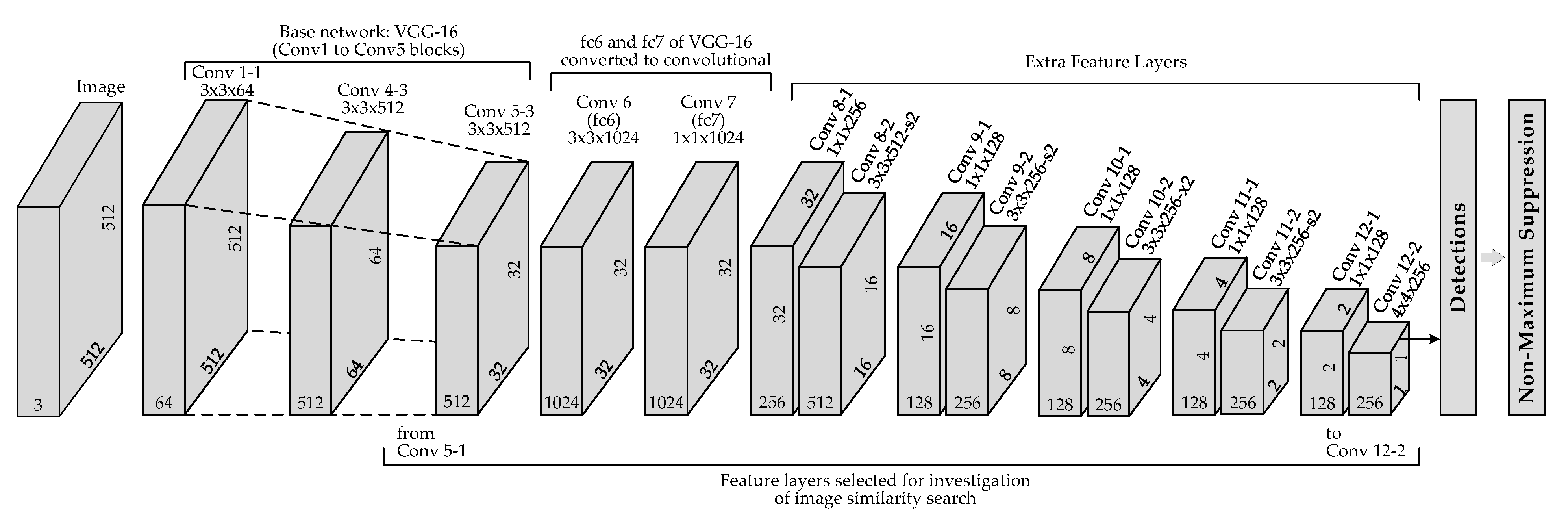
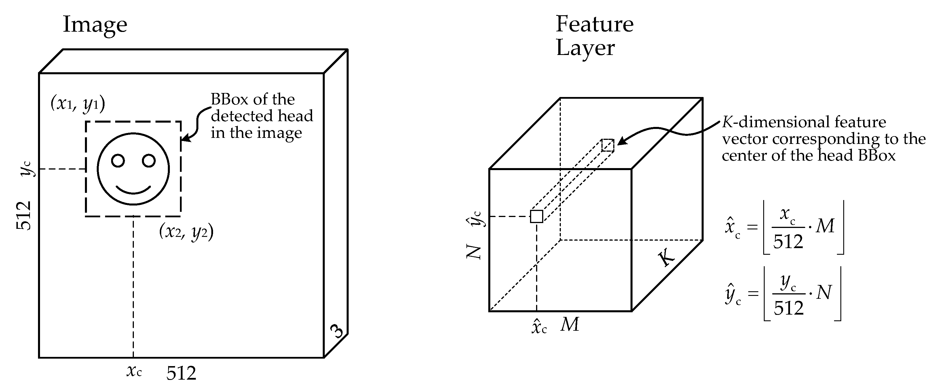
Table 1.
Summary of 3D reconstruction algorithms tested: baseline 3D reconstruction algorithm (1) and its variants (2a, 2b, 3a, 3b, 4a, 4b). All variants introduce head detection and discarding of feature points outside the bounding box of the head. Variants 3a, 3b, 4a, and 4b additionally utilize image quality during the frame number reduction but differ in the applied reduction strategy.
| Reconstruction Step 1 | Variant of 3D Reconstruction Pipeline | |||||||
|---|---|---|---|---|---|---|---|---|
| 1 | 2 | 3 | 4 | |||||
| (Baseline) | a | b | a | b | a | b | ||
| 1. | Load frames | + | + | + | + | |||
| 2. | Camera initialization | + | + | + | + | |||
| 3. | Head detection | – | + | + | + | |||
| 4. | Image quality estimation | – | – | + | + | |||
| 5. | Frame selection 2 | N-th | N-th | Best from N | Best from all | |||
| 6. | Feature point detection 3 (Normal–n; High–h) | n | n | h | n | h | n | h |
| 7. | Feature point selection (remove KPs outside BBox) | – | + | + | + | + | + | + |
| 8. | Feature description | + | + | + | + | + | + | + |
| 9. | Image matching | + | + | + | + | + | + | + |
| 10. | Feature (descriptor) matching | + | + | + | + | + | + | + |
| 11. | SfM (sparse reconstruction) | + | + | + | + | + | + | + |
1 reconstruction steps correspond to the order of the generalized 3D reconstruction pipeline in Figure 1; 2 frame selection strategies: “N-th”, selects every N-th frame; “Best from N”, selects the frame with the highest quality from consecutive N frames; “Best from all”, selects a certain number of frames from the full set of frames exploiting image quality and image similarity information; 3 Describer Density preset in Meshroom’s Feature Extraction node.
Table 2.
Summary of the CNN’s last 15 feature layers that were investigated for suitability to provide useful information for sorting images by similarity in order to predict the relative location of the frames in the space at the time of imaging.
Table 2.
Summary of the CNN’s last 15 feature layers that were investigated for suitability to provide useful information for sorting images by similarity in order to predict the relative location of the frames in the space at the time of imaging.
| Layer No. | Layer Name | Feature Layer Size | RF Size | |
|---|---|---|---|---|
| [] 1 | [px] 2 | [%] 3 | ||
| 11 | Conv 5-1 | 51 | 10 | |
| 12 | Conv 5-2 | 59 | 12 | |
| 13 | Conv 5-3 | 67 | 13 | |
| 14 | Conv 6 (fc6) | 287 | 56 | |
| 15 | Conv 7 (fc7) | 287 | 56 | |
| 16 | Conv 8-1 | 287 | 56 | |
| 17 | Conv 8-2 | 287 | 56 | |
| 18 | Conv 9-1 | 287 | 56 | |
| 19 | Conv 9-2 | 287 | 56 | |
| 20 | Conv 10-1 | 287 | 56 | |
| 21 | Conv 10-2 | 289 | 56 | |
| 22 | Conv 11-1 | 289 | 56 | |
| 23 | Conv 11-2 | 511 | 100 | |
| 24 | Conv 12-1 | 511 | 100 | |
| 25 | Conv 12-2 | 511 | 100 | |
1 (rows × columns × channels); 2 size of the layer unit’s receptive field in pixels; 3 size of the layer unit’s receptive field relative to the size of the input image, in percent.
Table 3.
Comparison of feature sources (convolutional layer number) and dimensionality-reduction techniques used to order images by similarity (closeness) in . The values in the table are scores (mean ± SD), which represent the number of correctly predicted images (in percent) being the most similar to the reference image. The best performance was highlighted in red.
| F 1 | D 2 | NoMap 3 | tSNE 4 | SNE 5 | MDS 6 | PCA 7 | ProbPCA 8 | KPCA 9 | LDA 10 | FA 11 | Sammon 12 | DM 13 | SPE 14 | GPLVM 15 | NCA 16 | LMNN 17 | 18 |
|---|---|---|---|---|---|---|---|---|---|---|---|---|---|---|---|---|---|
| 11 | 1 | ||||||||||||||||
| 2 | |||||||||||||||||
| 12 | 1 | ||||||||||||||||
| 2 | |||||||||||||||||
| 13 | 1 | ||||||||||||||||
| 2 | |||||||||||||||||
| 14 | 1 | ||||||||||||||||
| 2 | |||||||||||||||||
| 15 | 1 | ||||||||||||||||
| 2 | |||||||||||||||||
| 16 | 1 | ||||||||||||||||
| 2 | |||||||||||||||||
| 17 | 1 | ||||||||||||||||
| 2 | |||||||||||||||||
| 18 | 1 | ||||||||||||||||
| 2 | |||||||||||||||||
| 19 | 1 | ||||||||||||||||
| 2 | |||||||||||||||||
| 20 | 1 | ||||||||||||||||
| 2 | |||||||||||||||||
| 21 | 1 | ||||||||||||||||
| 2 | |||||||||||||||||
| 22 | 1 | ||||||||||||||||
| 2 | |||||||||||||||||
| 23 | 1 | ||||||||||||||||
| 2 | |||||||||||||||||
| 24 | 1 | ||||||||||||||||
| 2 | |||||||||||||||||
| 25 | 1 | ||||||||||||||||
| 2 | |||||||||||||||||
| 19 | 1 | ||||||||||||||||
| 2 |
1 feature layer number corresponding to the Table 2; 2 iteration of head detection in image; 3 evaluation results of image similarity without dimensionality reduction of the feature vector; dimensionality-reduction techniques: 4 t-Distributed Stochastic Neighbor Embedding (t-SNE), 5 Stochastic Neighbor Embedding (SNE), 6 Classical multidimensional scaling (MDS), 7 Principal Component Analysis (PCA), 8 Probabilistic PCA, 9 Kernel PCA, 10 Linear Discriminant Analysis (LDA), 11 Factor Analysis (FA), 12 Sammon mapping, 13 Diffusion maps, 14 Stochastic Proximity Embedding (SPE), 15 Gaussian Process Latent Variable Model (GPLVM), 16 Neighborhood Components Analysis (NCA), 17 Large-Margin Nearest Neighbor (LMNN); 18 score (mean ± SD) of all dimensionality-reduction techniques for different feature layers, 19 score (mean ± SD) of all feature layers for different dimensionality-reduction techniques.
Table 4.
Comparison of feature sources (convolutional layer number) and dimensionality-reduction techniques used to order images by similarity (closeness) in . The values in the table are scores (mean ± SD), which represent the number of correctly predicted images (in percent) being the most similar to the reference image. The best performance was highlighted in red.
| F 1 | D 2 | NoMap 3 | tSNE 4 | SNE 5 | MDS 6 | PCA 7 | ProbPCA 8 | KPCA 9 | LDA 10 | FA 11 | Sammon 12 | DM 13 | SPE 14 | GPLVM 15 | NCA 16 | LMNN 17 | 18 |
|---|---|---|---|---|---|---|---|---|---|---|---|---|---|---|---|---|---|
| 11 | 1 | ||||||||||||||||
| 2 | |||||||||||||||||
| 12 | 1 | ||||||||||||||||
| 2 | |||||||||||||||||
| 13 | 1 | ||||||||||||||||
| 2 | |||||||||||||||||
| 14 | 1 | ||||||||||||||||
| 2 | |||||||||||||||||
| 15 | 1 | ||||||||||||||||
| 2 | |||||||||||||||||
| 16 | 1 | ||||||||||||||||
| 2 | |||||||||||||||||
| 17 | 1 | ||||||||||||||||
| 2 | |||||||||||||||||
| 18 | 1 | ||||||||||||||||
| 2 | |||||||||||||||||
| 19 | 1 | ||||||||||||||||
| 2 | |||||||||||||||||
| 20 | 1 | ||||||||||||||||
| 2 | |||||||||||||||||
| 21 | 1 | ||||||||||||||||
| 2 | |||||||||||||||||
| 22 | 1 | ||||||||||||||||
| 2 | |||||||||||||||||
| 23 | 1 | ||||||||||||||||
| 2 | |||||||||||||||||
| 24 | 1 | ||||||||||||||||
| 2 | |||||||||||||||||
| 25 | 1 | ||||||||||||||||
| 2 | |||||||||||||||||
| 19 | 1 | ||||||||||||||||
| 2 |
1 feature layer number corresponding to the Table 2; 2 iteration of head detection in image; 3 evaluation results of image similarity without dimensionality reduction of the feature vector; dimensionality-reduction techniques: 4 t-Distributed Stochastic Neighbor Embedding (t-SNE), 5 Stochastic Neighbor Embedding (SNE), 6 Classical multidimensional scaling (MDS), 7 Principal Component Analysis (PCA), 8 Probabilistic PCA, 9 Kernel PCA, 10 Linear Discriminant Analysis (LDA), 11 Factor Analysis (FA), 12 Sammon mapping, 13 Diffusion maps, 14 Stochastic Proximity Embedding (SPE), 15 Gaussian Process Latent Variable Model (GPLVM), 16 Neighborhood Components Analysis (NCA), 17 Large-Margin Nearest Neighbor (LMNN); 18 score (mean ± SD) of all dimensionality-reduction techniques for different feature layers, 19 score (mean ± SD) of all feature layers for different dimensionality-reduction techniques.
Table 5.
Comparative results of 3D head reconstruction algorithms expressed as the residual errors (in arbitrary units, ×) of alignment of the test models to the reference model when the residuals are calculated in the full region of the head (Evaluation Case 1) and when the residuals are calculated only in the facial region of the head (Evaluation Case 2). The values in the table are the averages of reconstruction residuals ( confidence). The best result in each row is highlighted in red.
| Variant of 3D Reconstruction Pipeline 1 | |||||||
|---|---|---|---|---|---|---|---|
| Video | 1 (Baseline) | 2a | 2b | 3a | 3b | 4a | 4b |
| Evaluation case 1 (full region of the head) | |||||||
| 1 | |||||||
| 2 | |||||||
| 3 | |||||||
| 4 | |||||||
| 5 | |||||||
| 6 | |||||||
| 7 | |||||||
| 8 | |||||||
| 9 | |||||||
| 10 | n/a 2 | ||||||
| 11 | |||||||
| 12 | |||||||
| 13 | |||||||
| 14 | |||||||
| 15 | |||||||
| 16 | |||||||
| 17 | |||||||
| 18 | |||||||
| 19 | |||||||
| 3 | |||||||
| Evaluation case 2 (facial region of the head) | |||||||
| 1 | |||||||
| 2 | |||||||
| 3 | |||||||
| 4 | |||||||
| 5 | |||||||
| 6 | |||||||
| 7 | |||||||
| 8 | |||||||
| 9 | |||||||
| 10 | n/a 2 | ||||||
| 11 | |||||||
| 12 | |||||||
| 13 | |||||||
| 14 | |||||||
| 15 | |||||||
| 16 | |||||||
| 17 | |||||||
| 18 | |||||||
| 19 | |||||||
| 3 | |||||||
1 3D reconstruction algorithms are explained in Table 1; 2 head reconstruction did not provide a consistent model; 3 average of reconstruction residuals (±95% confidence) of all head models.
Table 6.
Descriptive statistics of experimental data.
| Variant of 3D Reconstruction Pipeline 1 | |||||||
|---|---|---|---|---|---|---|---|
| Attribute | 1 (Baseline) | 2a | 2b | 3a | 3b | 4a | 4b |
| Images2 | |||||||
| Image matches3 | |||||||
| Feature points4 | |||||||
| Points in PC15 | |||||||
| Points in PC26 | |||||||
1 3D reconstruction algorithms are explained in Table 1; 2 average number of frames (±SD) selected for the reconstruction; 3 average number of image matches (±SD) performed during reconstructions; 4 average number of feature points (±SD) extracted in images; 5, 6 average number of points (±SD) in point clouds of the full head and only in the face region, respectively.
Publisher’s Note: MDPI stays neutral with regard to jurisdictional claims in published maps and institutional affiliations. |
© 2021 by the authors. Licensee MDPI, Basel, Switzerland. This article is an open access article distributed under the terms and conditions of the Creative Commons Attribution (CC BY) license (https://creativecommons.org/licenses/by/4.0/).
Share and Cite
MDPI and ACS Style
Matuzevičius, D.; Serackis, A. Three-Dimensional Human Head Reconstruction Using Smartphone-Based Close-Range Video Photogrammetry. Appl. Sci. 2022, 12, 229. https://0-doi-org.brum.beds.ac.uk/10.3390/app12010229
AMA Style
Matuzevičius D, Serackis A. Three-Dimensional Human Head Reconstruction Using Smartphone-Based Close-Range Video Photogrammetry. Applied Sciences. 2022; 12(1):229. https://0-doi-org.brum.beds.ac.uk/10.3390/app12010229
Chicago/Turabian StyleMatuzevičius, Dalius, and Artūras Serackis. 2022. "Three-Dimensional Human Head Reconstruction Using Smartphone-Based Close-Range Video Photogrammetry" Applied Sciences 12, no. 1: 229. https://0-doi-org.brum.beds.ac.uk/10.3390/app12010229
Note that from the first issue of 2016, this journal uses article numbers instead of page numbers. See further details here.