Undrained Elastoplastic Solution for Cylindrical Cavity Expansion in Structured Cam Clay Soil Considering the Destructuration Effects

Abstract

Soil structure has significant influences on the mechanical behaviors of natural soils, although it is rarely considered in previous cavity expansion analyses. This paper presents an undrained elastoplastic solution for cylindrical cavity expansion in structured soils, considering the destructuration effects. Firstly, a structural ratio was defined to denote the degree of the initial structure, and the Structured Cam Clay (SCC) model was employed to describe the subsequent stress-induced destructuration, including the structure degradation and crushing. Secondly, combined with the large strain theory, the considered problem was formulated as a system of first-order differential equations, which can be solved in a simplified procedure with the introduced auxiliary variable. Finally, the significance and efficiency of the present solution was demonstrated by comparing with the previous solutions, and parametric studies were also conducted to investigate the effects of soil structure and destructuration on the cavity expansion process. The results show that the soil structure has pronounced effects on the mechanical behavior of structured soils around the cavity. For structured soils, a cavity pressure that is larger than the corresponding reconstituted soils when the cavity expands to the same radius is required, and the effective stresses first increase to a peak value before decreasing rapidly with soil structure degradation and crushing. The same final critical state is reached for soils with different degrees of the initial structure, which indicates that the soil structure is completely destroyed during the cavity expansion. With the increase of the destructuring index, the soil structure was destroyed more rapidly, and the stress release during the plastic deformation became more significant. Moreover, the present solution was applied in the jacking of a casing during the sand compact pile installation and in situ self-boring pressuremeter (SBPM) tests, which indicates that the present solution provides an effective theoretical tool for predicting the behavior of natural structured soils around the cavity.

1. Introduction

Cavity expansion theory provides a useful, accurate, and simple tool for modelling many complex geotechnical problems [1], such as the interpretation of the results of pressuremeter and cone penetration tests [2,3,4], the estimation of stress responses around installed piles [5,6,7], as well as the stability and deformation analyses for wellbore drilling and tunnel excavation [8,9,10,11]. Therefore, it has received wide attention and made great progress over the past few decades.

In previous studies, a variety of constitutive models were employed to develop analytical/semi-analytical cavity expansion solutions [12]. The early solutions were mostly based on the Mohr–Coulomb criterion [2,13,14] and the Drucker–Prager criterion [15], in which the soil was assumed to be the elastic–perfectly plastic materials. Consequently, the influences of stress history and strain hardening/softening on the mechanical behavior of soils around the cavity could not be considered in these solutions [16]. With the development of constitutive models, critical state soil models were introduced into the cavity expansion analyses. For example, Collins and Stimpson [17] proposed the similarity technique based on the Modified Cam Clay (MCC) model for the undrained and drained cavity expansion problems. Later, this solution technique was extended into the bounding surface model [18,19], the clay and soil model (CASM) [10,20], the thermoplastic soil model [21], and so on. Because the deviator mean effective stresses were simplified in the above similarity technique, Chen and Abousleiman [22,23] proposed an exact solution technique for the cavity expansion in MCC soil, following their rigorous definitions. In this framework, many researchers have developed a series of cavity expansion solutions by employing various constitutive models, such as the anisotropic soil model [12,24,25] and unsaturated soil model [26,27]. However, the above-mentioned solutions are suitable for modelling the behavior of reconstituted soils rather than natural structured soils around the cavity because the soil structure was not taken into account. The structure, as one of the most significant features influencing the mechanical behaviors of naturally deposited soils [28], is rarely accounted for in previous cavity expansion analyses.

More than a decade ago, several attempts were made to explore the cavity expansion responses in structured soils using a relatively simple constitutive model [29,30]. Recently, Sivasithamparam and Castro [31] extended their anisotropic solution [25] by incorporating the effects of structure on the soil behavior by updating the employed constitutive model from the S-CLAY1 [32] to the S-CLAY1S model [33]. This solution is at the cost of complexity, though the better results can be obtained. For this reason, Li et al. [34] presented a drained solution for structured soils considering structure degradation, based on the Structured Cam Clay (SCC) model proposed by Liu and Carter [35]. Actually, the pile installation, standard pressuremeter, and cone penetration tests in clay usually involve an undrained process; the undrained cavity expansion solution, as a theoretical tool to model these engineering problems, is more urgently needed than the drained one. Therefore, an undrained solution was also proposed by Li et al. [36], in which the Modified Cam Clay model of structured loess was adopted. However, in their solution [34,36], only the initial soil structure was considered; the structure could not be completely removed even though the ultimate critical state was reached, which resulted in an inability to capture the softening behavior of structured.

In this study, an undrained elastoplastic solution for cylindrical cavity expansion in structured soils is proposed. The destructuration effects, including the structure degradation and crushing, are considered by employing the SCC model of Carter and Liu [37], in which the complete removal of the soil structure can be achieved. By introducing an auxiliary variable, the mechanical behavior of structured soils around the cavity is governed by a system of differential equations, though the flow rules in the SCC model follow different forms during the hardening, softening, and crushing processes. The significance and efficiency of the present solution was demonstrated by comparing them with the previous solutions. Subsequently, the parametric studies were conducted to investigate the effects of soil structure and destructuration on the cavity expansion process. Finally, the jacking of a casing during the sand compact pile installation and in situ self-boring pressuremeter (SBPM) tests were analyzed to illustrate the applicability of the present solution.

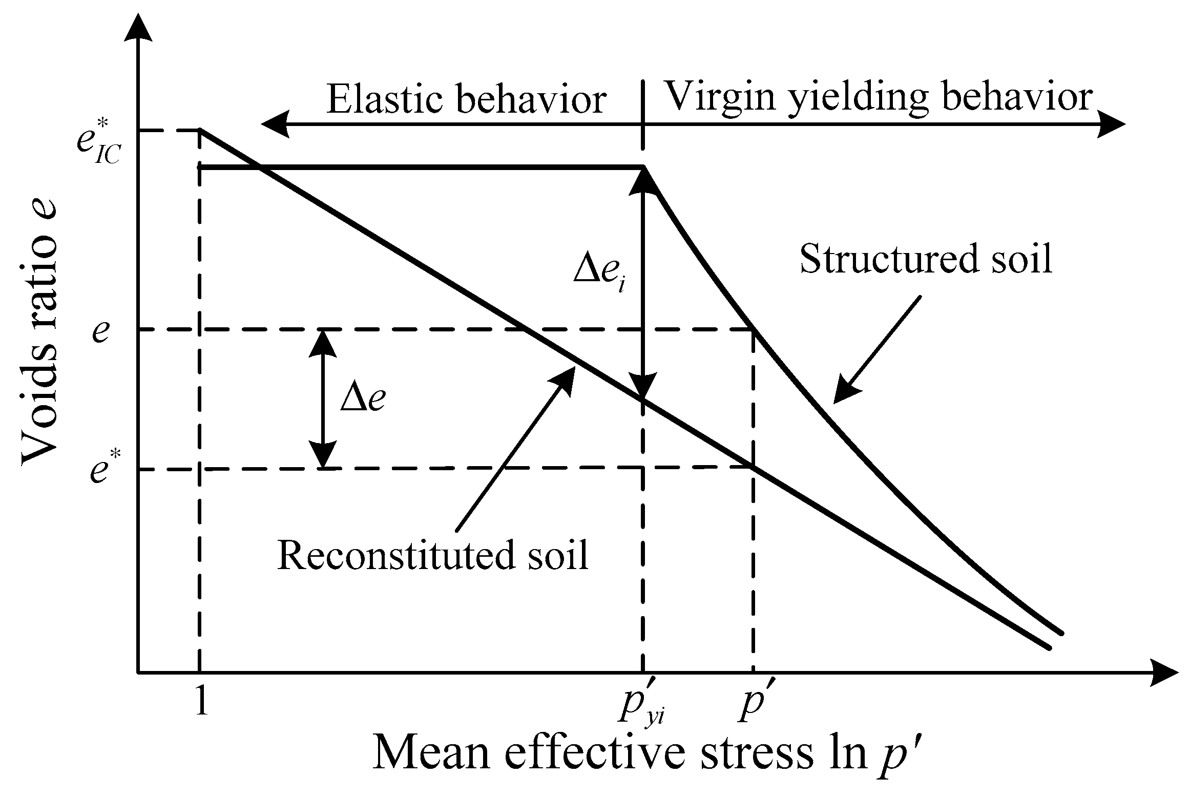
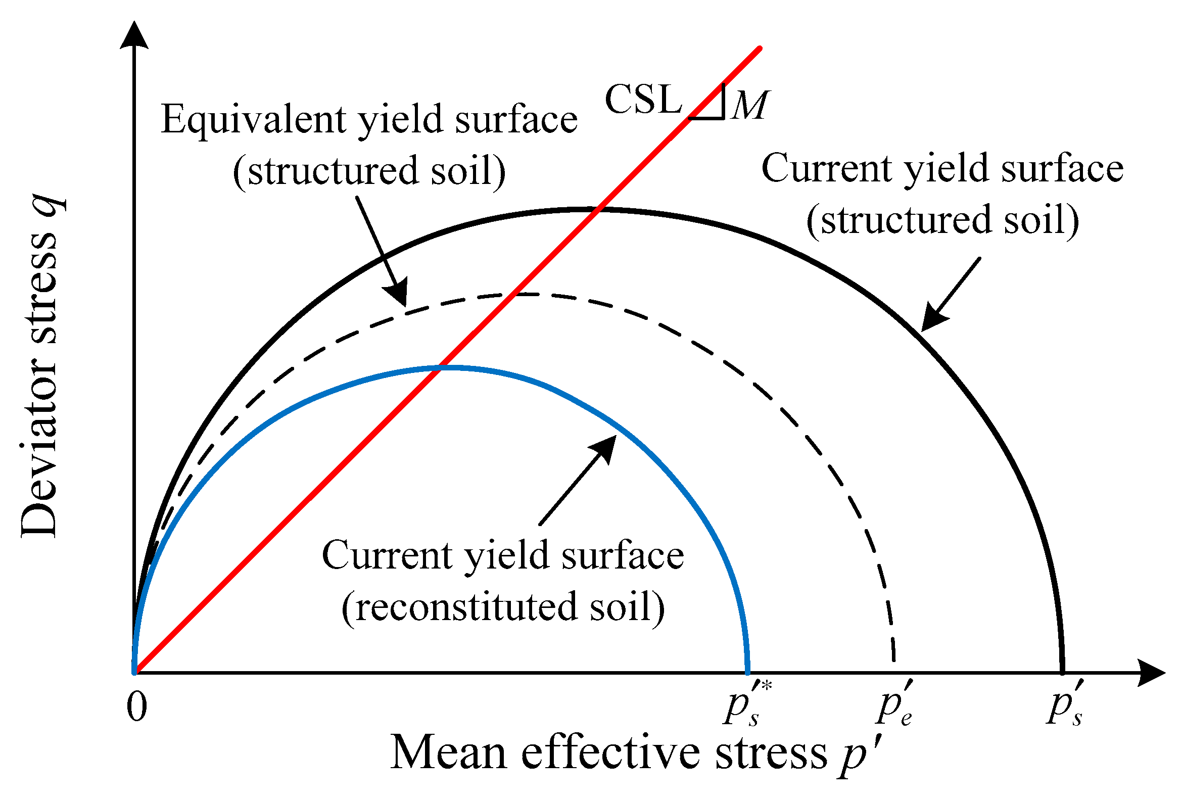
2. Structured Cam Clay Model

The SCC model [37] involves only a few conveniently identified parameters; however, it is still capable of capturing the destructuration of natural soils, including the structure degradation and crushing [38]. According to the fact that the voids ratio of naturally structured soils e is larger than that of the corresponding reconstituted soils e* at the same stress state [39], the isotropic compression behavior of structured soils in the SCC model is idealized, as shown in Figure 1, and the decrease of Δe (the difference between e and e*) represents the destructuration of soils. For isotropic compression virgin yield (p′ > p′_yi), the additional voids ratio Δe of structured soils can be given by [37]

$$\Delta e=\left(\Delta e_i-c\right){\left(\frac{p_{yi}^{\prime }}{p^{\prime }}\right)}^b+c$$

(1)

where p′ is the current mean effective stress, p′_yi is the initial yield stress of structured soils under isotropic compression, and b is the isotropic compression destructuring index. Δe_i is the value of Δe at p′ = p′_yi, and c is a stable value of Δe when p′ is sufficiently large.

As a Cam Clay model, it is assumed that the yield surface of structured soils in the p′–q plane is elliptical, as shown in Figure 2, which is larger than that of the corresponding reconstituted soils, and can be formulated as [37]

$$f=q^2-M^2{p}^{\prime }\left(p_s^{\prime }-p^{\prime }\right)=0$$

(2)

where M, named the critical state stress ratio, represents the slope of the critical state line (CSL), q is the deviator stress that follows its standard three-dimensional definition in this study, and p′_s is the isotropic yield stress denoting the size of the yield surface.

The initial yield surface of structured soils enlarges with the increase of structure, as shown in Figure 2. The equivalent yield surface for structured soils, i.e., the dashed line in Figure 2, is defined as a yield surface for the soils remolded with the same voids ratio and stress state [37]. The size of the equivalent yield surface is denoted by p′_e, whose value can be determined by the states (p′ and e) of structured soils, as follows:

$$p_e^{\prime }=\exp \left(\frac{e_{IC}^{\ast }-e-\kappa \ln p^{\prime }}{\lambda -\kappa }\right)$$

(3)

where $e_{IC}^{\ast }$ is the voids ratio for reconstituted soils when p′ = 1 kPa, as shown in Figure 1. λ and κ denote the slopes of the compression and loading–reloading lines of the reconstituted soils, respectively.

When the stress state reaches the structural yield surface with dp′_s ≠ 0, virgin yielding occurs and is accompanied by the destructuration, which is an irreversible process. Considering the contribution of shearing on the destructuration of soils, the plastic volumetric strain increment can be described as

$$d{\epsilon }_v^p=\left[\lambda -\kappa +b\left(\langle \Delta e-c\rangle +\frac{\gamma \eta \Delta e}{M-\eta }\right)\right]\frac{d{p}_s^{\prime }}{\left(1+e\right)p_s^{\prime }}$$

(4)

where η = q/p′ is the stress ratio, γ is the shearing destructuring index, and < > is the Macaulay bracket.

Additionally, it was observed that the flow rule, the strain increment ratio ${d\epsilon }_d^p$/${d\epsilon }_v^p$, is also significantly affected by the soil structure [40]. The non-associated flow rules, defining the yield surface as inconsistent with the plastic potential surface, are employed in the SCC model to incorporate the influences of structure. For virgin yielding with η < M, hardening occurs, and the flow rule is given by

$$\frac{d{\epsilon }_d^p}{d{\epsilon }_v^p}=\frac{2\eta }{\left|M^2-{\eta }^2\right|+\omega {\eta }^2\left|1-\sqrt{p_e^{\prime }/p_s^{\prime }}\right|}={\beta }_1$$

(5)

where ω is a material constant describing the flow rule. As suggested by Carter and Liu [37], the value of ω is normally set to 1 when the experimental data is insufficient.

For virgin yielding with η > M, softening occurs. During this process, the yield surface shrinks with the destructuration of soils. As a result, it is necessary to change the sign of the plastic deviatoric strain associated with destructuration to ensure the strain increment direction is always outwards of the structured yield surface [35,37]. In this situation, the flow rule can be expressed as

$$\frac{d{\epsilon }_d^p}{d{\epsilon }_v^p}=-{\beta }_1\frac{\lambda -\kappa +b\left(\langle \Delta e-c\rangle -\frac{\gamma \eta \Delta e}{M-\eta }\right)}{\lambda -\kappa +b\left(\langle \Delta e-c\rangle +\frac{\gamma \eta \Delta e}{M-\eta }\right)}={\beta }_2$$

(6)

Structured soils that undergo virgin yielding may reach a critical state (η = M), but the structure is not completely destroyed (Δe ≠ 0), which means that the plastic deformation will develop continuously with the further loading [38]. This stage is termed the crushing of soil structure and was first introduced into the SCC model by Carter and Liu [37]. During the structure crushing, the stress state always varies along the CSL, which follows

$$dq=Md{p}^{\prime }$$

(7)

Meanwhile, the additional voids ratio Δe gradually diminishes with the structure crushing, and tends to be c when the stress state reaches a final critical state. During this process, the flow rule is given by

$$\frac{d{\epsilon }_d^p}{d{\epsilon }_v^p}=\frac{2\mathrm{sign}(d{\epsilon }_v^p)}{\omega \eta \left|1-\sqrt{p_e^{\prime }/p_s^{\prime }}\right|}={\beta }_3$$

(8)

where sign( ) denotes the signum function.

3. Cylindrical Cavity Expansion in the SCC Soil

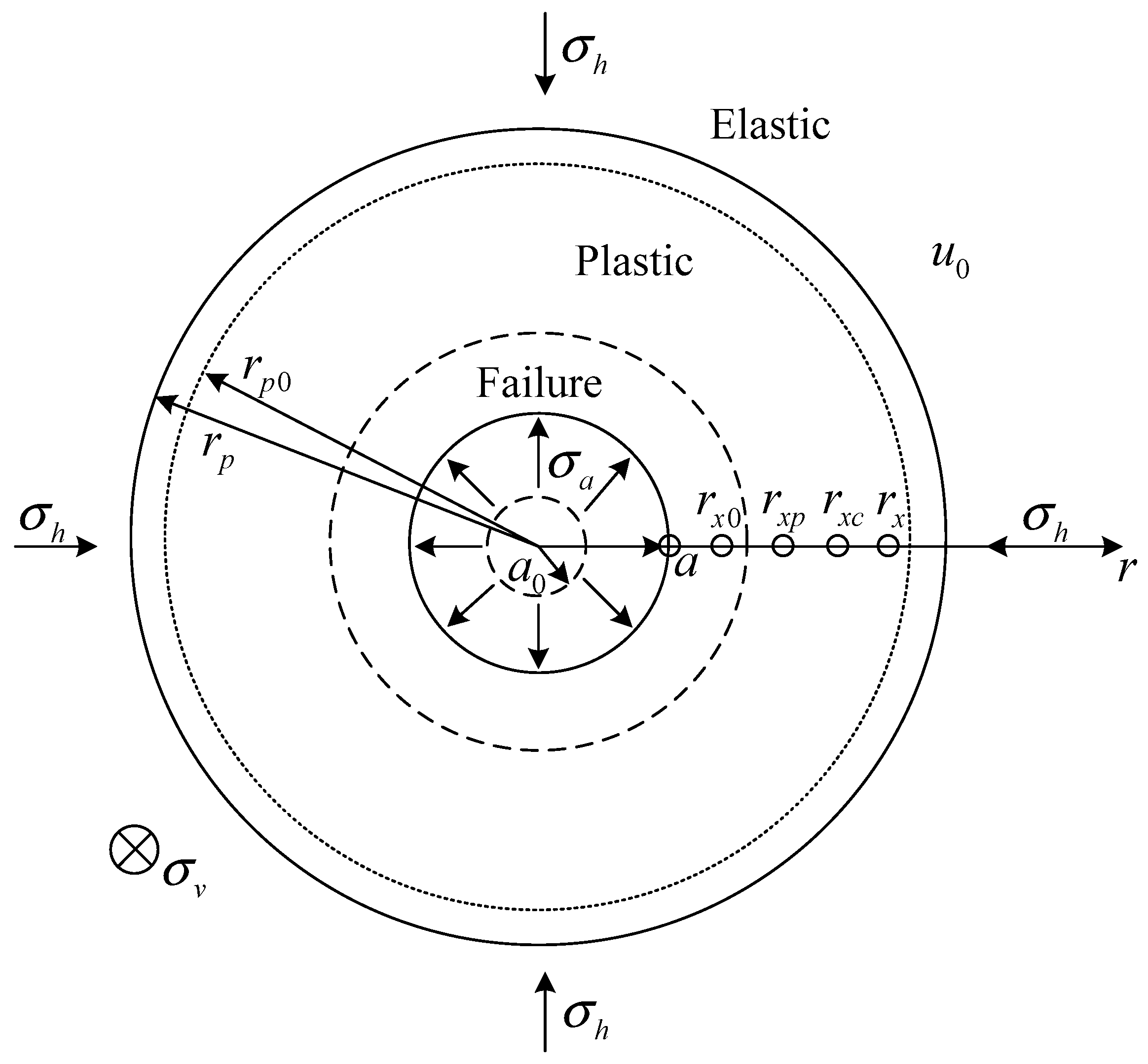
3.1. Problem Description

The undrained expansion of a cylindrical cavity with an initial radius a₀ in an infinite structured soil is schematically shown in Figure 3, where σ_h and σ_v denote the initial horizontal and vertical total stress, respectively, and u₀ is the initial pore pressure. As the internal pressure σ_a increases gradually from its initial value σ_h, the cavity expands from a₀ to a larger cavity radius a. Meanwhile, a typical soil element moves outward along the radial direction from the initial position r_x0 to the current position r_x. During this process, the soil element first undergoes elastic deformation until the initial yielding occurs, and then experiences plastic hardening or softening with structure degradation. The soil structure begins to be crushed if the soil element with an incompletly destroyed structure may attain a critical state before reaching the current position, r_x. In Figure 3, r_xp and r_xc denote the positions of the soil element at the precise moment when it enters the plastic state and when its structure begins to be crushed.

Cylindrical coordinates (r, θ, z) are considered because of the symmetry of the cylindrical cavity expansion problem. Considering a soil element located at the radial position r with unit height in z direction, the radial and tangential total stresses, σ_r and σ_θ, satisfy the force equilibrium equation as follows:

$$\frac{d{\sigma }_r}{dr}+\frac{{\sigma }_r-{\sigma }_{\theta }}{r}=0$$

(9)

According to the Terzaghi effective stress principle, Equation (9) can be written as

$$\frac{d{\sigma }_r^{\prime }}{dr}+\frac{du}{dr}+\frac{{\sigma }_r^{\prime }-{\sigma }_{\theta }^{\prime }}{r}=0$$

(10)

where σ′_r and σ′_θ are the effective components corresponding to σ_r and σ_θ, respectively, and u is the pore pressure at position r.

3.2. Elastic Analysis

The structured soils undergo elastic deformation before the stress state reaches the initial yield surface. The elastic stress–strain relationship obeys Hooke’s law, and can be written in the following incremental form

$$d{\epsilon }_{ij}^e=\frac{1+v}{E}d{\sigma }_{ij}^{\prime }-\frac{v}{E}d{\sigma }_{mm}^{\prime }{\delta }_{ij}$$

(11)

where E is the Young’s modulus, v is the effective Poisson’s ratio, and δ_ij is the Kronecker delta.

In the SCC model, v is treated as a constant, and E can be expressed in terms of v and shear modulus G, namely E = 2G(1 + v), where G is related to the mean effective stress p′ and the voids ratio e is

$$G=\frac{3\left(1-2v\right)\left(1+e\right)p^{\prime }}{2(1+v)\kappa }$$

(12)

Combining the elastic stress–strain relationship (Equation (11)) and the effective equilibrium equation (Equation (10)), three effective stress components, σ′_r, σ′_θ, σ′_z, the radial displacement U_r, and the pore pressure u can be explicitly expressed as [1,22]:

$${\sigma }_r^{\prime }={\sigma }_h^{\prime }+({\sigma }_{rp}^{\prime }-{\sigma }_h^{\prime }){\left(\frac{r_p}{r}\right)}^2$$

(13)

$${\sigma }_{\theta }^{\prime }={\sigma }_h^{\prime }-({\sigma }_{rp}^{\prime }-{\sigma }_h^{\prime }){\left(\frac{r_p}{r}\right)}^2$$

(14)

$${\sigma }_z^{\prime }={\sigma }_v^{\prime }$$

(15)

$$U_r=\frac{{\sigma }_{rp}^{\prime }-{\sigma }_h^{\prime }}{2G}\frac{r_p^2}{r}$$

(16)

$$u=u_0$$

(17)

where σ′_rp is the specific value of σ′_r at the elastoplastic boundary r_p.

3.3. Elastoplastic Analysis

For the natural soils, the plastic deformation is usually accompanied by the elastic deformation; therefore, the components of the total strain increment dε_i consists of the elastic strain increment ${d\epsilon }_i^e$ and plastic strain increment ${d\epsilon }_i^p$, i.e.,

$$d{\epsilon }_i=d{\epsilon }_i^e+d{\epsilon }_i^{p}i=r,\theta ,z$$

(18)

where ${d\epsilon }_i^e$ can be calculated using Equation (11), and ${d\epsilon }_i^p$ is controlled by the yield function, the hardening (or softening) law, and the plastic flow rules of the SCC model.

In order to derive the components of plastic strain increment ${d\epsilon }_i^p$, the consistency condition, i.e., df = 0, is applied to the yield function in Equation (2), and yields

$$df={\left\{\frac{\partial f}{\partial {\sigma }_i^{\prime }}\right\}}^T\left\{d{\sigma }_i^{\prime }\right\}+\frac{\partial f}{\partial p_s^{\prime }}\frac{\partial p_s^{\prime }}{\partial {\epsilon }_v^p}d{\epsilon }_v^p=0$$

(19)

where

$${\left\{\frac{\partial f}{\partial {\sigma }_i^{\prime }}\right\}}^T=\left[\begin{array}{ccc}\frac{\partial f}{\partial {\sigma }_r^{\prime }}& \frac{\partial f}{\partial {\sigma }_{\theta }^{\prime }}& \frac{\partial f}{\partial {\sigma }_z^{\prime }}\end{array}\right]$$

(20)

$$\left\{d{\sigma }_i^{\prime }\right\}={\left[\begin{array}{ccc}d{\sigma }_r^{\prime }& d{\sigma }_{\theta }^{\prime }& d{\sigma }_z^{\prime }\end{array}\right]}^T$$

(21)

Therefore, the plastic volumetric strain increment ${d\epsilon }_v^p$ is given as

$$d{\epsilon }_v^p=\frac{{\left\{\frac{\partial f}{\partial {\sigma }_i^{\prime }}\right\}}^T\left\{d{\sigma }_i^{\prime }\right\}}{-\frac{\partial f}{\partial p_s^{\prime }}\frac{\partial p_s^{\prime }}{\partial {\epsilon }_v^p}}=\frac{1}{K_p}{\left\{\frac{\partial f}{\partial {\sigma }_i^{\prime }}\right\}}^T\left\{d{\sigma }_i^{\prime }\right\}=\mathsf{\Lambda }\frac{\partial g}{\partial p^{\prime }}$$

(22)

where g denotes the plastic potential function, Λ is the plastic multiplier, and

$$K_p=-\frac{\partial f}{\partial p_s^{\prime }}\frac{\partial p_s^{\prime }}{\partial {\epsilon }_v^p}$$

(23)

During the hardening (η < M) and softening (η > M) processes, the plastic volumetric strain can be described using Equation (4), and yields

$$\frac{\partial p_s^{\prime }}{\partial {\epsilon }_v^p}=\frac{\left(1+e\right)p^{\prime }}{\lambda -\kappa +b\left(\langle \Delta e-c\rangle +\frac{\gamma \eta \Delta e}{M-\eta }\right)}$$

(24)

During the crushing process (η = M), the effective stress states satisfy Equation (7). Therefore,

$$\frac{\partial p_s^{\prime }}{\partial {\epsilon }_v^p}=\frac{\partial p_s^{\prime }}{\partial p^{\prime }}\frac{\partial p^{\prime }}{\partial {\epsilon }_v^p}+\frac{\partial p_s^{\prime }}{\partial q}\frac{\partial q}{\partial {\epsilon }_v^p}=\left(\frac{\partial p_s^{\prime }}{\partial p^{\prime }}+M\frac{\partial p_s^{\prime }}{\partial q}\right)\frac{\partial p^{\prime }}{\partial {\epsilon }_v^p}$$

(25)

The total volumetric strain increment dε_v is zero under the undrained condition, which leads to the elastic strain and plastic strain, which can be compensated for each other, namely, ${d\epsilon }_p^v=-{d\epsilon }_v^e$. According to Equation (11), the term ∂p′/${\partial \epsilon }_v^p$ in Equation (25) can be obtained as follows:

$$\frac{\partial p^{\prime }}{\partial {\epsilon }_v^p}=-\frac{\left(1+e\right)p^{\prime }}{\kappa }$$

(26)

By combining Equation (22) and the non-associated flow rules Equations (5), (6), or (8), the plastic deviator strain increment ${d\epsilon }_d^p$ can be expressed in the following unified form:

$$d{\epsilon }_d^p=\frac{\beta }{K_p}{\left\{\frac{\partial f}{\partial {\sigma }_i^{\prime }}\right\}}^T\left\{d{\sigma }_i^{\prime }\right\}=\mathsf{\Lambda }\frac{\partial g}{\partial q}$$

(27)

where $\beta ={\partial \epsilon }_d^p/{\partial \epsilon }_v^p$ represents the plastic flow rule, which follows the different forms in the processes of hardening (β = β₁), softening (β = β₂), and crushing (β = β₃).

Combining Equations (22) and (27), the components of the plastic strain increments can be obtained as follows:

$$\begin{array}{cc}\begin{array}{cc}d{\epsilon }_i^p& =\mathsf{\Lambda }\frac{\partial g}{\partial {\sigma }_i^{\prime }}=\mathsf{\Lambda }\frac{\partial g}{\partial p^{\prime }}\frac{\partial p^{\prime }}{\partial {\sigma }_i^{\prime }}+\mathsf{\Lambda }\frac{\partial g}{\partial q}\frac{\partial q}{\partial {\sigma }_i^{\prime }}\hfill \\ & =\frac{1}{K_p}\left\{\frac{\partial p^{\prime }}{\partial {\sigma }_i^{\prime }}+\beta \frac{\partial q}{\partial {\sigma }_i^{\prime }}\right\}{\left\{\frac{\partial f}{\partial {\sigma }_j^{\prime }}\right\}}^T\left\{d{\sigma }_j^{\prime }\right\}\hfill \end{array}& i,j=r,\theta ,z\end{array}$$

(28)

Rewriting Equation (28) in matrix form, the following can be obtained:

$$\left\{\begin{array}{c}d{\epsilon }_r^p\\ d{\epsilon }_{\theta }^p\\ d{\epsilon }_z^p\end{array}\right\}=\frac{1}{K_p}\left[\begin{array}{ccc}{A}_r{B}_r& A_r{B}_{\theta }& A_r{B}_z\\ A_{\theta }{B}_r& A_{\theta }{B}_{\theta }& A_{\theta }{B}_z\\ A_z{B}_r& A_z{B}_{\theta }& A_z{B}_z\end{array}\right]\left\{\begin{array}{c}d{\sigma }_r^{\prime }\\ d{\sigma }_{\theta }^{\prime }\\ d{\sigma }_z^{\prime }\end{array}\right\}$$

(29)

where

$$A_i=\frac{\partial p^{\prime }}{\partial {\sigma }_i^{\prime }}+\beta \frac{\partial q}{\partial {\sigma }_i^{\prime }}=\frac{1}{3}+\frac{3\beta \left({\sigma }_i^{\prime }-p^{\prime }\right)}{2q}$$

(30)

$$B_j=\frac{\partial f}{\partial {\sigma }_j^{\prime }}=\frac{p^{\prime }\left(M^2-{\eta }^2\right)}{3}+3\left({\sigma }_i^{\prime }-p^{\prime }\right)$$

(31)

Substituting Equations (11) and (29) into Equation (18), the relationship between total strain components and effective stress components can be expressed as follows:

$$\left\{\begin{array}{c}d{\epsilon }_r\\ d{\epsilon }_{\theta }\\ d{\epsilon }_z\end{array}\right\}=\left[\begin{array}{ccc}\frac{A_r{B}_r}{K_p}+\frac{1}{E}& \frac{A_r{B}_{\theta }}{K_p}-\frac{v}{E}& \frac{A_r{B}_z}{K_p}-\frac{v}{E}\\ \frac{A_{\theta }{B}_r}{K_p}-\frac{v}{E}& \frac{A_{\theta }{B}_{\theta }}{K_p}+\frac{1}{E}& \frac{A_{\theta }{B}_z}{K_p}-\frac{v}{E}\\ \frac{A_z{B}_r}{K_p}-\frac{v}{E}& \frac{A_z{B}_{\theta }}{K_p}-\frac{v}{E}& \frac{A_z{B}_z}{K_p}+\frac{1}{E}\end{array}\right]\left\{\begin{array}{c}d{\sigma }_r^{\prime }\\ d{\sigma }_{\theta }^{\prime }\\ d{\sigma }_z^{\prime }\end{array}\right\}$$

(32)

By taking the inverse form of Equation (32), the components of stress increment can be expressed in terms of the components of strain increment as

$$\left\{\begin{array}{c}d{\sigma }_r^{\prime }\\ d{\sigma }_{\theta }^{\prime }\\ d{\sigma }_z^{\prime }\end{array}\right\}=\frac{1}{\Gamma }\left[\begin{array}{ccc}{C}_{rr}& C_{r\theta }& C_{rz}\\ C_{\theta r}& C_{\theta \theta }& C_{\theta z}\\ C_{zr}& C_{z\theta }& C_{zz}\end{array}\right]\left\{\begin{array}{c}d{\epsilon }_r\\ d{\epsilon }_{\theta }\\ d{\epsilon }_z\end{array}\right\}$$

(33)

where

$$C_{ii}=E\left[K_p(1-v^2)+E(A_j{B}_j+A_k{B}_k)+Ev(A_j{B}_k+A_k{B}_j)\right]i,j,k=r,\theta ,Z;i\ne j\ne k$$

(34a)

$$C_{ij}=E\left[K_p(v+v^2)-E{A}_i{B}_j-Ev(A_i{B}_k+A_k{B}_j-A_k{B}_k)\right]i,j,k=r,\theta ,z;i\ne j\ne k$$

(34b)

$$\Gamma =(v+1)\left[\begin{array}{l}{K}_p(1-v-2v^2)+E(1-v)(A_r{B}_r+A_{\theta }{B}_{\theta }+A_z{B}_z)\\ +Ev(A_r{B}_{\theta }+A_{\theta }{B}_r+A_{\theta }{B}_z+A_z{B}_{\theta }+A_r{B}_z+A_z{B}_r)\end{array}\right]i,j,k=r,\theta ,z;i\ne j\ne k$$

(34c)

Under the undrained and plane-strain assumptions, the volumetric strain increment dε_v and vertical strain increment dε_z are zero, which leads to dε_r = −dε_θ, and therefore Equation (33) becomes

$$d{\sigma }_r^{\prime }=\frac{-C_{rr}+C_{r\theta }}{\Gamma }d{\epsilon }_{\theta }$$

(35a)

$$d{\sigma }_{\theta }^{\prime }=\frac{-C_{\theta r}+C_{\theta \theta }}{\Gamma }d{\epsilon }_{\theta }$$

(35b)

$$d{\sigma }_z^{\prime }=\frac{-C_{zr}+C_{z\theta }}{\Gamma }d{\epsilon }_{\theta }$$

(35c)

According to the large strain theory, the tangential strain increment dε_θ in Equation (35a–c) can be expressed in the logarithmic strain form as

$$d{\epsilon }_{\theta }=-\frac{dr}{r}$$

(36)

Substituting Equation (36) into Equation (35a–c), it can be seen that three stress components, σ′_r, σ′_θ, and σ′_z, are functions of radial distance r. Note that the expressions of C_ij and Γ in Equation (35a–c) is inconsistent in the hardening/softening and crushing processes. For the hardening/softening process of the structured soils, the variations of the stress components can be calculated by taking the values of σ′_r(r_xp), σ′_θ(r_xp), and σ′_z(r_xp) as the initial values. If the soil element attains the critical state but with Δe ≠ c, the crushing of the structure will occur at a subsequent stage, which needs to be further solved by taking the values of σ′_r(r_xc), σʹ_θ(r_xc), and σ′_z(r_xc) as the initial values. However, it is complex to determine r_xc because it depends not only on the current radial location r, but also on the nonlinear displacement U_r during the hardening/softening process.

To simplify the solution procedure, the auxiliary variable ξ, defined by Chen and Abousleiman [23] as U_r/r, is skillfully introduced, where U_r = r − r₀ is the radial displacement for a specific soil element. This auxiliary variable takes the incremental form as follows:

$$\frac{d\xi }{1-\xi }=\frac{dr}{r}$$

(37)

Combining Equations (36) and (37), it can be seen that the tangential strain increment dε_θ is merely related to ξ; therefore, Equation (35a–c) can be written as

$$\frac{d{\sigma }_r^{\prime }}{d\xi }=\frac{C_{rr}-C_{r\theta }}{\Gamma (1-\xi )}$$

(38a)

$$\frac{d{\sigma }_{\theta }^{\prime }}{d\xi }=\frac{C_{\theta r}-C_{\theta \theta }}{\Gamma (1-\xi )}$$

(38b)

$$\frac{d{\sigma }_z^{\prime }}{d\xi }=\frac{C_{zr}-C_{z\theta }}{\Gamma (1-\xi )}$$

(38c)

Equation (38a–c) formulate the problem as a system of first-order differential equations with respect to a single variable ξ, which are valid for any soil element around the cavity. The values of σ′_r, σ′_θ, and σ′_z at the instant of ξ = ξ_p and ξ = ξ_c are required as the initial values of the hardening/softening and crushing processes, where ξ_p and ξ_c correspond to the values of u_r/r at the positions r_xp and r_xc, respectively. The values of σ′_r(ξ_c), σ′_θ(ξ_c), and σ′_z(ξ_c) as the initial values of the crushing process can be determined from the hardening/softening process, owing to the continuity of deformation; therefore, the values of σ′_r(ξ_p), σ′_θ(ξ_p), and σ′_z(ξ_p) are sufficient to solve the stress variation for a specific soil element. Meanwhile, because the cavity expansion is geometrically self-similar, the soil elements at any position r follow the same stress path [41]. Consequently, only the stress variation of the soil element at the cavity wall that undergoes the longest stress path needs to be calculated. For other soil elements around the cavity, the stress state only depends on ξ, which can be found from the experienced stress state of the soil element at the cavity wall by seeking the same ξ.

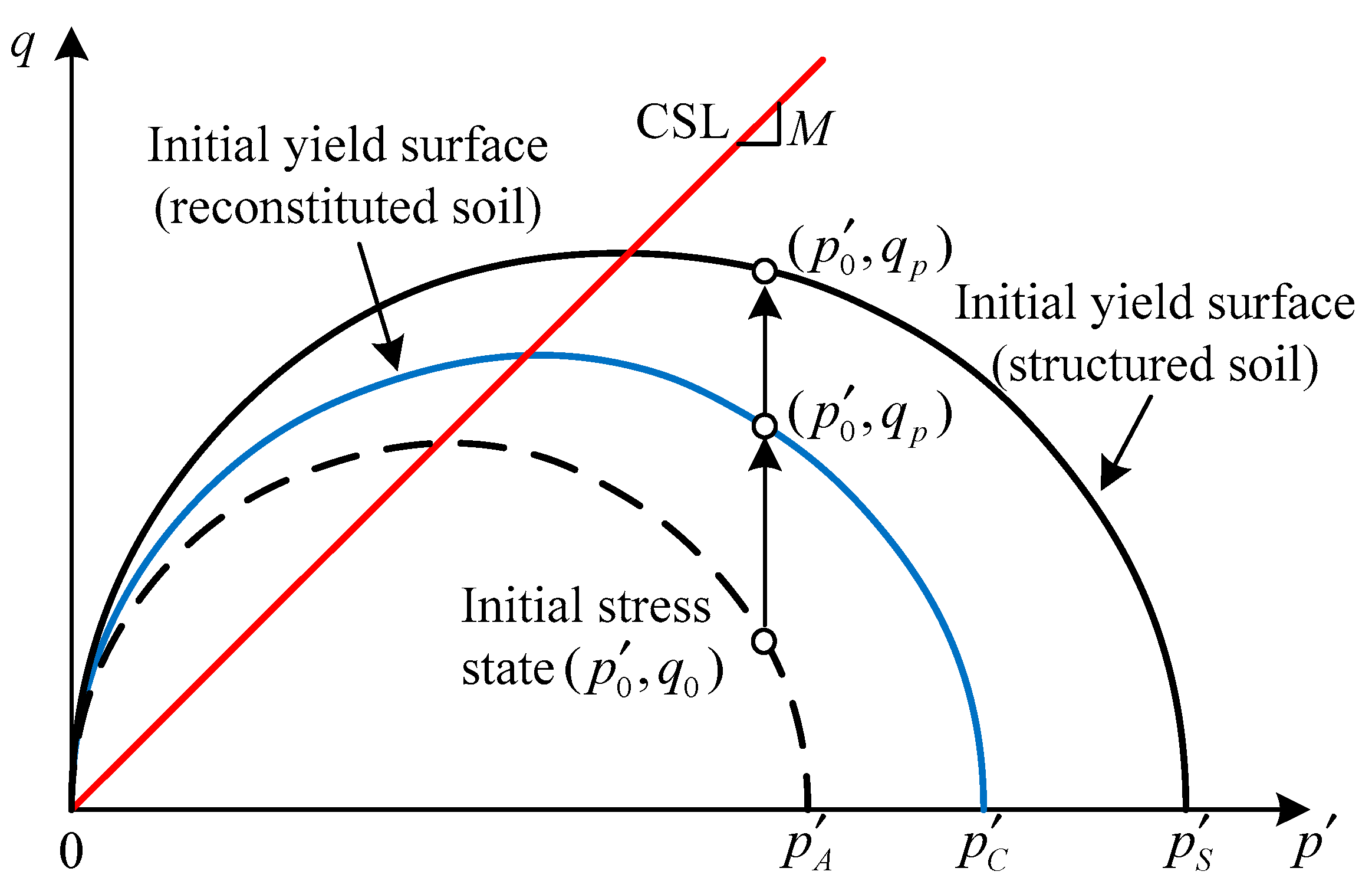
3.4. Initial Values at the Elastoplastic Boundary

To determine the initial values σ′_r(ξ_p), σ′_θ(ξ_p), and σ′_z(ξ_p), prior knowledge of the initial stress state and the degree of over-consolidation of structured soils is needed. As shown in Figure 4, (p₀, q₀) and (p₀, q_p) denote the initial stress point and initial yield stress point, respectively. The reference point is the size of a virtual yield surface passing through the point (p₀, q₀). The isotropic over-consolidation ratio of the reconstituted soils, R, is defined as by Chen and Abousleiman [22], which is different from the conventional over-consolidation ratio, OCR = σ′_v,max/σ′_v [6]. For structured soils, a higher stress level is required to reach the initial yield surface than that for the corresponding reconstituted soils due to $p_s^{\prime }>p_C^{\prime }$, which means that the structured soils exhibit partial ‘false’ over-consolidated behavior [34]. To denote the degree of structure, the initial structural ratio, R_s, is defined as follows:

$$R_s=\frac{p_s^{\prime }}{p_C^{\prime }}$$

(39)

It can be seen that R_s is greater than 1 for structured soils. When the soil is in a reconstituted state, $p_s^{\prime }$ equals $p_C^{\prime }$; therefore, R_s = 1. The stronger the initial structure, the greater R_s for the soils.

It should be mentioned that the stress components at the elastoplastic boundary r_p (corresponding to ξ = ξ_p) satisfy both the elastic solutions given by Equations (13)–(15) and the yield function given by Equation (2). Combining this with the definition of R_s, σ′_r(ξ_p), σ′_θ(ξ_p), and σ′_z(ξ_p) can be easily obtained following the method of Chen and Abousleiman [22]:

$${\sigma }_r^{\prime }({\xi }_p)={\sigma }_h^{\prime }+\sqrt{{{\sigma }_h^{\prime }}^2-(4{{\sigma }_h^{\prime }}^2+{{\sigma }_z^{\prime }}^2-2{\sigma }_h^{\prime }{\sigma }_z^{\prime }-q_p^2)/3}$$

(40)

$${\sigma }_r^{\prime }({\xi }_p)={\sigma }_h^{\prime }-\sqrt{{{\sigma }_h^{\prime }}^2-(4{{\sigma }_h^{\prime }}^2+{{\sigma }_z^{\prime }}^2-2{\sigma }_h^{\prime }{\sigma }_z^{\prime }-q_p^2)/3}$$

(41)

$${\sigma }_z^{\prime }({\xi }_p)={\sigma }_v^{\prime }$$

(42)

with

$${\xi }_p=\frac{{\sigma }_r^{\prime }({\xi }_p)-{\sigma }_h^{\prime }}{2G_0}$$

(43)

$$q_p=M{p}_0^{\prime }\sqrt{R{R}_s\left[1+\frac{1}{M^2}{\left(\frac{q_0}{p_0^{\prime }}\right)}^2\right]-1}$$

(44)

The initial values determined from Equations (40)–(44) are sufficient to solve the system of Equation (38a–c). Note that these equations are related to the auxiliary variable ξ; therefore, the obtained stress components vary with the ξ instead of the radial position r.

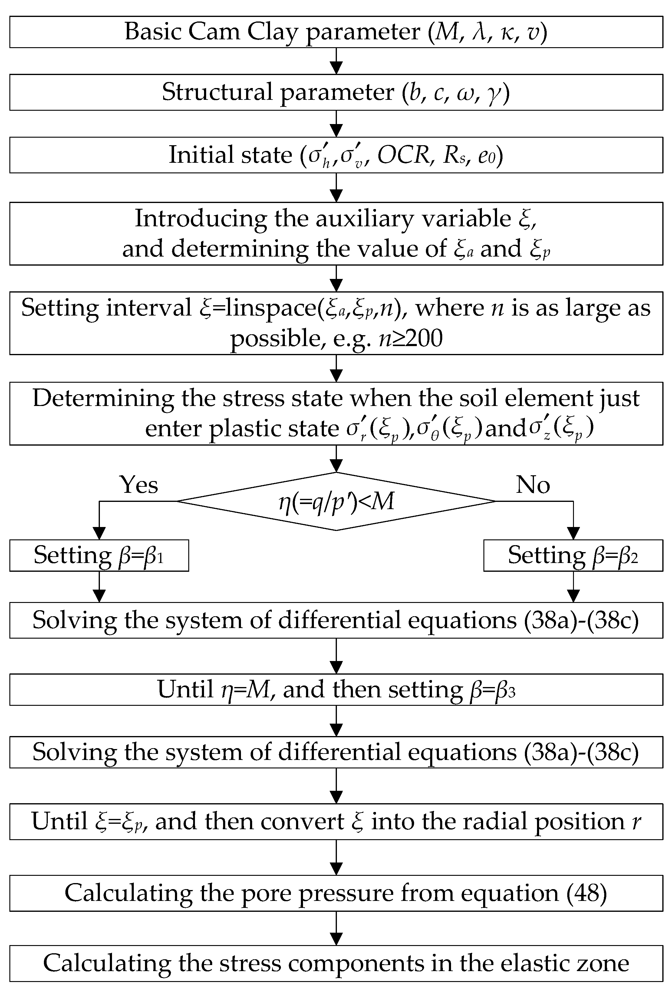
3.5. Determination of the Radial Position and Excess Pore Pressure

For the completeness of the present solution, the relationship between ξ and r needs to be established. For the undrained and plane-strain conditions, the incompressibility of the soil skeleton and pore fluid renders the current position of any soil element r as related to its initial position r₀, its initial cavity radius a₀, and its current cavity radius a, which can be formulated as

$$a^2-a_0^2=r^2-r_0^2$$

(45)

Combining Equation (45) with ξ = (r − r₀)/r, the relationship between ξ and r can be obtained as:

$$\frac{r}{a}=\sqrt{\frac{{\left(a_0/a\right)}^2-1}{{\left(1-\xi \right)}^2-1}}$$

(46)

In particular, the position of the elastoplastic boundary r_p can be obtained by setting ξ in Equation (46) as ξ_p, and then the explicit relationship between r_p and the cavity radii (a and a₀) can be written as

$$\frac{r_p}{a}=\sqrt{\frac{{\left(a_0/a\right)}^2-1}{{\left(\frac{{\sigma }_r^{\prime }({\xi }_p)-{\sigma }_h^{\prime }}{2G_0}\right)}^2-\frac{{\sigma }_r^{\prime }({\xi }_p)-{\sigma }_h^{\prime }}{G_0}}}$$

(47)

Once the effective stress variations are determined, the pore pressure u at any radial position r_x can be calculated from the equilibrium equation. By integrating Equation (10) from r_p to r_x, u is expressed as

$$u(r_x)=u_0+{\sigma }_{rp}^{\prime }-{\sigma }_{r_x}^{\prime }-{\displaystyle {\int }_{r_p}^{r_x}\frac{{\sigma }_r^{\prime }-{\sigma }_{\theta }^{\prime }}{r}}dr$$

(48)

Therefore, the excess pore pressure Δu(r_x) generated around the cavity can be easily obtained as u(r_x) − u₀.

4. Results and Discussion

Following the solution procedure shown in Figure 5, the present solution was implemented in the numerical software MATLAB 2018b. Firstly, the present solution was compared with the previous solutions both in reconstituted and structured soils [22,36]. Subsequently, parametric analyses were performed to investigate the cavity expansion responses for the soils with different structure degrees R_s and isotropic over-consolidation ratios R. Finally, the influences of the structural parameter on the cavity expansion responses were analyzed.

The present solution was performed in Boston Blue Clay because it has been widely used in the analyses of cavity expansion [22,23,24]. The basic Cam Clay parameters (M, λ, κ, v) and initial state parameters (R, σ_h, σ_v, e₀, G₀, and u₀) of Boston Blue Clay are listed in

Table 1. Soil property parameters used in calculation.

Basic Cam Clay Parameters				Structural Parameters
M	λ	κ	v	b	c	ω	γ
1.2	0.15	0.03	0.278	1	0	1	0.5

and

Table 2. Soil state parameters used in calculation.

R	σh (kPa)	σv (kPa)	e0	G0 (kPa)	u0 (kPa)
1	100	160	1.09	4348	100
1.2	100	160	1.06	4302	100
3	120	120	0.97	4113	100
10	144	72	0.80	3756	100

, respectively. Because of the absence of experimental data in the literature, the values of the structural parameters (b, c, ω, γ) were estimated in a reasonable range. In addition, three different initial structural ratios, R_s = 1.0, 1.2, and 1.5, were adopted, where the special case of R_s = 1.0, was chosen to highlight the difference between structured and reconstituted soils.

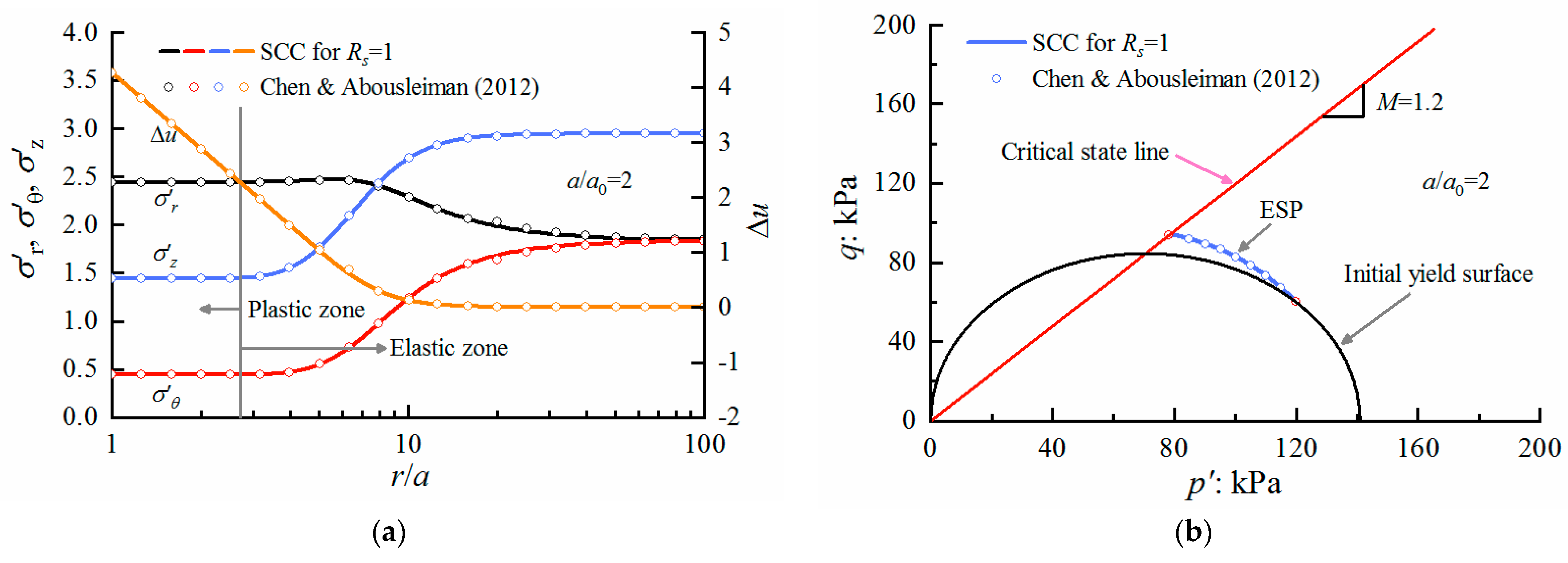
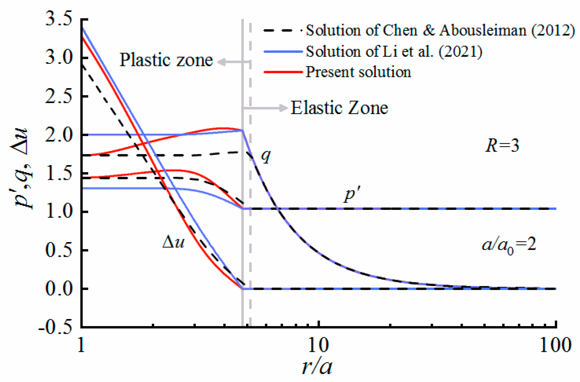
4.1. Comparisons between the Present Solution and Previous Solution

Theoretically, the existing undrained solution based on the MCC model [22] is a special case of the present solution based on the SCC model. This is because the SCC model can evolve to the MCC model by setting the relevant structural parameters as sufficiently small values, i.e., Δe→c, c→0, b→0, γ→0, and ω→0. In this situation, the initial yield surface of structured soils, as shown in Figure 4, tends to be the same as that of the corresponding reconstituted soils; therefore, the initial structural ratio R_s tends to be 1.

The present solution was implemented in the case of R_s→1, c→0, b→0, γ→0, and ω→0, and then compared with the existing undrained solution in reconstituted soils of Chen and Abousleiman [22], as shown in Figure 6. Note that only the initial state parameters of normally consolidated soils (R = 1) in Table 2 were adopted, and the stresses in Figure 6a were normalized by the undrained shear strength s_u (=54.3 kPa) for convenience of comparison. It can be seen that whether the distributions of the stress components along the radial distance, or the effective stress path for a soil element at the cavity wall, the results of present solution for structured soils are highly consistent with those of Chen and Abousleiman [22] for reconstituted soils. Thus, the solution proposed in this study can be regarded as a unified solution for undrained cavity expansion in structured and reconstituted soils.

The present solution was further compared with the undrained solution in structured soils proposed by Li et al. [36] to show the significances of destructuration. For the sake of convenience, the case of R = 3 in Table 2, which was calculated in [36], was selected, and all of the stresses were normalized by the undrained shear strength s_u (=115.0 kPa). Note that the same initial values at the elastoplastic boundary were adopted to ensure the soils containing the same initial structure. Figure 7 showed the comparisons of distributions of the mean effective stress p′, deviator stress q, and excess pore pressure Δu. It can be seen that soil structure has significant influences on the stress distributions around the cavity. Although the influences of the structure were considered in the solution of Li et al. [36], the values of p′ and q tends to be constant with the decrease of radial distance r/a in the plastic zone. This illustrated that only the initial structure was accounted for in their solution, and that the structure degradation was neglected, which resulted in the inability to capture the softening behavior caused by the destructuration. In contrast, the present solution could reflect the effects of structure degradation and crushing. Therefore, the p′ and q calculated in the present solution could finally reach the corresponding values in reconstituted soils at the cavity wall r/a = 1 after experiencing strain softening, indicating that the structure of the soils at the cavity wall was destroyed completely.

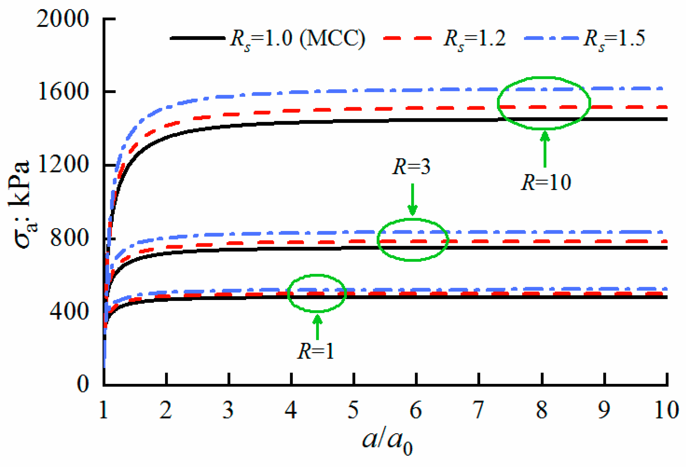
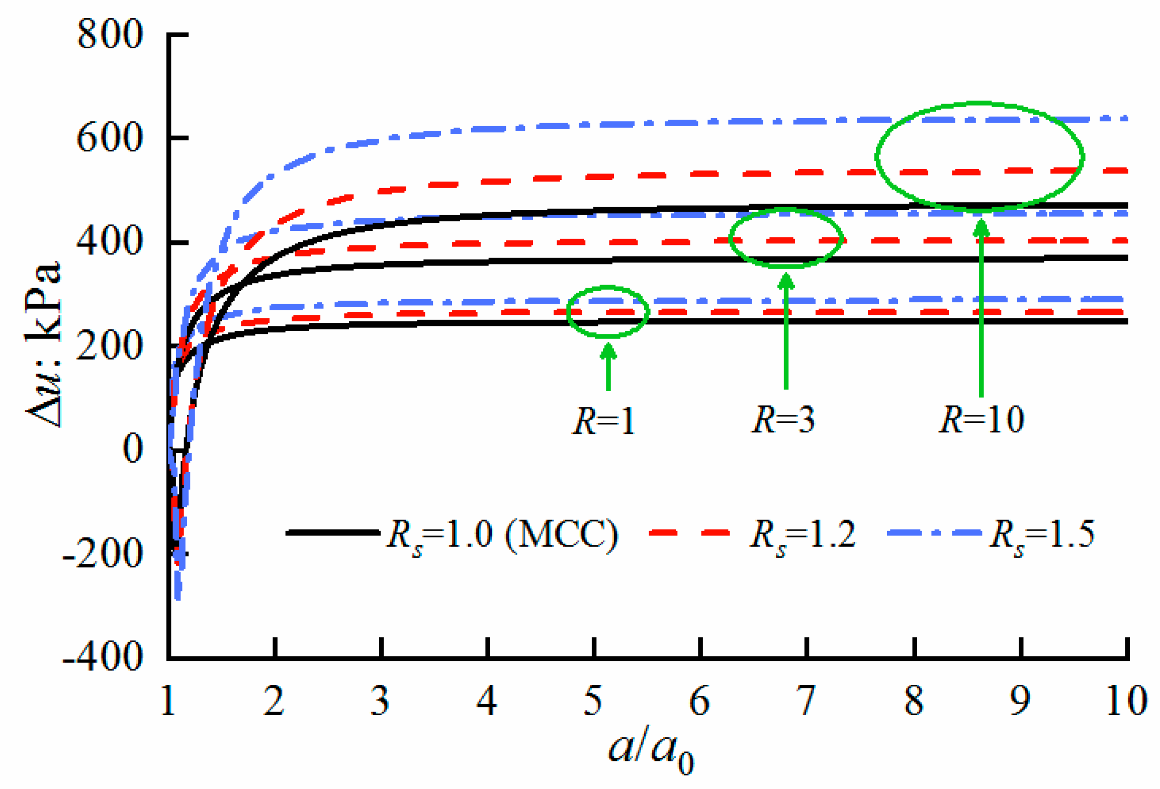
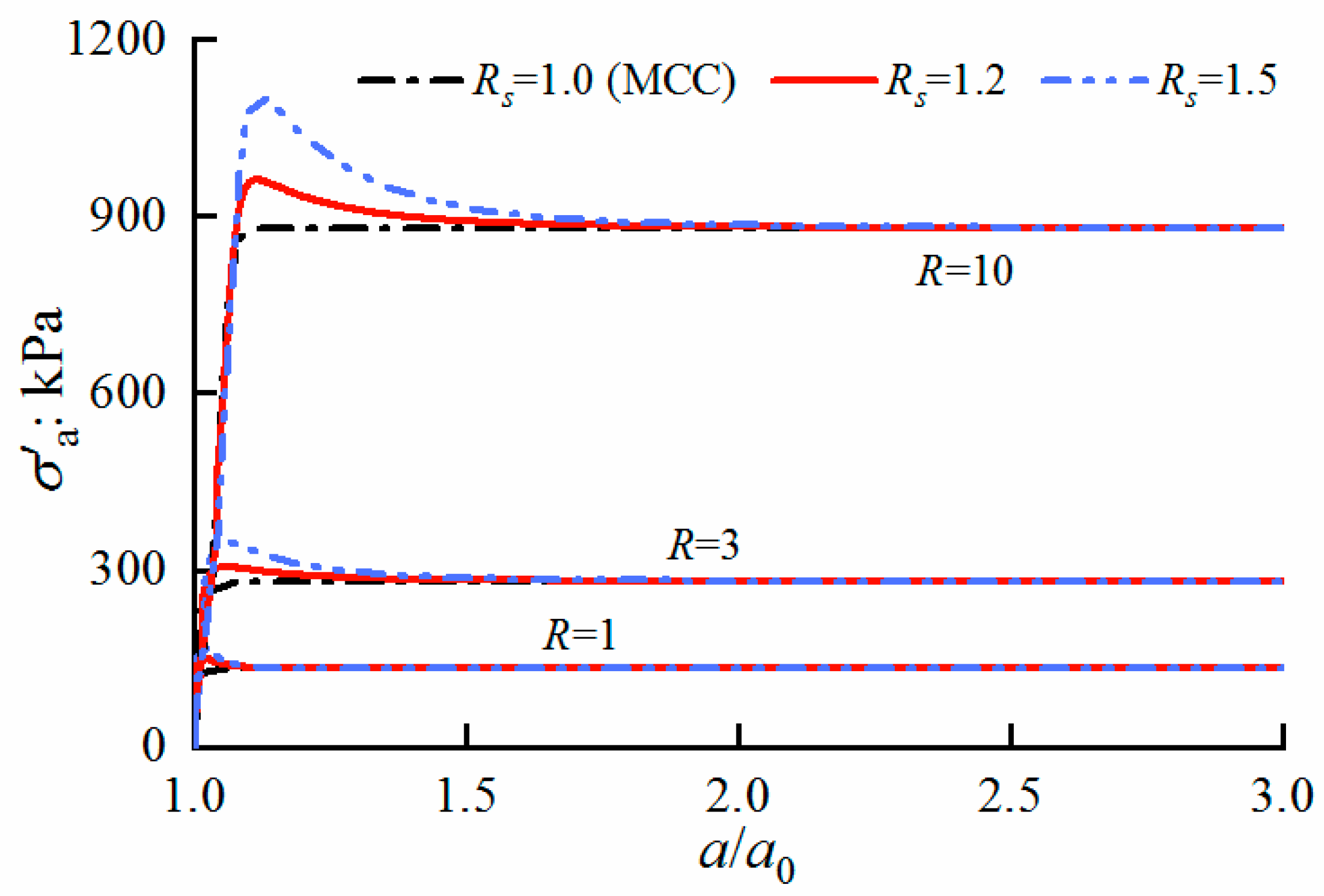
4.2. Internal Cavity Pressure and Excess Pore Pressure at the Cavity Wall

In this section, the characteristics of the cavity expansion curve (i.e., variations of the total and effective internal cavity pressure, σ_a and σ′_a) and the variations of excess pore pressure at the cavity wall were analyzed. Note that the results of R_s = 1.0 are equivalent to that of Chen and Abousleiman [22] (i.e., the results in the MCC model), which would be taken as a benchmark to highlight the influences of the initial structure and subsequent destructuration of soils on these variations.

As shown in Figure 8 and Figure 9, both the total internal cavity pressure σ_a and the excess pore pressure Δu increase sharply at the initial stage of cavity expansion, but then become slowly with an increase in a/a₀. When a/a₀ is greater than 5.0, both σ_a and Δu reach constant values. The comparisons between these results for soils with different R_s indicate that the structure has significant influences on the variations of σ_a and Δu. Specifically, the greater the R_s, the larger σ_a is required and the larger Δu will be generated when the cavity expands to the same a/a₀. In addition, for heavily over-consolidated soils (R = 10), a negative excess pore pressure is generated at the instant of cavity expansion, but it dissipates immediately with the further expansion, as shown in Figure 9.

The variations in the effective internal cavity pressure σ′_a with a/a₀ are plotted in Figure 10. For R_s = 1.0, the variation trends of σ′_a along a/a₀ are consistent with those of the total internal cavity pressure σ_a. For R_s = 1.2 and 1.5, σ′_a first increases to the peak values, and then decreases gradually with a further increase in a/a₀. Finally, σ′_a reaches the same value as that of the corresponding reconstituted soils (R_s = 1.0), although the peak value of σ′_a increases with R_s. The softening behavior of structured soils can be attributed to the release of accumulated stress due to the degradation and crushing of the structure. The same effective stress state is reached for the structured and the corresponding reconstituted soils, which indicates that the structure of soils at the cavity wall was completely destroyed. In fact, σ′_a can be calculated from the measured values of σ_a and Δu, which can be used to estimate the degree of destructuration for structured soils, as mentioned by Sivasithamparam and Castro [31].

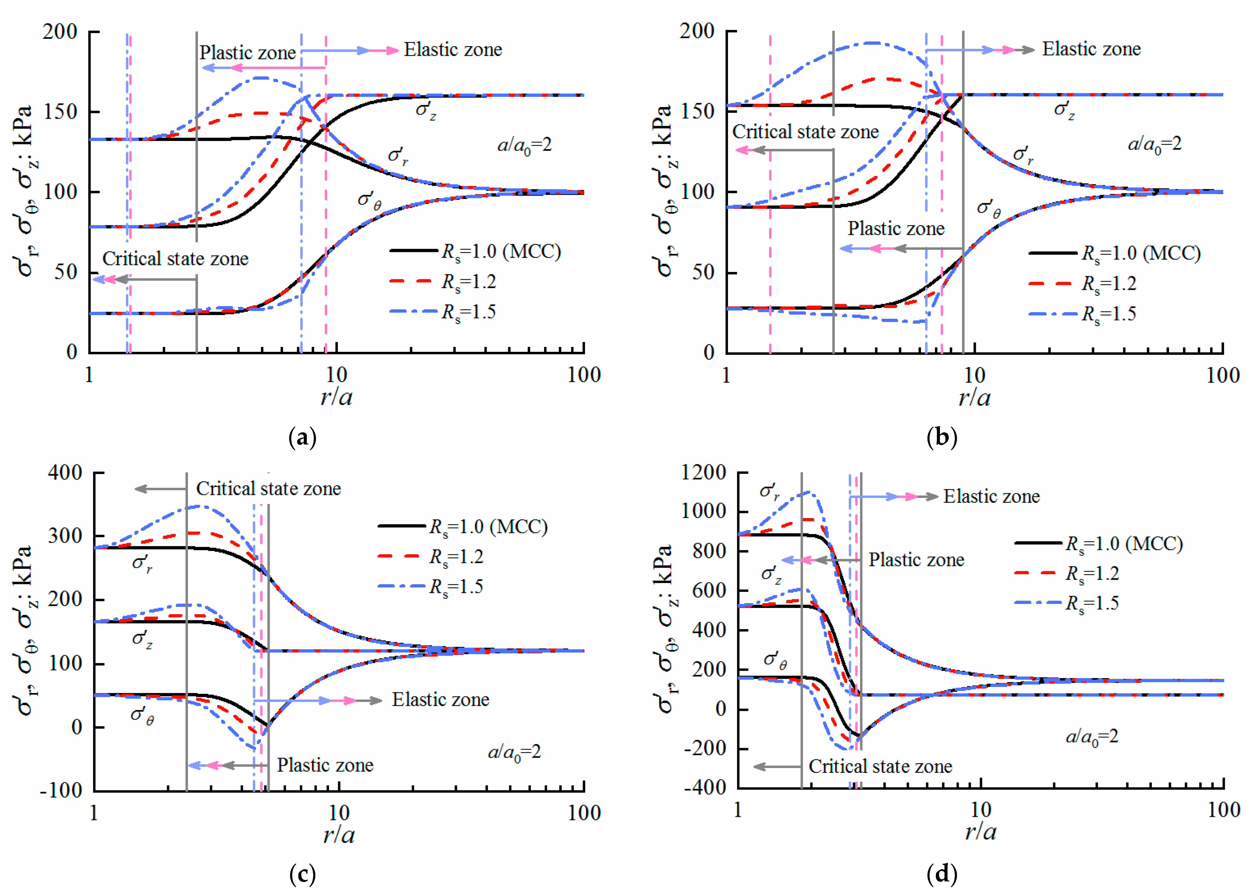
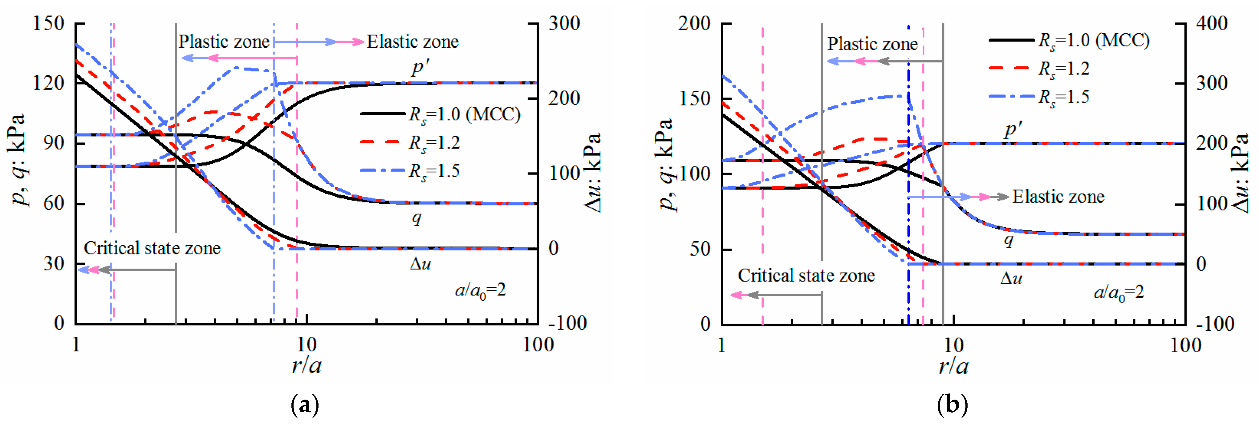
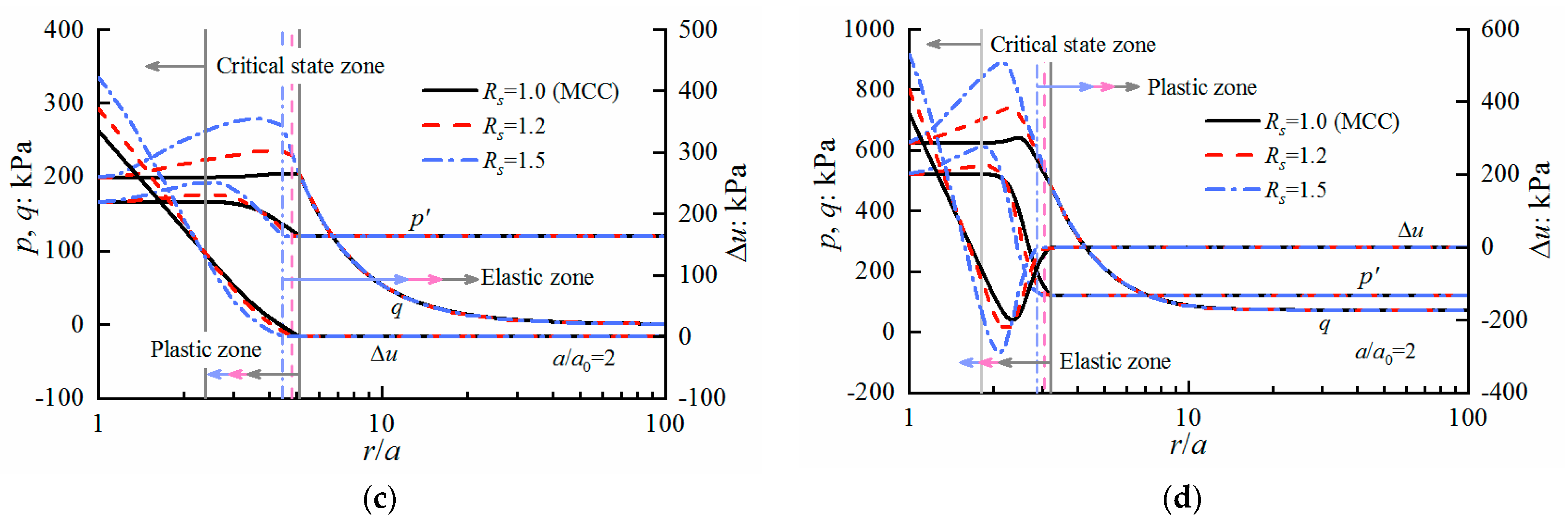
4.3. Distributions of Stress and Excess Pore Pressure around the Cavity

The stress distributions along the radial distance, including the stress components σ′_r, σ′_θ, σ′_z, mean effective stress p′, and deviator stress q, as well as the excess pore pressure Δu, are plotted in Figure 11 and Figure 12. These stress distributions at the instant of a/a₀ = 2 for R_s = 1.2 and 1.5 were also compared with those for R_s = 1.0 (i.e., the solution in [22]) to investigate the influences of the initial structure and the subsequent stress-induced destructuation. Note that, in these figures, the radial distance r is normalized by the current cavity radius a, and then plotted in logarithmic coordinates to highlight the stress features near the cavity.

From Figure 11, it can be seen that the distributions of σ′_r, σ′_θ, and σ′_z for R_s = 1.0, 1.2, and 1.5 are consistent in the far field but have significant differences in the near field around the cavity. According to the stress state, three zones, i.e., the elastic zone, plastic zone, and critical state zone, can be generally defined around the cavity. For reconstituted soils (R_s = 1.0), σ′_r, σ′_θ, and σ′_z vary monotonously in the plastic zone with a decrease in r/a, and tend to be constant in the critical state zone. For structured soils (R_s = 1.2, 1.5), σ′_r first increases to a maximum value corresponding to the peak strength of structured soils, and then decreases gradually with a decrease in r/a until the value is the same as that for R_s = 1.0. It can also be seen that the larger the R_s that is adopted, the larger the magnitudes of σ′_θ and σ′_z that are obtained in the plastic zone. However, the final critical state values are the same for structured and reconstituted soils, irrespective of the initial structure.

The influences of soil structure on the development of the stress-state zones around the expanding cavity can also be seen in Figure 11. For normal consolidated reconstituted soils (R = 1 with R_s = 1.0), there is no elastic zone, as shown in Figure 11a. However, for structured soils (R_s = 1.2, 1.5), the elastic zone appears because of the partial ‘false’ over-consolidated behavior of structured soils. For all cases, it can be seen that, as R_s increases, the position of the elastoplastic boundary gradually shifts to the left, the ranges of the plastic zone and critical state zone become narrow, and the critical state zone even disappears in some cases.

Figure 12 shows the distributions of the mean effective stress p′, the deviator stress q, as well as the excess pore pressure Δu around the cavity. It can be seen that, for reconstituted soils (R_s = 1.0), p′ and q remain almost unchanged in the vicinity of the cavity wall, which indicates that the soils have reached the critical state. As r/a increases, p′ and q may increase or decrease in the plastic zone, which actually depends on the values of R. For structured soils (R_s = 1.2 and 1.5), q increases rapidly with a decrease in r/a, and then decreases to a stable value with the destructuration of soils after reaching the peak value. The variations in p′ can be divided into two patterns, for normally consolidated and lightly over-consolidated soils (Figure 12a,b); p′ remains a constant in the elastic zone and decreases monotonously with the decrease in r/a during the plastic deformation. For moderately and heavily over-consolidated soils (Figure 12c,d), p′ increases to a peak value with the accumulation of the plastic strain and then decreases to the critical state value, which indicates that the soil undergoes plastic softening deformation after yielding.

Generally, when examining the stresses from the far field to the cavity wall, it is observed that the stresses for the soils with different R_s are consistent in the elastic zone, and that they then separate from each other approximately in the plastic zone, and finally come together again near the cavity wall. This is because the initial stresses for soils with a certain R and different R_s are the same, while the structure affects the stress responses of the soils and enhances the differences between structured and reconstituted soils. After the peak strength, the differences between the stress states of the soils with different R_s decrease and, finally, tend to be zero with the degradation and crushing of the structure.

It can also be seen that the variation trends of excess pore pressures Δu with r/a are similar for R_s = 1.0, 1.2, and 1.5, i.e., Δu remains zero in the elastic zone, and increases sharply and nearly linearly with the decrease in the logarithm of r/a in the plastic and critical zones. Meanwhile, the gradient of Δu versus lnr/a becomes larger for soils with larger R_s. For heavily over-consolidated soils (R = 10), negative excess pore pressures Δu are generated around the cavity, which illustrates that shear dilation occurs during cavity expansion.

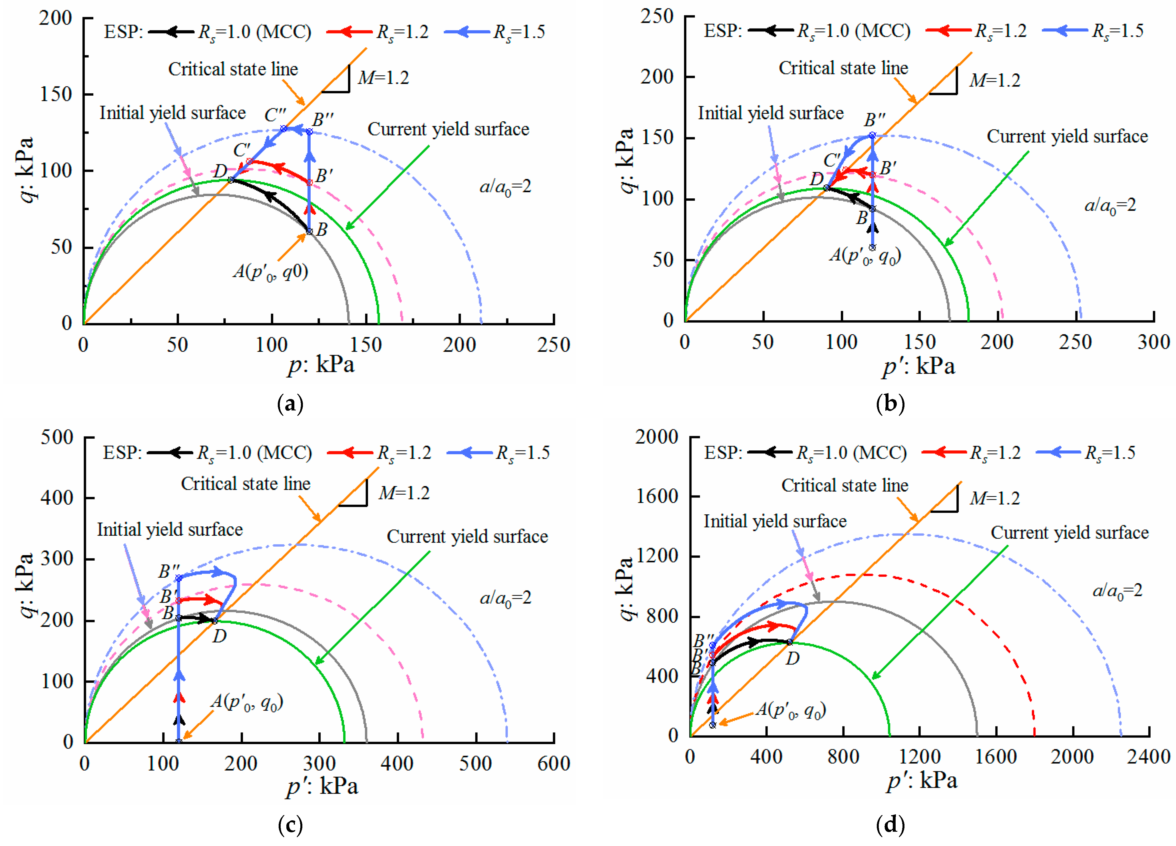
4.4. Stress Path for a Soil Element around the Cavity

For the soil element located at any position around the cavity, the same effective stress path (ESP) in p′–q plane is followed; therefore, only the ESP for a soil element at the cavity wall is analyzed. The ESPs for R = 1, 1.2, 3, and 10 are plotted in Figure 13, respectively. In these figures, points A, B, C, and D denote four stress variation points, i.e., the initial stress point (p₀, q₀), the initial yield stress point, the crushing beginning point, and the final critical state point, respectively. The B, B′, and B′′ were used to distinguish the initial yield stresses for R_s = 1.0, 1.2, and 1.5, respectively. Note that the comparisons of ESPs between the present solution and Chen and Abousleiman’s solution [22] were shown by comparing the case of R_s = 1.0 with that of R_s = 1.2 and 1.5.

From Figure 13, it is clear that the initial yield surface and yield stress increase as R_s increases. During the elastic deformation, the ESPs follow the vertical line until the stress state reaches the initial yield stress point B, B′, or B′′, except for the ESP for R = 1 with R_s = 1.0. Thereafter, the ESPs turn left or right with the development of plastic deformation, which depends on whether the soils experience hardening (the stress ratio at B, B′, or B′′ is smaller than M) or softening (the stress ratio at B, B′, or B′′ is larger than M).

For R_s = 1.0, the ESPs go monotonously to the left or right after the initial yielding, until the final critical state point D is reached. For R_s = 1.2 and 1.5, the ESPs turn left and reach the point C′ or C′′ when hardening occurs, and then travel along the CSL, owing to the structure crushing, until reaching the final critical state point D, as shown in Figure 11a,b. In contrast, the ESPs turn right and move toward the critical line when softening occurs, and then change their directions and travel downwards until they reach point D, as shown in Figure 13c,d. That the same point D is reached for the soils with different R_s indicates that the final critical state is irrespective of the initial structure, although it has significant influences on the ESPs, which can also be found in the shearing test results of structured soils [37]. In addition, it can be seen from Figure 13b that because of the ‘false’ over-consolidated behavior of structured soils, the slightly over-consolidated soils with R = 1.2 exhibit partial characteristics of the heavily over-consolidated soils when the R_s increases to 1.5, namely, the initial yield stress point B′′ was located at the left side of CSL, as shown in Figure 13b.

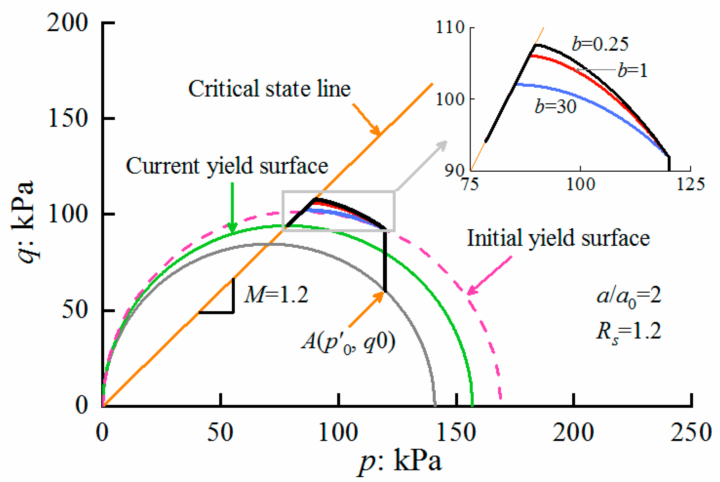
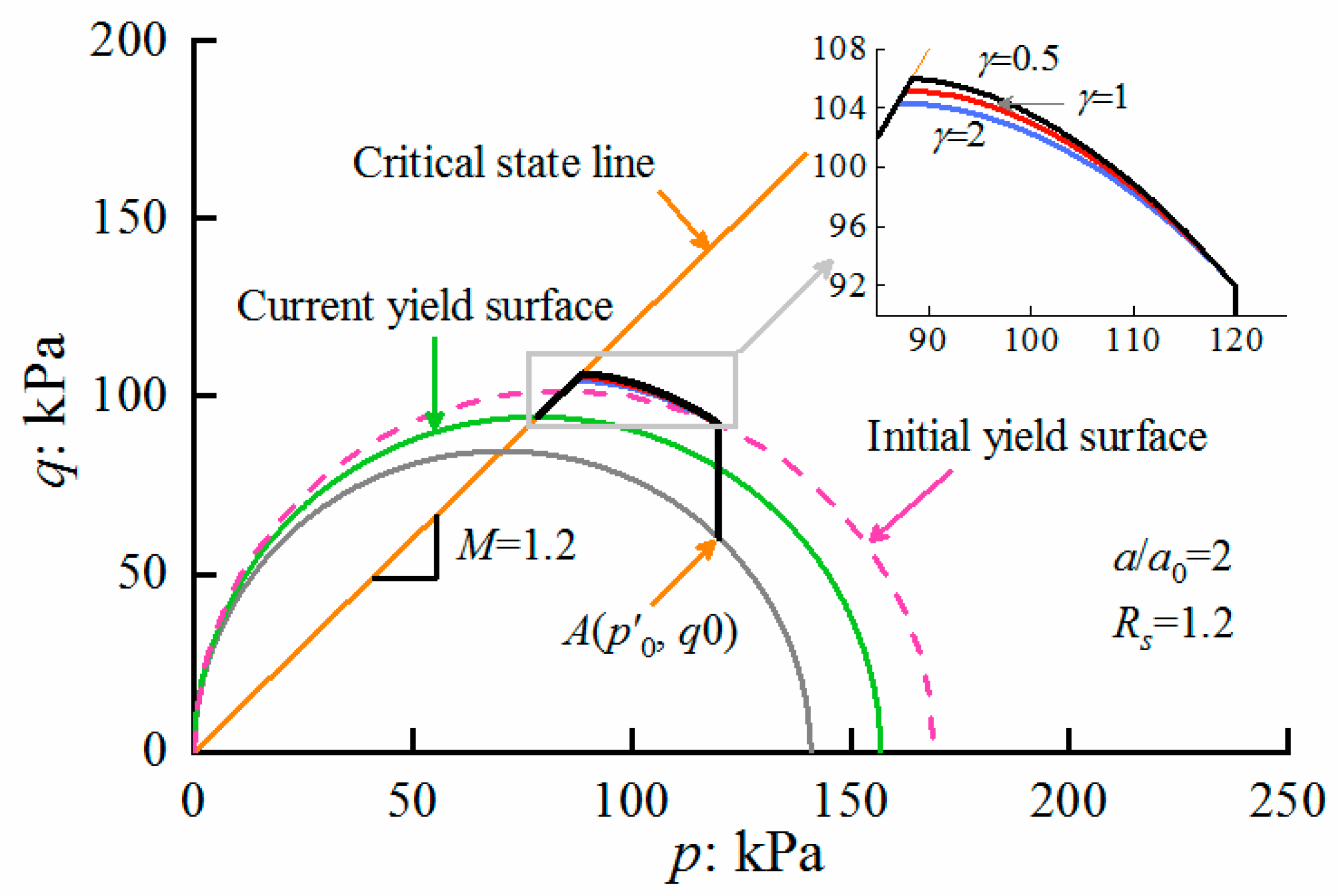
4.5. Influences of Structural Parameters

In this section, the influences of structural parameters (b, γ, c, ω) on the cavity expansion responses were further investigated. Herein, the soil property parameters in Table 1 and the state parameters in the case of R = 1 were chosen, and the calculation results were displayed in terms of effective stress path (ESP) in the p′–q plane.

The isotropic compression destructuring index b controls the decrease of the additional voids ratio Δe of structured soils, which represents the destructuration caused by the isotropic compression. As suggested by Carter and Liu [35], the values of b depend on soil structure and are generally b ≥ 1 for soft clay and b < 1 for stiff clays. Herein, b = 0.25, 1, and 30 were adopted to analyze the influences of b on the ESPs. The calculated results for b = 0.25, 1, and 30 were shown in Figure 14. As b increases, the ESP experiences a lower stress level, indicating that the stress release becomes more significant.

The shearing destructuring index γ reflects the influences of shear stress on the destructuration of soils. For the several natural and artificial structured soils reported in Carter and Liu [37], the values of γ are in the range of 0.5–2.1. Herein, γ = 0.5, 1, and 2 are adopted to analyze its influences on the cavity expansion responses. The calculation results are displayed in Figure 15, from which the same variation trends as Figure 14 can be observed. Obviously, γ together with b make prominent contributions to the destructuration of soils.

The structural parameter c is defined as the stable value of the additional voids ratio Δe when p′ is sufficiently large during the isotropic compression. Actually, the soil structure is almost completely removed under extremely large pressure, which means that the value of c is very small. Taking the natural Eastern Osaka Clay reported in Adachi et al. [42] as an example, Carter and Liu [37] concluded that the value of c for this clay can be assumed as zero. The parametric study shows that little differences occurred between various c values.

The structural parameter ω describes the flow rule, which is normally taken as 1 when the experimental data is insufficient, as suggested by Carter and Liu [37]. Actually, the values of ω also have little effect on the results.

5. Applications of Proposed Solution in Geotechnical Problems

In this section, two practical geotechnical problems are analyzed using the present solution. The first one is the jacking of a casing during the sand compaction pile installation, which is a typical penetration problem and is commonly modelled as the expansion of a cylindrical cavity. The second one is the in situ SBPM tests, in which the cylindrical probe is self-bored into soils to minimize the disturbance, and then the rubber membrane covering the probe expands the drilling.

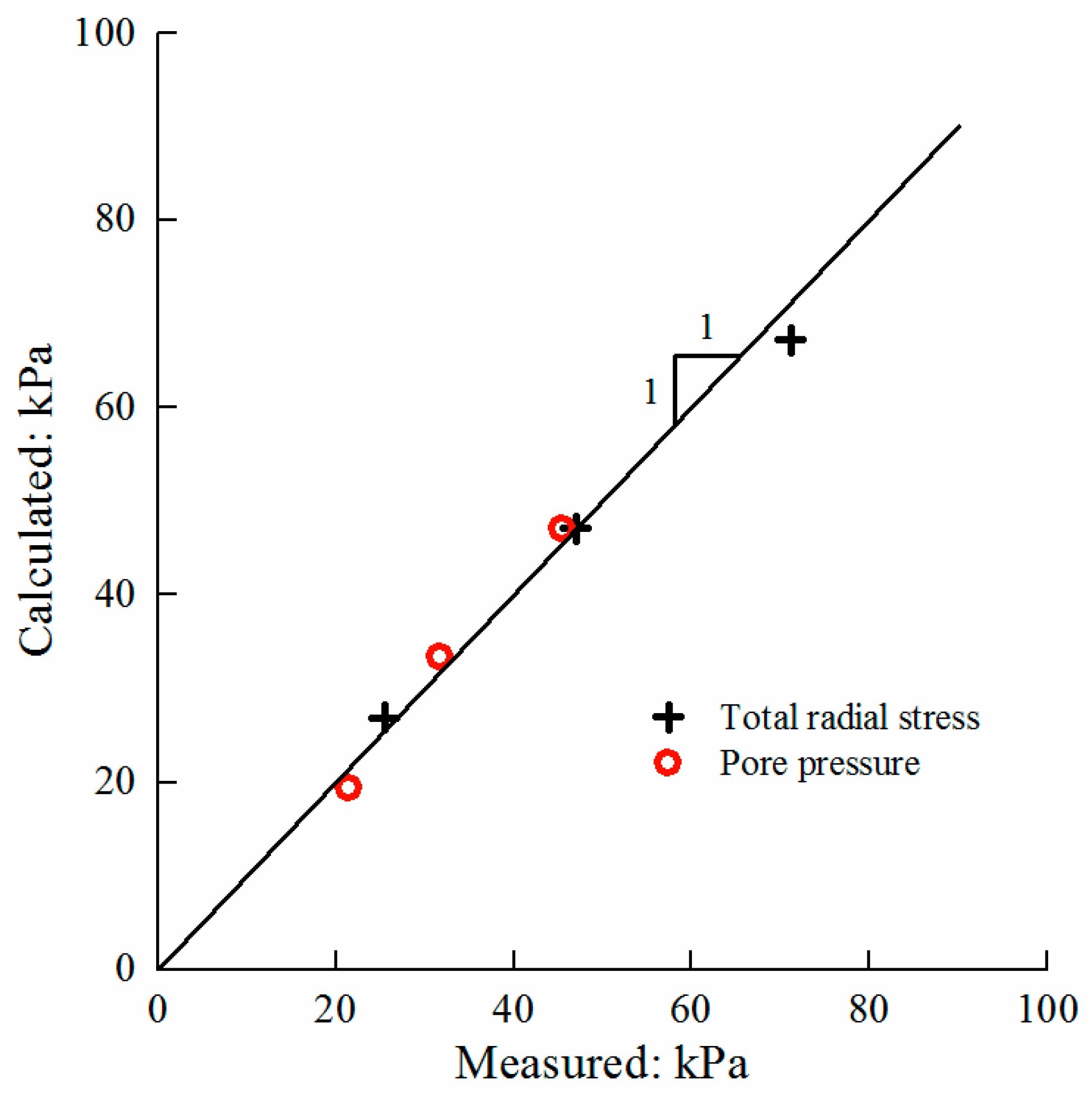
5.1. Estimation of Stress Variations Caused by the Casing Installation

Yi et al. [43] conducted a centrifuge model test to investigate the installation of a sand compaction pile. Before the ‘compacted’ sand column is formed, a cylindrical casing is jacked into the reconstituted Malaysian Kaolin clay, in which the water level is 0.25-m (prototype scale) higher than the ground. In centrifuge modelling, the total stress and pore pressure transducers were inserted at 4.6 times the casing radius and at prototype depths of 1.5 m, 2.75 m, and 4 m. The measured total radial stress and pore pressure at the instant of the casing tip’s arrival at these specific depths was extracted.

The present solution was used to predict the variations of total radial stress and pore pressure caused by the casing installation. The parameters of Malaysian Kaolin clay are taken from Purwana et al. [44] and Yi et al. [43]. The basic Modified Cam Clay parameters are M = 0.9, λ = 0.244, κ = 0.053, e^*_IC = 2.35, and v = 0.33. The lateral stress coefficient K₀ and effective unit weight γ′ are 0.6 and 6 kN/m³, respectively. The initial shear modulus G₀ is taken as 20p′₀, as in Yi et al. [43]. The Malaysian Kaolin clay used in the centrifuge model test is reconstituted; therefore, it is reasonable to take the structural parameters (b, γ, c, ω) as sufficiently small. Because there was no cavity existing before the casing was jacked, the value of a/a₀ should be set large enough (larger than 5, see Figure 8) so that the cavity pressure is stable.

Taking the above parameters as input data, the distribution of effective radial stress and pore pressure can be obtained. According to the location of the transducers (at the radial distance r/a = 4.6), the predicted radial effective stress and excess pore pressure was extracted from the stress distribution. The predicted stresses were compared with the corresponding measured values, as shown in Figure 16. It can be seen that the stress variations caused by the casing installation can be well predicted by the present solution.

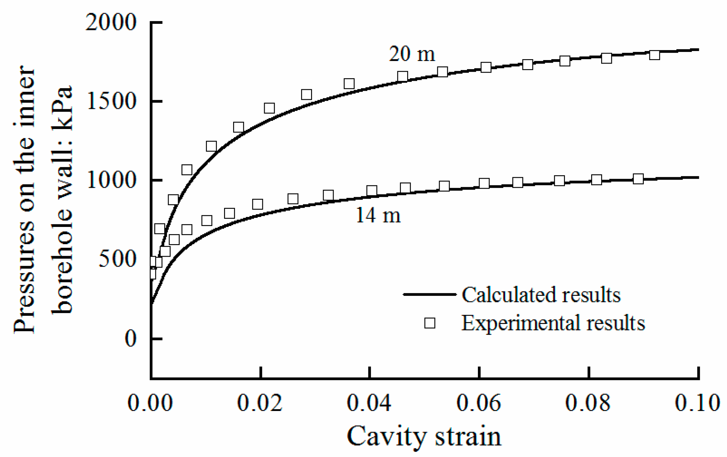
5.2. Interpretation of Pressuremeter Tests

The in situ SBPM test results reported by Rouainia et al. [45] were selected to further illustrate the applicability of the present solution in structured soils. These SBPM tests were performed at depths of 14 m and 20 m in London Clay, and the relationships between the cavity strain and pressure on the inner borehole wall were well documented.

The relevant parameters of London Clay can be found from Gasparre and Coop [46] and Rouainia et al. [45], i.e., M = 0.87, λ = 0.097, κ = 0.003, v = 0.3. The bulk unit weight below the water table (5.6-m depth at the test site) is 20 kN/m³. The over-consolidation ratio at the depths 14 m and 20 m are 3.0 and 4.0, respectively. According to the isotropic compression test results, the values of $e_{IC}^{\ast }$ is estimated to be 1.4. The lateral stress coefficients for normally consolidated and over-consolidated conditions are estimated using [47]:

$$K_{0nc}=1-\sin {\phi }^{\prime }$$

(49)

$$K_{0oc}=K_{0nc}OC{R}^{\sin {\phi }^{\prime }}$$

(50)

where φ′ is the effective friction angle. For London Clay, φ′ varies in the range of 20–25° [48], and its average value is adopted here.

As suggested by Liu and Carter [35], the value of b is smaller than 1 for stiff clays, and therefore, 0.8 is adopted for the stiff London Clay in the calculation. The values of c, γ, and ω refer to Carter and Liu [37], and are taken as 0.005, 1.0, and 1.5. Because the initial structure is enhanced with depth, R_s = 3.0 and 3.2 are adopted for 14 m and 20 m, respectively.

The variations of the pressure on the inner borehole wall with the cavity strain were predicted using the present solution. Adopting the aforementioned parameters, the relationships between the total internal cavity pressure and cavity radial can be calculated using the present solution, as shown in Figure 8. It is known that the pressure applied by the probe to the inner borehole wall is equivalent to the total internal cavity pressure, and the cavity strain is (a − a₀)/a₀. Thus, the results of SBPM tests can be predicated from the cavity expansion curves by converting the cavity radius into the cavity strain. As shown in Figure 17, the general trend of SBPM test response curves are well captured, and the present solution predicted a pressure on the inner borehole wall very close to the measured data from the SBPM tests.

6. Conclusions

For the problem of cylindrical cavity expansion in naturally structured soils, an undrained elastoplastic solution was presented by using the SCC model of Carter and Liu [37]. Although the flow rules in the SCC model follow the different forms during the hardening, softening, and crushing processes, a unified system of differential equations was established for the considered problem, which can be solved in a simplified procedure by introducing an auxiliary variable. The present solution was compared with the previous solutions in reconstituted and structured soils to show the validity and significances of this study. Subsequently, parametric studies were conducted to explore the characteristics of cavity expansion responses in the structured soils, and then the influences of structural parameters were investigated. Finally, the casing installation and in situ SBPM tests were analyzed using the present solution. The following conclusions were drawn:

(1)

Because the initial structure and destructuration effects are sufficiently considered, the present solution is capable of capturing the typical mechanical responses of naturally structured soils around the cavity. With the increase of the initial structure, the yielding stress increases and the ‘false’ over-consolidated behavior is strengthened. Moreover, as a result of the destructuration, the soils with different initial structures will reach the same critical state when the structure is completely destroyed;

(2)

The soil structure has significant influences on the cavity responses. As the cavity expands, the effective internal cavity pressure and the deviatoric stress decreases rapidly once the peak values are reached, which can be attributed to the release of accumulated stress due to the degradation and crushing of the structure;

(3)

The present solution can evolve to the existing solution in reconstituted soils when the structural parameters are sufficiently small. Therefore, the present solution can be regarded as a unified solution for cavity expansion in structured and reconstituted soils;

(4)

Compared with the previous solutions, the present solution takes the destructuration into account and captures the softening behavior of natural soils well;

(5)

The simulations of the casing installation and in situ self-boring pressuremeter tests indicate that the present solution provides an effective theoretical tool for the analyses of practical geotechnical problems involving cylindrical cavity expansion.

References

1. Yu, H.S. Cavity Expansion Methods in Geomechanics; Kluwer Academic Publishers: Dordrecht, The Netherlands, 2000. [Google Scholar] [CrossRef]
2. Vesic, A.S. Expansion of cavities in infinite soil mass. J. Soil Mech. Found. Div. Am. Soc. Civ. Eng. 1972, 98, 265–290. [Google Scholar] [CrossRef]
3. Chang, M.F.; Teh, C.I.; Cao, L.F. Undrained cavity expansion in modified Cam clay II: Application to the interpretation of the piezocone test. Geotechnique 2001, 51, 335–350. [Google Scholar] [CrossRef]
4. Cudmani, R.; Osinov, V.A. The cavity expansion problem for the interpretation of cone penetration and pressuremeter tests. Can. Geotech. J. 2001, 38, 622–638. [Google Scholar] [CrossRef]
5. Carter, J.P.; Randolph, M.F.; Wroth, C.P. Stress and pore pressure changes in clay during and after the expansion of a cylindrical cavity. Int. J. Numer. Anal. Methods Geomech. 1979, 3, 305–322. [Google Scholar] [CrossRef]
6. Randolph, M.F.; Carter, J.P.; Wroth, C.P. Driven piles in clay-the effects of installation and subsequent consolidation. Geotechnique 1979, 29, 361–393. [Google Scholar] [CrossRef] [Green Version]
7. Lee, F.H.; Juneja, A.; Tan, T.S. Stress and pore pressure changes due to sand compaction pile installation in soft clay. Geotechnique 2004, 54, 1–16. [Google Scholar] [CrossRef]
8. Yu, H.S.; Rowe, R.K. Plasticity solutions for soil behavior around contracting cavities and tunnels. Int. J. Numer. Anal. Methods Geomech. 1999, 23, 1245–1279. [Google Scholar] [CrossRef]
9. Chen, S.L.; Abousleiman, Y.N. Drained and undrained analyses of cylindrical cavity contractions by bounding surface plasticity. Can. Geotech. J. 2016, 53, 1398–1411. [Google Scholar] [CrossRef] [Green Version]
10. Mo, P.Q.; Yu, H.S. Undrained cavity contraction analysis for prediction of soil behavior around tunnels. Int. J. Geomech. 2017, 17, 04016121. [Google Scholar] [CrossRef] [Green Version]
11. Liu, K.; Chen, S.L.; Gu, X.Q. Analytical and numerical analyses of tunnel excavation problem using an extended drucker-prager model. Rock Mech. Rock Eng. 2020, 53, 1777–1790. [Google Scholar] [CrossRef]
12. Chen, S.L.; Liu, K. Undrained cylindrical cavity expansion in anisotropic critical state soils. Geotechnique 2018, 69, 189–202. [Google Scholar] [CrossRef]
13. Carter, J.P.; Booker, J.R.; Yeung, S.K. Cavity expansion in cohesive frictional soils. Geotechnique 1986, 36, 349–358. [Google Scholar] [CrossRef]
14. Yu, H.S.; Houlsby, G.T. Finite cavity expansion in dilatants soils: Loading analysis. Geotechnique 1991, 41, 173–183. [Google Scholar] [CrossRef]
15. Durban, D.; Fleck, N.A. Spherical cavity expansion in a Drucker-Prager solid. J. Appl. Mech. 1997, 64, 743–750. [Google Scholar] [CrossRef]
16. Cao, L.F.; Teh, C.I.; Chang, M.F. Undrained cavity expansion in modified Cam clay I: Theoretical analysis. Geotechnique 2001, 51, 323–334. [Google Scholar] [CrossRef]
17. Collins, I.F.; Stimpson, J.R. Similarity solutions for drained and undrained cavity expansions in soils. Geotechnique 1994, 44, 21–34. [Google Scholar] [CrossRef]
18. Russell, A.R.; Khalili, N. On the problem of cavity expansion in unsaturated soils. Comput. Mech. 2006, 37, 311–330. [Google Scholar] [CrossRef]
19. Yang, H.W.; Russell, A.R. Cavity expansion in unsaturated soils exhibiting hydraulic hysteresis considering three drainage conditions. Int. J. Numer. Anal. Methods Geomech. 2015, 39, 1975–2016. [Google Scholar] [CrossRef]
20. Mo, P.Q.; Yu, H.S. Undrained cavity expansion analysis with a unifed state parameter model for clay and sand. Geotechnique 2016, 67, 503–515. [Google Scholar] [CrossRef]
21. Zhou, H.; Kong, G.Q.; Liu, H.L.; Laloui, L. Similarity solution for cavity expansion in thermoplastic soil. Int. J. Numer. Anal. Meth. Geomech. 2018, 42, 274–294. [Google Scholar] [CrossRef]
22. Chen, S.L.; Abousleiman, Y.N. Exact undrained elasto-plastic solution for cylindrical cavity expansion in modified Cam Clay soil. Geotechnique 2012, 62, 447–456. [Google Scholar] [CrossRef]
23. Chen, S.L.; Abousleiman, Y.N. Exact drained solution for cylindrical cavity expansion in modified Cam Clay soil. Geotechnique 2013, 63, 510–517. [Google Scholar] [CrossRef]
24. Li, L.; Li, J.P.; Sun, D.A. Anisotropically elasto-plastic solution to undrained cylindrical cavity expansion in K0-consolidated clay. Comput. Geotech. 2016, 73, 83–90. [Google Scholar] [CrossRef]
25. Sivasithamparam, N.; Castro, J. Undrained expansion of a cylindrical cavity in clays with fabric anisotropy: Theoretical solution. Acta Geotech. 2018, 13, 729–746. [Google Scholar] [CrossRef]
26. Yang, C.Y.; Li, J.P.; Li, L.; Sun, D.A. Expansion responses of a cylindrical cavity in overconsolidated unsaturated soils: A semi-analytical elastoplastic solution. Comput. Geotech. 2020, 130, 103922. [Google Scholar] [CrossRef]
27. Chen, H.H.; Li, L.; Li, J.P.; Sun, D.A. Elastoplastic solutions for cylindrical cavity expansion in unsaturated soils. Comput. Geotech. 2020, 123, 103569. [Google Scholar] [CrossRef]
28. Taiebat, M.; Dafalias, Y.F.; Peek, R. A destructuration theory and its application to SANICLAY model. Int. J. Numer. Anal. Meth. Geomech. 2009, 34, 1009–1040. [Google Scholar] [CrossRef] [Green Version]
29. Mantaras, F.M.; Schnaid, F. Cylindrical cavity expansion in dilatant cohesivefrictional materials. Geotechnique 2002, 52, 337–348. [Google Scholar] [CrossRef]
30. Schnaid, F.; Mantaras, F.M. Cavity expansion in cemented materials: Structure degradation effects. Geotechnique 2003, 53, 797–807. [Google Scholar] [CrossRef]
31. Sivasithamparam, N.; Castro, J. Undrained cylindrical cavity expansion in clays with fabric anisotropy and structure: Theoretical solution. Comput. Geotech. 2020, 120, 103386. [Google Scholar] [CrossRef]
32. Wheeler, S.J.; Naatanen, A.; Karstunen, M.; Lojander, M. An anisotropic elastoplastic model for soft clays. Can. Geotech. J. 2003, 40, 403–418. [Google Scholar] [CrossRef]
33. Karstunen, M.; Krenn, H.; Wheeler, S.J.; Koskinen, M.; Zentar, R. Effect of anisotropy and destructuration on the behaviour of Murro test embankment. Int. J. Geomech. 2005, 9, 87–97. [Google Scholar] [CrossRef]
34. Li, J.P.; Zhou, P.; Li, L.; Xie, F. Elastoplastic solution of drained expansion of a cylindrical cavity in structured soils considering structure degradation. Comput. Geotech. 2021, 133, 104051. [Google Scholar] [CrossRef]
35. Liu, M.D.; Carter, J.P. A structured Cam Clay model. Can. Geotech. J. 2002, 39, 1313–1332. [Google Scholar] [CrossRef] [Green Version]
36. Li, J.P.; Zhou, P.; Li, L.; Xie, F.; Cui, J.F. Elastic-plastic solution for undrained expansion of cylindrical cavity in saturated structured loess. J. Tongji Univ. (Nat. Sci.) 2021, 49, 163–172. (In Chinese) [Google Scholar] [CrossRef]
37. Carter, J.P.; Liu, M.D. Review of the Structured Cam Clay Model. In Soil Constitutive Model: Evaluation, Selection and Calibration; ASCE, Geotechnical Special Publication: Reston, VA, USA, 2005; pp. 99–132. [Google Scholar] [CrossRef]
38. Horpibulsuk, S.; Liu, M.D.; Liyanapathirana, D.S.; Suebsuk, J. Behaviour of cemented clay simulated via the theoretical framework of the Structured Cam Clay model. Comput. Geotech. 2010, 37, 1–9. [Google Scholar] [CrossRef]
39. Burland, J.B. On the compressibility and shear strength of natural clays. Geotechnique 1990, 40, 329–378. [Google Scholar] [CrossRef]
40. Cotecchia, F.; Chandler, R.J. The influence of structure on the pre-failure behavior of a natural clay. Geotechnique 1997, 47, 523–544. [Google Scholar] [CrossRef]
41. Wood, D.M. Soil Behavior and Critical State Soil Mechanics; Cambridge University Press: Cambridge, UK, 1990. [Google Scholar]
42. Adachi, T.; Oka, F.; Hirata, T.; Hashimoto, T.; Nagaya, J.; Mimura, M.; Pradhan, T.B.S. Stress-strain behaviour and yielding characteristics of Eastern Osaka clay. Soils Found. 1995, 35, 1–13. [Google Scholar] [CrossRef] [Green Version]
43. Yi, J.T.; Goh, S.H.; Lee, F.H. Effect of sand compaction pile installation on strength of soft clay. Geotechnique 2013, 63, 1029–1041. [Google Scholar] [CrossRef]
44. Purwana, O.A.; Leung, C.F.; Chow, Y.K.; Foo, K.S. Influence of base suction on extraction of jack-up spudcans. Géotechnique 2005, 55, 741–753. [Google Scholar] [CrossRef]
45. Rouainia, M.; Panayides, S.; Arroyo, M.; Gens, A. A pressuremeter-based evaluation of structure in London Clay using a kinematic hardening constitutive model. Acta Geotech. 2020, 15, 2089–2101. [Google Scholar] [CrossRef] [Green Version]
46. Gasparre, A.; Coop, M.R. Quantification of the effects of structure on the compression of a stiff clay. Can. Geotech. J. 2008, 45, 1324–1334. [Google Scholar] [CrossRef]
47. Chang, M.F.; Teh, C.I.; Cao, L.F. Critical state strength parameters of saturated clays from the modified Cam clay model. Rev. Can. Géotechnique 1999, 36, 876–890. [Google Scholar] [CrossRef]
48. Avgerinos, V.; Potts, D.M.; Standing, J.R. The use of kinematic hardening models for predicting tunnelling-induced ground movements in London Clay. Geotechnique 2016, 66, 106–120. [Google Scholar] [CrossRef] [Green Version]
Figure 1. Conceptual model of soil responses under isotropic compression.
Applsci 12 00440 g001
Figure 2. Yield surfaces of the structured Cam Clay soil.
Applsci 12 00440 g002
Figure 3. Mechanical model for undrained cylindrical cavity expansion in the SCC soil.
Applsci 12 00440 g003
Figure 4. Elastic stress trajectory and over-consolidation ratio of structured soils.
Applsci 12 00440 g004
Figure 5. The flowchart for solving the cavity expansion problem using the present solution.
Applsci 12 00440 g005
Figure 6. Comparison between the present solution and existing solution in reconstituted soils: (a) distributions of σr, σθ, σz, and Δu along r/a; (b) the p′–q stress path.
Applsci 12 00440 g006
Figure 7. Comparison between the present solution and the previous solutions: distributions of p′, q, and Δu along r/a.
Applsci 12 00440 g007
Figure 8. Relationship between the total internal cavity pressure σa and the cavity radius a/a0.
Applsci 12 00440 g008
Figure 9. Relationship between the excess pore pressure Δu and the cavity radius a/a0.
Applsci 12 00440 g009
Figure 10. Relationship between the effective internal cavity pressure σa and the cavity radius a/a0.
Applsci 12 00440 g010
Figure 11. Influences of initial structure and destructuration on the distributions of effective stress components σr, σθ, and σz around the cavity: (a) R = 1; (b) R = 1.2; (c) R = 3; (d) R = 10.
Applsci 12 00440 g011
Figure 12. Influences of initial structure and destructuration on the distributions of p′, q and Δu around the cavity: (a) R = 1; (b) R = 1.2; (c) R = 3; (d) R = 10.
Applsci 12 00440 g012aApplsci 12 00440 g012b
Figure 13. Effective stress paths for the structured and the corresponding reconstituted soils: (a) R = 1; (b) R = 1.2; (c) R = 3; (d) R = 10.
Applsci 12 00440 g013
Figure 14. Effects of structural parameter b on the effective stress paths.
Applsci 12 00440 g014
Figure 15. Effects of structural parameter γ on the effective stress paths.
Applsci 12 00440 g015
Figure 16. Calculated against measured total radial stress and pore pressure during the casing installation.
Applsci 12 00440 g016
Figure 17. Comparisons of calculated and experimental results for the SBPM tests: cavity strain pressure on the inner borehole wall.
Applsci 12 00440 g017