
Toward Optimal Control of a Multivariable Magnetic Levitation System


Faculty of Electrical Engineering, Automatic Control and Informatics, Opole University of Technology, Prószkowska 76 Street, 45-758 Opole, Poland
*
Author to whom correspondence should be addressed.
Appl. Sci. 2022, 12(2), 674; https://0-doi-org.brum.beds.ac.uk/10.3390/app12020674
Submission received: 13 December 2021
/
Revised: 30 December 2021
/
Accepted: 4 January 2022
/
Published: 11 January 2022
(This article belongs to the Special Issue New Trends in Automation Control Systems and Their Applications)
Abstract
:In the paper, a comparative case study covering different control strategies of unstable and nonlinear magnetic levitation process is investigated. Three control procedures are examined in order to fulfill the specified performance indices. Thus, a dedicated PD regulator along with the hybrid fuzzy logic PID one as well as feed-forward neural network regulator are respected and summarized according to generally understood tuning techniques. It should be emphasized that the second PID controller is strictly derived from both arbitrary chosen membership functions and those ones selected through the genetic algorithm mechanism. Simulation examples have successfully confirmed the correctness of obtained results, especially in terms of entire control process quality of the magnetic levitation system. It has been observed that the artificial-intelligence-originated approaches have outperformed the classical one in the context of control accuracy and control speed properties in contrary to the energy-saving behavior whereby the conventional method has become a leader. The feature-related compromise, which has never been seen before, along with other crucial peculiarities, is effectively discussed within this paper.
1. Introduction
It is well known that designers of the control systems take as the starting point, apart from the stability, a plethora of performance indices. It is natural that the greater dynamics of the control plant operations and smaller delays or errors in regulation constitute expected results in the modern control theory and practice. In consequence, a main goal of discussed strategy is to obtain an optimal closed-loop control system associated with two crucial features, that is, accuracy and energy consumption. Of course, good knowledge of the model is important here. Having dynamic or static properties of the system, it is possible not only to precisely determine the control parameters for the assumed operating point but also to obtain highly positive results of the complex plant operations. This is confirmed, for instance, by the multivariable state-space perfect control procedure, which allows us to receive a reference value for the single-delayed object just after one simulation step time [1,2]. Thus, the proper modeling and identification often provide the efficient control plants. However, in the literature, we can find other effective approaches that are not connected with aforementioned tasks. This consists of intelligent solutions in the form of neural networks or fuzzy systems, where the full knowledge of the controlled model is not usually necessary [3,4,5,6,7]. If the designer knows the residual information about the object, then in most cases, it may be sufficient to create a properly operating control system. The discussed approach guarantees the reduction of the time required to create the regulation system and simplifies the entire engineering procedure.
It should be emphasized that examined methodology is of great importance in modern public transports, in particular rail transport, where the magnetic levitation process phenomenon is observed. The solution presented here is based on the EDS (electrodynamic suspension) and EMS (electromagnetic suspension) systems, so it requires a comprehensive expert supervision [8,9,10,11]. The instability and nonlinearity of multivariable plants are just some of the aspects that should be considered in the process of design of control systems. In the end, it is important that the developed objects should be accurate, and crucially, they must first be safe. In the manuscript, the advanced magnetic-levitation-originated studies covering the EMS-related employment in different control strategies are presented. A set of modern artificial-intelligence-oriented control laws is proposed in order to indicate the resulted peculiarities in the best way. The original solutions clearly manifest a need of application of contemporary control schemes, in particular in the case of complex tasks employing real-life objects. Following the recent studies observed in [12,13,14,15], it should be stated that, contrary to classical methods, the artificial-intelligence-originated control methodologies are more sophisticated and intuitive. Indeed, the precise closed-loop control plant can be obtained without any knowledge related to the dynamic properties of the analyzed system. Consequently, the discussed solutions are applied in a number of engineering applications, where there is no possibility to receive an analytical model of the entire investigated process [16,17,18]. In the paper, the original approaches derived from the artificial intelligence phenomenon are proposed and compared with respect to classical performance indices. It turned out that the combined control laws can compete with existing procedures founded in the professional worldwide literature. Naturally, the proper regulation scheme depends exclusively on the individual behaviors of the system to be controlled.
The manuscript is organized in the following manner. In Section 2, the system representation is presented. In Section 3, we consider the control performance indices touched in the paper. Next, in Section 4, Section 5 and Section 6, we cover the main accomplishment of the work derived from the synthesis of different control strategies. After discussion of Section 7, the conclusions of Section 8 of the paper carefully certify the obtained new results.
2. System Representation
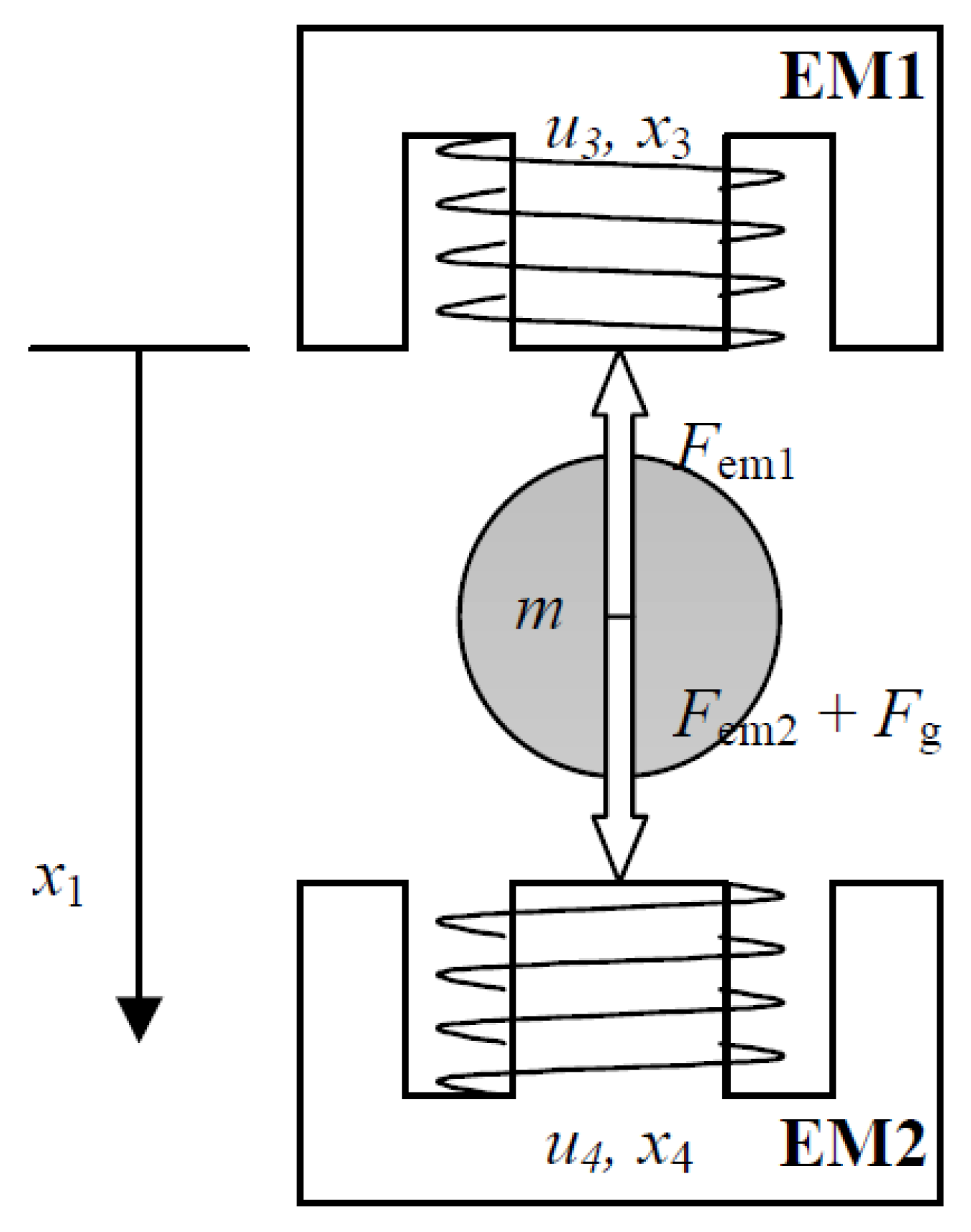
As part of the study, the model of the laboratory magnetic levitation system in the form of a metal ball suspended between two electromagnets is investigated. The device, presented in Figure 1, is described by the following nonlinear differential equations [19]
where
The utilized parameters of the model are:
- system constants
- —0.0243 [A],
- — [H],
- — [m],
- — [m·s],
- — [m],
- — [A],
- —attraction force of the upper electromagnet [N],
- —attraction force of the lower electromagnet [N],
- —force of gravity [N],
- g—acceleration of gravity—9.81 [],
- m—mass of ball—0.0571 [kg],
- —electric voltage of the upper coil—<>, [V],
- —electric voltage of the lower coil—<> [V],
- —distance from the upper magnet to ball minus its diameter—defined by user [m],
- —distance from the upper magnet to ball—<> [m],
- —linear speed of the ball— [],
- —coil current of the upper electromagnet—<>, [A],
- —coil current of the lower electromagnet—<> [A].
Other system’s peculiarities can be found in the Inteco user’s manual [19].
Figure 1.
Examined magnetic levitation system [19].
Figure 1.
Examined magnetic levitation system [19].

3. Performance Indices
Before going into the main goal of this paper covering the different types of control strategies, in this section, the crucial performance indices are tackled. The tabulated below indices are helpful during comparative case studies of proposed control algorithms. In the paper, the following criteria are observed [20,21]:
- ISE (Integral of Squared Error):
- MOE (Minimum of Absolute Energy):
- RT (Regulation Time): the time index, which determines how long it takes for the output signal to reach an area within ±5% around the reference value. For this criterion, the control time was investigated in appropriate steady states.
Note that the discussion involving the aforementioned indices is effectively presented in Section 7. On the other hand, in the next sections, the details of the utilized control schemes are presented.
4. Classical PD Controller
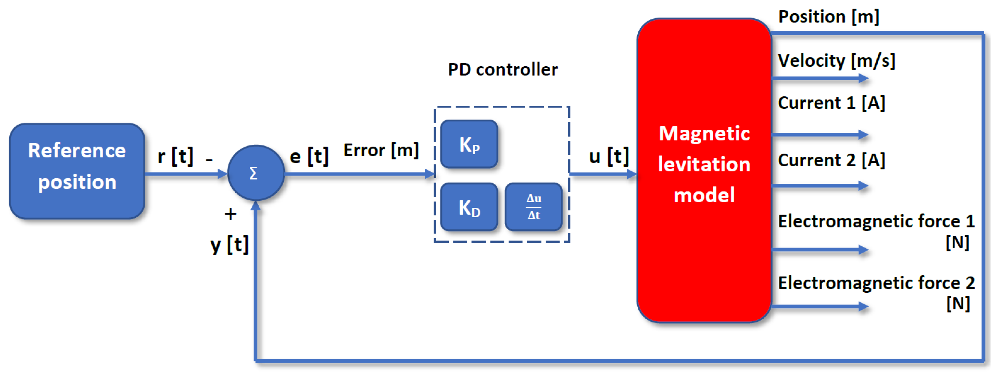
The considered object of magnetic levitation constitutes a laboratory device; it works based on a dedicated proportional–differential PD controller used for both the real system and its model. Due to the nature of the plant operation in the EMS technology (falling ball in an electromagnetic field), it was assumed that the feedback value entering the summation node is positive, while the reference signal is negative. This approach is attractive in order to obtain the positive values of proportional and differential elements [19,20]. It should be emphasized that the levitation process device is related to the multivariable plant (Figure 2); thus, the position of the ball is assumed as the operating point. As we will see, the presented PD controller has some drawbacks, so the optimal control structures are still required.
Simulation Studies
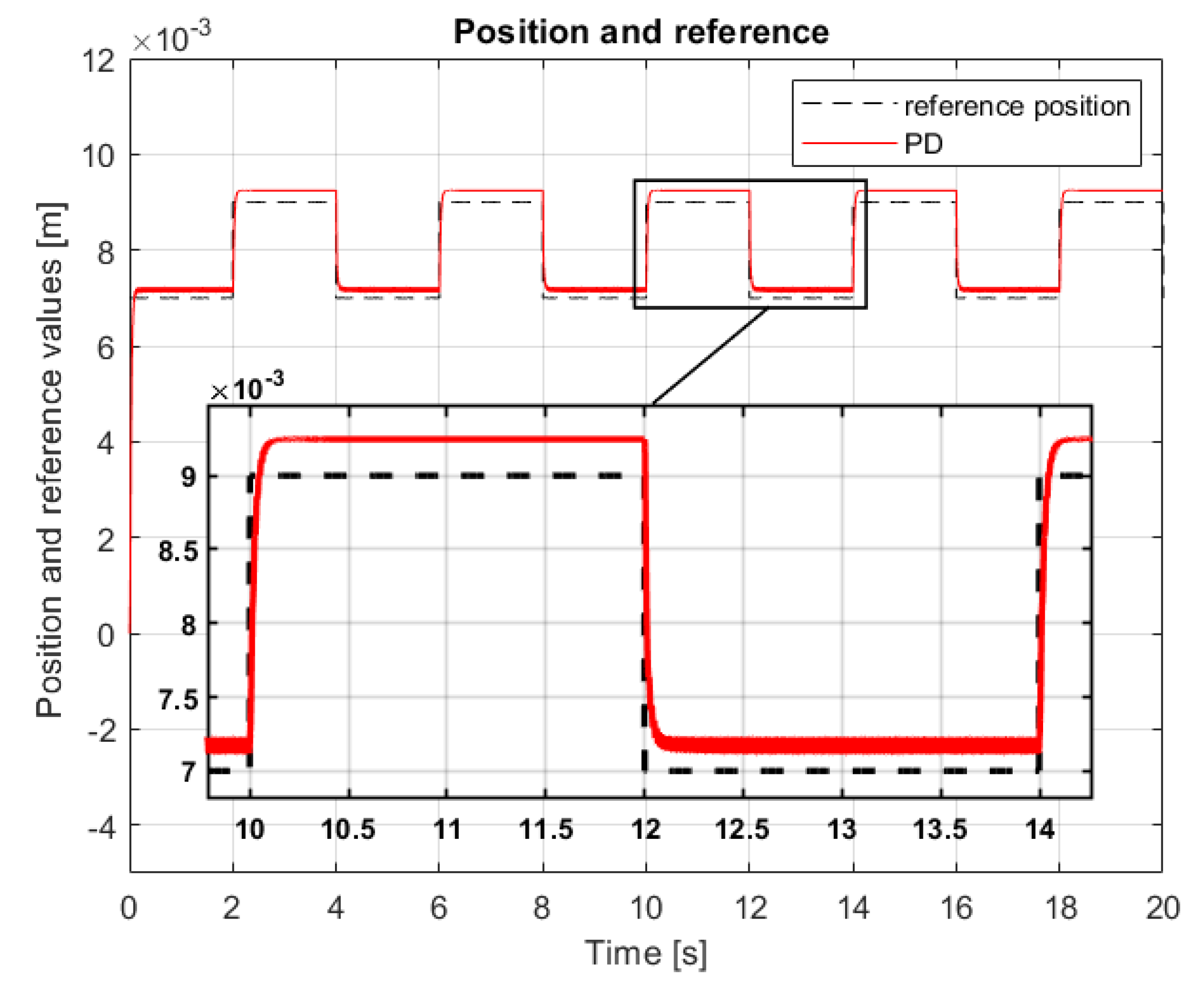
In this part, the PD-originated results derived from the scheme of Figure 2 are discussed. The reference signal is related to the position of the levitating ball located in the following meter scale range = <>, calculated from the upper electromagnetic base—the position is changing in every 2 s. After applying the engineering method, we obtain the crucial parameters = 1500 and = 40 along with the time domain plots depicted in Figure 3. Although the dynamic behavior of the closed-loop control system is rather impressive—a time needed to obtain the reference values is equal to 200 ms, the steady-state error is certainly occurred. According to the factory device without an integral action, the reference error covers the range = <> in the meter scale.
The details of the control actions are shown in Section 7. On the other hand, the next section presents the own improved approach to control of the magnetic levitation process.
5. Hybrid Fuzzy Logic PID Controller
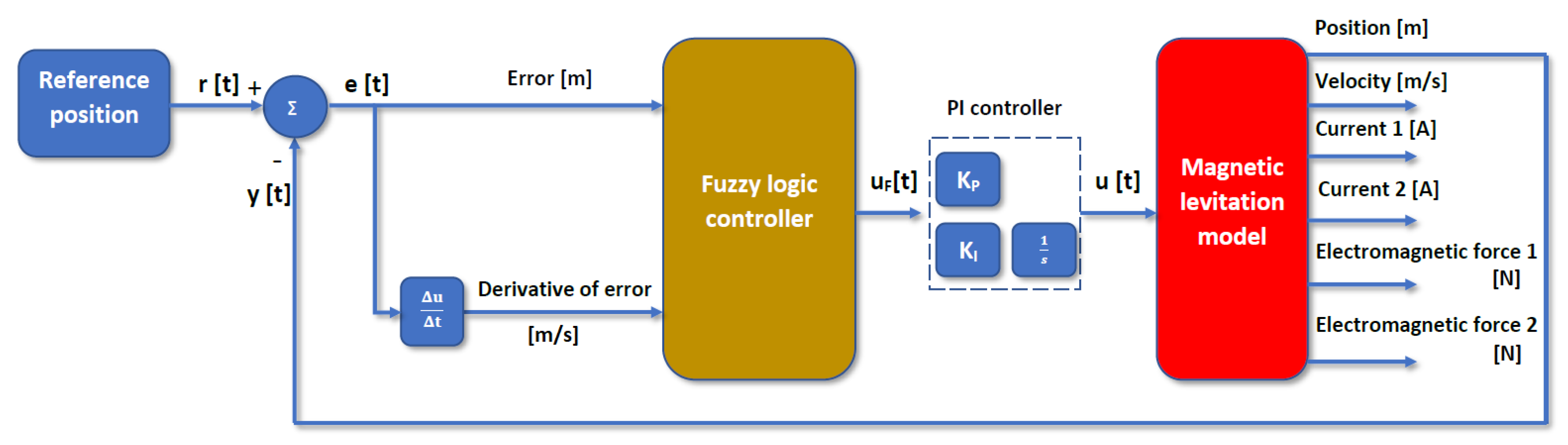
The first step in the search for an appropriate control scheme dedicated to the said magnetic levitation process is an application of a original solution combing the fuzzy logic paradigm with the classical regulator. As a result, the PD-type fuzzy structure has been connected with the PI-oriented plant to finally obtain an improved closed-loop control scheme with quite good dynamics having zero steady-state error. The PID output signal has certainly been given to the upper electromagnet in the form of supply voltage (see Figure 4).
Note that the aforementioned fuzzy logic PD controller is derived from the Mamdani model. It comprises two input signals (error and derivative of error) and one control output calculated according to the following expression
The examined signals have been described in the linguistic domain as follows: —control error, —error derivative, and —control output, all covered by the Table 1 in the context of their membership.
During selection of the linguistic variables, the different membership functions have been utilized. It has been assumed that two functions, i.e., so-called triangular and trapezoidal, would describe two input signals. The reason is that discussed functions are quite easy under the implementation process and their parameters are intuitive as well as simple to interpret. However, it should also be noted that these functions are sharp—the property can change their values and derivatives rapidly. Indeed, as a consequence, the continuous derivative behavior is omitted here [22,23]. The output-related fuzzy sets have been subjected to the defuzzification process according to the Gaussian distribution as follows [23]
where symbol c describes the center of function, whereas symbol denotes the function width. The performed fuzzy logic rules, derived from the membership functions (see Table 1), have been arranged in the form of a MacVicar-Whelan matrix (see Table 2).
As has been mentioned before, the discussed approach allows us to treat the system as the so-called “black box” without any knowledge covering its physical phenomena strictly providing to determine the model of the object. Thus, the presented methodology is universal for the other EMS-originated control purpose.
It should strongly be emphasized that the output set of membership functions has been calculated twofold. The first case has been derived from the expert experience, while the second one has been associated with the genetic algorithm application. Indeed, in the former approach, the expert knowledge has formed the shapes of said functions in contrary to the last method, where the advance genetic algorithm procedure was looking for some optimum related to the assumed performance indices.
The results of the conducted simulation study are shown in the next section.
Simulation Studies
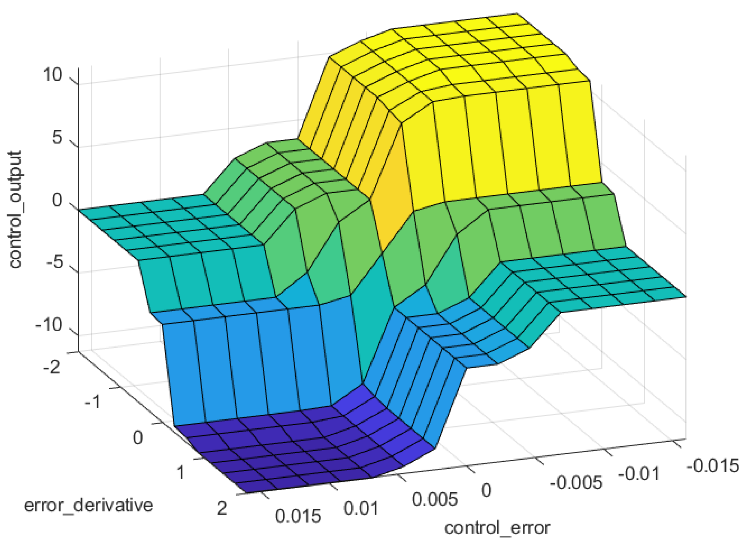
Observe that performed rules (see the MacVicar-Whelan matrix) allow us to obtain the proper surface of the fuzzy logic controller (see Figure 5). Accordingly, the entire PID scheme has been included in the predefined closed-loop control system as shown in Figure 4. After that, the dynamic behavior of the discussed plant has been analyzed using the same paradigm as in the PD case.
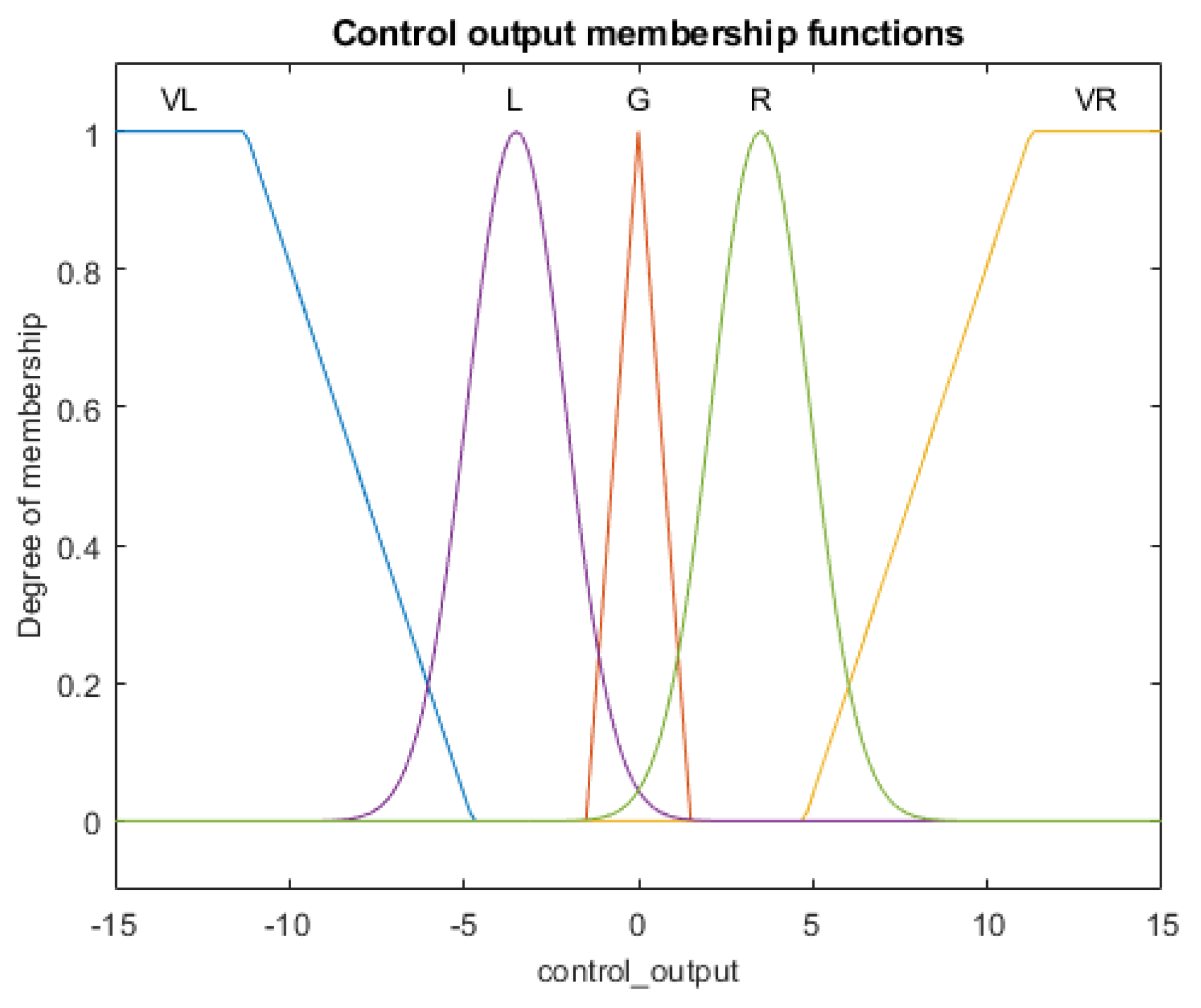
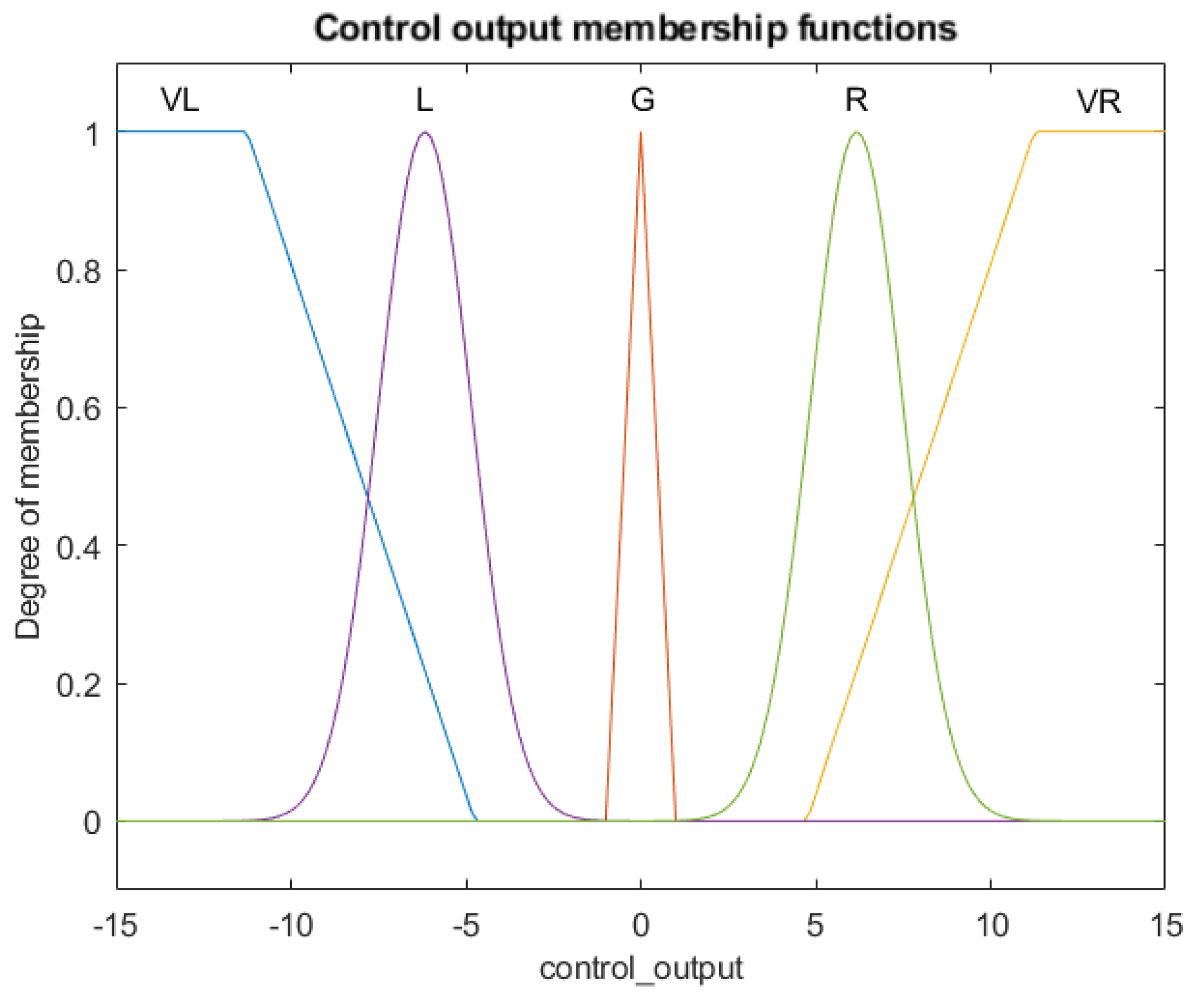
Since the output sets have played an important role during design of the overall control structure, especially in the terms of selection of membership functions, they have been strictly analyzed, as these form the proper input variable runs. For that reason, same as before, two approaches have been reported. The first method employing the expert knowledge with arbitrarily assumed membership functions (see Figure 6) and the second one involving the parameters derived from the genetic algorithm procedure (see Figure 7). For the space limitation reason as well as the similarity of the characteristics in the time domain, the presented results in this section concern exclusively the former expert solution as shown in Figure 8. The slight difference can only be indicated throughout the examined performance indices of Section 7.
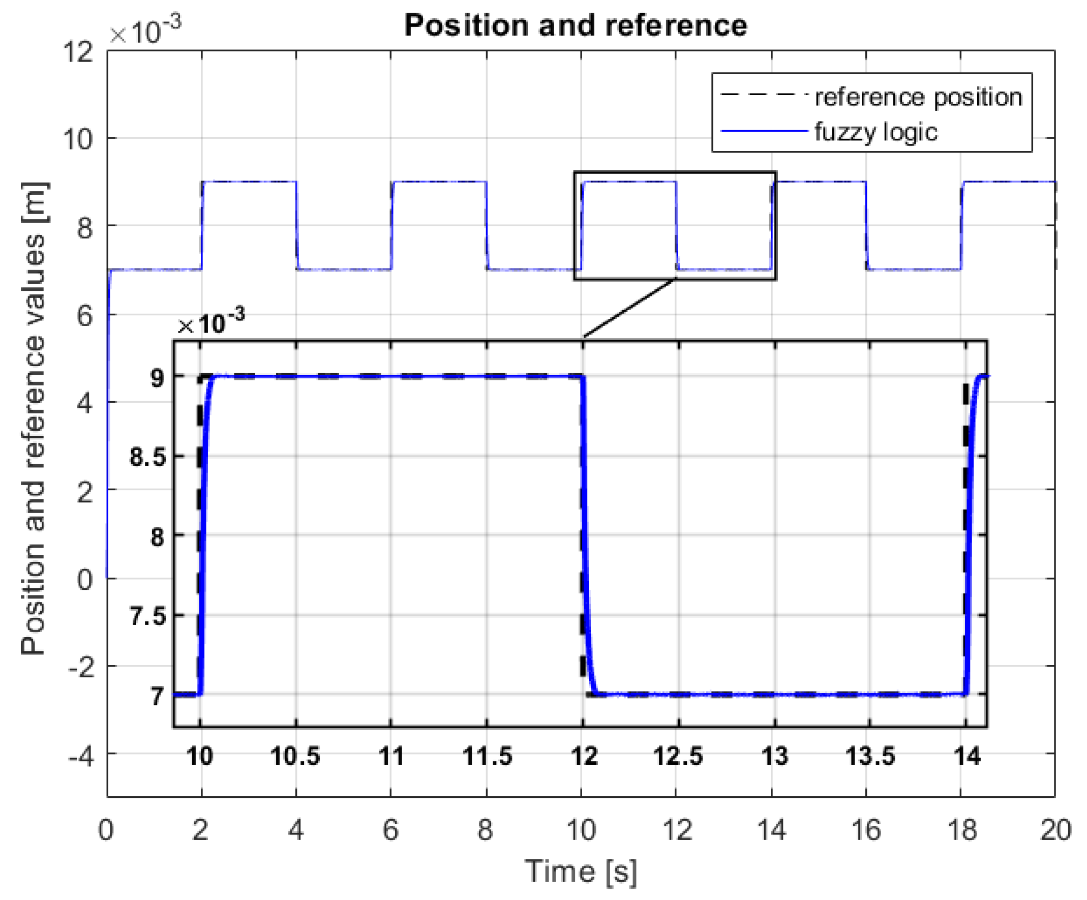
Furthermore, as a result of application of combined PID algorithm (fuzzy logic PD with classical PI), the steady-state error has been reduced to zero and the control time has been shortened as well (see Figure 8). Observe, that there is a possibility to obtain the discussed zero-error by the fuzzy logic controller exclusively. However, such instance is connected with the action of proper forming of utilized rules, which is worth extensive research effort in the nearest future.
In the next section, another neural network approach is proposed.
6. Neural Network Control
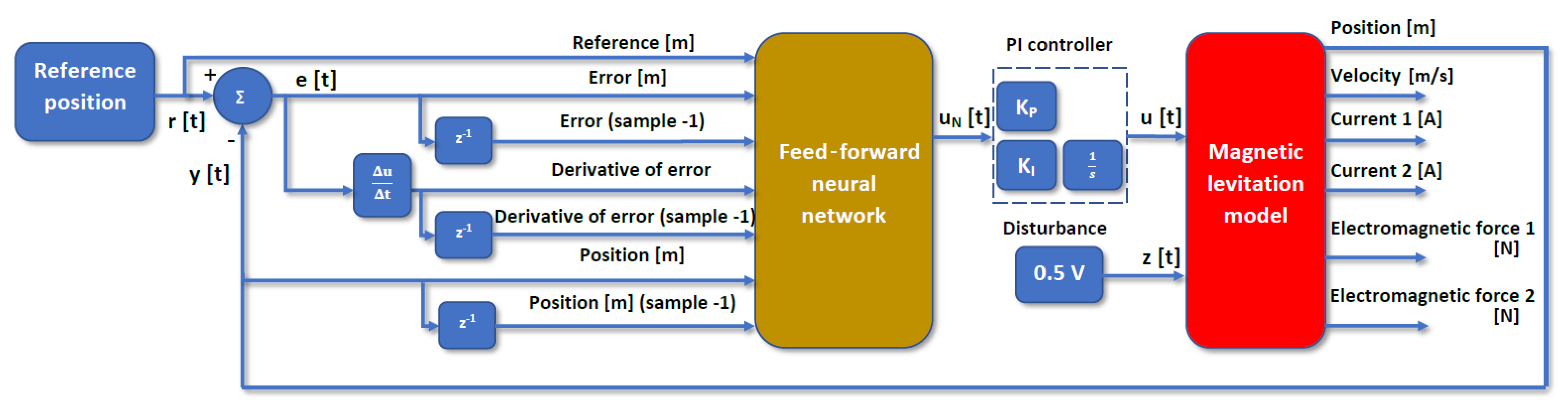
In this section, near to the earlier presented solutions, the advanced neural network approach is investigated. Therefore, in order to approximate the nonlinear continuous-time function according to the theorem of Kolmogorov and Cybenko, the neural network has been examined, which consists of the nonlinear neurons in the first layer and linear neurons in the second one [24,25]. Naturally, a number of nonlinear neurons should be proper in the context of providing an accurate behavior of the objective neural network scheme. Regarding the assumed structure of the control system as in the Figure 9, the simulation study has involved two network layers with one nonlinear hidden layer and single linear output layer. A number of neurons located in the hidden layer have been calculated according to the following formula
where k denotes the number of plant’s inputs and m provides the number of neurons with nonlinear activation function. Although the m should be equal to 14, an additional simulation studies have indicated that (better behavior covering a generalization). Moreover, the supplementary PI controller has been utilized, which properly reinforces and integrates the output signal of the artificial neural network. Thus, the control signal is obtained (see Figure 9). In the next sections, the structure of discussed network is described through the more detailed way.
6.1. The Structure of the Proposed Neural Network
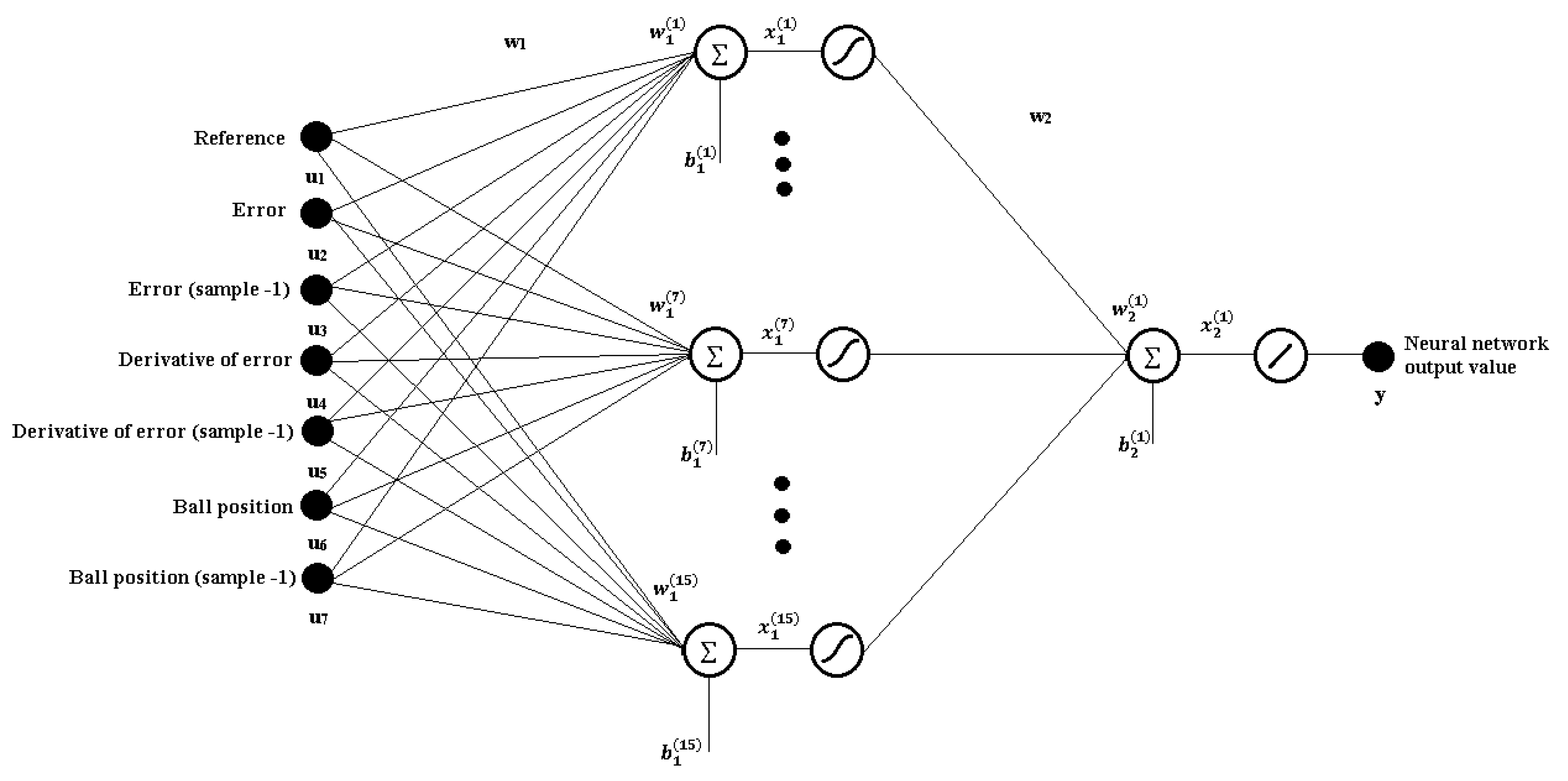
During the study, it was assumed that the first hidden layer will consist of 15 nonlinear neurons having tangensoidal activation function (tansig(.)) as follows [26,27]
The reason is that the said function provides better results and a wider range of possibilities due to the description in the = <> range, in contrast to the sigmoidal form, which takes only non-negative results. The second part of the feed-forward neural network involves a single layer containing a neuron with a linear activation function (purelin(.)). Such structure is strictly derived from the single output of the system. It should be noted that in the case of the designed neural network, the linear part serves the effect of summing up the nonlinear activation functions of neurons located in the preceding layer. Thus, the process of approximation of the nonlinear function, which is the control signal, has satisfactorily been conducted.
Taking into account the above considerations, the output of the feed-forward neural network is described by the simplified formula [28]
where and denote the gain sets of the first and second layer, respectively. The symbols and define the threshold values for respective nonlinear and linear layers, whereas is assumed activation function of the first layer of the neural network. Naturally, the expression (9) can be expanded in the following manner
The graphical scheme of Equation (10) is presented through Figure 10. It should additionally be noted here that feed-forward neural networks are noninertial systems. This means that the values of the network outputs become fixed when signals are applied to the network inputs. This property is desirable for the considered process because the maximum speed of the regulation system should be maintained. The proposed structure of the neural network turned out to be sufficient to design of a properly functioning regulator of the magnetic levitation plant. This fact is confirmed by simulation results shown later in this chapter. On the other hand, the concept used during the task of network training is presented below.
6.2. Supervised Learning of the Neural Network
In order to obtain the appropriate values of the weighting factors of the nonlinear neural network, the reference data derived from the fuzzy logic mechanism have been applied in the learning process. As part of the training of the supervised network, the mean-square-error-originated performance index has been minimized. The aforementioned norm is expressed as follows
where t denotes the reference value and y constitutes the output of the system. The symbol k provides the number of considered elements. The process of optimal training has consisted in minimizing the aforementioned index according to the weighting matrices (of both network layers) and threshold values in regard to the subsequent formula [28]
In the learning process, the input set has been used, which has employed the n = 7 patterns u each of them having k = 20,000 elements as well as the output set arranging the l = 1 pattern t with k = 20,000 elements. The above statements can be described in the following manner covering
and
The sizes of the training sets in the context of input and output variables clearly resulted from the adopted neural network and the nature of the investigated model of the entire object.
6.3. Artificial Neural Network Training Procedure
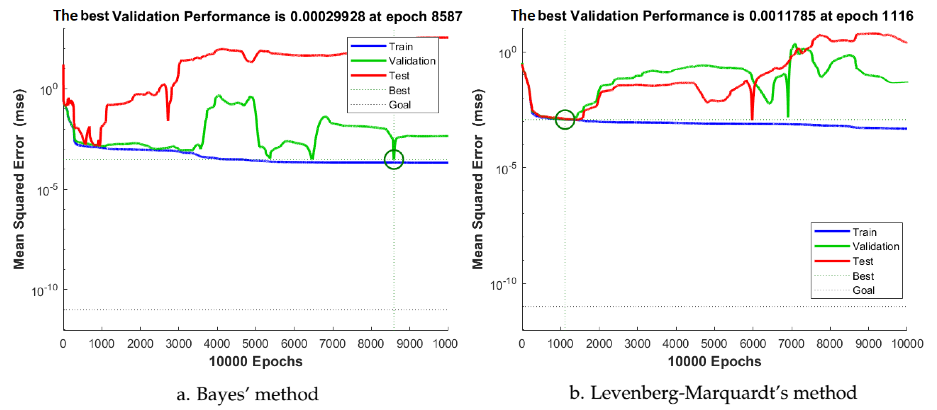
At the beginning of this section, it should be emphasized that two gradient-related methods have been compared under research studies, i.e., Levenberg–Marquardt (trainlm(.)) and Bayes (trainbr(.)) approaches—two offered by the MATLAB environment. In the former solution, the approximated Hessian matrix of the network error function is calculated using its gradient and some regularization factor. One of the main advantages of the discussed method is a convergence. Moreover, in the case of this approach, the limitation of the classical Newton’s algorithm does not occur. Therefore, it is one of the best methods of the small and medium neural networks training [29,30]. On the other hand, the Bayes approach can train any network that meets the following conditions: weight and input data as well as the transfer function are differentiable functions [29,31,32].
The training task respecting the aforementioned tools allows us to obtain much better generalization properties using the Bayes method. For this approach, the least value of the assumed performance index (see Formula (11)) was , while under the Levenberg–Marquardt algorithm, we got . Therefore, the Bayes’ method has been chosen for the training purpose. Figure 11 shows the training process of the neural network along with the validation task for both kinds of algorithms. The differences of the two approaches are clearly visible.
On the other hand, the following section shows the simulation studies for the trained network.
6.4. Simulation Studies
In order to present the validity of resulted control scheme, an additional disturbance has been implemented. The reason is that we would like to know whether the network is overtrained—in such a case, the generalization behavior could be lost. As the disturbance , the DC voltage equal to 0.5 V has been given on the lower electromagnet (see Figure 9).
Figure 12 shows the big potential of the discussed approach. The more precise control scheme allows us to obtain a reference value after approximately 110 ms.
In the next section, the comparison of the analyzed control strategies is finally examined.
7. The Discussion of Obtained Results
As part of the comparative analysis, the simulation tests were carried out for the proposed different types of control schemes. The ball position signal from the range = <> has been changed every 2.5 s; thus, the run has been treated as the setpoint value. The received results of the considered performance indices are summarized in Table 3. After considering the outcomes, it can be stated that the control methods in the field of artificial intelligence have coped much better in contrast to the classical PD regulator. In the PD application case, the steady-state error, calculated according to the discussed performance indices, has been greatest along with the longest regulation time. However, it was the most energy-saving control process. Moreover, it can be observed from the obtained results that the best quality of regulation was provided by the neural network, although it was the most energy-consuming strategy. On the other hand, for the fuzzy logic phenomenon, the performance indices were slightly worse but still better than these derived from the dedicated solution covering the PD controller. Therefore, for the two considered approaches (selection of the membership functions using: (1) the expert method and (2) the genetic algorithm), the genetic algorithm has guaranteed a faster and more accurate regulation process in opposite to the expert method. Unfortunately, the energy of the control runs was much higher in the former case.
Thus, the proposed modern AI control techniques can be treated as the effective ones in some engineering sense.
8. Conclusions
In this paper, the original control schemes dedicate to the magnetic levitation system of the EMS-type are provided. The hybrid PID controller based on the fuzzy logic mechanism and the feed-forward neural network control procedure have certainly been proposed. It turned out that the approaches based on the computational intelligence are quite better than the classical solution covering the PD-related control method. The application of neural network and fuzzy logic paradigms provides robust control schemes in the context of accuracy and speed. However, the modern AI techniques, which do not involve an analytical model of the analyzed plant, are more energy-consuming solutions—this fact has effectively been confirmed by the conducted investigation. Having the experience derived from the simulation studies, the crucial open problem should immediately be formulated. It would be interesting to verify the entire proposed methodology in terms of other performance indices containing the energy of the control input runs. This challenge is worth further intense investigations.
Author Contributions
Conceptualization, D.P. and K.S.; methodology, D.P., K.S. and P.M.; software, D.P. and K.S.; validation, D.P., K.S., W.P.H. and P.M.; formal analysis, W.P.H. and P.M.; investigation, D.P. and K.S.; writing—original draft preparation, D.P., K.S., W.P.H. and P.M.; writing—review and editing, W.P.H. and P.M.; visualization, D.P. and K.S.; supervision, P.M. All authors have read and agreed to the published version of the manuscript.
Funding
This research received no external funding.
Institutional Review Board Statement
Not applicable.
Informed Consent Statement
Not applicable.
Data Availability Statement
Data are contained within the article.
Conflicts of Interest
The authors declare no conflict of interest.
References
- Majewski, P.; Hunek, W.P.; Krok, M. Perfect Control for Continuous-Time LTI State-Space Systems: The Nonzero Reference Case Study. IEEE Access 2021, 9, 82848–82856. [Google Scholar] [CrossRef]
- Krok, M.; Hunek, W.P.; Feliks, T. Switching Perfect Control Algorithm. Symmetry 2020, 12, 816. [Google Scholar] [CrossRef]
- Chen, J.; Liu, Z.; Wang, H.; N’unez, A.; Han, Z. Automatic defect detection of fasteners on the catenary support device using deep convolutional neural network. IEEE Trans. Instrum. Meas. 2017, 67, 257–269. [Google Scholar] [CrossRef] [Green Version]
- Teban, T.A.; Precup, R.E.; Lunca, E.C.; Albu, A.; Bojan-Dragos, C.A.; Petriu, E.M. Recurrent Neural Network Models for Myoelectricbased Control of a Prosthetic Hand. In Proceedings of the 2018 22nd International Conference on System Theory, Control and Computing (ICSTCC), Sinaia, Romania, 10–12 October 2018; pp. 603–608. [Google Scholar] [CrossRef]
- Nguyen, P.D.; Nguyen, N.H.; Ali, A.; Norazak, S. A New Fuzzy PID Control System Based on Fuzzy PID Controller and Fuzzy Control Process. Int. J. Fuzzy Syst. 2020, 22, 2163–2187. [Google Scholar] [CrossRef]
- Wang, D.; Wang, M.; Li, Y. Genetic and Fuzzy Fusion Algorithm for Coal-feeding Optimal Control of Coal-fired Power Plant. In Proceedings of the 2020 International Symposium on Computer, Consumer and Control (IS3C), Taichung, Taiwan, 13–16 November 2020; pp. 500–503. [Google Scholar] [CrossRef]
- Li, A.L.; Wu, H.T. The solid tire sulphation control system based on PLC and Fuzzy adaptive PID control algorithm. In Proceedings of the 2011 International Conference on Electric Information and Control Engineering, Wuhan, China, 25–27 March 2011; pp. 3740–3743. [Google Scholar] [CrossRef]
- Cho, H.W.; Yu, J.S.; Jang, S.M.; Kim, C.H.; Lee, J.M.; Han, H.S. Equivalent Magnetic Circuit Based Levitation Force Computation of Controlled Permanent Magnet Levitation System. IEEE Trans. Magn. 2012, 48, 4038–4041. [Google Scholar] [CrossRef]
- Chamraz, Š.; Huba, M.; Žáková, K. Stabilization of the Magnetic Levitation System. Appl. Sci. 2021, 11, 369. [Google Scholar] [CrossRef]
- Kim, C.H.; Lim, J.; Lee, J.M.; Han, H.S.; Park, D.Y. Levitation control design of super-speed Maglev trains. In Proceedings of the 2014 World Automation Congress (WAC), Waikoloa, HI, USA, 3–7 August 2014; pp. 729–734. [Google Scholar] [CrossRef]
- Barambones, O.; Alkorta, P.; Garrido, A.; Garrido, I.; De la Sen, M.; Maseda, F.; Martija, I. A Neural Networks based variable structure control scheme for induction motors. In Proceedings of the Conference of the Intelligent Systems and Control, Kaohsiung, Taiwan, 26–28 November 2008; Volume 633, p. 53. [Google Scholar]
- Dettori, S.; Iannino, V.; Colla, V.; Signorini, A. An adaptive Fuzzy logic-based approach to PID control of steam turbines in solar applications. Appl. Energy 2018, 227, 655–664. [Google Scholar] [CrossRef]
- Taghdisi, M.; Balochian, S. Maximum Power Point Tracking of Variable-Speed Wind Turbines Using Self-Tuning Fuzzy PID. Technol. Econ. Smart Grids Sustain. Energy 2020, 5, 8. [Google Scholar] [CrossRef]
- Jin, L.; Zhang, R.; Tang, B.; Guo, H. A Fuzzy-PID Scheme for Low Speed Control of a Vehicle While Going on a Downhill Road. Energies 2020, 13, 2795. [Google Scholar] [CrossRef]
- Wang, Z.; Yi, G.; Zhang, S. An Improved Fuzzy PID Control Method Considering Hydrogen Fuel Cell Voltage-Output Characteristics for a Hydrogen Vehicle Power System. Energies 2021, 14, 6140. [Google Scholar] [CrossRef]
- Morán-Durán, A.; Martínez-Sibaja, A.; Rodríguez-Jarquin, J.P.; Posada-Gómez, R.; González, O.S. PEM Fuel Cell Voltage Neural Control Based on Hydrogen Pressure Regulation. Processes 2019, 7, 434. [Google Scholar] [CrossRef] [Green Version]
- Lalik, K.; Wątorek, F. Predictive Maintenance Neural Control Algorithm for Defect Detection of the Power Plants Rotating Machines Using Augmented Reality Goggles. Energies 2021, 14, 7632. [Google Scholar] [CrossRef]
- Ren, Y.; Zhao, Z.; Zhang, C.; Yang, Q.; Hong, K.S. Adaptive Neural-Network Boundary Control for a Flexible Manipulator With Input Constraints and Model Uncertainties. IEEE Trans. Cybern. 2021, 51, 4796–4807. [Google Scholar] [CrossRef]
- INTECO. Magnetic Levitation System 2EM, User’s Manual. Available online: https://pdfslide.tips/documents/magnetic-levitation-system-2em.html (accessed on 1 January 2022).
- Kaczorek, T.; Dzieliński, A.; Dąbrowski, W.; Łopatka, R. Fundamentals of Control Theory; WNT: Warsaw, Poland, 2016. (In Polish) [Google Scholar]
- Özdemir, M.T.; Öztürk, D. Comparative performance analysis of optimal PID parameters tuning based on the optics inspired optimization methods for automatic generation control. Energies 2017, 10, 2134. [Google Scholar] [CrossRef] [Green Version]
- Piegat, A. Fuzzy Modeling and Control; Physica: Heidelberg, Germany, 2013; Volume 69. [Google Scholar]
- Jang, J.S.R.; Sun, C.T.; Mizutani, E. Neuro-fuzzy and soft computing-a computational approach to learning and machine intelligence. IEEE Trans. Autom. Control 1997, 42, 1482–1484. [Google Scholar] [CrossRef]
- Michalkiewicz, J. Modified Kolmogorov’s theorem. Math. Appl. 2009, 37, 23–38. [Google Scholar] [CrossRef]
- Bielecki, A. Mathematical principles of artificial neural networks. Math. Appl. 2003, 31, 25–55. [Google Scholar] [CrossRef]
- Beale, M.H.; Hagan, M.T.; Demuth, H.B. Neural network toolbox. In User’s Guid; MathWorks: Natick, MA, USA, 2017; Volume 2. [Google Scholar]
- Suzuki, K. Artificial Neural Networks: Architectures and Applications; Intech: Singapore, 2013. [Google Scholar]
- Kriegeskorte, N.; Golan, T. Neural network models and deep learning. Curr. Biol. 2019, 29, R231–R236. [Google Scholar] [CrossRef] [PubMed]
- Kayri, M. Predictive abilities of bayesian regularization and Levenberg–Marquardt algorithms in artificial neural networks: A comparative empirical study on social data. Math. Comput. Appl. 2016, 21, 20. [Google Scholar] [CrossRef]
- Rutkowski, L. Methods and Techniques of Artificial Intelligence; PWN: Warszawa, Poland, 2005. (In Polish) [Google Scholar]
- MacKay, D.J. Bayesian interpolation. Neural Comput. 1992, 4, 415–447. [Google Scholar] [CrossRef]
- Foresee, F.D.; Hagan, M.T. Gauss-Newton approximation to Bayesian learning. In Proceedings of the International Conference on Neural Networks (ICNN’97), Houston, TX, USA, 12 June 1997; Volume 3, pp. 1930–1935. [Google Scholar]
Figure 2.
Magnetic levitation system with PD controller.

Figure 3.
The system response—the PD controller case.

Figure 4.
Diagram of magnetic levitation system involving a hybrid fuzzy logic PID controller.

Figure 5.
The control surface of the fuzzy logic controller.

Figure 6.
The membership functions of the control output set—the expert method.

Figure 7.
The membership functions of the control output set—the genetic algorithm method.

Figure 8.
The system response—the hybrid PID controller case.

Figure 9.
The structure of the neural network control system.

Figure 10.
The structure of the original neural network.

Figure 11.
The observation of obtained results.

Figure 12.
The system response—the neural network controller case.


Table 1.
The input and output membership functions.
| VN—Very Negative | FD—Fast decreasing | VL—Very Low |
| N—Negative | D—Decreasing | L—Lower |
| G—Good | G—Good | G—Good |
| P—Positive | I—Increasing | R—Raise |
| VP—Very Positive | FI—Fast Increasing | VR—Very Raise |
Table 2.
The rules of the fuzzy logic controller.
| FD | D | G | I | FI | |
|---|---|---|---|---|---|
| VN | VR | VR | R | R | G |
| N | VR | VR | R | G | L |
| G | R | R | G | L | L |
| P | R | G | L | VL | VL |
| VP | G | L | L | VL | VL |
Table 3.
The results of the performance indices.
Publisher’s Note: MDPI stays neutral with regard to jurisdictional claims in published maps and institutional affiliations. |
© 2022 by the authors. Licensee MDPI, Basel, Switzerland. This article is an open access article distributed under the terms and conditions of the Creative Commons Attribution (CC BY) license (https://creativecommons.org/licenses/by/4.0/).
Share and Cite
MDPI and ACS Style
Majewski, P.; Pawuś, D.; Szurpicki, K.; Hunek, W.P. Toward Optimal Control of a Multivariable Magnetic Levitation System. Appl. Sci. 2022, 12, 674. https://0-doi-org.brum.beds.ac.uk/10.3390/app12020674
AMA Style
Majewski P, Pawuś D, Szurpicki K, Hunek WP. Toward Optimal Control of a Multivariable Magnetic Levitation System. Applied Sciences. 2022; 12(2):674. https://0-doi-org.brum.beds.ac.uk/10.3390/app12020674
Chicago/Turabian StyleMajewski, Paweł, Dawid Pawuś, Krzysztof Szurpicki, and Wojciech P. Hunek. 2022. "Toward Optimal Control of a Multivariable Magnetic Levitation System" Applied Sciences 12, no. 2: 674. https://0-doi-org.brum.beds.ac.uk/10.3390/app12020674
Note that from the first issue of 2016, this journal uses article numbers instead of page numbers. See further details here.