Predictive Control for Small Unmanned Ground Vehicles via a Multi-Dimensional Taylor Network

Abstract

Tracking control of Small Unmanned Ground Vehicles (SUGVs) is easily affected by the nonlinearity and time-varying characteristics. An improved predictive control scheme based on the multi-dimensional Taylor network (MTN) is proposed for tracking control of SUGVs. First, a MTN model is used as a predictive model to construct a SUGV model and back propagation (BP) is taken as its learning algorithm. Second, the predictive control law is designed and the traditional objective function is improved to obtain a predictive objective function with a differential term. The optimal control quantity is given in real time through iterative optimization. Meanwhile, the stability of the closed-loop system is proved by the Lyapunov stability theorem. Finally, a tracking control experiment on the SUGV model is used to verify the effectiveness of the proposed scheme. For comparison, traditional MTN and Radial Basis Function (RBF) predictive control schemes are introduced. Moreover, a noise disturbance is considered. Experimental results show that the proposed scheme is effective, which ensures that the vehicle can quickly and accurately track the desired yaw velocity signal with good real-time, robustness, and convergence performance, and is superior to other comparison schemes.

1. Introduction

With the rapid development of artificial intelligence, big data, and data fusion technology, car driving tends to be intelligent and unmanned. Recently, research on Unmanned Ground Vehicles (UGVs) has become a hot topic at home and abroad [1,2,3]. Its core technologies include environmental awareness, vehicle positioning, path planning, and path tracking control [4,5,6,7]. Path tracking control, as a key core issue of unmanned driving technology, has attracted much attention from scholars and it ensures that the car drives on the specified path [7,8,9]. So, research on path tracking control has both theoretical and practical significance.

However, UGV path tracking control is a strongly nonlinear process, which contains time-varying characteristics, uncertainty, etc., and a precise mathematical model is difficult to obtain [10]. As artificial intelligence develops, neural networks can solve the above problem well due to their nonlinear approximation capabilities [11]. For example, a new end-to-end autonomous control method was proposed to simplify the separate modules in the traditional control pipeline into a single neural network [12]. A novel application of the biologically inspired computing paradigm was presented for solving the initial value problem (IVP) of electric circuits based on a nonlinear RL model by exploiting the competency of accurate modeling with a feed forward artificial neural network, the global search efficacy of genetic algorithms, and a rapid local search with sequential quadratic programming [13]. Moreover, predictive control, rooted in industrial engineering, is widely used. Usually, the schemes that combine a neural network model and predictive control are more popular and useful to solve the nonlinear control problem. For example, physics-based recurrent neural network modeling approaches were proposed for a general class of nonlinear dynamic process systems to improve the prediction accuracy by incorporating a priori process knowledge, and the proposed physics-based RNN models were utilized in model predictive controllers [14]. A neural-network-based technique for developing nonlinear dynamic models from empirical data for a model predictive control (MPC) algorithm was presented [15]. However, for the neural networks, they easily reach the local minimum [16].

To solve the issues with nonlinearity, time-varying characteristics, uncertainty, real time, etc. and overcome the problem of neural networks, we adopt a multi-dimensional Taylor network (MTN) and collective solutions. The collective solutions are the most effective as they take advantage of each method. The MTN is an inclusive platform that was first proposed by Zhou and Yan and can be used to describe the nonlinear dynamic characteristics of a system without prior knowledge of the structural information on the system [17,18]. It has been successfully applied to system modeling [19,20] and nonlinear control [21,22,23,24]. In this paper, an improved predictive control scheme based on a MTN is proposed to realize real-time output tracking control of Small Unmanned Ground Vehicles (SUGVs) relative to a given reference path without state feedback. First, the MTN is used as a predictive model to construct the SUGV model and back propagation (BP) is taken as its learning algorithm. Second, a predictive control law is designed to control the SUGV and the traditional objective function is improved to obtain a predictive objective function with a differential term. The optimal control quantity is given in real time through iterative optimization. Meanwhile, the stability of the closed-loop system is proved according to the Lyapunov stability theorem. Based on that, an adjustment method for MTN control law parameters is obtained using the predictive accuracy of the MTN model and the control coefficient. Finally, a tracking control experiment on the SUGV is used to verify the effectiveness of the proposed scheme. For comparison, traditional MTN and RBF predictive control schemes are introduced.

By the above analysis, the main contributions are as follows:

(1)

Although tracking control schemes for SUGVs have been proposed, their schemes have a complex design and are difficult to use in practical applications. Our proposed scheme has a simple structure and is easy to implement.

(2)

As the proposed control scheme adapts online learning, no training process is required. Meanwhile, with its simple structure, the strong approximation capability, and the low complexity of the MTN, desirable real-time performance and speed are guaranteed.

(3)

For the quadratic performance index with the differential term, the differential term can help the system to act in advance, reduce the overshoot, and shorten the adjustment time.

The rest of the paper is arranged as follows. A literature review is presented in Section 2. The materials and methods are given in Section 3. The MTN predictive control scheme with the differential term is summarized in Section 4. Section 5 presents the simulation results and a discussion. Section 6 presents our conclusions.

2. Literature Review

An effective tracking control scheme is critical to UGV path tracking control. Because UGV path tracking control is a strongly nonlinear process, the control methods for previous linear systems seem to be inadequate [25]. At present, the common control methods include adaptive control, sliding mode control, fuzzy control, neural network control, and predictive control [26,27,28,29,30,31,32,33,34,35]. For instance, for formation control of multiple vehicles, the leader–follower error model was built and an adaptive controller was designed to address the uncertain relative distance using the dynamic estimation of the leader–follower distance [26]. A multivariable model reference adaptive control (MRAC) scheme was studied for the automatic carrier-landing control problem of unmanned aerial vehicles with the system dynamics of nonlinearity, multivariable coupling, and parametric uncertainty [27]. A vehicle lateral controller was designed for autonomous vehicles based on higher-order sliding mode control [28]. An automatic steering control strategy for unmanned vehicles based on robust backstepping sliding mode control theory was proposed [29]. For the accuracy and stability of driverless buses, a path-tracking controller based on fuzzy pure pursuit control with a front axle reference (FPPC-FAR) was proposed [30]. An obstacle avoidance strategy consisting of path planning and robust fuzzy output feedback control was proposed for unmanned ground vehicles [31]. A novel adaptive neural network robust lateral motion control method was presented that can maintain the yaw stability of an autonomous vehicle while minimizing the lateral path tracking error at the limits of driving conditions [32]. A learning-based predictive control approach was presented for an autonomous racing car [33]. A nonlinear model predictive control optimization algorithm based on the collocation method was proposed for unmanned vehicle trajectory tracking [34]. A trajectory tracking error-based model was used to design a linear model predictive controller and its control action was combined with feed forward and robust control actions [35].

However, all of the above-mentioned control technologies have their own inherent bottlenecks both in theory and in application. For example, for adaptive control, there are many stability methods to be chosen from when designing the control rate, but most of them require strong assumptions. For fuzzy control, simple fuzzy processing will lead to a reduction in control precision and poor system dynamic quality. For neural network control, the closed-loop system is stable only at a certain point, and the exponential function of neurons will also lead to a large number of computations and poor real-time performance. Sliding mode variable structure control can easily fall into a chattering state, and it also needs to solve for factors such as velocity, inertia, acceleration, and the switching surface when near the sliding mode surface. For predictive control based on a mathematical model, it is difficult to establish an accurate mathematical model, or even to build a model. Therefore, collective solutions were adopted in this study.

The multi-dimensional Taylor network is an inclusive platform and applies to nonlinear control particularly effectively. For example, an adaptive predictive control approach based on the MTN was proposed for the real-time tracking control of single-input single-output nonlinear systems with input time-delay [21]. A control scheme based on the MTN was proposed to achieve the real-time output feedback tracking control of multi-input multi-output non-affine nonlinear time-varying discrete systems relative to the given reference signals with online training [22]. An adaptive control approach based on the MTN was proposed to control nonlinear uncertain time-varying systems with noise disturbances [23]. A predictive control scheme on the basis of the MTN, named MTN predictive compensation control, was proposed for single-input single-output nonlinear systems [24]. However, the above-mentioned studies focus on theoretical research and they do not have an application background. Therefore, an improved predictive control scheme based on the MTN is proposed for the tracking control of SUGVs.

3. Materials and Methods

3.1. System Description of the SUGV

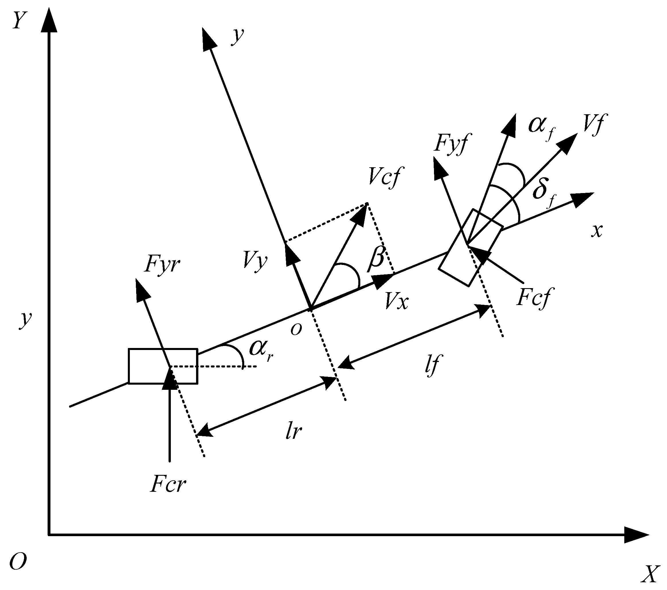
A simplified SUGV model is shown in Figure 1. Two front wheels and two rear wheels are combined into a single front wheel and rear wheel, which are simplified into a two-degrees-of-freedom vehicle model. The following assumptions were made: we ignored the effect of steering and suspension; we kept the vehicle’s longitudinal speed constant and only considered the lateral movement along the y axis and the yaw movement around the z axis; we ignored the effects of horizontal and vertical aerodynamics; and we considered the side characteristics of the tire in the analysis of the tire force [36,37,38].

The XOY coordinate system in Figure 1 is a fixed geodetic coordinate system, and xoy is the structure of the coordinate system, which changes with the movement of the body. The force analysis of the above model along the y axis and around the z axis is obtained.

$$\{\begin{array}{l}M{a}_y=F_{cf}\cos {\delta }_f+F_{cr}\\ I_z\dot{w}=I_f{F}_{cf}\cos {\delta }_f-I_r{F}_{cr}\end{array}$$

(1)

where M is the vehicle’s weight; $I_f$ is the distance between the center of the front axle and the center of mass of the vehicle; $I_r$ is the distance between the center of the rear axle and the center of mass of the vehicle; $I_z$ is the moment of inertia of the vehicle around the z axis; ${\delta }_f$ is the front wheel angle of the vehicle; $w$ is the yaw velocity of the vehicle; and $a_y$ is the accelerated velocity of the vehicle along the y axis based on the xoy coordinate system, which mainly consists of the movement along the y axis and the centripetal acceleration $V_{x}w$. We can obtain:

$$a_y=\ddot{y}+V_{x}w$$

(2)

where $F_{cf}$ and $F_{cr}$ are the lateral force of the tire applied to the front and rear wheels of the vehicle, respectively. From the defined dynamic model, we can see that the side characteristic of the tire is considered in the analysis of the tire force. When the front wheel angle ${\delta }_f$ and the sideslip angle $\beta$ are small, the sideslip characteristic of the tire is in a linear range. So, we can obtain

$$F_{cf}=2C_f{\alpha }_f$$

(3)

$$F_{rf}=2C_r{\alpha }_r$$

(4)

where $C_f$ and $C_r$ are the cornering stiffnesses of the front and rear tires, respectively. Since there are two front and rear wheels, the force is twice that of a single tire. ${\alpha }_f$ and ${\alpha }_r$ are the tire sideslip angle and the angle between the direction of the tire velocity vector and the x axis, respectively. At a small angle, the size of the two angles can be approximately expressed as:

$$\tan {\alpha }_f\approx \theta <V_f,x>=\frac{V_y+l_f\dot{\phi }}{V_x}$$

(5)

$$\tan {\alpha }_r\approx \theta <V_r,x>=\frac{V_y-l_r\dot{\phi }}{V_x}$$

(6)

According to the coordinate system relationship, the side slip angle is $\beta =\tan \beta =\frac{V_y}{V_x}$. From (1)–(6), the differential equation of the vehicle dynamics model is obtained.

$$\{\begin{array}{l}\dot{w}=\frac{l_f^2{C}_f+l_r^2{C}_r}{I_z{v}_x}w-\frac{l_f{C}_f+l_r{C}_r}{I_z}\beta +\frac{l_f{C}_f}{I_z}{\delta }_f\\ \dot{\beta }=(-\frac{l_f{C}_f+l_r{C}_r}{m{v}_x^2}-1)w-\frac{C_f+C_r}{m{v}_x}\beta +\frac{C_f}{m{v}_x}{\delta }_f\end{array}$$

(7)

The control input and output variables of the controlled vehicle are the front wheel steering angle ${\delta }_f$ and the yaw velocity $w$, respectively. According to the vehicle dynamics model, a relation between the output and the input of the controlled system is deduced

$$\ddot{w}(t)=-a_1\dot{w}(t)-a_{2}w(t)+b_1{\dot{\delta }}_f(t)+b_2{\delta }_f(t)$$

(8)

where $a_1=\frac{m(l_f^2{C}_f+l_r^2{C}_r)+I_z(C_f+C_r)}{m{v}_x{I}_z}$, $a_2=\frac{-m{v}_x^2(l_f{C}_f-l_r{C}_r)+C_f{C}_r}{m{v}_x^2{I}_z}$, $b_1=\frac{l_f{C}_f}{I_z}$, $b_2=\frac{C_f{C}_{r}L}{m{v}_x{I}_z}$.

So, the vehicle control system can be described as the following second-order system:

$$\{\begin{array}{l}{\dot{x}}_1=x_2\\ {\dot{x}}_2=F(x_1,x_2,{\dot{\delta }}_f,\gamma (t))+b_0{\delta }_f\\ y=x_1\end{array}$$

(9)

where $x_1=w(t)$, $x_2=\dot{w}(t)$, $b_0=b_2$, $F(x_1,x_2,{\dot{\delta }}_f,\gamma (t))=-a_1\dot{w}(t)-a_{2}w(t)+b_1{\dot{\delta }}_f(t)+\gamma (t)$, and $F(\cdot )$ is defined as a generalized disturbance that includes the modeled and unmodeled parts of the vehicle and an unknown external disturbance.

3.2. Multi-Dimensional Taylor Network Model

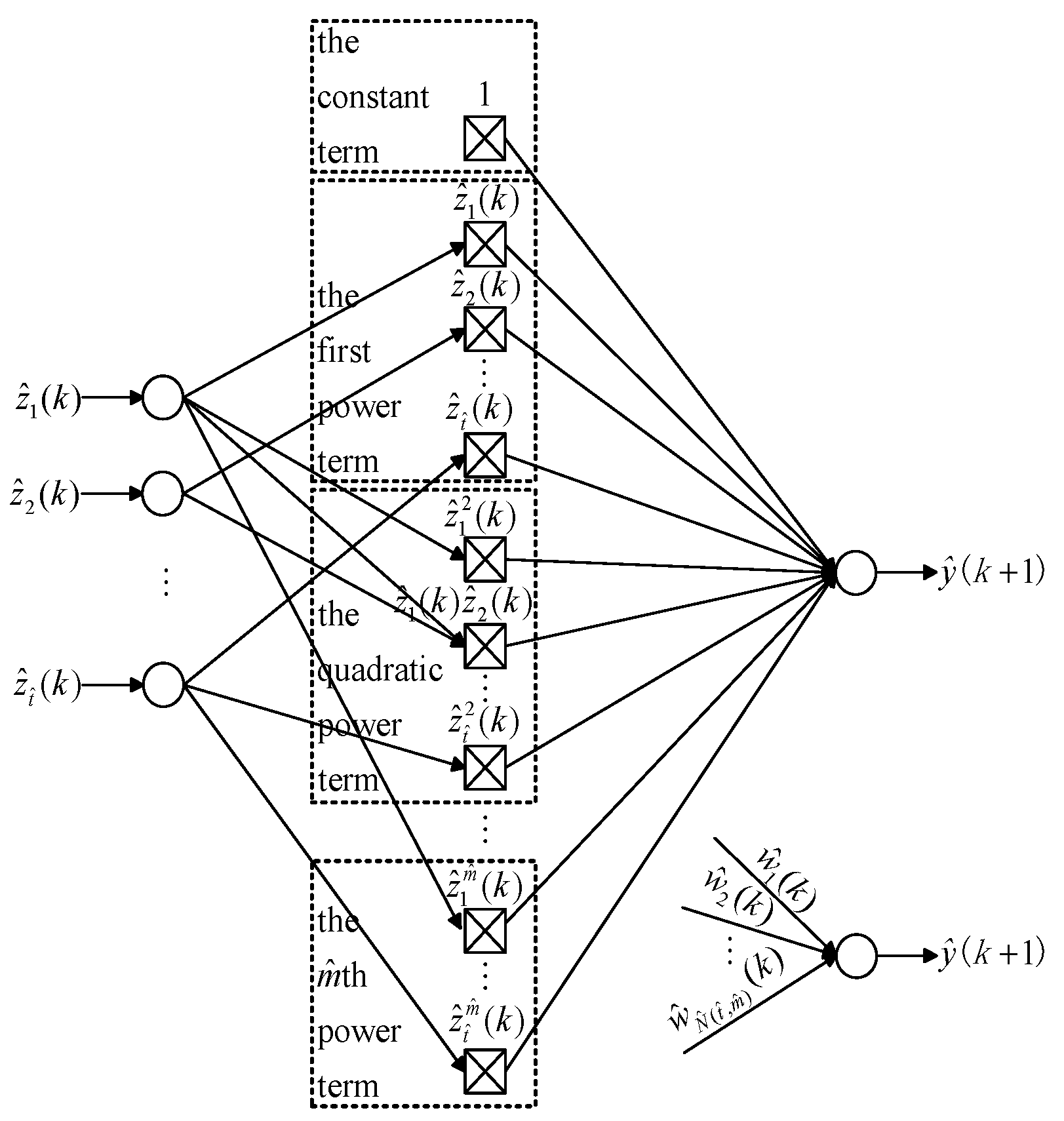
If the function is $\widehat{m}+1$-order differentiable everywhere in the neighborhood at some point, the power series of the eigenfunction expansion at this point is not greater than $\widehat{m}$ power in terms of the principle of the multivariate Taylor formula. Based on the MTN model, as shown in Figure 2, the general dynamic equation of an $\widehat{t}$-dimensional system can be expressed as [17]:

$$\widehat{y}(k+1)={\displaystyle \sum _{\widehat{p}=1}^{\widehat{N}(\widehat{t},\widehat{m})}{\widehat{w}}_{\widehat{p}}(k){\displaystyle \prod _{\widehat{q}=1}^{\widehat{t}}{\widehat{z}}_{\widehat{q}}^{\widehat{\lambda }(\widehat{p},\widehat{q})}(k)}}$$

(10)

In (10), $\widehat{N}(\widehat{t},\widehat{m})$ represents the total number of product items of the $\widehat{t}$-ary function $\widehat{o}[\cdot ]$, which is expanded into the approximate polynomial with $\widehat{m}$ powers; ${\widehat{w}}_{\widehat{p}}(k)$ represents the weight coefficient of the $\widehat{p}$-th product item in the formula; $\widehat{\lambda }(\widehat{p},\widehat{q})$ represents the power of the variable ${\widehat{z}}_{\widehat{q}}(k)$ in the $\widehat{p}$-th product item; and ${\displaystyle \sum _{\widehat{q}=1}^{\widehat{t}}\widehat{\lambda }(\widehat{p},\widehat{q})}\le \widehat{m}$, where $\widehat{p}=1,2,\cdots ,\widehat{N}(\widehat{t},\widehat{m})$.

As can be seen from Figure 2, the MTN is composed of three main layers, including the input layer, the middle layer, and the output layer. Its structure is simple, it contains only addition and multiplication operations, it is equivalent to only one neuron of the neural network, and it has low algorithm complexity, namely real-time performance. Otherwise, the model parameters are obtained through continuous optimization, which has a "self-learning" ability and good robustness.

The MTN model has a powerful approximation capability for nonlinear systems and can approximate any model with sufficient precision as long as $\widehat{N}(\widehat{t},\widehat{m})$ is large enough [21,39].

4. MTN Predictive Control Scheme with the Differential Term

4.1. Scheme of the MTN Predictive Model

4.1.1. MTN Predictive Model

The MTN model is essentially a one-step-ahead predictive model. Therefore, the MTN model can be regarded as a predictive model. We adopt the MTN model as shown in (10).

4.1.2. Learning Algorithm of the MTN Predictive Model

The BP algorithm is used to adjust the weight coefficients of the MTN model [40,41].

Define the cost function as

$$J_{\mathrm{P}}(k)=\frac{1}{2}{e}_{\mathrm{P}}{}^2(k)$$

(11)

where $e_{\mathrm{P}}(k)$ represents the predictive model error and $e_{\mathrm{P}}(k)=y(k)-\widehat{y}(k)$; $y(k)$ is the system output; and $\widehat{y}(k)$ is the predictive model output.

Let

$${\widehat{\mathit{w}}}_{\mathrm{P}}(k)={\left({\widehat{w}}_{\mathrm{P}1}(k),{\widehat{w}}_{\mathrm{P}2}(k),\cdots ,{\widehat{w}}_{\mathrm{P}\widehat{N}(\widehat{t},\widehat{m})}(k)\right)}^{\mathrm{T}}$$

The BP algorithm can be obtained as follows

$${\mathit{w}}_{\mathrm{P}}(k+1)={\mathit{w}}_{\mathrm{P}}(k)+\mu \frac{\partial J_P}{\partial {\mathit{w}}_{\mathrm{P}}(k)}$$

(12)

where $\mu$ is the learning factor and $\mu >0$.

4.2. Design of the Predictive Control Law with the Differential Term

Consider the following quadratic performance index:

$$J_{\mathrm{C}}(k)=\min \left\{\frac{1}{2}{(r(k)-\widehat{y}(k))}^2+\frac{1}{2}\epsilon \Delta u^2(k)\right\}$$

(13)

where $r(k)$ is the reference input, $\widehat{y}(k)$ is the output of the MTN predictive model, $\epsilon$ is the control effort weighting factor, $\Delta u(k)=u(k)-u(k-1)$, and $u(k)$ is the control input.

Denote $\frac{\partial J_{\mathrm{C}}(k)}{\partial u(k)}=0$. We can now obtain the MTN predictive control law:

$$u(k)=u(k-1)+\frac{1}{\epsilon }(r(k)-\widehat{y}(k))\frac{\partial \widehat{y}(k)}{\partial u(k)}$$

(14)

where $u(k)$, $r(k)$, $\widehat{y}(k)$, and $\epsilon$ have the same meaning as in Equation (13).

The differential term is introduced under the traditional quadratic performance index. A differential term can help the system to move in advance, reduce the overshoot, and shorten the adjustment time. Meanwhile, it can reduce the influence of time variation and disturbance factors. The following quadratic performance index with the differential term was adopted:

$$J_{\mathrm{C}}(k)=\min \left\{\frac{1}{2}{e}_{\mathrm{C}}{}^2(k)+\frac{1}{2}\epsilon \Delta u^2(k)+\frac{1}{2}\gamma {\left[e_{\mathrm{C}}(k)-e_{\mathrm{C}}(k-1)\right]}^2\right\}$$

(15)

where $\gamma$ is the differential weighting factor and $\gamma >0$, $e_{\mathrm{C}}(k)=r(k)-\widehat{y}(k)$, $r(k)$, $\widehat{y}(k)$, and $\epsilon$ have the same meaning as in Equation (13).

According to (15),

$$\begin{array}{ll}\frac{\partial J_{\mathrm{C}}(k)}{\partial u(k)}& =e_{\mathrm{C}}(k)\frac{\partial e_{\mathrm{C}}(k)}{\partial u(k)}+\epsilon \Delta u+\gamma \left[e_{\mathrm{C}}(k)-e_{\mathrm{C}}(k-1)\right]\frac{\partial e_{\mathrm{C}}(k)}{\partial u(k)}\\ & =-e_{\mathrm{C}}(k)\frac{\partial \widehat{y}(k)}{\partial u(k)}+\epsilon \Delta u-\gamma \left[e_{\mathrm{C}}(k)-e_{\mathrm{C}}(k-1)\right]\frac{\partial \widehat{y}(k)}{\partial u(k)}\end{array}$$

(16)

where $\epsilon$, $\gamma$, $r(k)$, and $\widehat{y}(k)$ have the same meaning as in (15).

Denote

$$\frac{\partial J_{\mathrm{C}}(k)}{\partial u(k)}=0$$

We can now obtain the MTN predictive control law with the differential term:

$$u(k)=u(k-1)+\frac{1}{\epsilon }{e}_{\mathrm{C}}(k)\frac{\partial \widehat{y}(k)}{\partial u(k)}+\frac{\gamma }{\epsilon }\left[e_{\mathrm{C}}(k)-e_{\mathrm{C}}(k-1)\right]\frac{\partial \widehat{y}(k)}{\partial u(k)}$$

(17)

where $\epsilon$, $\gamma$, $r(k)$, and $\widehat{y}(k)$ have the same meaning as in (15).

4.3. Stability Analysis

Theorem 1.

Consider the quadratic performance index shown in Equation (13). Denote$h_{\max }={\max }_k(h(k))$and$h(k)=\left|\frac{\partial \widehat{y}(k)}{\partial u(k)}\right|$. When$\epsilon$satisfies$0<\frac{1}{\epsilon }<\frac{2}{h_{\max }^2}$, the closed-loop system is stable.

Proof. 

Define $V(k)=\frac{1}{2}{e}_{\mathrm{C}}{}^2(k)$. So:

$$\begin{array}{ll}\Delta V(k)& =V(k+1)-V(k)\\ & =\frac{1}{2}[e_{\mathrm{C}}{}^2(k+1)-e_{\mathrm{C}}{}^2(k)]\\ & =\frac{1}{2}[e_{\mathrm{C}}(k+1)-e_{\mathrm{C}}(k)][e_{\mathrm{C}}(k+1)+e_{\mathrm{C}}(k)]\\ & =\frac{1}{2}\Delta e_{\mathrm{C}}(k)[e_{\mathrm{C}}(k+1)+e_{\mathrm{C}}(k)]\end{array}$$

(18)

$\Delta e_{\mathrm{C}}(k)$ can be denoted by [42,43]

$$\Delta e_{\mathrm{C}}(k)=-\frac{\partial \widehat{y}(k)}{\partial u(k)}\Delta u(k)$$

(19)

Substitution of (19) into (18) yields

$$\begin{array}{ll}\Delta V(k)& =\frac{1}{2}\left[-\frac{\partial \widehat{y}(k)}{\partial u(k)}\Delta u(k)\right][e_{\mathrm{C}}(k+1)+e_{\mathrm{C}}(k)]\\ & =-\frac{1}{2}\frac{\partial \widehat{y}(k)}{\partial u(k)}\Delta u(k)\left[2e_{\mathrm{C}}(k)-\frac{\partial \widehat{y}(k)}{\partial u(k)}\Delta u(k)\right]\end{array}$$

(20)

According to Equation (14), we can obtain

$$\begin{array}{ll}\Delta u(k)& =\frac{1}{\epsilon }(r(k)-\widehat{y}(k))\frac{\partial \widehat{y}(k)}{\partial u(k)}\\ & =\frac{1}{\epsilon }{e}_{\mathrm{C}}(k)\frac{\partial \widehat{y}(k)}{\partial u(k)}\end{array}$$

(21)

Substituting (21) into (20), we can obtain

$$\begin{array}{ll}\Delta V(k)& =-\frac{1}{2}\frac{1}{\epsilon }{\left[e_{\mathrm{C}}(k)\right]}^2{\left[\frac{\partial \widehat{y}(k)}{\partial u(k)}\right]}^2\left\{2-\frac{1}{\epsilon }{\left[\frac{\partial \widehat{y}(k)}{\partial u(k)}\right]}^2\right\}\\ & \le -\frac{1}{2}\frac{1}{\epsilon }{\left[e_{\mathrm{C}}(k)\right]}^2{\left[\frac{\partial \widehat{y}(k)}{\partial u(k)}\right]}^2\left(2-\frac{1}{\epsilon }{\left|\frac{\partial \widehat{y}(k)}{\partial u(k)}\right|}_{\max }^2\right)\\ & =-\frac{1}{2}\frac{1}{\epsilon }{\left[e_{\mathrm{C}}(k)\right]}^2{\left[\frac{\partial \widehat{y}(k)}{\partial u(k)}\right]}^2\left(2-\frac{1}{\epsilon }{h}_{\max }^2\right)\end{array}$$

(22)

It can be found that $\Delta V(k)<0$ if $2-\frac{1}{\epsilon }{h}_{\max }^2>0$ holds. That is, $0<\frac{1}{\epsilon }<\frac{2}{h_{\max }^2}$. By the Lyapunov stability theorem, the closed-loop system is stable.

What needs to be noted is that for a quadratic performance index with a differential term, the differential term can help the system to act in advance, reduce the overshoot, and shorten the adjustment time. That is, it can reach the stable region as soon as possible.

It should be noted that an arbitrary number of learning weighting factors was selected according to the stability condition. In an actual situation, the appropriate parameters should be selected according to the actual situation, and the stability condition should be satisfied. □

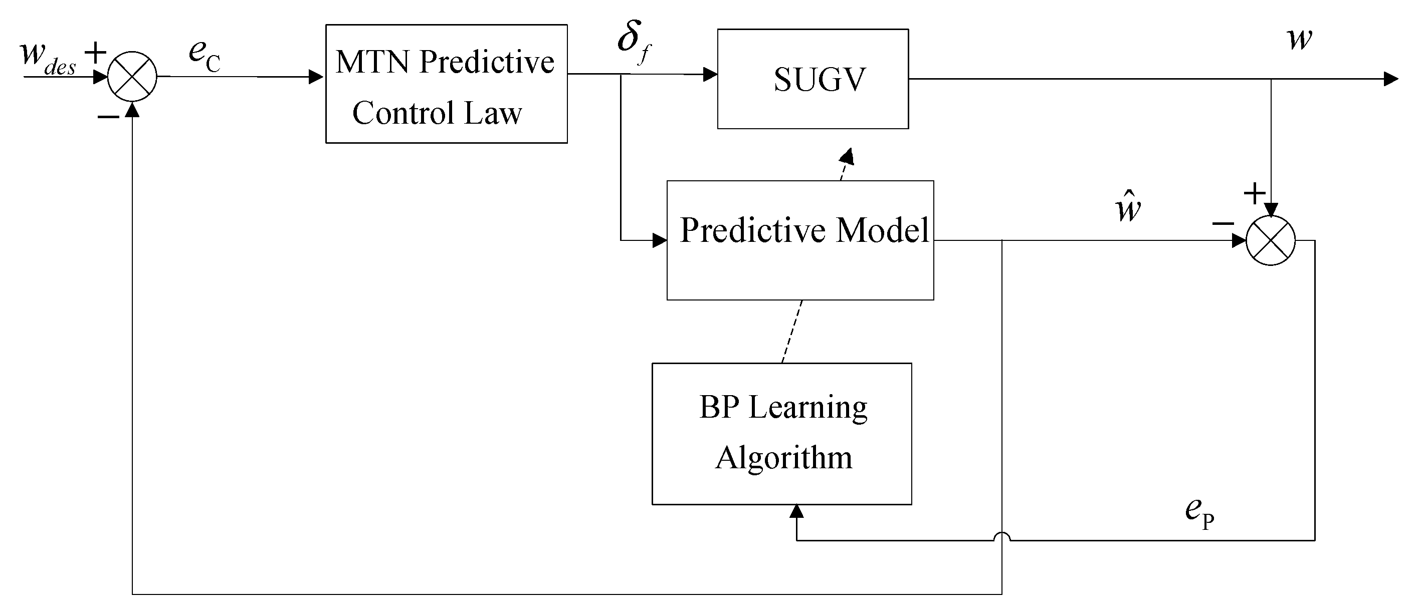
4.4. Scheme of Predictive Control with the Differential Term Based on the MTN Model

An improved predictive control scheme on the basis of the MTN is proposed for tracking control of SUGVs. First, a predictive model is constructed as follows: (1) the MTN is used as a predictive model to construct a SUGV model; and (2) the BP algorithm is used as its learning algorithm. Second, a predictive control law is designed to control the SUGV. The frame diagram of the improved MTN predictive control system is shown in Figure 3. The front wheel steering angle ${\delta }_f$ is used as the control input, which is equivalent to the $u(k)$ mentioned above. The yaw velocity $w$ is used as the system output, which is equivalent to the $y(k)$ mentioned above. The predictive model output $\widehat{w}$ is equivalent to the $\widehat{y}(k)$ mentioned above. The desired yaw velocity $w_{des}$ is used as the system input, which is equivalent to the $r(k)$ mentioned above.

The specific steps are as shown in Algorithm 1.

Algorithm 1 Scheme of MTN Predictive Control with the Differential Term

Step 1: Construct MTN predictive model; (1) Initialize system input and output; (2) Ascertain structure of MTN predictive model; (3) Update ${\mathit{w}}_{\mathrm{P}}(k)$ with Equation (12); Step 2: Construct MTN predictive control law; (1) Construct the quadratic performance index, shown as (13); (2) Update $u(k)$ with Equation (14); Step 3: Construct an improved predictive control law to control SUGV based on MTN predictive control law; (1) Construct the quadratic performance index with differential term, shown as (15); (2) Update the $u(k)$ with Equation (17); Step 4. Implement the tracking control for the SUGV.

5. Simulation Results and Discussion

5.1. Simulation Results

SUGVs have a wide range of applications, such as delivery, sanitation, and mining. A tracking control experiment on a SUGV is described here [44,45]. Moreover, the traditional MTN predictive control scheme [24] and the recurrent radial basis (RBF) model predictive control scheme [46] are used for comparison. According to the vehicle dynamics model, as shown in (7), the tracking effect is demonstrated by accurately tracking the desired yaw velocity signal. The control input and output variables are the front wheel steering angle ${\delta }_f$ and the yaw velocity $w$, respectively. The mathematical relationship between the desired path curve $y=f(x)$ and the desired yaw velocity signal is as follows [44,45]:

$$w_{des}=v_{des}{k}_{des}$$

(23)

$$k_{des}=\frac{d^{2}y/d{x}^2}{{(1+(dy/dx{)}^2)}^{3/2}}$$

(24)

where $w_{des}$ is the desired yaw velocity, $v_{des}$ is the desired speed, and $k_{des}$ represents the curvature of the desired road.

Specific parameters of the SUGV were set as follows: $M=0.1 \mathrm{kg}$, $l_f=0.1 \mathrm{m}$, $l_r=0.1 \mathrm{m}$, $I_z=0.4 \mathrm{kg}/{\mathrm{m}}^2$, $v_x=1 \mathrm{m}/\mathrm{s}$, $L=0.6 \mathrm{m}$, $C_f=0.6 \mathrm{N}/\mathrm{rad}$, and $C_r=0.6 \mathrm{N}/\mathrm{rad}$.

Two cases were considered: without noise and with noise. The same parameters were adopted for each of them to verify the performance of the proposed scheme.

Remark 1.

In the following, D-MTNC is our proposed scheme; MTNC is the traditional MTN predictive control scheme; and RBFC is the RBF model predictive control scheme.

Remark 2.

In the following figures, wdes represents the given reference signal; yMTNC is the traditional MTN predictive control scheme; yD-MTNC is the proposed predictive control scheme; yRBFC is the RBF model predictive control scheme; and eMTNC, eD-MTNC, and eRBFC represent the corresponding tracking errors.

We consider the control effect of the yaw velocity tracking step signal. The given reference signal is $w_{des}=1$. The parameters of D-MTNC, MTNC, and RBFC were set as follows.

The MTN predictive model adopts a 4-15-1 structure with four inputs and two powers. The initial value of the weight coefficient vector for the BP algorithm is ${\widehat{\mathit{w}}}_{\mathrm{P}}(0)=0$ and the learning factor is $\mu =0.5$.

For the D-MTNC control law parameters, the control effort weighting factor was set to $1/\epsilon =0.1$ and the differential term weighting factor was set to $\gamma =0.005$.

For the MTNC control law parameters, the control effort weighting factor was set to $1/\epsilon =0.1$.

The RBF predictive model adopts a 4-18-1 structure. The initial value of the weight coefficient vector for the BP algorithm is ${\widehat{\mathit{w}}}_{\mathrm{P}}(0)=0$ and the learning factor is $\mu =0.9$.

For the RBFC control law parameters, the control effort weighting factor was set to $1/\epsilon =0.9$.

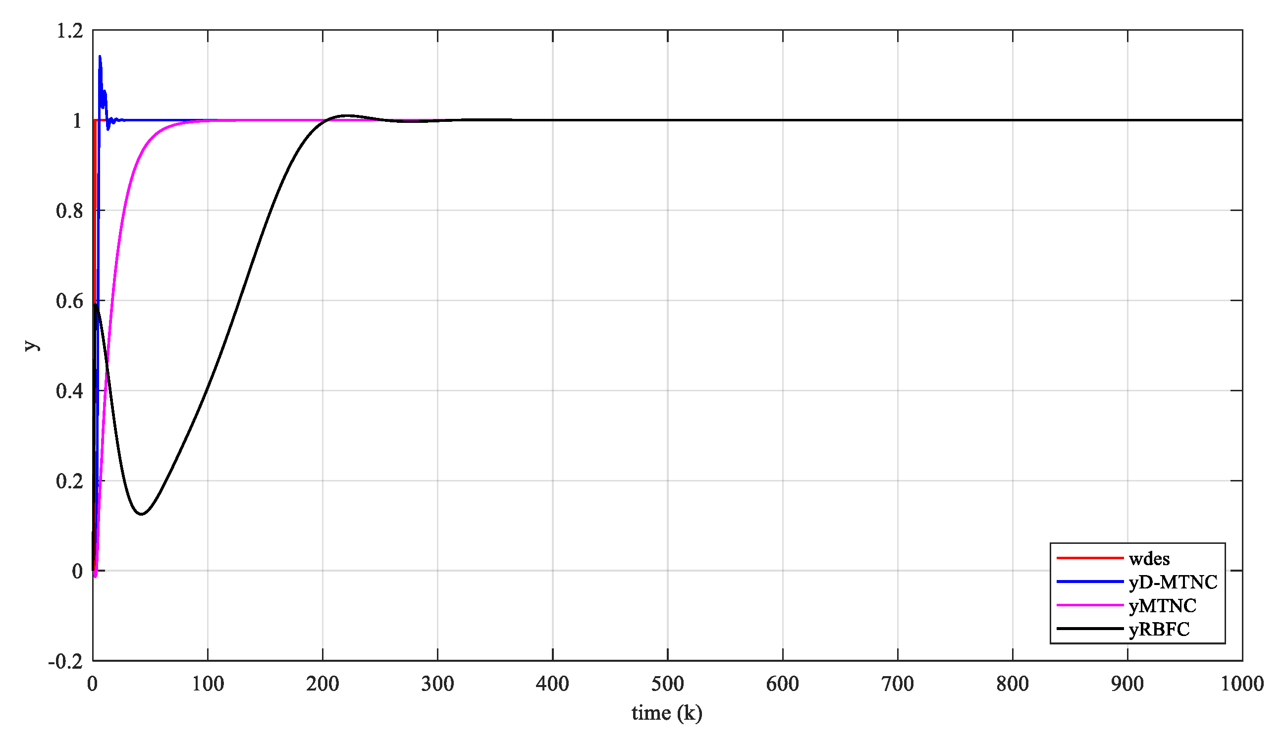
5.1.1. Without Noise

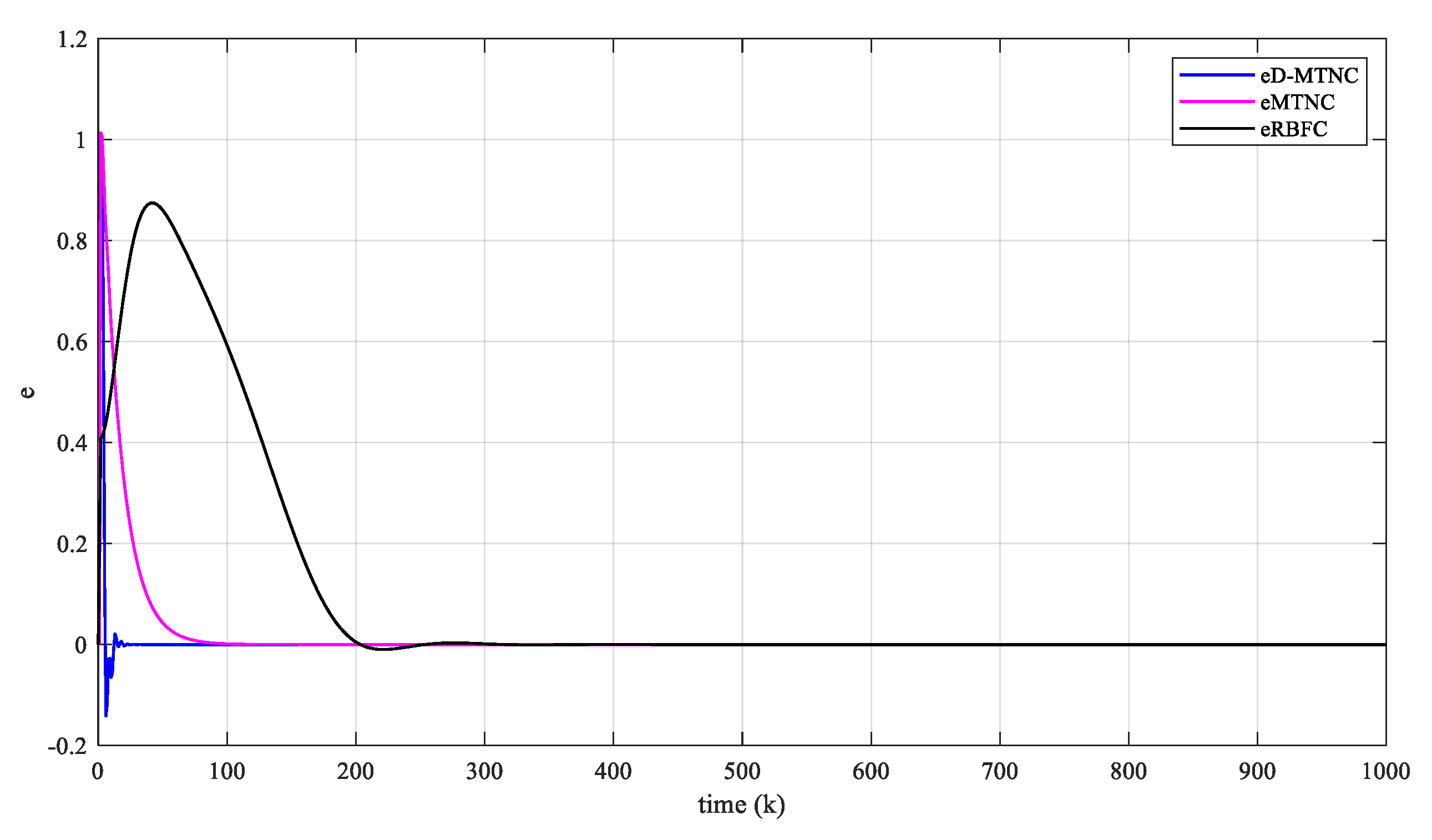
Figure 4 shows the tracking trajectory and Figure 5 shows the tracking error. Figure 4 and Figure 5 show that the SUGV reaches the desired speed quickly and accurately. Our proposed scheme tracks the given reference signal at $k=5$, whereas the traditional MTN predictive control scheme and the RBF predictive control scheme track the reference signal at $k=70$ and $k=250$, respectively. These results verify that the improved predictive control scheme has a better control effect and faster convergence than the other schemes.

5.1.2. With Noise

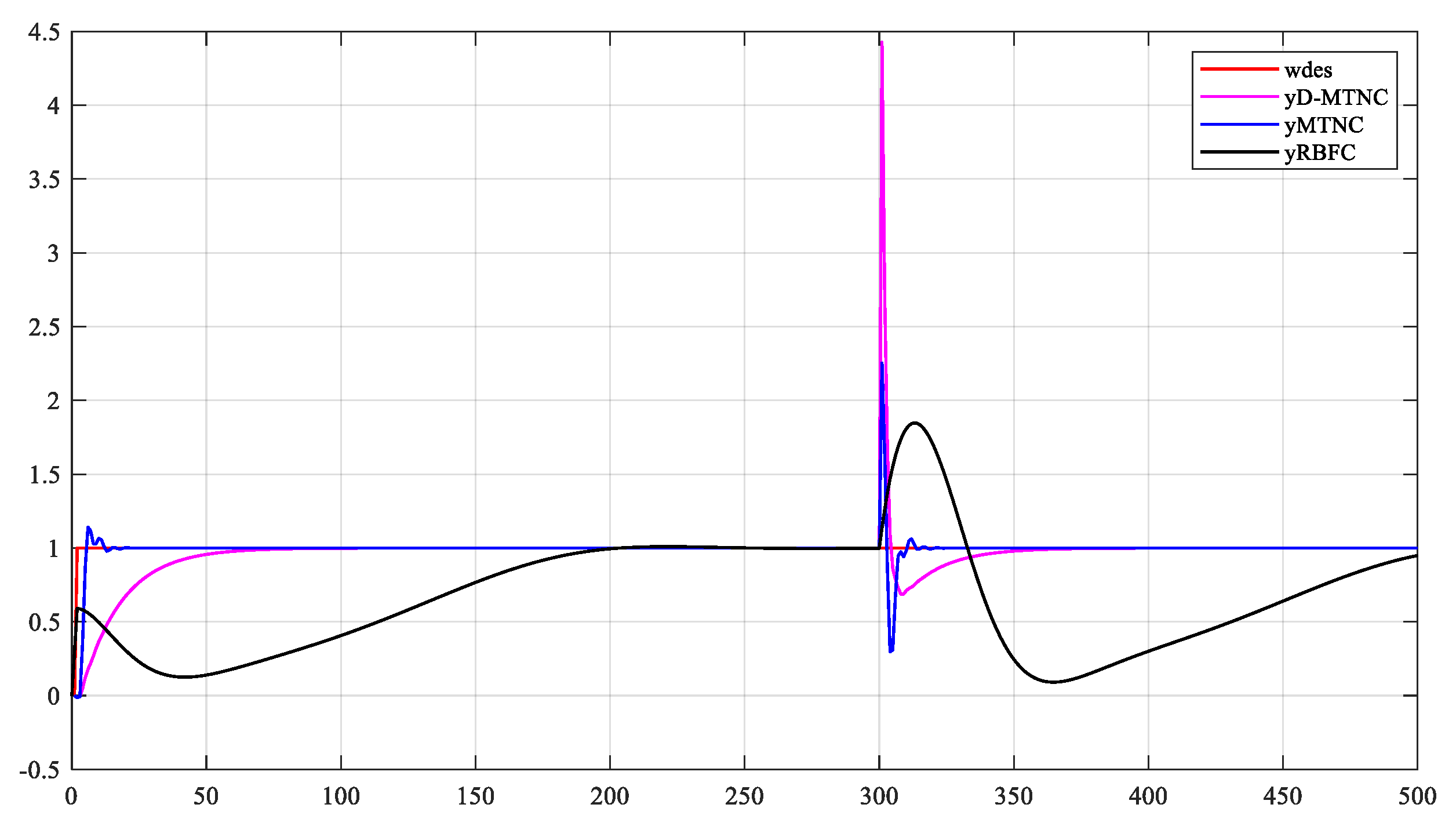
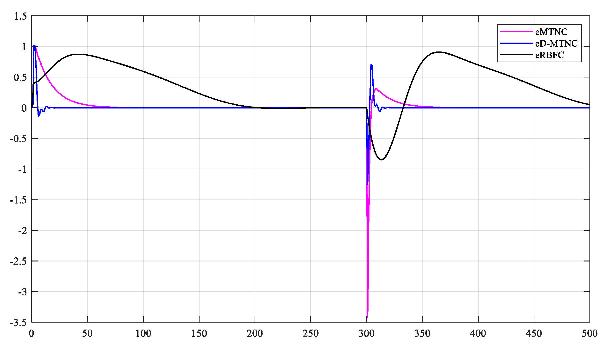
To verify the robustness of the proposed control scheme, Gaussian white noise and 100 times the noise were added to the system. Regarding the Gaussian white noise, it exhibits a mean of 0 and a standard deviation of 0.2 at the 300th time point.

Figure 6 shows the tracking trajectory and Figure 7 shows the tracking error. From Figure 6 and Figure 7, when 100 times the Gaussian white noise is added at the 300th time point to the system, there is a sharp change at the 300th time point, but the proposed control scheme has a quick response, which retracks the reference more quickly than the other schemes. These results verify that the improved predictive control scheme has a good control effect and good robustness.

5.2. Discussion

For tracking control of SUGVs, the above results show that the proposed method has good performance and tracks the reference signal quickly and accurately. To verify the robustness of the proposed scheme, sharp noise was added. The results of the experiment in terms of tracking, robustness, and real-time performance all show that the proposed scheme has better performance than MTNC and RBFC.

Regarding the choice of model structure, what needs illustration is that the MTN predictive model adopted a 4-15-1 structure and the RBF predictive model adopted a 4-18-1 structure in this paper. The MTN structure depends on the middle layer’s nodes when the input and output layer are confirmed. The middle layer’s nodes rely on the input layer’s nodes and the power item. The MTN predictive model’s structure is shown in Figure 1. From Figure 1, when the input layer had four nodes and the number of power items was 2, the number of product items was 15. The RBF hidden layer’s nodes depend on the history of multiple experiments, and we chose 18 nodes for the hidden layer here.

The proposed scheme showed good performance in tracking control of the SUGV. However, SUGVs have a wide range of applications, such as delivery, sanitation, and mining. When facing these practical scenarios, the proposed method needs to be experimentally validated and the appropriate parameters need to be selected according to the actual situation.

6. Conclusions

An improved predictive control scheme based on the MTN was proposed for tracking control of SUGVs. The traditional objective function was improved to obtain a predictive objective function with the differential term. The optimal control quantity was given in real time through iterative optimization. A tracking control experiment on a SUGV was carried out to verify the effectiveness of the proposed scheme. The results show that the proposed scheme is effective and has good real-time, robustness, and convergence performance, which ensure that the vehicle can quickly and accurately track the desired yaw velocity signal, and is superior to the traditional MTN and RBF predictive control schemes.

The proposed improved MTN predictive control scheme developed in the present paper shows great promise but requires further study. For example, the proposed scheme could be applied to different complex driving scenarios, and some complicated conditions could be considered, such as an actuator failure or input constraints.

References

- Wang, H.B.; Zuo, J.S.; Liu, S.D.; Zheng, W.; Wang, L. Model-free adaptive control of steady-state drift of unmanned vehicles. Control Theory Appl. 2021, 38, 23–32. (In Chinese) [Google Scholar]
- Elbanhawi, M.; Simic, M.; Jazar, R. In the passenger seat: Investigating ride comfort measures in autonomous cars. IEEE Intel. Transp. Syst. Mag. 2015, 7, 4–17. [Google Scholar] [CrossRef]
- Kim, S.; Gwon, G.P.; Hur, W.S.; Hyeon, D.; Kim, D.-Y.; Kim, S.-H.; Kim, D.-K.; Lee, S.-H.; Lee, S.; Shin, M.-O.; et al. Autonomous campus mobility services using driverless taxi. IEEE Trans. Intel. Transp. Syst. 2017, 18, 3513–3526. [Google Scholar] [CrossRef]
- Kramberger, T.; Potocnik, B. LSUN-stanford car dataset: Enhancing large-scale car image datasets using deep learning for usage in GAN training. Appl. Sci. 2020, 10, 4913. [Google Scholar] [CrossRef]
- Shen, K.; Wang, M.; Fu, M.; Yang, Y.; Yin, Z. Observability analysis and adaptive information fusion for integrated navigation of unmanned ground vehicles. IEEE Trans. Ind. Electron. 2020, 67, 7659–7668. [Google Scholar] [CrossRef]
- Wang, H.; Yuan, S.; Guo, M.; Chan, C.-Y.; Li, X.; Lan, W. Tactical driving decisions of unmanned ground vehicles in complex highway environments: A deep reinforcement learning approach. Proc. Inst. Mech. Eng. Part D J. Automob. Eng. 2021, 235, 1113–1127. [Google Scholar] [CrossRef]
- Zhang, H.; Zhang, H.M.; Wang, Z.P. Event-triggered predictive path following control for unmanned autonomous vehicle. Control Decis. 2019, 34, 2421–2427. (In Chinese) [Google Scholar]
- Kaur, K.; Rampersad, G. Trust in driverless cars: Investigating key factors influencing the adoption of driverless cars. J. Eng. Technol. Manag. 2018, 48, 87–96. [Google Scholar] [CrossRef]
- Chen, G.; Zhang, W.G.; Zhang, X.N. Speed tracking control of a vehicle robot driver system using multiple sliding surface control schemes. Int. J. Adv. Robot Syst. 2013, 10, 1–9. [Google Scholar] [CrossRef] [Green Version]
- Song, C.; Zhao, R.; Yang, H.; Zeng, Z.; Wu, J. Using fuzzy control for parallel-inverter system with nonlinear-load. In Proceedings of the 2010 International Conference on Electrical Machines and Systems, Incheon, Korea, 10–13 October 2010; pp. 193–197. [Google Scholar]
- Niu, H.; Bhowmick, C.; Jagannathan, S. Attack detection and approximation in nonlinear networked control systems using neural networks. IEEE Trans. Neural Netw. Learn. Syst. 2020, 31, 235–245. [Google Scholar] [CrossRef]
- Zhao, J.; Sun, J.; Cai, Z.; Wang, L.; Wang, Y. End-to-End deep reinforcement learning for image-based UAV autonomous control. Appl. Sci. 2021, 11, 8419. [Google Scholar] [CrossRef]
- Mehmood, A.; Zameer, A.; Ling, S.H.; Rehman, A.U.; Raja, M.A.Z. Integrated computational intelligent paradigm for nonlinear electric circuit models using neural networks, genetic algorithms and sequential quadratic programming. Neural Comput. Appl. 2020, 32, 10337–10357. [Google Scholar] [CrossRef]
- Wu, Z.; Rincon, D.; Christofides, P.D. Process structure-based recurrent neural network modeling for model predictive control of nonlinear processes. J. Process Control 2020, 89, 74–84. [Google Scholar] [CrossRef]
- Piche, S.; Sayyar-Rodsari, B.; Johnson, D.; Gerules, M. Nonlinear model predictive control using neural networks. IEEE Control Syst. Mag. 2000, 20, 53–62. [Google Scholar]
- Rummelhart, D.E.; Hinton, G.E.; Williams, R.J. Learning representations by back propagating errors. Nature 1986, 323, 533–536. [Google Scholar] [CrossRef]
- Zhou, B.; Yan, H.S. Financial time series forecasting based on wavelet and multi-dimensional Taylor network dynamics model. Syst. Eng.-Theory Pract. 2013, 33, 2654–2662. (In Chinese) [Google Scholar]
- Yan, H.S.; Kang, A.M. Asymptotic tracking and dynamic regulation of SISO nonlinear system based on discrete multi-dimensional Taylor network. IET Control Theory Appl. 2017, 11, 1619–1626. [Google Scholar] [CrossRef]
- Lin, Y.; Yan, H.S.; Zhou, B. Nonlinear time series prediction method based on multi-dimensional Taylor network and its applications. Control Decis. 2014, 29, 795–801. (In Chinese) [Google Scholar]
- Li, C.L.; Yan, H.S. Nonlinear time-delay system identification and prediction based on multi-dimensional Taylor network and IPSO. J. Grey Syst. 2018, 30, 96–109. [Google Scholar]
- Li, C.L.; Yan, H.S.; Zhang, J.J. Multi-dimensional Taylor network adaptive predictive control for singleinput single-output nonlinear systems with input time-delay. Trans. Inst. Meas. Control 2022, 44, 595–608. [Google Scholar] [CrossRef]
- Zhang, J.J.; Yan, H.S. MTN optimal control of MIMO non-affine nonlinear time-varying discrete systems for tracking only by output feedback. J. Frankl. Inst. 2019, 356, 4304–4334. [Google Scholar] [CrossRef]
- Zhang, C.; Yan, H.S. Identification and adaptive Multi-dimensional Taylor network control of single-input single-output non-linear uncertain time-varying systems with noise disturbances. IET Control Theory Appl. 2019, 13, 841–853. [Google Scholar] [CrossRef]
- Li, C.L.; Ma, X.S.; Zhang, J.J. Nonlinear system predictive control using a multi-dimensional Taylor network. Trans. Inst. Meas. Control 2019, 41, 3396–3405. [Google Scholar] [CrossRef]
- Schwarting, W.; Alonso-Mora, J.; Paull, L.; Karaman, S.; Rus, D. Safe nonlinear trajectory generation for parallel autonomy with a dynamic vehicle model. IEEE Trans. Intel. Transp. 2018, 19, 2994–3008. [Google Scholar] [CrossRef] [Green Version]
- Li, R.; Zhang, L.; Han, L.; Wang, J. Multiple vehicle formation control based on robust adaptive control algorithm. IEEE Intel. Transp. Syst. 2017, 9, 41–51. [Google Scholar] [CrossRef]
- Zhen, Z.; Tao, G.; Yu, C.; Xue, Y. A multivariable adaptive control scheme for automatic carrier landing of UAV. Aerosp. Sci. Technol. 2019, 92, 714–721. [Google Scholar] [CrossRef]
- Tagne, G.; Talj, R.; Charara, A. Higher-order sliding mode control for lateral dynamics of autonomous vehicles, with experimental validation. In Proceedings of the 2013 IEEE Intelligent Vehicles Symposium (IV), Gold Coast, QLD, Australia, 23–26 June 2013; pp. 678–683. [Google Scholar]
- Wang, P.; Gao, S.; Li, L.; Cheng, S.; Zhao, L. Automatic steering control strategy for unmanned vehicles based on robust backstepping sliding mode control theory. IEEE Access 2019, 7, 64984–64992. [Google Scholar] [CrossRef]
- Yu, L.; Yan, X.; Kuang, Z.; Chen, B.; Zhao, Y. Driverless bus path tracking based on fuzzy pure pursuit control with a front axle reference. Appl. Sci. 2020, 10, 230. [Google Scholar] [CrossRef] [Green Version]
- Chen, Y.; Hu, C.; Qin, Y.; Li, M.; Song, X. Path planning and robust fuzzy output-feedback control for unmanned ground vehicles with obstacle avoidance. Proc. Inst. Mech. Eng. Part D J. Automob. Eng. 2021, 235, 933–944. [Google Scholar] [CrossRef]
- Ji, X.W.; He, X.K.; Chen, L.; Liu, Y.; Wu, J. Adaptive-neural-network-based robust lateral motion control for autonomous vehicle at driving limits. Control Eng. Pract. 2018, 76, 41–53. [Google Scholar] [CrossRef]
- Kabzan, J.; Hewing, L.; Liniger, A.; Zeilinger, M.N. Learning-based model predictive control for autonomous racing. IEEE Robot Autom. Lett. 2019, 4, 3363–3370. [Google Scholar] [CrossRef] [Green Version]
- Zhao, K.; Wang, C.; Xaio, G.; Li, H.; Ye, J.; Liu, Y. Research for nonlinear model predictive controls to laterally control unmanned vehicle trajectory tracking. Appl. Sci. 2020, 10, 6034. [Google Scholar] [CrossRef]
- Kayacan, E.; Ramon, H.; Saeys, W. Robust trajectory tracking error model-based predictive control for unmanned ground vehicles. IEEE-ASME Trans. Mech. 2016, 21, 1–9. [Google Scholar] [CrossRef]
- Bozek, P.; Karavaev, Y.L.; Ardentov, A.A. Neural network control of a wheeled mobile robot based on optimal trajectories. Int. J. Adv. Robot Syst. 2020, 17, 1–10. [Google Scholar] [CrossRef] [Green Version]
- Cummings, M.L.; How, J.P.; Whitten, A.; Toupet, O. The impact of human-automation collaboration in decentralized multiple unmanned vehicle control. Proc. IEEE 2012, 100, 660–671. [Google Scholar] [CrossRef]
- Donmez, B.; Nehme, C.; Cummings, M.L. Modeling workload impact in multiple unmanned vehicle supervisory control. IEEE Trans. Syst. Man Cybern.-Part A Syst. Hum. 2010, 40, 1180–1190. [Google Scholar] [CrossRef]
- Klambauer, G. Mathematical Analysis; Marcel Dekker Inc.: New York, NY, USA, 1975. [Google Scholar]
- Cowan, C.F.N.; Grant, P.M. (Eds.) Adaptive Filters; Prentice-Hall, Inc.: Englewood Cliffs, NJ, USA, 1985. [Google Scholar]
- Al-Batah, M.S.; Isa, N.A.M.; Zamli, K.Z.; Azizli, K.A. Modified recursive least squares algorithm to train the hybrid multilayered perceptron (HMLP) network. Appl. Soft Comput. 2010, 10, 236–244. [Google Scholar] [CrossRef]
- Ku, C.C.; Lee, K.Y. Diagonal recurrent neural networks for dynamic systems control. IEEE Trans. Neural Netw. 1995, 6, 144–156. [Google Scholar]
- Peng, J.Z.; Dubay, R. Identification and adaptive neural network control of a DC motor system with dead-zone characteristics. ISA Trans. 2011, 50, 588–598. [Google Scholar] [CrossRef] [PubMed]
- Nguyen, T.W.; Catoire, L.; Garone, E. Control of a quadrotor and a ground vehicle manipulating an object. Automatica 2019, 105, 384–390. [Google Scholar] [CrossRef]
- Ren, H.; Karimi, H.R.; Lu, R.; Wu, Y. Synchronization of network systems via aperiodic sampled-data control with constant delay and application to unmanned ground vehicles. IEEE Trans. Ind. Electron. 2020, 67, 4980–4990. [Google Scholar] [CrossRef]
- Tavoosi, J.; Mohammadzadeh, A. A new recurrent radial basis function network-based model predictive control for a power plant Boiler. Int. J. Eng. 2021, 34, 667–675. [Google Scholar]
Figure 1.
The SUGV model.
Figure 2.
Diagram of the MTN.
Figure 3.
Block diagram of the improved MTN predictive control system.
Figure 4.
The tracking trajectory without noise.
Figure 5.
The tracking error without noise.
Figure 6.
The tracking trajectory with noise.
Figure 7.
The tracking error with noise.
Publisher’s Note: MDPI stays neutral with regard to jurisdictional claims in published maps and institutional affiliations. |
© 2022 by the authors. Licensee MDPI, Basel, Switzerland. This article is an open access article distributed under the terms and conditions of the Creative Commons Attribution (CC BY) license (https://creativecommons.org/licenses/by/4.0/).
Share and Cite
MDPI and ACS Style
Wu, Y.; Li, C.; Yuan, C.; Li, M.; Li, H. Predictive Control for Small Unmanned Ground Vehicles via a Multi-Dimensional Taylor Network. Appl. Sci. 2022, 12, 682. https://0-doi-org.brum.beds.ac.uk/10.3390/app12020682
AMA Style
Wu Y, Li C, Yuan C, Li M, Li H. Predictive Control for Small Unmanned Ground Vehicles via a Multi-Dimensional Taylor Network. Applied Sciences. 2022; 12(2):682. https://0-doi-org.brum.beds.ac.uk/10.3390/app12020682
Chicago/Turabian StyleWu, Yuzhan, Chenlong Li, Changshun Yuan, Meng Li, and Hao Li. 2022. "Predictive Control for Small Unmanned Ground Vehicles via a Multi-Dimensional Taylor Network" Applied Sciences 12, no. 2: 682. https://0-doi-org.brum.beds.ac.uk/10.3390/app12020682
Note that from the first issue of 2016, this journal uses article numbers instead of page numbers. See further details here.