Rigid-Flexible Coupled Dynamic and Control for Thermally Induced Vibration and Attitude Motion of a Spacecraft with Hoop-Truss Antenna

Abstract

As space exploration activities are developing rapidly, spacecraft with large antennas have gained wide acceptance in providing reliable telecommunications and astrophysical observations. In this paper, the dynamic responses and control strategy for a spacecraft with a large hoop-truss antenna under solar flux shock are studied. According to the momentum and angular momentum principle, the rigid-flexible coupled rotational dynamic equation and the translational dynamic equation of the system are established, which include the attitude motion of the rigid main body and the vibration of the antenna. Then, a finite element model of the antenna is established to analytically obtain the corresponding vibration modal shape matrix and natural frequencies. Last, the coupled responses for the attitude motion and vibration are investigated. The corresponding control strategy is designed based on a double-loop structure sliding mode control method. The Lyapunov method is used to demonstrate the global asymptotic stability of the system. Simulations verify the effectiveness of the proposed rigid-flexible coupled model and control strategy.

1. Introduction

Modern spacecraft are usually equipped with large flexible appendages, such as deployable antennas, robot arms, and solar panels, which may cause the spacecraft to have extremely high flexibility and low-frequency vibration modes [1]. The solar flux shock is one of the most important excitations that induce those low-frequency vibration modes which usually occur during the diurnal or diurnal shifts in orbit. The sudden changes in the thermal load can cause temperature gradients in the appendage and further lead to thermal stress, deformation, and vibrations [2,3]. In addition, vibration can also interact with the attitude motion and attitude maneuver of spacecraft [4], significantly reducing the accuracy of the spacecraft attitude, and even leading to complete failure of the mission [2]. For example, the pointing disruptions were caused by thermal gradients of the Hubble Space Telescope’s solar array [2], and the solar arrays caused the attitude disturbances on the Upper Atmosphere Research Satellite [4]. Thus, the research on the dynamical behaviors and effective control strategies for the coupled attitude and vibration motion is essential and indispensable for spacecraft equipped with large flexible appendages [5,6].

There are many investigations about the modeling methods for rigid spacecraft with flexible appendages. The Hamilton principle was generally used to establish the governing equations for rigid-flexible coupled continuum systems [7,8]. Most investigations focused on appendages with regular shapes such as a beam, plate, or shell. Azimi and Joubaneh [9] derived the coupled control partial differential equation of motion by using the Hamilton principle for the spacecraft with flexible sandwich panels. Cao et al. [10] investigated the coupled model of a spacecraft composed of a rigid platform and two flexible solar arrays. The nonlinear dynamic equations, which remain the second-order coupling terms of axial displacement caused by the transverse motion of solar arrays, were obtained by using the Hamilton principle. The dynamic model of a flexible hub-beam-tip mass system is established and researched by Guo et al. [11]. Axisa and Trompette [12] presented a problem concerning the free vibrations of a set of n axially loaded stretched Bernoulli–Euler beams connected by elastic layers. A normal-mode solution is applied to the governing partial differential equations to derive a set of coupled ordinary differential equations which are used to determine the natural frequencies and mode shapes. Another type of method to model the rigid-flexible system is based on multi-body dynamics. The absolute node coordinate formula (ANCF) and Kane’s method can accurately describe rigid-flexible systems, especially those with large deformation. Hu et al. [13] used Kane’s method to derive the coupled dynamics equation for a rigid body with multiple flexible bodies. Liu et al. [14] used ANCF to derive the dynamics of a single composite laminated plate. García-Vallejo [15] utilized natural coordinates and the ANCF for rigid-flexible multibody systems with flexible beam elements. For flexible appendages with irregular shapes, such as the hoop-truss antennas and inflatable structures, one of the major problems that researchers are faced with is solving the dynamic equation of motion in linear and nonlinear behaviors [16]; the finite element model has advantages in obtaining the frequency and modes analytically [17]. Bergan and Nygard [18] developed the so-called free formulation (FF) for the construction of displacement-based incompatible finite elements. Felippa [19] lifted strict invertibility conditions linking by recasting the free formulation within the framework of a mixed-hybrid functional that allows internal stresses. An efficient thermal–structural coupling finite element method (FEM) formulation for the dynamics of the beam–cable tensegrity structure was developed and validated by Shen [20]. Felippa [21] presented a set of Mathematica modules that organizes numerical integration rules considered useful for finite element work. Xue et al. [3] developed a finite element scheme to solve the thermally induced bending–torsion coupling vibration of thin-walled beams and the thermal and structure coupling was taken into account.

The aforementioned modeling methods provide the basis for solving the thermally induced coupled attitude and vibration problem. Generally, the thermally induced motion of satellite appendages consist of quasi-static deformation and superimposed vibration [4]. Shen and Hu [22] analyzed the flutter problem caused by the thermal impact of the solar panel when the satellite comes in and out of the shadowed area of the Earth. Guo [23] conducted a thermal analysis of the hoop-truss antenna subjected to extreme heat load using the finite element method. Shen [20,24] analyzed flutter stable boundary for the thermoelastic-structure of spatial thin-walled beams under solar radiation.

Through previous studies, it is found that thermal vibration has an important effect on the stability of the system, and this effect is exacerbated by the coupling motion of attitude and vibration. At this time, a control strategy is needed to ensure its stable operation [25]. Among all the control theories, the sliding mode control theory has received a good deal of attention because of its robustness and simplicity. In addition, the sliding mode control theory is suitable for such rigid-flexible systems with profound nonlinearity and modeling uncertainty. Successful applications to practical systems are numerous [25]. Hu [26] designed the discontinuous attitude control law based on sliding mode control theory for adapting the unknown upper bounds of the lumped disturbance so that the limitation of knowing the bound of the disturbance in advance is released. Shahravi [27] used adaptive sliding mode control with a mixed sliding surface to minimize the impact of uncertainty and interference. In order to stabilize the attitude of the flexible spacecraft, Dong et al. [28] proposed a new adaptive fuzzy sliding mode control method to solve the time-delay dynamic model. Qu and Gao [29] used the sliding mode method to control the uniaxial attitude of the flexible spacecraft. Combining the positive position feedback controller and the piezoelectric actuator/sensor on the solar panel area, Hu [30] used an adaptive sliding mode controller to adjust the attitude to suppress vibration.

In conclusion, the coupled rigid-flexible model of spacecraft with irregular appendage can be established effectively based on the finite element model, and the thermally induced coupled dynamical behaviors and control strategy of the satellite’s attitude motion and hoop-truss antenna’s vibration under solar flux shock can be further studied, which is rarely mentioned in references.

The paper is structured as follows. The rigid-flexible coupled dynamic model of spacecraft is derived by using the law of conservation of momentum and angular momentum in Section 2. In Section 3, an effective thermal–structural finite element model is developed to obtain the corresponding natural frequencies and modal shapes analytically. The results are validated by the comparisons with Multiphysics FEA. Finally, the dynamic behaviors of the satellite’s attitude motion and hoop-truss antenna’s vibration are investigated. Meanwhile, the attitude controller is designed using variable structure sliding mode control theory in Section 4. The conclusions are drawn in Section 5.

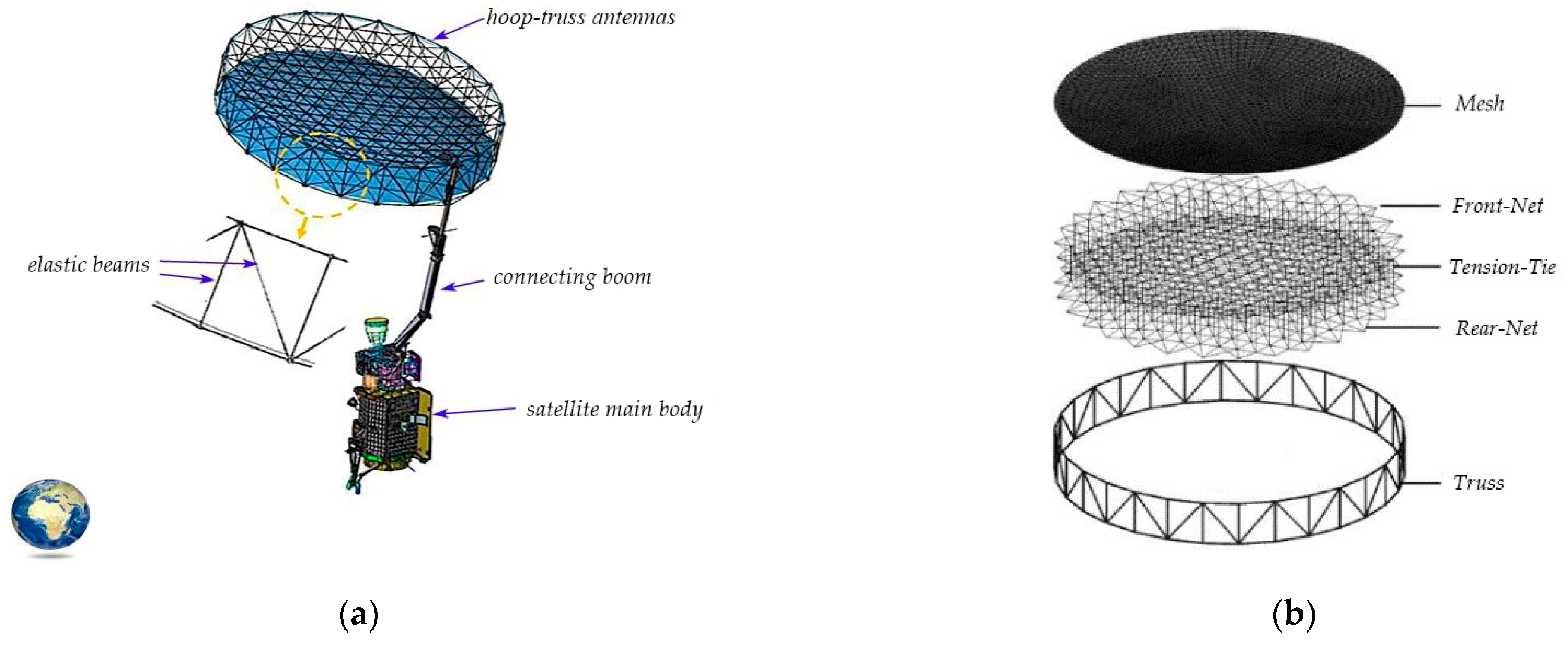
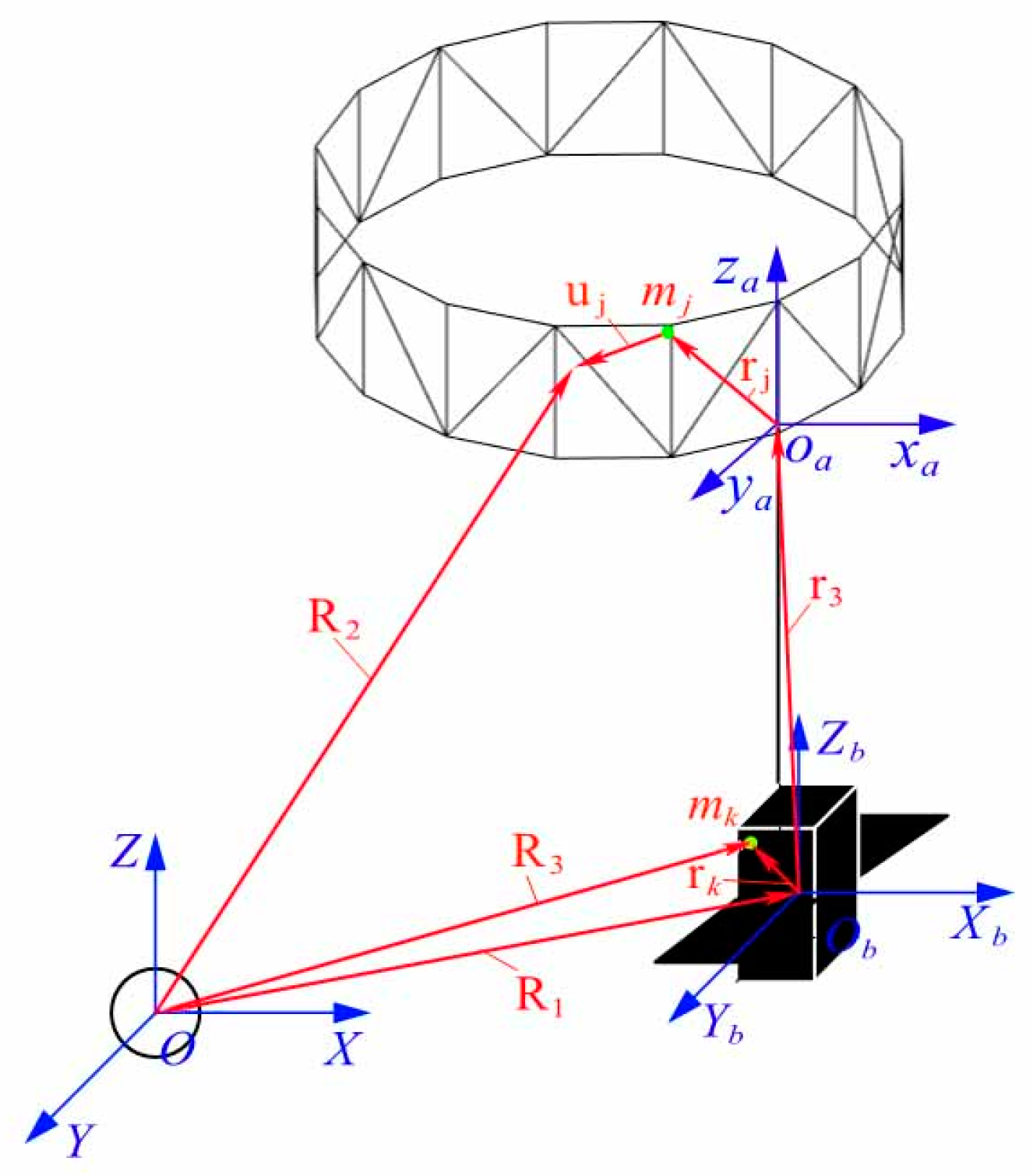
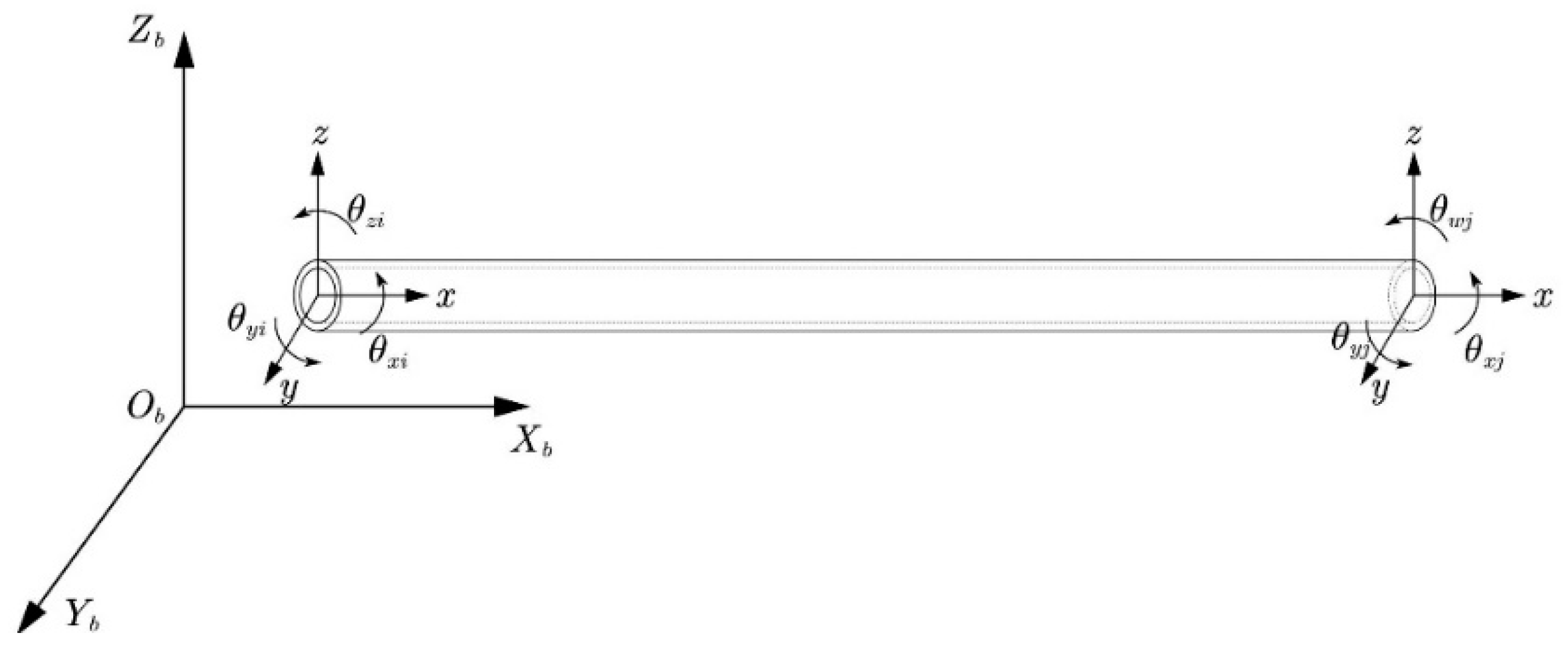
2. Rigid-Flexible Model for Spacecraft with Hoop-Truss Antenna

In this section, a spacecraft similar to NASA’s Soil Moisture Active Passive (SMAP) is considered, which is composed of a rigid main body, a flexible antenna, and rigid connecting booms, as shown in Figure 1a. The antenna generally consists of the mesh, front-net, tension-tie, rear-net, and truss, as shown in Figure 1b. In addition, the hoop-truss antenna consists of several elastic beams and the connecting boom serves only as a connection whose mass and shape are ignored. The gravitational effect is also neglected for simplicity. Only the truss is considered for the following modeling and analysis.

To describe the rigid-body motion of the spacecraft and the elastic displacement of the flexible hoop-truss, three coordinate systems are defined and shown in Figure 2. The O-XYZ is the inertial coordinate system with its origin located at the center of the Earth. The e = [e_x e_y e_z]^T denotes the unit vectors. The O_b-x_by_bz_b is defined as a body-fixed coordinate system and denoted by b = [b_x b_y b_z]^T which rotates around O-XYZ with angular velocity ω. O_b is the center of mass of the rigid body, and three axes are all parallel to the principal axes of inertia. The antenna coordinate system O_a-x_ay_az_a denoted by a = [a_x a_y a_z]^T is located at the point O_a which is the junction point of the rigid body and the antenna. Three axes are parallel to the axes of the O_b-x_by_bz_b coordinate system. The antenna’s angular velocity with respect to O_b-x_by_bz_b is ω_a. In Figure 2, R₁, R₂, and R₃ represent the vector from the Earth’s center to the mass center of the rigid body O_b, mass element m_k of the rigid body, and mass element m_j of the antenna, respectively. r₃ represents the vector from O_b to O_a, r_j represents the vector from O_a to m_j, r_j represents the vector from O_b to m_k, and u_j is the displacement of the mass element m_j. It can be found that R₂ = R₁ + r₃ + r_j + u_j and R₃ = R₁ + r_k.

Based on the momentum and angular momentum principle, the rotational dynamic equation and the translational dynamic equation can be written as:

$${\displaystyle \sum _A{m}_j\left(r_3+r_j+u_j\right)\times {\ddot{R}}_2}+{\displaystyle \sum _B{r}_k\times m_k}{\ddot{R}}_3=W$$

(1)

$${\displaystyle \sum _A{m}_j{\ddot{R}}_2}+{\displaystyle \sum _B{m}_k{\ddot{R}}_3}=F$$

(2)

where W denotes the total external moments and F denotes the total external forces. A, B denote the sum with respect to the antenna and the satellite body, respectively.

The velocity vector of the mass element m_j on the antenna can be expressed in O-XYZ as:

$${\dot{R}}_2={\dot{R}}_1+{\left({\dot{r}}_3+{\dot{r}}_j+{\dot{u}}_j\right)}^b+\omega \times \left(r_3+r_j+u_j\right)$$

(3)

where the superscript ‘b’ denotes derivative with respect to the O_b-x_by_bz_b. Since ${({\dot{r}}_3)}^b=0$ and ${({\dot{r}}_j)}^a=0$, we can obtain the velocity in matrix form as:

$${\dot{R}}_2=e^{\mathrm{T}}{\dot{R}}_1+a^T{\left({\dot{u}}_j\right)}^a-a^T\left(r_j{}^{\mathrm{X}}+u_j{}^{\mathrm{X}}\right){\mathsf{\omega }}_a-b^T\left(r_3{}^{\mathrm{X}}+A_{ab}{}^T\left(r_j{}^{\mathrm{X}}+u_j{}^{\mathrm{X}}\right)A_{ab}\right)\mathsf{\omega }$$

(4)

where the subscript ‘a’ denotes derivative with respect to the O_a-x_ay_az_a. A_ab, A_be, and A_ae denote the transformation matrix from the O_b-x_by_bz_b to O_a-x_ay_az_a, the O-XYZ to the O_b-x_by_bz_b, and the O-XYZ to O_a-x_ay_az_a, respectively. The (X)^X denotes X’s anti-symmetric diagonal matrix. Then, the acceleration of m_j can be obtained as:

$$\begin{array}{ll}{\ddot{R}}_2& =a^T{A}_{ae}{\ddot{R}}_1+a^T{\left({\ddot{u}}_j\right)}^a-a^T\left(r_j{}^{\mathrm{X}}+u_j{}^{\mathrm{X}}\right){\dot{\omega }}_a-a^T\left(A_{ab}{r}_3{}^{\mathrm{X}}{A}_{ba}+r_j{}^{\mathrm{X}}+u^{\mathrm{X}}\right)A_{ab}\dot{\omega }\\ & -a^T{\dot{u}}_j{}^{\mathrm{X}}\left(2A_{ab}\mathsf{\omega }+{\mathsf{\omega }}_a\right)-a^T\left[{\left(2A_{ab}\mathsf{\omega }\right)}^{\mathrm{X}}+{\mathsf{\omega }}_a{}^{\mathrm{X}}\right]\left(r_j{}^{\mathrm{X}}+u_j{}^{\mathrm{X}}\right){\mathsf{\omega }}_a\\ & -a^T{\left(A_{ab}\mathsf{\omega }\right)}^{\mathrm{X}}\left(A_{ab}{r}_3{}^{\mathrm{X}}{A}_{ba}+r_j{}^{\mathrm{X}}+u_j{}^{\mathrm{X}}\right)A_{ab}\mathsf{\omega }\end{array}$$

(5)

Neglecting the higher orders of ω, ω_a, u_j, we obtained,

$$\begin{array}{ll}{\ddot{R}}_2& =a^T{A}_{ae}{\ddot{R}}_1+a^T{\left({\ddot{u}}_j\right)}^a-a^T{r}_j{}^{\mathrm{X}}{\dot{\omega }}_a-a^T\left(A_{ab}{r}_3{}^{\mathrm{X}}{A}_{ba}+r_j{}^{\mathrm{X}}\right)A_{ab}\dot{\omega }\\ & -a^T{\left(A_{ab}\mathsf{\omega }\right)}^{\mathrm{X}}\left(A_{ab}{r}_3{}^{\mathrm{X}}{A}_{ba}+r_j{}^{\mathrm{X}}\right)A_{ab}\mathsf{\omega }\end{array}$$

(6)

Similarly, for the mass element m_k of the rigid body, the velocity and acceleration are expressed as follows:

$${\dot{R}}_3=e^T{\dot{R}}_1-b^T{r}_k^{\mathrm{X}}\mathsf{\omega }$$

(7)

$${\ddot{R}}_3=b^T{A}_{be}{\ddot{R}}_1-b^T{r}_k{}^{\mathrm{X}}\dot{\omega }-b^T{\mathsf{\omega }}^{\mathrm{X}}{r}_k{}^{\mathrm{X}}\mathsf{\omega }$$

(8)

In order to study the coupling dynamics of attitude and vibration, we express the elastic displacement u_j in the form of independent modal coordinates as:

$$u_j={\displaystyle \sum _{i=1}^n{Q}_i{\eta }_i}=Q\eta$$

(9)

where Q = [Q₁,…,Q_n], η = [η₁,…, η_n]^T, η_i is the ith modal coordinate, and Q_i is the modal vector representing the ith modal shape of the structure. Since the structure of the hoop-truss antenna is relatively complex, it is difficult to find the appropriate assumed modal shapes. Both η_i and Q_i will be obtained by analytical finite element method in the next section.

Substituting Equation (6), Equation (8) into Equation (1) yields the rotational equations of motion:

$$S_b{a}_1-I_b\dot{\omega }-I_{\mathsf{\omega }}\omega +H_{ab}{A}_{be}{a}_1+H_{ab}{P}_a{\ddot{\eta }}_a-\left(I_b^{ab}+I^{ab}\right){\dot{\omega }}_a-I_{ab}^b\dot{\omega }-I_{\mathsf{\Omega }ab}^b\omega =W$$

(10)

Substituting Equation (6), Equation (8) into Equation (2) yields an equation of motion for translational motion:

$$\begin{array}{l}{M}_b{A}_{ae}{a}_1-S_b{A}_{ab}\dot{\omega }-{\left(A_{ab}\omega \right)}^{\mathrm{X}}{S}_b{A}_{ab}\omega +M_a{A}_{ae}{a}_1\\ +M_a{P}_a{\ddot{\eta }}_a-S_a{\dot{\omega }}_a-S_{ba}{A}_{ab}\dot{\omega }-{\left(A_{ab}\omega \right)}^{\mathrm{X}}{S}_{ba}{A}_{ab}\omega =F\end{array}$$

(11)

where

$$\begin{array}{l}{S}_b={\displaystyle \sum _B{r}_i^{\mathrm{X}}{m}_k},\hspace{1em}{I}_b={\displaystyle \sum _B{r}_i^{\mathrm{X}}{m}_k{r}_i^{\mathrm{X}}},\hspace{1em}{H}_{ab}={\displaystyle \sum _A{m}_j{r}_3{}^{\mathrm{X}}}+H_b,\hspace{1em}{H}_b={\displaystyle \sum _A{m}_j{A}_{ba}\left(r_j{}^{\mathrm{X}}+u_j{}^{\mathrm{X}}\right)A_{ab}},\\ S_a^b={\displaystyle \sum _A{m}_j{A}_{ba}{r}_j{}^{\mathrm{X}}{A}_{ab}},\hspace{1em}{I}_b^{ab}={\displaystyle \sum _A{m}_j{r}_3{}^{\mathrm{X}}{A}_{ba}{r}_j{}^{\mathrm{X}}{A}_{ab}},\hspace{1em}{I}^{ab}={\displaystyle \sum _A{m}_j\left(A_{ba}{r}_j{}^{\mathrm{X}}{A}_{ab}\right)\left(A_{ba}{r}_j{}^{\mathrm{X}}{A}_{ab}\right)},\\ {\mathbf{I}}_{ab}^b={\displaystyle \sum _A{m}_j\left[{\mathbf{r}}_3^{\mathrm{X}}{\mathbf{A}}_{ba}\left({\mathbf{r}}_3^{\mathrm{X}}+{\mathbf{r}}_j^{\mathrm{X}}\right){\mathbf{A}}_{ab}+A_{ba}\left({\mathbf{r}}_3^{\mathrm{X}}+{\mathbf{r}}_j^{\mathrm{X}}\right){\mathbf{A}}_{ab}{\mathbf{A}}_{ba}\left({\mathbf{r}}_j^{\mathrm{X}}+{\mathbf{u}}_j^{\mathrm{X}}\right){\mathbf{A}}_{ab}\right]},\\ P_a={\displaystyle \sum _A{m}_j{Q}_i,\hspace{1em}}{S}_a={\displaystyle \sum _A{m}_j{r}_j{}^{\mathrm{X}}},\hspace{1em}{S}_{ba}={\displaystyle \sum _A{m}_j\left[A_{ab}{r}_3{}^{\mathrm{X}}{A}_{ba}+r_j{}^{\mathrm{X}}\right]},\hspace{1em}{I}_{\mathsf{\omega }}={\displaystyle \sum _B{m}_k{r}_k^{\mathrm{X}}{\omega }^{\mathrm{X}}{r}_k^{\mathrm{X}}},\\ I_{\mathsf{\Omega }ab}^b={\displaystyle \sum _A{m}_j\left[r_3{}^{\mathrm{X}}+A_{ba}\left(r_j{}^{\mathrm{X}}+u_j{}^{\mathrm{X}}\right)A_{ab}\right]{\omega }^{\mathrm{X}}\left[r_3{}^{\mathrm{X}}+A_{ba}{r}_j{}^{\mathrm{X}}{A}_{ab}\right]},\end{array}$$

(12)

Equations (10) and (11) are the coupled equations of motion for the whole system that includes the antenna’s vibration, the satellite’s attitude motion, and the satellite’s orbital motion. It is clear that the attitude motion will be affected by the thermal-induced vibration.

3. Thermal–Induced Structural Dynamic Analysis of Antenna

The current study is focused on the truss and the heat-caused vibration. The study is not a quantitative investigation of the whole structure. By the current investigation, further potential research can be based on our combined method of FEM and generalized truncation.

In order to solve the modal matrix Q, the free vibration motion of the antenna is studied in this section. In addition, the thermal-induced vibration response for the antenna is also studied as a comparison for Section 4.

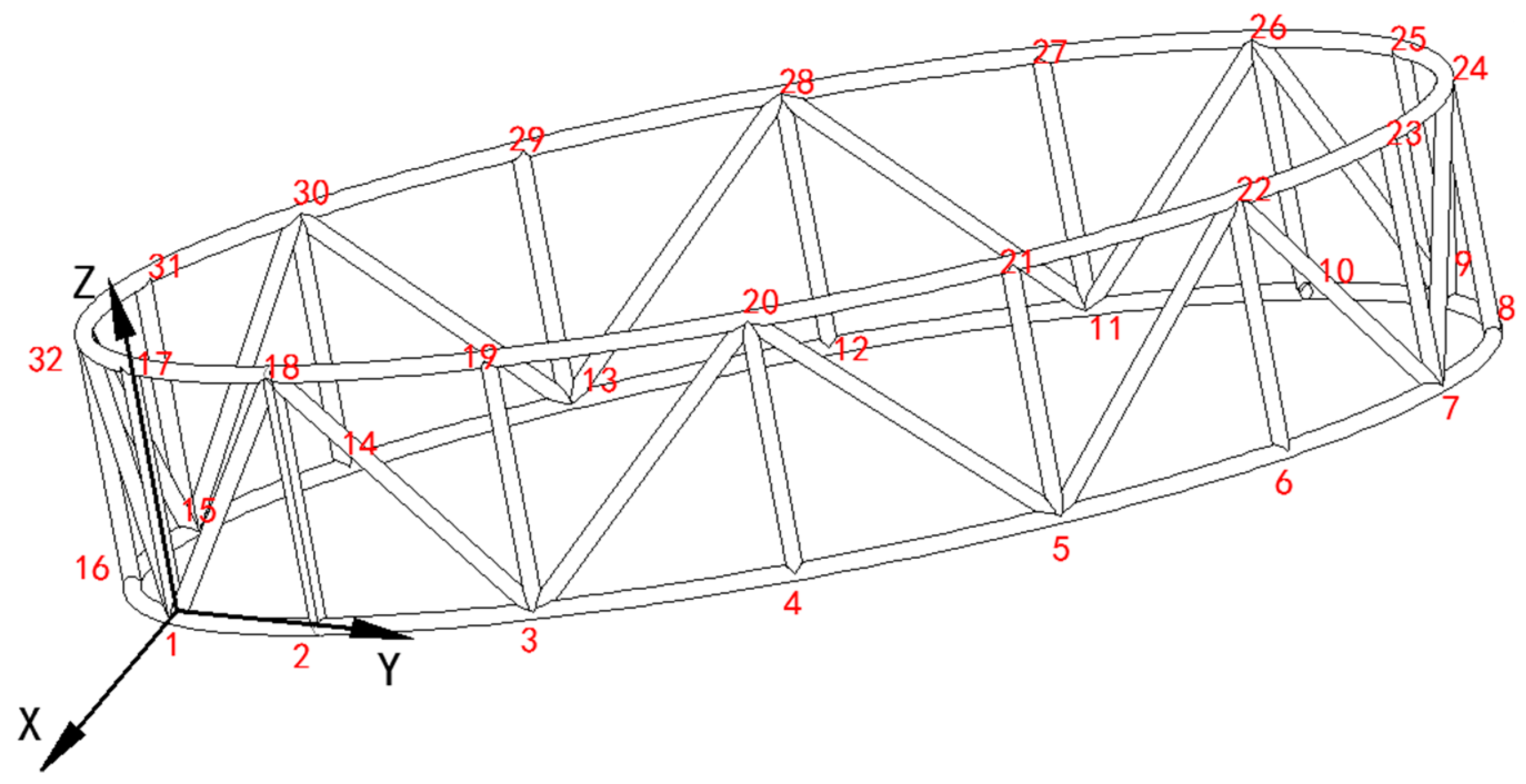
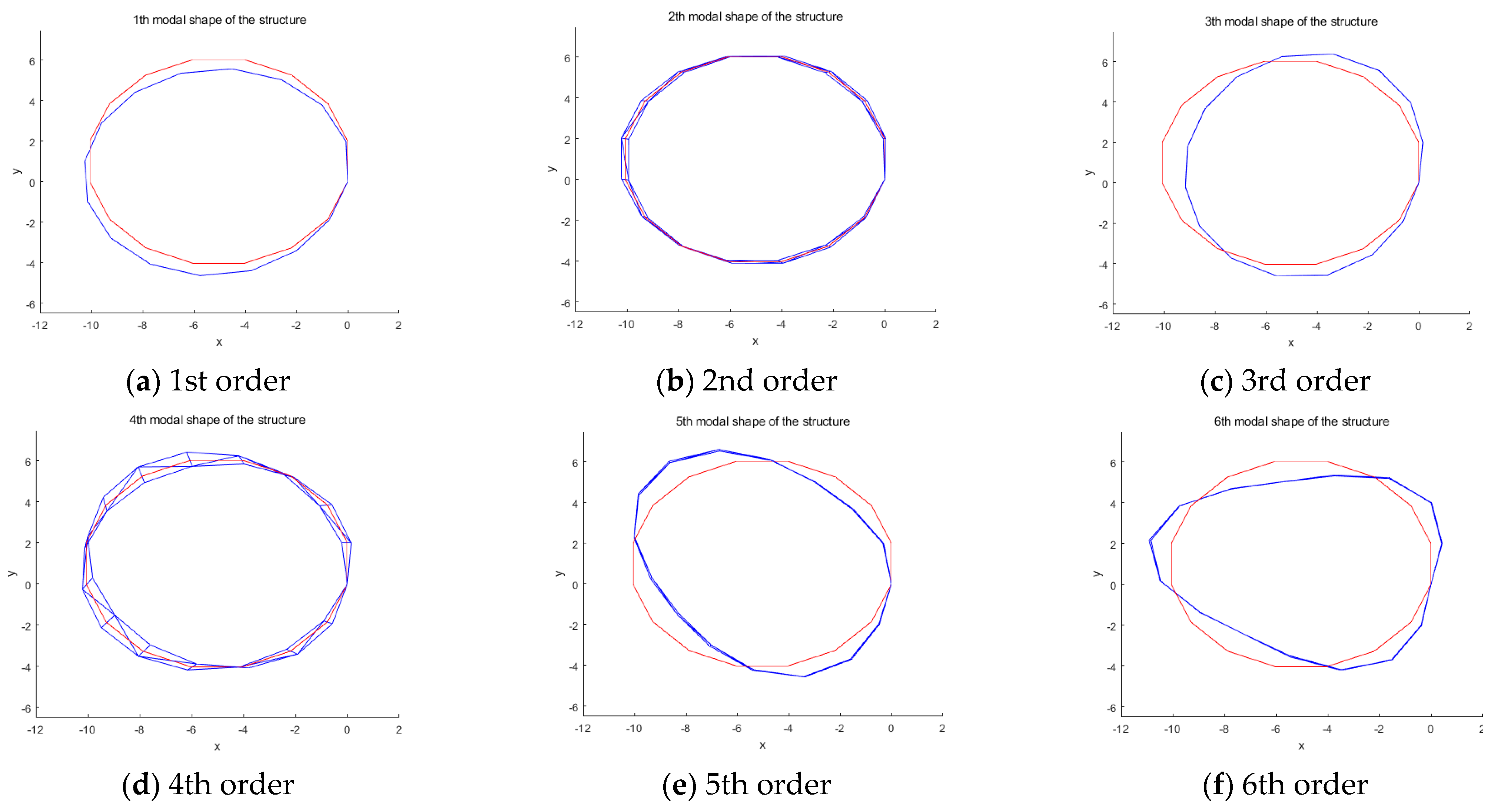
3.1. Modal and Frequency Analysis for Antenna by Finite Element Method

Generally, structures similar to plate or beam in the infinite system can be discretized by the modal shapes of the corresponding static structure. However, the structure of the hoop-truss antenna is relatively complex, and it is difficult to find the appropriate assumed modal shapes. In this study, the hoop-truss antenna is assembled by 64 thin-walled beams and 32 nodes, as shown in Figure 3. Each thin-walled beam element is regarded as a two-node element and subjected to the axial force, shear force, bending moment, and torsional moment. A finite element model is established to obtain the coordinates of the nodes, and the corresponding modal shapes matrix for the hoop-truss antenna can be found.

In our model, the length of the transverse or vertical element beam is L and the cross-section area of the beam element is A. Considering constraints between the hoop-truss antenna and the connecting boom, node 1 and node 17 are set as fixed points.

Taking the thin-walled beam element with node i and node j as an example, as shown in Figure 4, each node has six degrees of freedom including displacements u, v, and w and rotation angles of the plane cross section θ_x, θ_y, θ_z in its local coordinate system O-xyz. The element has two nodes and twelve generalized coordinates that can be expressed as:

$${\delta }_{\mathrm{local}}={\left[\begin{array}{cccccccccccc}{u}_i& v_i& w_i& {\theta }_{xi}& {\theta }_{yi}& {\theta }_{zi}& u_j& v_j& w_j& {\theta }_{xj}& {\theta }_{yj}& {\theta }_{zj}\end{array}\right]}^{\mathrm{T}}$$

(13)

and node generalized force can be expressed as:

$$P_{\mathrm{local}}={\left[\begin{array}{cccccccccccc}{U}_i& V_i& W_i& M_{xi}& M_{yi}& M_{zi}& U_j& V_j& W_j& M_{xj}& M_{yj}& M_{zj}\end{array}\right]}^{\mathrm{T}}$$

(14)

in which U denotes the axial force, V, W respectively denote the sheer forces in x-z plane and x-y plane, M_x denotes the torque, and M_y and M_z denote the bending moments in x-z plane and x-y plane, respectively.

Neglecting the internal damping and the microgravity of space, the equations of motion for the antenna in the global coordinate system O_b-X_bY_bZ_b are given by:

$$M\ddot{\mathsf{\delta }}+K\mathsf{\delta }=P$$

(15)

where δ is the nodal displacement vector, M is the mass matrix, K is the stiffness matrix in the global coordinate system, and:

$$K={\lambda }^{\mathrm{T}}{K}_{\mathrm{local}}\lambda ,M={\lambda }^{\mathrm{T}}{M}_{\mathrm{local}}\lambda ,P={\lambda }^{\mathrm{T}}{P}_{\mathrm{local}},\delta =\lambda {\delta }_{\mathrm{local}}$$

(16)

in which M_local and K_local are the mass matrix and the stiffness matrix in the local coordinate system which are both 12 × 12. λ is the transformation matrix between the local coordinate system and the global coordinate system. The detailed explanations for Equations (15) and (16) and the expressions for K, M, P, λ can be found in reference [17].

The parameters of the hoop-truss antenna are listed in

Table 1. The parameters of the hoop-truss antenna.

E (Pa)	Poisson’s Ratio	ρ (kg/m3)	L (m)	A (m2)	J (m4)
2.1 × 1011	0.3	7860	2	1.2 × 10−5	1.1 × 10−9

. Since the beam is where node 1 and node 17 are fixed, all the degrees of freedom of node 1 and node 17 are set as 0 during calculation in this study. Without considering the forces P, based on Equation (15), the natural frequencies can be obtained by solving its eigen equation and listed in

Table 2. The frequencies of hoop-truss antenna obtained by Equation (15) method and Multiphysics FEA.

Natural Frequency	1st Order Q1	2nd Order Q2	3rd Order Q3	4th Order Q4	5th Order Q5	6th Order Q6
Results by Equation (15)	0.0956	0.1450	0.2656	0.5135	0.5621	0.9534
Multiphysics FEA	0.0945	0.1453	0.2660	0.5151	0.5632	0.9541
Relative error	1.15%	0.2%	0.15%	0.3%	0.2%	1.0%
Vibration type	Roll	Bend	Respiration	Torsion	Respiration	Respiration

. For comparison, the natural frequencies obtained by Multiphysics FEA are also given in Table 2. It can be found that the relative error of the first eight orders of natural frequencies between the two methods is less than 1%.

In addition, according to the geometrical relationship between element beams of the hoop-truss antenna, the initial coordinate of each node is set. The vibration mode shapes of the hoop-truss antenna can be found by solving the nodal displacements δ in Equation (15). In other words, the modal vector Q_i representing the ith modal shape of the structure can be obtained by the ith order nodal displacements, which is 1 × 96. The corresponding three-dimensional nodal displacements are listed in

Table 3. Modal statistics of hoop-truss antenna.

No- De	1st Order Q1	2nd Order Q2	3rd Order Q3	4th Order Q4	5th Order Q5	6th Order Q6
1	0	0	0	0	0	0
	0	0	0	0	0	0
	0	0	0	0	0	0
2	−0.0675	0.0487	0.1634	0.1483	−0.3308	0.4136
	−3.3781 × 10−7	−6.9022 × 10−8	−9.9813 × 10−7	−6.1993 × 10−5	1.2884 × 10−5	−1.1044 × 10−5
	−2.0289 × 10−7	−1.0936 × 10−5	−1.4794 × 10−6	1.1054 × 10−4	1.9173 × 10−5	−7.9880 × 10−6
⋮		⋮	⋮	⋮	⋮	⋮
32	−6.2998 × 10−5	−0.0212	6.7216 × 10−5	0.0650	−0.0055	0.0047
	0.0001	−0.0488	0.0005	0.1555	−0.0128	0.01150
	0.0648	−0.0336	0.141	0.1031	0.2396	0.3014

and the corresponding modal shapes for the first six orders are shown in Figure 5.

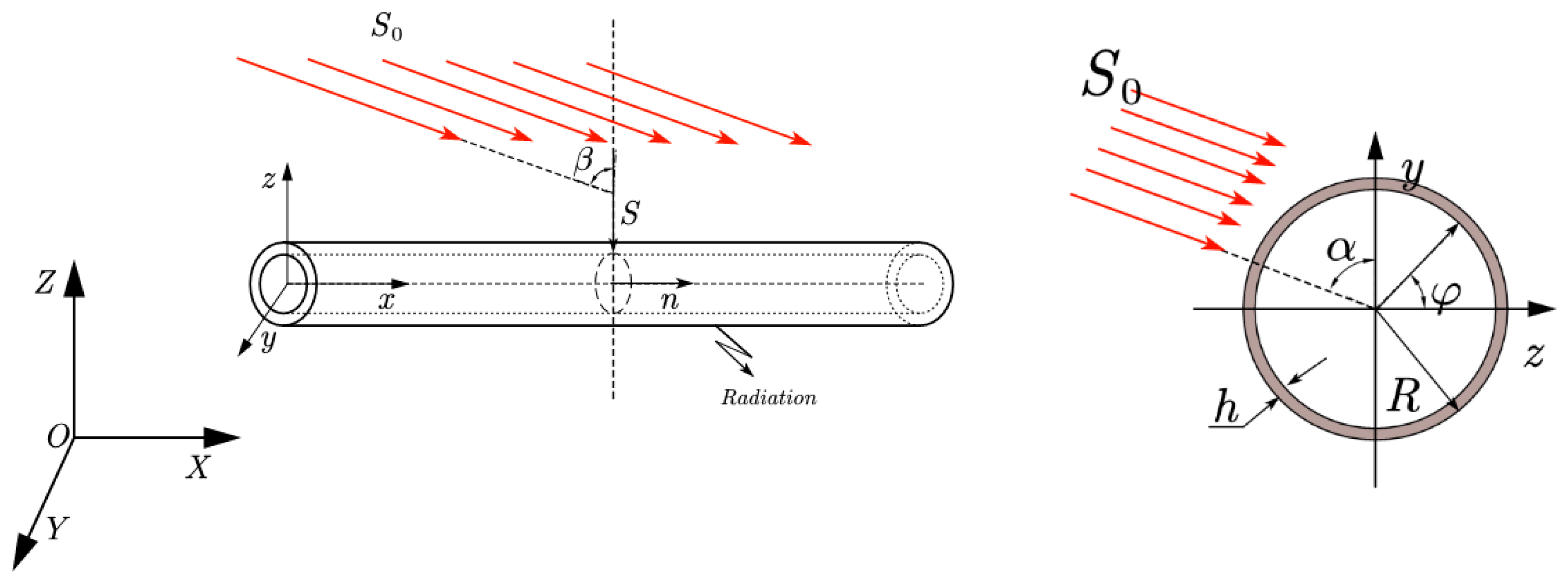
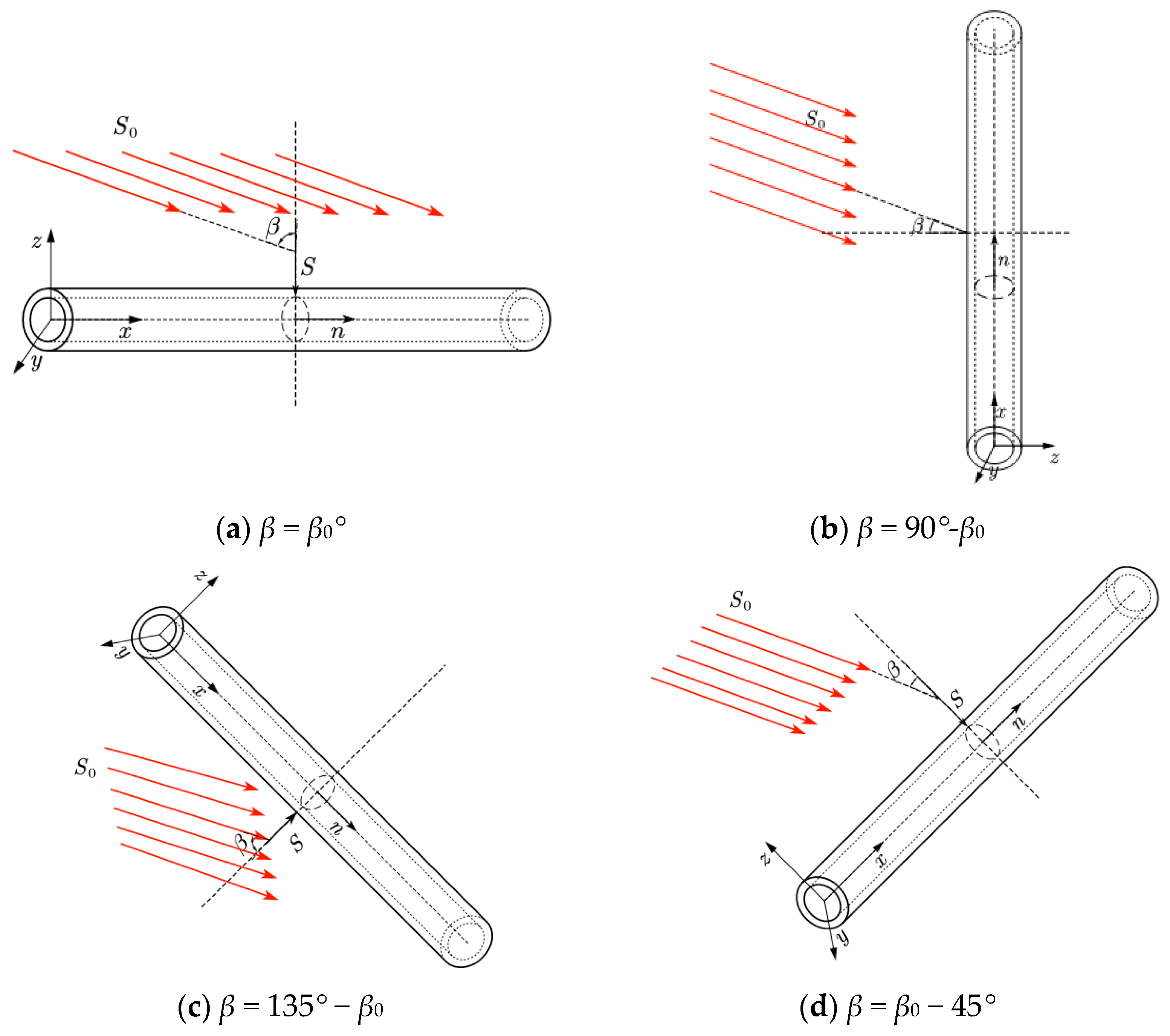
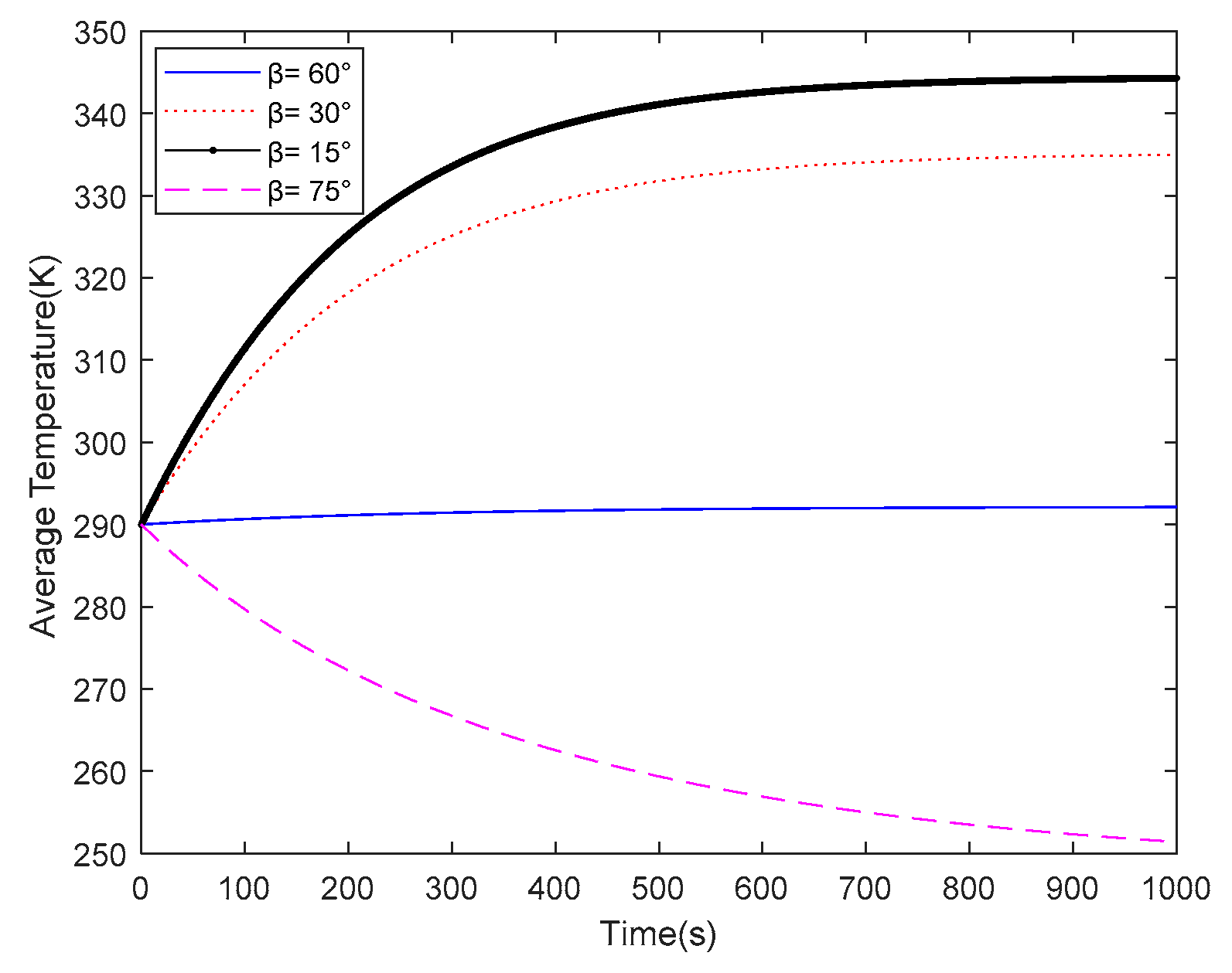
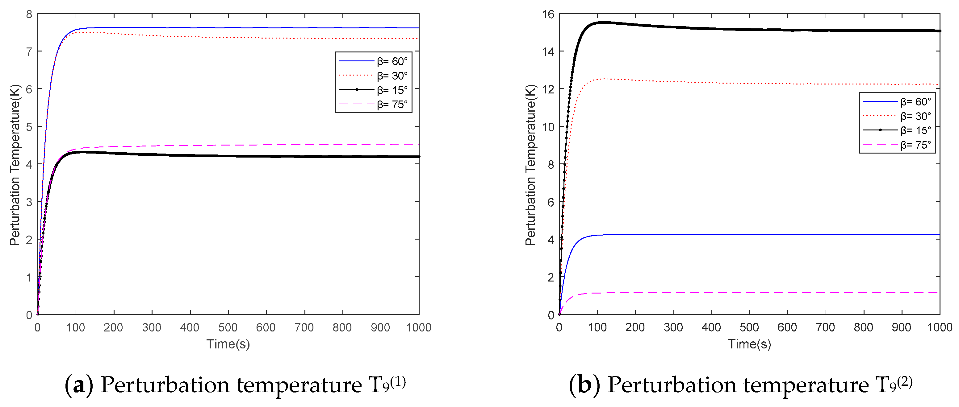
3.2. Thermal Analysis

Since the heat transfer function is dependent on the local deformation of the structure, the classical FEM cannot treat this type of coupling well. The proposed method in this section combines the FEM and generalized method to take into account the local deformation-dependent heat transfer effect.

The beams of the hoop-truss antenna structure are simplified as thin-walled beams as shown in Figure 6. The beams are subjected to solar flux S₀ as the hoop-truss antenna exits the Earth’s shadow. For the thin-walled beams that are subject to solar radiation in the space, their exterior surface would absorb solar radiation heat flux, at the same time, the outward radiation heat flux occurs to the space at the temperature of 0 K, and the heat convection to the space is neglected due to the vacuum and low pressure.

According to Fourier’s law for the heat conduction and neglecting the temperature variation across the wall thickness. The transient heat transfer in the thin-walled beams of the hoop-truss is given by:

$$\frac{\partial T}{\partial t}-\frac{k_x}{\rho c}\frac{{\partial }^{2}T}{\partial x^2}-\frac{k_{\phi }}{\rho c{R}^2}\frac{{\partial }^{2}T}{\partial {\phi }^2}+\frac{\sigma \epsilon }{\rho ch}{T}^4=\frac{{\alpha }_s{S}_0\cos \beta }{\rho ch}\varsigma \cos \phi$$

(17)

where T is the temperate, c is the specific heat, k_x and k_φ are respectively the thermal conductivity along axis-direction x and circumferential direction φ, R is the radius of the beam, σ is the Stefan–Boltzmann constant, ε is the surface emissivity, α_s is the surface absorptivity, and h is the thickness of the wall. The heat flux S is the projection of solar flux S₀, which is always perpendicular to the normal direction n of the cross section, as shown in Figure 6. The α is the angle between solar flux S₀ and the z direction of the cross section, which is different for each element beam as shown in Figure 6. The parameter ς is introduced to indicate whether the beam surface is exposed to solar flux.

$$\varsigma =\{\begin{array}{ll}1,& \frac{\pi }{2}-\alpha <\phi <\frac{3\pi }{2}-\alpha \\ 0,& -\frac{\pi }{2}-\alpha <\phi <\frac{\pi }{2}-\alpha \end{array}$$

(18)

Particularly, in our study, the solar radiation angle β for different beams can be divided into four types according to the angle between solar radiation S₀ and the perpendicular direction to the normal direction n. When the solar radiation angle of the horizontal beam β is equal to β₀, they are β = β₀°, β = 90° − β₀, β = 135° − β₀, β = β₀ − 45°, as shown in Figure 7.

By following the steps in reference [20], the thermal load vectors on the thin-walled beam caused by thermal shock can be expressed as:

$$F_T=EA{\alpha }_T\left(\frac{{\overline{T}}_i+{\overline{T}}_j}{2}-T_0\right){\left[\begin{array}{cccccccccccc}-1& 0& 0& 0& 0& 0& 1& 0& 0& 0& 0& 0\end{array}\right]}^{\mathrm{T}}$$

(19)

$$M_T=\frac{EI{\alpha }_T}{Rl}{\left[\begin{array}{cccccccccccc}0& 0& 0& 0& -l{T}_i^{(1)}& l{T}_i^{(2)}& 1& 0& 0& 0& l{T}_j^{(1)}& -l{T}_j^{(2)}\end{array}\right]}^{\mathrm{T}}$$

(20)

where node i and node j are in the same beam,${\overline{T}}_i$ and ${\overline{T}}_i$ are defined as the average temperatures for node i and j, and T_i⁽¹⁾ and T_i⁽²⁾ are the perturbation temperatures on the cross section. T₀ is the initial temperature. The α_T is the coefficient of thermal expansion. The correspondingly thermal-induced generalized force P_local for node i and node j is derived as:

$$P_{\mathrm{local}}=F_T+M_T$$

(21)

In Equation (21), the first six elements represent the generalized forces of node i, and the rest of the elements represent the generalized forces of node j. Then, based on Equations (15) and (16), the thermal-induced vibration response in the general coordinate system for the antenna can be obtained.

To explain the causes of thermally induced dynamical behaviors of the antenna, thermal–structural dynamics of the single hoop-truss are analyzed. All the parameters used in the simulations are listed in

Table 4. Thermal structure data of spatial beam thin-walled beam.

Parameter	Value	Units	Parameter	Value	Units
E	2.1 × 1011	Pa	kx	16.6	W/m·K
ν	0.3	-	kφ	16.6	W/m·K
ρ	7860	kg/m3	ε	0.13	-
c	502	J/kg·K	αs	0.6	-
l	2	m	αT	1 × 10−8	1/K
R	0.009733	m	S0	1350	W/m2
r	0.00953	m	β0	60	degree

.

Considering the solar radiation angle of the horizontal beam is β = β₀ = 60°, the corresponding solar radiation angle for vertical beam, left inclined beam, and right inclined beam are β = 30°, β = 15°, and β = 75°, respectively. Figure 8 and Figure 9 respectively show the thermal response of the node’s average temperatures and perturbation temperatures for beams with different solar radiation angles.

Taking the horizontal beam that β = 60° with node 9 and node 25 as an example, the thermal responses of average temperature ${\overline{T}}_9$ for node 9 denoted as the blue line are increased until they reach their steady-state values, as shown in Figure 8. The perturbation temperatures T₉⁽¹⁾, T₉⁽²⁾ are shown in Figure 9a,b, which are also increased with time until reaching their steady-state values. It can be found that the perturbation temperature responses are much faster than the average temperature responses which are stable in 100 s. The temperature responses for node 25 can be performed in a similar way.

For the beams with solar radiation angles, β = 30° and β = 15°, the trends for the responses are the same as the horizontal beam. The less the solar radiation angle is, the larger the steady-state average temperature is. This phenomenon is quite understandable since a lower value β on the right side of Equation (17) can result in a lower value of cosβ. For the right inclined beam with solar radiation angle β = 75°, the trend for the average temperature response is quite opposite to the response of the horizontal beam due to the heat flux absorbed being less than that emitted from the surface radiation in this condition. The simulation results for the right inclined beam agree well with Figure 10a in reference [3] for a single boom.

Based on Equation (21), the generalized force P_local of each beam is obtained. Then, the total generalized force P of the whole antenna can be obtained by superposition according to the coordinates of nodes. By substituting P into Equation (15), the displacement and rotation response of each node under thermal shock can be analyzed.

The displacements of the representative six nodes including the starting nodes 1 and 17, middle nodes 9 and 25, and the farthest nodes 5 and 21 are shown in Figure 10, Figure 11 and Figure 12. Since node 1 and node 17 are fixed to the connecting boom, there are no displacements for these two nodes. Figure 10 shows the dynamic response of node 5 in the global coordinate system. It can be found that the thermal deformations are dominated and the thermal vibrations are not obvious. Among three directions, the thermal deformation in the y-direction is large, while the vibration in the z-direction is the most significant. The angular displacement is mainly shown in the x-axis direction, while the angular vibration in θ_y-direction is the most noteworthy. The steady deformations are about −0.027 m, −0.044 m, −0.008 m, −0.0038 deg, −0.008 deg, and 0.015 deg. Similar conclusions can be found for node 21. For the sake of simplicity, the displacements of nodes 1, 17, and 21 are not provided in this paper redundantly.

The dynamic responses for the farthest nodes 9 and 25 are shown in Figure 11 and Figure 12, respectively. In Figure 11, it is found that similar to node 5, the thermal deformations in six dimensions are still more severe than vibrations, and the vibration in z-direction and θ_y-direction are the most significant. In addition, the deformations in x-direction, y-direction, θ_x-direction, and θ_w-direction are almost the same as those for node 5, while the deformations in the z-direction and θ_y-direction grow significantly. The steady deformations are about −0.027 m, −0.044 m, −0.3 m, −0.0038 deg, −0.05 deg, and 0.015 deg. The farther the node is from the fixed rod, the greater the displacements can be.

The simulations in this subsection provide basic information for thermal-induced vibration responses, which will be used as a comparison for the coupling condition in Section 4.

4. Coupled Dynamic and Control for Thermally Induced Vibration and Attitude Motion

With the modal matrix Q obtained in Section 3, we can further analyze the coupling rotational equations of motion and translational equations of motion, and design the attitude control law to achieve stable on-orbit operation.

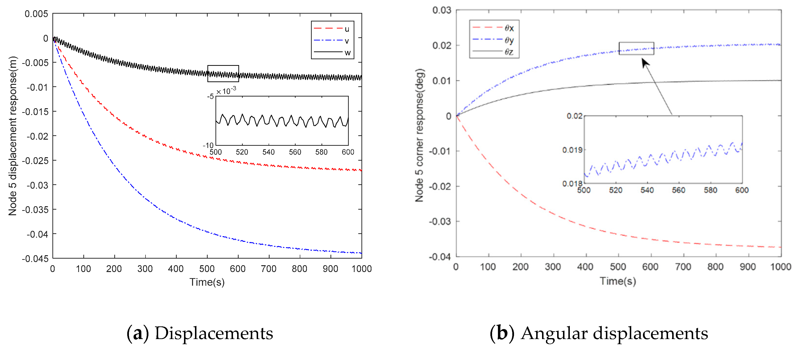
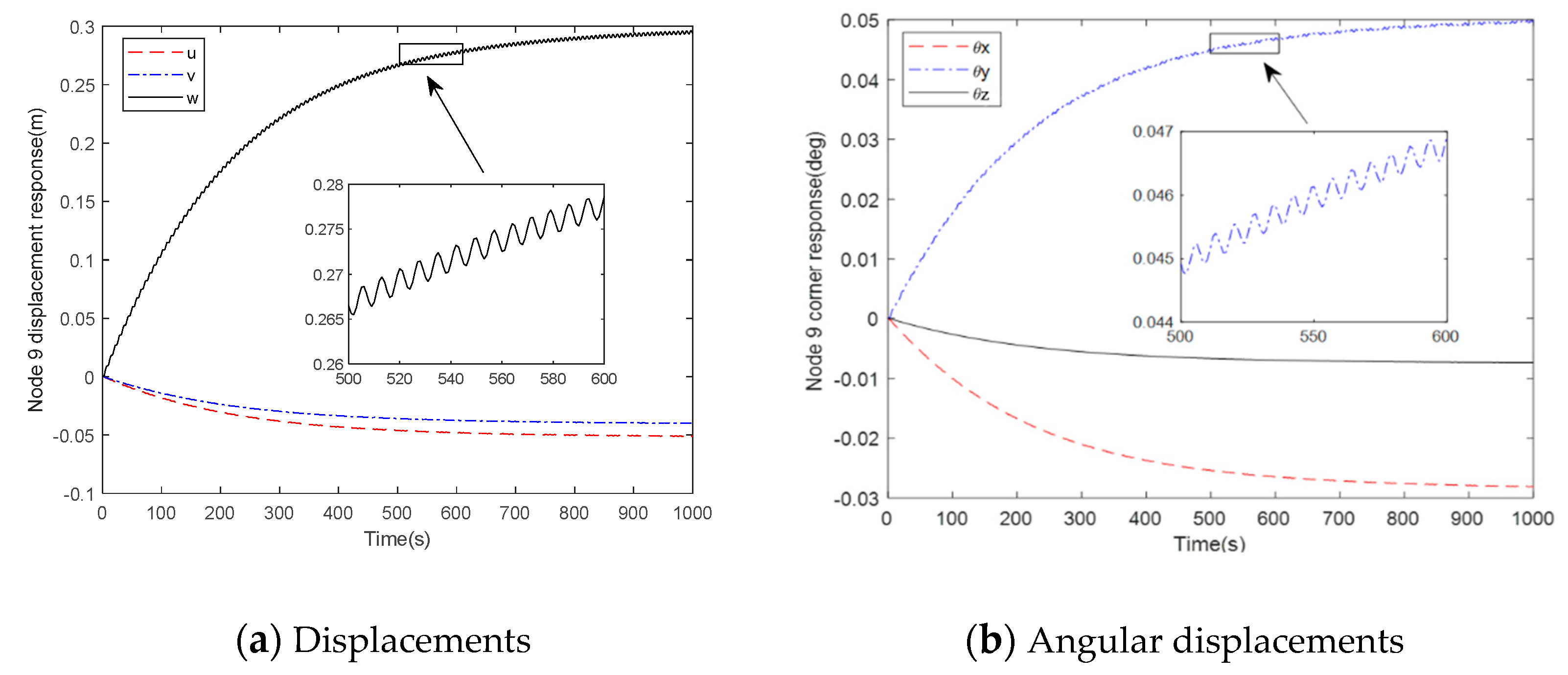
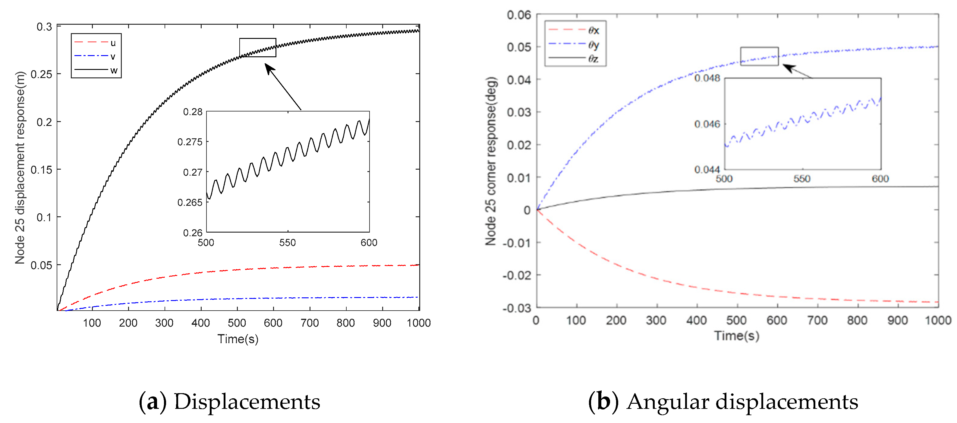
4.1. Dynamic Response of Rigid-Flexible Coupled Structure

Generally, the communication satellite moves in a geosynchronous orbit and the antenna rotates uniformly around the central rigid body, we consider the ${\ddot{R}}_1$ and ${\dot{\omega }}_a$ both equal to zeroes.

By rearranging Equations (10) and (11) and omitting higher-order small variables, the coupling equation of motion of the antenna’s vibration and the satellite’s attitude motion can be expressed as:

$$\left(I_b+I_{ab}^b\right)\dot{\omega }=-\left(I_{\omega }+I_{\mathsf{\Omega }ab}^b\right)\mathsf{\omega }+H_{ab}{P}_a{\ddot{\eta }}_a+T_c$$

(22)

$$M_a{P}_a{\ddot{\eta }}_a+K_a{\eta }_a-\left(S_b+S_{ba}\right)A_{ab}\dot{\omega }-{\left(A_{ab}\omega \right)}^{\mathrm{X}}\left(S_b+S_{ba}\right)A_{ab}\mathsf{\omega }=F$$

(23)

where thermal load F acting on the antenna can be obtained by the modal matrix Q and the thermal moment M_T in Section 3. In the following part, we consider that the η_a = [η₁, η₂, η₃]^T which are the first three order modal coordinates.

It is clear that the thermal-induced vibration of the antenna can affect the stability of the spacecraft attitude; thus, the attitude needs to be controlled.

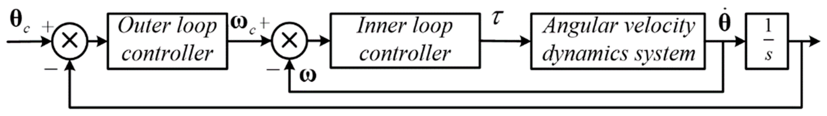
4.2. Attitude Controller Design Based on Slide Mode Control Theory

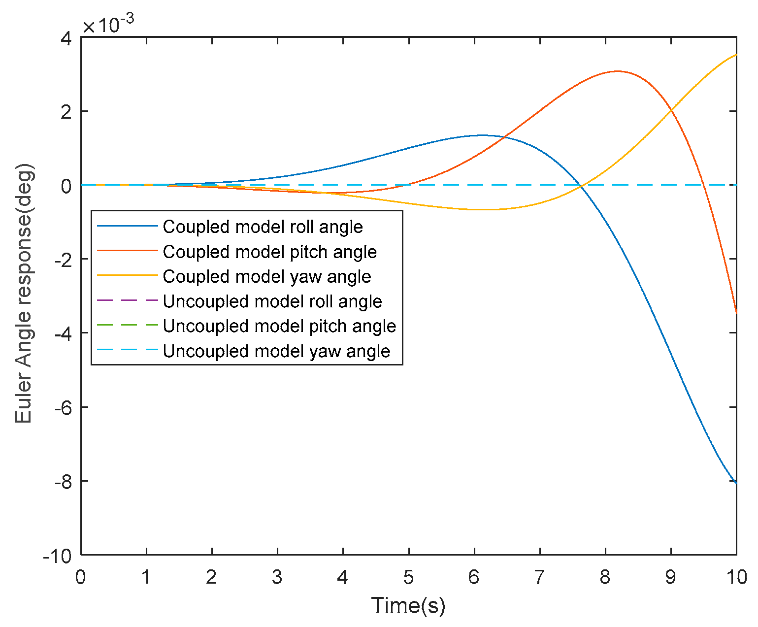
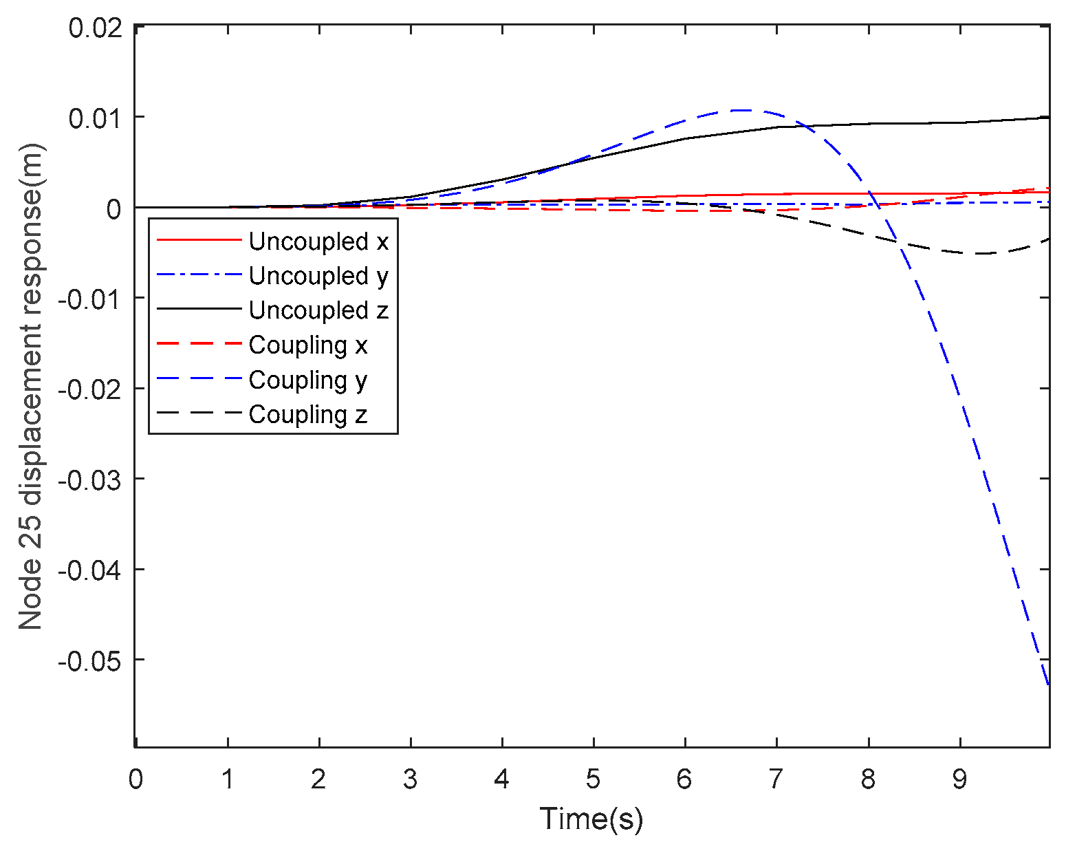
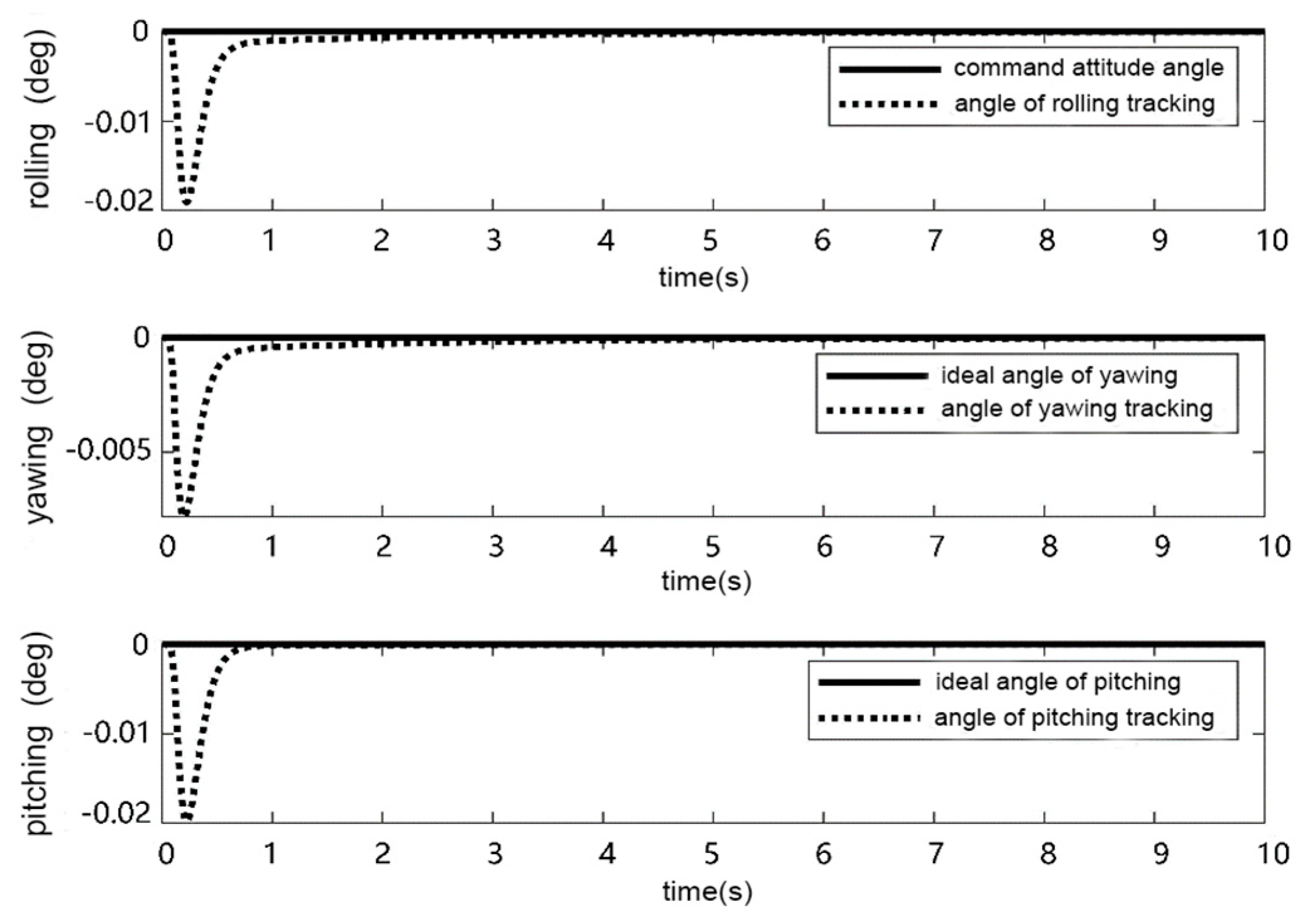
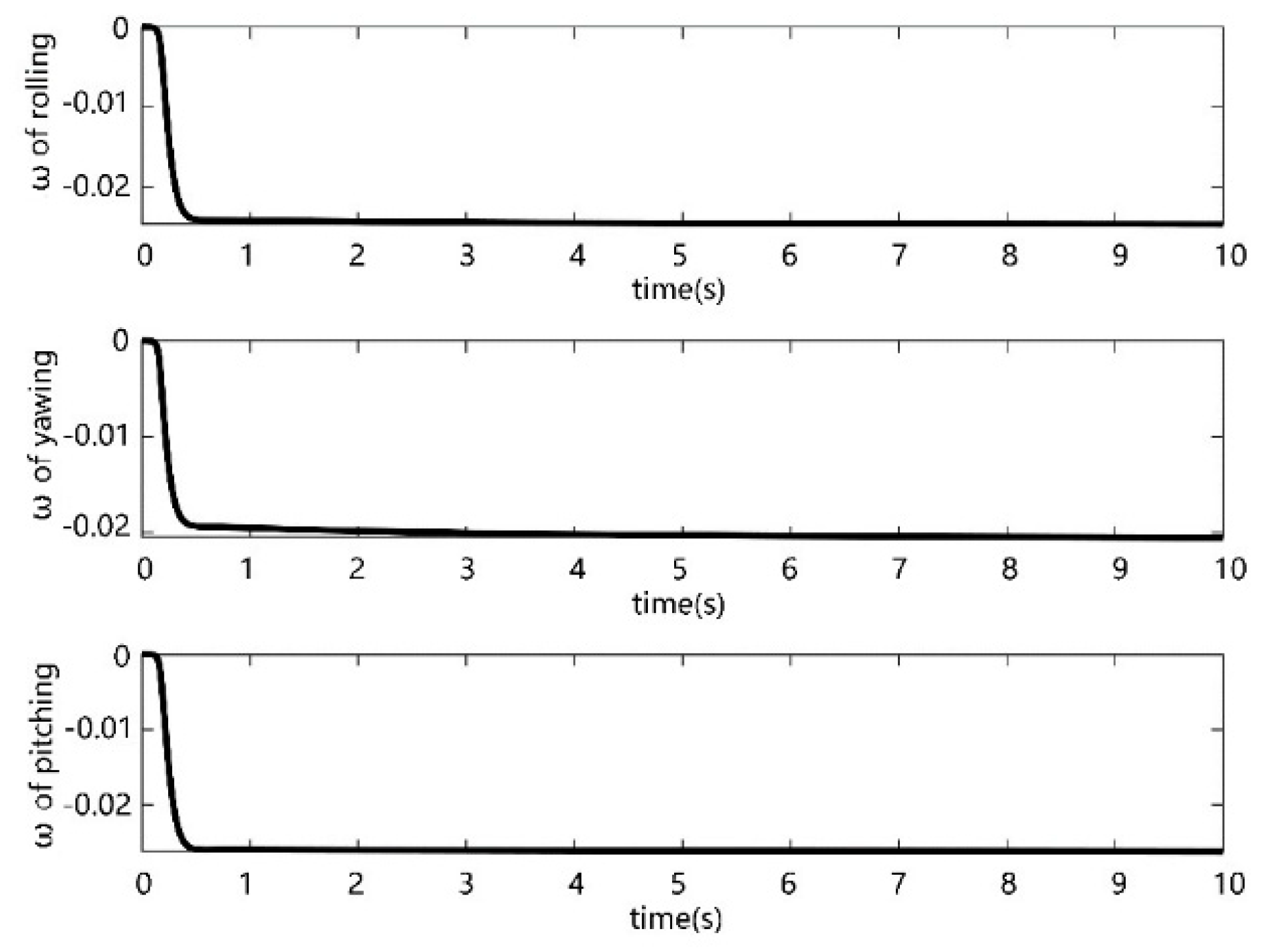
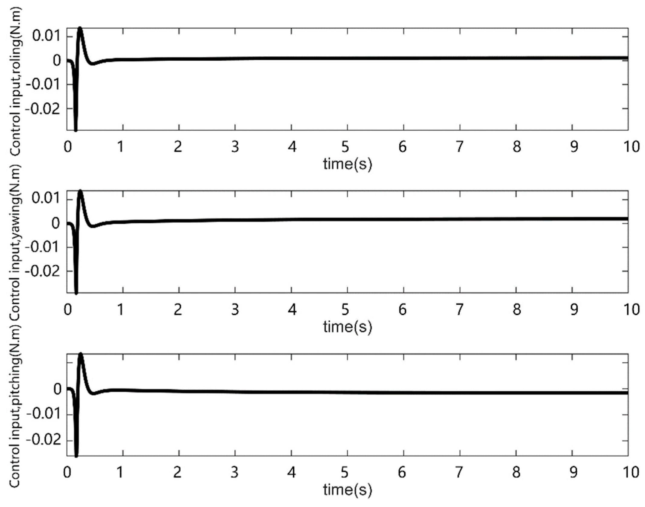
Sliding mode control is a practical method that can overcome system uncertainty and has robustness to disturbance and unmodeled dynamics. As for spacecraft equipped with large antennas, the divergence caused by the uncertainty of thermally induced vibration and the system nonlinearity can be suppressed with sliding mode control. It is also a relatively simple algorithm with high robustness to nonlinearity and is easy to realize in satellite. Examples of applications of sliding mode control on large spacecrafts can be found in reference [31,32,33]. By substituting Equation (23) into Equation (22), the dynamic equation of the attitude motion can be expressed as:

$$J\dot{\mathsf{\omega }}=-\Omega J\omega +T_c+D$$

(24)

where T_c denotes the external control torque, and:

$$J=\left(I_b+I_{ab}^b-H_{ab}{P}_a{\left(M_a{P}_a\right)}^{-1}\left(S_b+S_{ba}\right)A_{ab}\right)$$

(25)

and Ω = [ω]^X, D denotes disturbances:

$$D=H_{ab}{P}_a{\left(M_a{P}_a\right)}^{-1}F-H_{ab}{P}_a{\left(M_a{P}_a\right)}^{-1}{K}_a{\eta }_a$$

(26)

By designing the external control torque T_c, the system output can follow the ideal attitude angular velocity ω_c.

In addition, based on the attitude dynamics, we can obtain that:

$$\dot{\theta }=R\left(\phi , \theta , \psi \right)\mathsf{\omega }$$

(27)

where θ = [φ θ ψ]^T, the φ, θ, ψ are the roll, pitch, and yaw angle, respectively, and

$$R\left(\phi , \theta , \psi \right)=\left[\begin{array}{ccc}\cos \theta & 0& -\cos \phi \sin \theta \\ 0& 1& \sin \phi \\ \sin \theta & 0& \cos \phi \cos \theta \end{array}\right]$$

(28)

The double-loop sliding mode variable structure control method is adopted, which is shown in Figure 13. The control system is composed of the inner angular velocity loop and the outer angular loop. The switching function can be designed by using the integral sliding mode control. The outer loop is mainly used to design attitude angular velocity command ω_c. The inner loop gives out the torques commands of the satellites to follow the command attitude angular velocity ω_c through the sliding mode control law.

Defining θ_e = θ_c − θ where θ_c is the command attitude angle and the θ is the real attitude angle, the outer loop sliding model surface is defined as follows:

$$s_w={\theta }_e+K_1{\displaystyle {\int }_0^t{\theta }_{e}dt}$$

(29)

where K₁ = diag{k₁₁, k₁₂, k₁₃} > 0 is the gain matrix.

$${\dot{s}}_w={\dot{\theta }}_e+K_1{\theta }_e={\dot{\theta }}_c-\dot{\theta }+K_1{\theta }_e={\dot{\theta }}_c-R{\omega }_c+R{\omega }_e+K_1{\theta }_e$$

(30)

The ω_c needs to be designed as a differentiable form as:

$${\omega }_c=R^{-1}\left({\dot{\theta }}_c+K_1{\theta }_e\right)+R^{-1}{\rho }_1{s}_w\hspace{1em}\left({\rho }_1>0\right)$$

(31)

The Lyapunov method is used to determine the stability of the system. A generalized Lyapunov function, which characterizes the motion of the state trajectory to the sliding surface, is defined in terms of the sliding surface. For each chosen switched control structure, the control law is designed so that the derivative of the Lyapunov function is negative definite, thus guaranteeing the motion of the state trajectory to the surface. The Lyapunov function for the outer loop is chosen to be:

$$V_1=\frac{1}{2}{s}_w^T{s}_w$$

(32)

The derivative of the Lyapunov function can be given by:

$$\begin{array}{ll}{\dot{V}}_1& =s_w^T{\dot{s}}_w=s_w^T\left({\dot{\theta }}_c-\dot{\theta }+K_1{\theta }_e\right)\\ & =s_w^T\left\{{\dot{\theta }}_c-R\left[R^{-1}\left({\dot{\theta }}_c+K_1{\theta }_e\right)+R^{-1}{\rho }_1{s}_w\right]+R{\omega }_e+K_1{\theta }_e\right\}\\ & =-{\rho }_1{\Vert s_w\Vert }^2+s_w^{T}R{\omega }_e\end{array}$$

(33)

It can be noticed that error ω_e in Equation (33) needs to be small enough to ensure the derivative of the Lyapunov function is negative ${\dot{V}}_1$ ≤ 0, which requires fast convergence of the inner loop.

Similarly, the integral sliding mode surface is used to design the inner loop, that is:

$$s_n={\omega }_e+K_2{\displaystyle {\int }_0^t{\omega }_{e}dt}$$

(34)

where K₂ = diag{k₂₁, k₂₂, k₂₃} > 0 is gain matrices. Considering Equation (24), one can obtain:

$${\dot{s}}_n={\dot{\omega }}_e+K_2{\omega }_e={\dot{\omega }}_c+J_{}^{-1}\left(-\Omega J\omega +W+D\right)+K_2{\omega }_e$$

(35)

The inner loop control law is designed as follows:

$$T_c=\Omega J\omega +J\left({\dot{\omega }}_c+K_2{\omega }_e\right)+{\rho }_2\mathrm{SIGN}\left(s_n\right)+k{s}_n$$

(36)

where ${\rho }_2>\max \left|D_i\right|$, $k=\left[\begin{array}{cc}k& 0\\ 0& k\end{array}\right]>0$. Then,

$${\dot{s}}_n=-J_{}^{-1}\left({\rho }_2\mathrm{SIGN}\left(s_n\right)+k{s}_n+D\right)$$

(37)

Consider the Lyapunov function as follows:

$$V_2=\frac{1}{2}{s}_n^T{J}_w{s}_n$$

(38)

The derivative of the Lyapunov function can be given by:

$${\dot{V}}_2=s_n^T{J}_w{\dot{s}}_n=-{\rho }_2{\displaystyle \sum _{i=1}^3\left|s_n\right|}-s_n^{T}D-k{\Vert s_n\Vert }^2\le -k{\Vert s_n\Vert }^2$$

(39)

We can conclude from Equation (39) that ${\dot{V}}_2$ ≤ V₂, and V₂ ≤ e^-t. When t→∞, V₂ convergences. Thus, the system is asymptotically stable.

4.3. Simulations

We consider the mass of the central rigid body of the satellite M_b to be equal to 100 kg. Based on the parameters in Table 4, the mass of the satellite antenna M_a can be obtained as 12.3595 kg. Momentum wheels installed along body axes serve as the attitude actuator whose maximum torque output is 0.03 Nm. The remaining parameters used in Equation (24) can also be obtained by the parameters in Table 4.

Based on Equations (22) and (23) and considering the initial attitude angle vector θ and initial angular velocity ω are both 0, the angular responses of the rigid-flexible coupled system and the single rigid body without control are given in Figure 14. It can be seen from Figure 14 that without the vibration, the attitude angles maintain zeros, and the thermal induced vibrations have great influence on the attitude angles which cause the attitude motion to diverge rapidly. In return, the variations of attitude angles also cause the model coordinates η_a to diverge which finally results in the large displacements for the node coordinates. A simple example of the displacements for node 25 is shown in Figure 15. The red line, black line, and blue dash-dotted line denote the uncoupled responses which are adopted from Figure 12 and shown as a comparison. The red, black, and blue dash lines denote the coupled responses based on Equations (22) and (23). Therefore, it is necessary to consider a control law to ensure a stable operation in space.

Based on the control law for external moment T_c in Equation (36) and assuming the command attitude angle θ_c = 0, we can choose the control parameters to guarantee the convergence of the system. To verify the asymptotic stability of the controller, the optimization of the parameters was not included in this paper and we simply choose a feasible solution of the control parameter. The outer loop control coefficients ρ₁ = 3, K₁ = diag{10,10,10}, inner loop control coefficients ρ₂ = 3, K₂ = diag{100,100,100}, k = diag{300,300,300}, and the controlled results for attitude angles, angular velocities, and control moments are shown in Figure 16, Figure 17 and Figure 18, respectively. It is found that the attitude angular velocity commands of the three axes gave out immediately along with the control commands and the bias of the attitude angle caused by the thermal-induced load can be restrained in short time under the action of the control torques. The stabilization time is within 1 s, and the control torque is within 0.03 Nm, which can fit the actual constraint requirements of the onboard actuators. During the process, the attitude angles slowly coincide with the command attitude angle θ_c. The angular biases of three axes are within 1.313 × 10⁻³ deg, 6.569 × 10⁻⁴ deg, and 4.055 × 10⁻⁴ deg, respectively, at 1 s. The variations of the angular biases are listed in

Table 5. Angular biases.

Time/s	Rolling Bias/Deg	Yawing Bias/Deg	Pitching Bias/Deg
0.5	3.130 × 10−3	1.674 × 10−3	4.298 × 10−3
0.65	2.189 × 10−3	9.872 × 10−4	7.625 × 10−4
1	1.313 × 10−3	6.569 × 10−4	4.055 × 10−4
2	7.461 × 10−4	3.649 × 10−4	3.892 × 10−4
7	5.087 × 10−5	4.853 × 10−5	5.472 × 10−5

. It is found that after 1 s, the biases for three axes drop dramatically to the order of 10⁻⁴, and the biases will keep dropping to the order of 10⁻⁵ at 7 s. The angular velocity biases of the three axes are with 3.840 × 10⁻³ deg/s, 3.959 × 10⁻³ deg/s, and 5.570 × 10⁻³ deg/s from 0.5 s. Similarly, the variations of the angular velocity biases are listed in

Table 6. Angular velocity biases.

Time/s	Rolling Bias/Deg	Yawing Bias/Deg	Pitching Bias/Deg
0.5	3.840 × 10−3	3.959 × 10−3	5.570 × 10−3
0.7	2.647 × 10−3	2.617 × 10−3	4.496 × 10−3
0.85	2.348 × 10−3	2.348 × 10−3	4.228 × 10−3
1	2.319 × 10−3	2.319 × 10−3	4.198 × 10−3

.

The simulation results show the effectiveness of the proposed controller which has the advantages of fast-tracking response, short adjustment time, and good convergence. The controller can accurately track the attitude angles and restrain the thermal vibrations of the spacecraft.

5. Conclusions

This study focuses on thermally induced dynamical behaviors and control strategy of the satellite’s attitude motion and hoop-truss antenna’s vibration due to thermal shock from solar flux.

The rigid-flexible coupled dynamic model of spacecraft is derived by using the law of conservation of momentum and angular momentum. An analytical approach based on a finite element method is developed for thermal–structural dynamic analysis of the antenna. The modal shapes and natural frequencies of antenna obtained from the finite element method and the results obtained from Multiphysics FEA verify the proposed method. The numerical results indicate that the thermally induced deformations and vibrations of the antenna are mainly caused by average temperature, rather than perturbation temperatures.

The coupled responses demonstrate that the vibrations have significant influences on the attitude motion; the attitude motions also in turn affect the vibrations. The double-loop sliding mode variable structure control method is adopted to reduce the vibration while maintaining the attitude. The control system is composed of the inner angular velocity loop and the outer angular loop. The simulation results show the controller can accurately track the attitude angles and restrain the thermal vibrations efficiently.

References

1. Gasbarri, P.; Monti, R.; De Angelis, C.; Sabatini, M. Effects of uncertainties and flexible dynamic contributions on the control of a spacecraft full-coupled model. Acta Astronaut. 2014, 94, 515–526. [Google Scholar] [CrossRef]
2. Thornton, E.A.; Kim, Y.A. Thermally-induced bending vibrations of a flexible rolled-up solar-array. J. Spacecr. Rocket. 1993, 30, 438–448. [Google Scholar] [CrossRef]
3. Xue, M.-D.; Duan, J.; Xiang, Z.-H. Thermally-induced bending-torsion coupling vibration of large scale space structures. Comput. Mech. 2007, 40, 707–723. [Google Scholar] [CrossRef]
4. Johnston, J.D.; Thornton, E.A. Thermally induced dynamics of satellite solar panels. J. Spacecr. Rocket. 2000, 37, 604–613. [Google Scholar] [CrossRef]
5. Pelton, J.N.; Madry, S.; Camacho-Lara, S. Handbook of Satellite Applications; Springer: New York, NY, USA, 2013. [Google Scholar]
6. Xue, Y.; Li, Y.; Guang, J.; Zhang, X.; Guo, J. Small satellite remote sensing and applications—History, current and future. Int. J. Remote Sens. 2008, 29, 4339–4372. [Google Scholar] [CrossRef]
7. Liu, L.; Cao, D.; Wei, J. Rigid-flexible coupling dynamic modeling and vibration control for flexible spacecraft based on its global analytical modes. Sci. China-Technol. Sci. 2019, 62, 608–618. [Google Scholar] [CrossRef]
8. Liu, L.; Wang, X.; Sun, S.; Cao, D.; Liu, X. Dynamic characteristics of flexible spacecraft with double solar panels subjected to solar radiation. Int. J. Mech. Sci. 2019, 151, 22–32. [Google Scholar] [CrossRef]
9. Azimi, M.; Joubaneh, E.F. Dynamic modeling and vibration control of a coupled rigid-flexible high-order structural system: A comparative study. Aerosp. Sci. Technol. 2020, 102, 105875. [Google Scholar] [CrossRef]
10. Cao, Y.; Cao, D.; Huang, W. Nonlinear dynamic modeling and decoupling for rigid-flexible coupled system of spacecraft with rapid maneuver. Inst. Mech. Eng. Part C-J. Mech. Eng. Sci. 2019, 233, 4896–4913. [Google Scholar] [CrossRef]
11. Guo, X.; Yang, X.; Liu, F.; Liu, Z.; Tang, X. Dynamic analysis of the flexible hub-beam system based on rigid-flexible coupling mechanism. Inst. Mech. Eng. Part K-J. Multi-Body Dyn. 2020, 234, 536–545. [Google Scholar] [CrossRef]
12. Axisa, F. Modeling of Mechanical Systems—Structural Elements; Elsevier: Amsterdam, The Netherlands, 2005. [Google Scholar]
13. Hu, Q.; Jia, Y.; Xu, S. A new computer-oriented approach with efficient variables for multibody dynamics with motion constraints. Acta Astronaut. 2012, 81, 380–389. [Google Scholar] [CrossRef]
14. Liu, C.; Tian, Q.; Hu, H. Dynamics of a large scale rigid-flexible multibody system composed of composite laminated plates. Multibody Syst. Dyn. 2011, 26, 283–305. [Google Scholar] [CrossRef]
15. Garcia-Vallejo, D.; Mayo, J.; Escalona, J.L.; Dominguez, J. Three-dimensional formulation of rigid-flexible multibody systems with flexible beam elements. Multibody Syst. Dyn. 2008, 20, 1–28. [Google Scholar] [CrossRef]
16. Géradin, M.; Rixen, D.J. Mechanical Vibrations: Theory and Application to Structural Dynamics; John Wiley & Sons: Hoboken, NJ, USA, 2014. [Google Scholar]
17. Rao, S.S.; Atluri, S.N. The Finite Element Method in Engineering; Elmsford: Oxford, UK; Pergamon Press: New York, NY, USA, 1982. [Google Scholar]
18. Bergan, P.G.; Nygard, M.K. Finite-elements with increased freedom in choosing shape functions. Int. J. Numer. Methods Eng. 1984, 20, 643–663. [Google Scholar] [CrossRef]
19. Felippa, C.A. The extended free formulation of finite elements in linear elasticity. J. Appl. Mech.-Trans. ASME 1989, 56, 609–616. [Google Scholar] [CrossRef]
20. Shen, Z.; Li, H.; Liu, X.; Hu, G. Thermal-structural dynamic analysis of a satellite antenna with the cable-network and hoop-truss supports. J. Therm. Stresses 2019, 42, 1339–1356. [Google Scholar] [CrossRef]
21. Felippa, C. A compendium of FEM integration formulas for symbolic work. Eng. Comput. 2004, 21, 867–890. [Google Scholar] [CrossRef]
22. Shen, Z.X.; Hu, G.K. Thermally induced vibrations of solar panel and their coupling with satellite. Int. J. Appl. Mech. 2013, 5, 312. [Google Scholar] [CrossRef] [Green Version]
23. Guo, W.; Li, Y.H.; Li, Y.Z.; Tian, S.P.; Wang, S.N. Thermal-structural analysis of large deployable space antenna under extreme heat loads. J. Therm. Stresses 2016, 39, 887–905. [Google Scholar] [CrossRef]
24. Shen, Z.X.; Hu, G.K. Thermoelastic-Structural Analysis of Space Thin-Walled Beam Under Solar Flux. Aiaa J. 2019, 57, 1784–1788. [Google Scholar] [CrossRef] [Green Version]
25. Liu, Q.H.; Liu, M.; Shi, Y. Neural adaptive integral sliding mode control for attitude tracking of flexible spacecraft with signal quantisation and actuator nonlinearity. Int. J. Syst. Sci. 2020, 51, 2909–2921. [Google Scholar] [CrossRef]
26. Hu, Q.L. Sliding mode maneuvering control and active vibration damping of three-axis stabilized flexible spacecraft with actuator dynamics. Nonlinear Dyn. 2008, 52, 227–248. [Google Scholar] [CrossRef]
27. Shahravi, M.; Kabganian, M.; Alasty, A. Adaptive robust attitude control of a flexible spacecraft. Int. J. Robust Nonlinear Control 2006, 16, 287–302. [Google Scholar] [CrossRef]
28. Dong, C.Y.; Xu, L.J.; Chen, Y.; Wang, Q. Networked flexible spacecraft attitude maneuver based on adaptive fuzzy sliding mode control. Acta Astronaut. 2009, 65, 1561–1570. [Google Scholar] [CrossRef]
29. Qu, Z.Q.; Gao, W.B. State observation and variable structure control of rotational maneuvers of a flexible spacecraft. Acta Astronaut. 1989, 19, 657–667. [Google Scholar] [CrossRef]
30. Hu, Q.L. A composite control scheme for attitude maneuvering and elastic mode stabilization of flexible spacecraft with measurable output feedback. Aerosp. Sci. Technol. 2009, 13, 81–91. [Google Scholar] [CrossRef]
31. Gong, S.; Li, J.J. A new inclination cranking method for a flexible spinning solar sail. IEEE Trans. Aerosp. Electron. Syst. 2015, 51, 2680–2696. [Google Scholar] [CrossRef]
32. Cao, L.; Chen, X.Q. Input-output linearization minimum sliding-mode error feedback control for spacecraft formation with large perturbations. Inst. Mech. Eng. Part G-J. Aerosp. Eng. 2015, 229, 352–368. [Google Scholar] [CrossRef]
33. Bang, H.; Ha, C.K.; Kim, J.H. Flexible spacecraft attitude maneuver by application of sliding mode control. Acta Astronaut. 2005, 57, 841–850. [Google Scholar] [CrossRef]
Figure 1. The SMAP satellite. (a) Configuration of the satellite. https://www.semanticscholar.org/paper/Design-and-performance-of-Astromesh-reflector-Soil-Mobrem-Kuehn/1489cfc0bb5cf16b389830a33ec1f5f6b4bcc296(accessed on 17 January 2022). (b) Configuration of the antenna [20].
Applsci 12 01071 g001
Figure 2. Coordinate systems.
Applsci 12 01071 g002
Figure 3. Deployable antenna model assembled by 64 thin-walled beams and 32 nodes.
Applsci 12 01071 g003
Figure 4. Schemes follow the same formatting. Beam element and local coordinate system O-xzy.
Applsci 12 01071 g004
Figure 5. The first six modal shapes.
Applsci 12 01071 g005
Figure 6. The thermal analysis model of hoop-truss antenna.
Applsci 12 01071 g006
Figure 7. The spatial beam imposed on solar radiation.
Applsci 12 01071 g007
Figure 8. Average temperature response.
Applsci 12 01071 g008
Figure 9. Perturbation temperature responses.
Applsci 12 01071 g009
Figure 10. The displacement and rotation angle response of node 5.
Applsci 12 01071 g010
Figure 11. The displacement and rotation angle response of node 9.
Applsci 12 01071 g011
Figure 12. The displacement and rotation angle response of node 25.
Applsci 12 01071 g012
Figure 13. The structure diagram of the control system.
Applsci 12 01071 g013
Figure 14. Angular responses of the rigid-flexible coupled structure model without control.
Applsci 12 01071 g014
Figure 15. Comparison of vibration response of antenna’s node 25.
Applsci 12 01071 g015
Figure 16. The track diagram of roll angle, yaw angle, and pitch angle.
Applsci 12 01071 g016
Figure 17. Angular velocity commands of roll, yaw, and pitch angle.
Applsci 12 01071 g017
Figure 18. Diagram of rolling moment, yawing moment, and pitching moment.
Applsci 12 01071 g018