Slip Estimation for Mars Rover Zhurong Based on Data Drive

Abstract

China’s Mars rover Zhurong successfully landed on Mars on 15 May 2021, and it is currently conducting an exploration mission on the Red Planet. This paper develops slip estimation models for the Mars rover Zhurong based on the data drive approach. Data were obtained by Zhurong’s validator ground indoor tests, and the test site was equipped with a low-gravity simulation device and simulated Mars soil to simulate the Mars conditions as much as possible. The obtained slip models trained by BP and GA-BP algorithms were applied to estimate Zhurong’s longitudinal (slip_x) and lateral slip (slip_y) on Mars, and the slip estimation values were used to display Zhurong’s actual driving path. The analyzed results prove that the GA-BP slip models perform better than the BP models, and can both be applied for correcting Zhurong’s path. The proposed models have high potential in guiding the path planning and monitoring of the slip for the Mars rover Zhurong.

1. Introduction

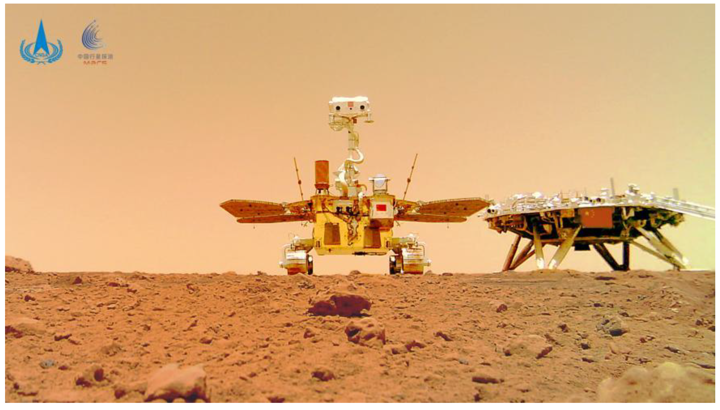
China’s Mars rover Zhurong landed on the southern region of Utopia Planitia on 15 May 2021, and it separated from the landing platform on 22 May to conduct an exploration mission on the Martian surface [1]; Figure 1 shows the image of Zhurong and its landing platform on Mars. As of 31 December 2021, Zhurong has worked on the surface of Mars for 225 Martian days and traveled a total of more than 1400 m south from its landing platform. In order to explore scientific targets, Zhurong inevitably passed through complex terrains with slip-prone areas, which called for better research on slip.

Zhurong is a six-wheel rover, which can be seen as a special kind of wheeled robot working on Mars. For a wheeled robot, slip means the actual velocity of the wheel different from the command velocity, which can be regarded as a measure of the lack of traction [2]. Slip directly leads to deviation from the scheduled path and the inability to reach targeted goals. A high slip means a severe lack of traction, which can cause wheel sinkage and even permanent immobility [3,4,5]. Most Mars and Lunar rovers had suffered slip-related hazards of varying degrees. For example, the rovers Yutu and Curiosity fortunately escaped from the high slips, and the rover Opportunity resumed movement after being entrapped for five weeks; in the worst case, the rover Spirit experienced significant slips and became stuck with permanent immobility at a stationary science platform. Therefore, it is essential to focus on slip for Zhurong’s safety.

Roughly speaking, researches on rover slip mainly focus on the following three aspects:

(1)

Model-based approach. Slip is caused by the complex interaction between the wheel and soil, which allows the estimation of the wheel-level slip by utilizing accurate kinematic and dynamical equations with a slip variable [6,7]. Some research has also focused on the enhancement of 3D kinematic models to predict the body-level slip for articulated, wheeled mobile robots [8,9,10,11]. The model-based approach explains slip from the perspective of motion and force mechanisms, but the estimation accuracy is dependent on the knowledge of soil parameters and the accuracy of the model, which is not the best choice for a planetary exploration.

(2)

Visual-based approach. Visual odometry is a reliable source of information, which is widely used in planetary explorations. Its main working principle is that in the process of movement, image data are collected from the surrounding environment through the camera, a continuous image sequence is used as the input signal, and its motion estimation is obtained by calculating its own pose change [12,13]. However, it has some limitations for planetary rovers, such as the sequence image matching calculation cost being high [14], the feature point matching on the surface features being sparse or the shadow area being limited, and it is not suitable for high-speed operation environments (>0.8 m/s), as the image would appear blurry in a high-speed motion environment [15].

(3)

Data-based approach. Based on the data mining algorithm, the collected historical data are used as the input, and the corresponding slip observations are used as the output, so as to train to obtain the corresponding slip estimation value. Angelova et al. [16,17] established a nonlinear regression mapping relationship between terrain geometry and slip by using a locally weighted projection regression (LWPR) and neural network, and the obtained models had a good slip prediction performance. The dataset used to train and validate the models was all obtained on completely natural, off-road terrains. Gonzalez et al. [2] transformed the slip value estimation problem into a classification problem through several machine learning algorithms, and they used signals of the Inertial Measurement Unit to predict the slip level (low, moderate, or high). This method was designed for the wheel-level slip, not the body-level slip. Rothrock et al. [18] presented slope slip methods, which were established based on data collected in the Jet Propulsion Laboratory Mars Yard. The models were analyzed by data from the Mars rover Curiosity, the results showing a good prediction performance in small rock and bedrock terrains, but could not fully predict the slip of the rover in sand. Cunningham et al. [19] proposed adjusting the model based on the on-orbit slip data, which significantly improved the prediction performance in sand. These researches indicated that a data-based approach provides adaptability in complex environments without the involvement of detailed mechanical models, overcoming the dependence on images of environmental characteristics. The data-based approach is becoming a common trend in slip research. So far, however, there has been little research considering the difference in environmental conditions between Earth and Mars, especially regarding the reduced gravity on Mars [20].

In this paper, the primary aim is to establish a slip estimation model for the Mars rover Zhurong, which can be used to assess the risk level of slip, as well as correct the path planning. A data-based approach is selected to establish the models, and we collected data through ground indoor tests. In order to simulate the situation of Zhurong on Mars as much as possible, the test site was equipped with a low-gravity simulation device and simulated Mars soil. Slip estimation models were built using a back propagation neural network (BP), and an optimized BP based on a genetic algorithm (GA-BP). The obtained models were applied to estimate longitudinal slip (slip_x) and lateral slip (slip_y) using on-orbit data. Then, the path planning points were corrected with the slip prediction values and compared with the actual path points, which verified the feasibility of the model.

The rest of this paper is arranged as follows: Section 2 introduces the ground tests and on-orbit validation Section 3 illustrates the training methods, Section 4 displays the training results obtained through ground tests and the estimation results compared to on-orbit real data, and Section 5 presents the conclusion.

2. Ground Tests and on-Orbit Validation

This research was designed in two parts: the ground test and on-orbit validation. The ground test was used to collect data to train the model and to verify it by using the on-orbit data. The ground testing site and on-orbit situation were described in detail as follows.

2.1. Ground Tests

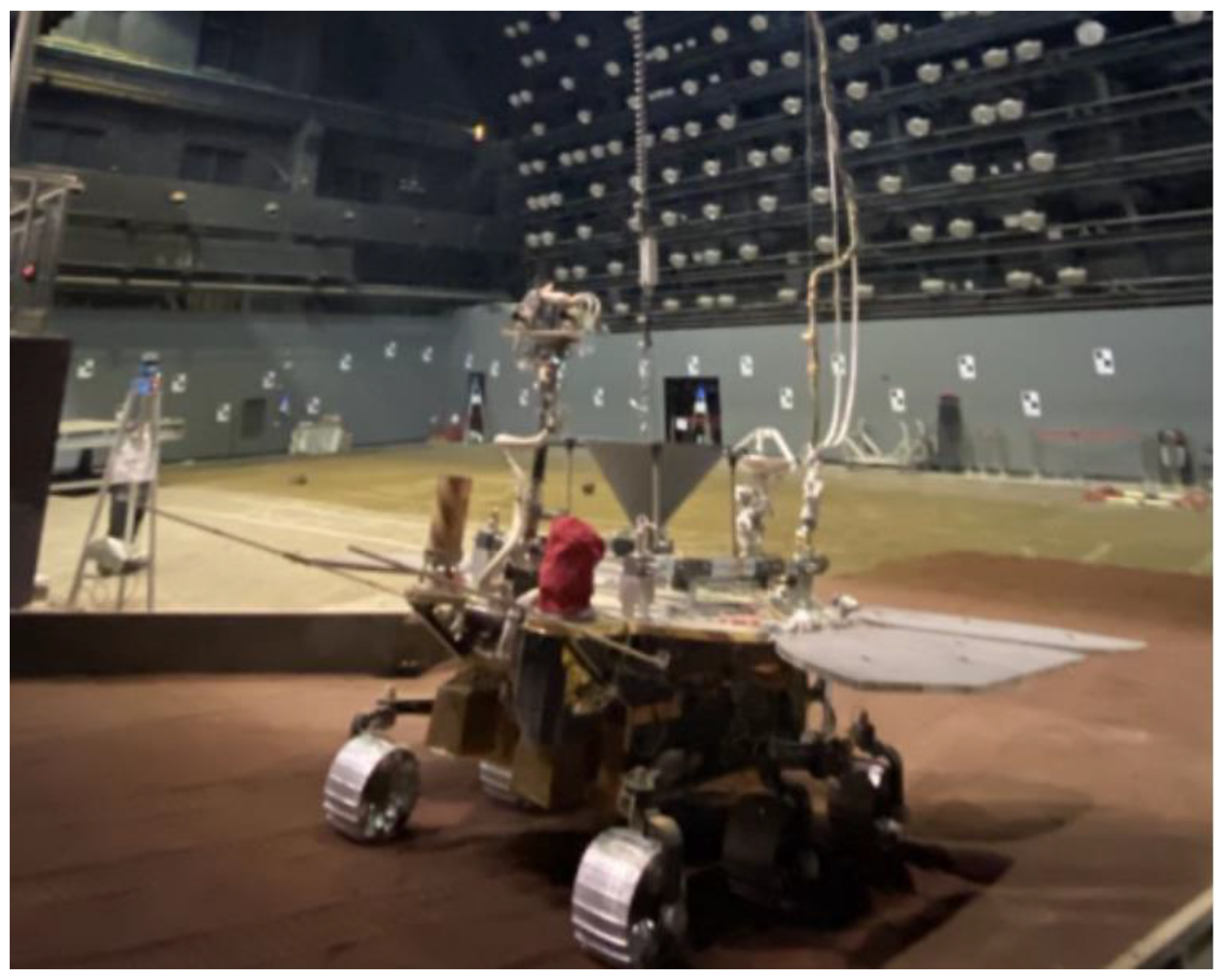
The ground tests were performed in the Chinese Academy of Space Technology. The indoor test site was composed of a horizontal area (25.3 m × 13.2 m) and an adjustable angle ramp area (8 m × 5 m), and the simulated angle could increase up to 35° [21]. Figure 2 displays the indoor test site of ground tests. To simulate the situation of Zhurong on the surface of Mars as much as possible, the test site was equipped with the following key devices or equipment.

(1)

Low-gravity simulation device. For the gravitational acceleration for Mars, which is about 40% of that on Earth, the whole test site was equipped with a low-gravity simulation device to provide a simulated Martian gravity environment for the rover, so that the vertical pressure of each wheel always stayed consistent with that on Mars. The low-gravity simulator had the ability to follow the movement of the rover and the simulation effect remained stable during tests [22].

(2)

The validator of Zhurong. The rover used in tests was the validator of Zhurong, whether regarding the structural configuration, sensor configuration, or material, it was largely the same as Zhurong.

(3)

Simulated soil. The soil is an important part of the surface environment of Mars, and the mechanical parameters of the soil are closely related to the wheel movement [23]. The simulated Mars soil, named JLU Mars-2, was used in this paper, and was laid out on the test site with a thickness of more than 500 mm [21]. The JLU Mars-2 used volcanic ash as the raw material, and the mechanical parameters of the soil were adjusted through a sprinkling and compaction process;

Table 1. The mechanical parameters of JLU Mars-2.

$k_c$($\mathrm{kPa}\cdot {\mathrm{m}}^{-(\mathrm{n}+1)}$)	$k_{\phi }$($\mathrm{kPa}\cdot {\mathrm{m}}^{-(\mathrm{n}+2)}$)	n	c (kPa)	$\phi$ (°)	k (m)
15.69	983.36	1.023	0.609	37.2	0.019

* $k_c$: the cohesive modulus of the soil; $k_{\phi }$: the frictional modulus; n: slip sinkage exponent; c: cohesion; $\phi$: internal friction angle; k: shear deformation modulus.

presents the mechanical parameters of JLU Mars-2 [24,25].

Figure 2. The indoor test site of ground tests.

Figure 2. The indoor test site of ground tests.

2.2. On-Orbit Validation

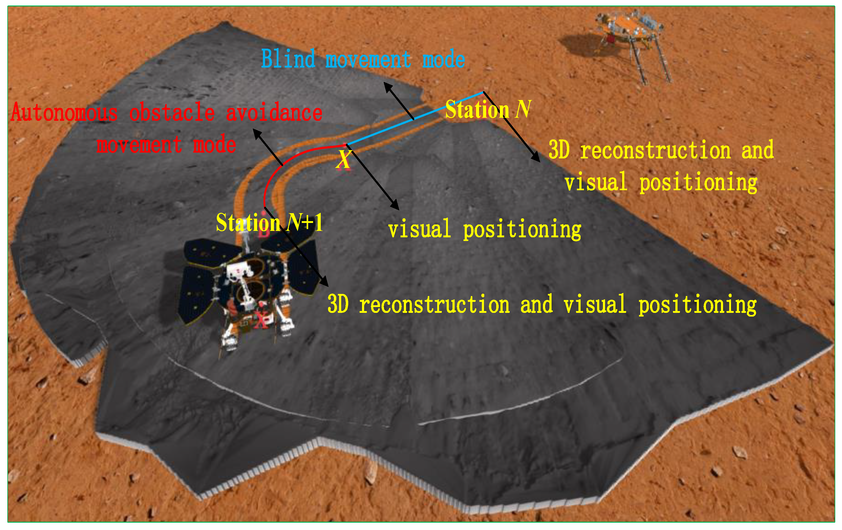
The designed life of Zhurong was 90 Mars days. Within the design life, Zhurong operated in a highly efficient detection mode, and traveled a total of 899 m with 57 movements [26,27], 15.7 m on average each time, and the longest planning distance for a single time was 26.8 m, which posed a challenge to the visual positioning accuracy of the Mars rover. To solve this problem, Zhurong would have a short stay between adjacent stations for imaging, and its imaging area overlapped with the two adjacent stations, so as to obtain precise positioning, the specific process was as follows:

(1)

Step 1: Station N. When Zhurong arrived at Station N (as shown in Figure 3), a 3D reconstruction of the environment and the visual positioning was performed. Selecting the middle point X and the target point Station N+1 based on the environment information and generating the Station N-X path planning strategy.

(2)

Step 2: Station X. Zhurong drove to the Station N-X according to the instructions, which were called the blind movement mode. It performed a visual positioning at point X to obtain the relative position of point X to Station N.

(3)

Step 3: Station N+1. Then, Zhurong drove to the X-Station N+1 section using the autonomous obstacle avoidance movement mode. When it arrived at Station N+1, step one was repeated.

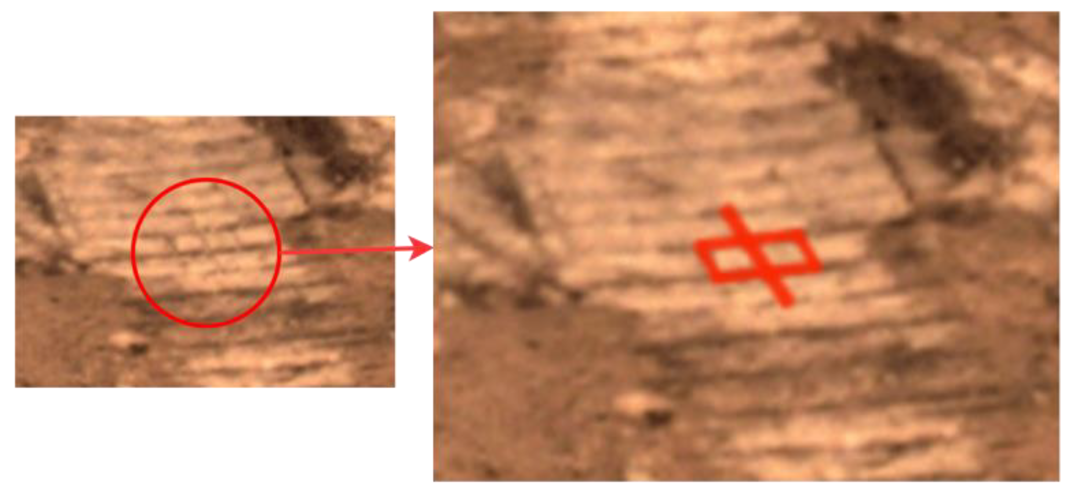
From the above described process, when Zhurong drove using blind movement mode in step two, we knew its planning path and the actual end point of arrival. It was available for the on-orbit slip validation. The wheel of the Zhurong Mars rover is printed with the Chinese word “中”. When driving on the surface of Mars, the distance and position of two adjacent words in the rut mark (as shown in Figure 4) can be used to assist in judging whether the rover has slipped.

Figure 3. The schematic diagram of Zhurong’s station.

Figure 3. The schematic diagram of Zhurong’s station.

3. Method

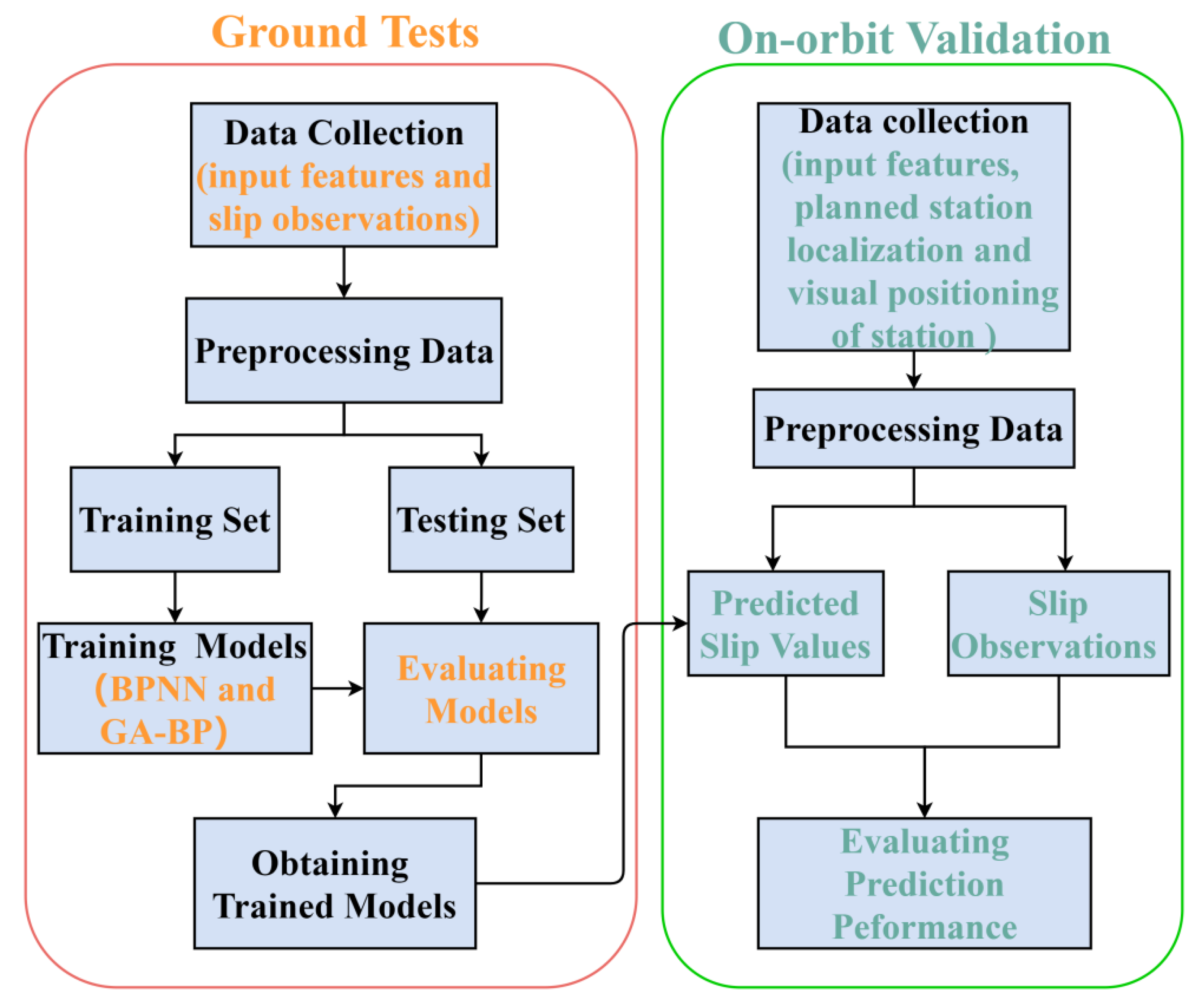
The research work of this paper is displayed in Figure 5. The ground tests were randomly divided into training set and testing set. Training of the model using machine learning algorithms on the training set and the performances of the models were evaluated on the testing set. Then, models were validated using on-orbit data. In this section, we illustrate several key issues in the model establishment and verification: the input features selection, output calculation, dataset division, training method, and evaluation method.

3.1. Input Features Selection

The goal of input features selection was to select the relevant features from available sensor inputs for good model accuracy [28]. In this work, four features were chosen to form input feature vector to the algorithms: (1) the rover’s pitch; (2) the rover’s roll; (3) the average current I of six-wheel driving motors; (4) the average angular velocity w of six-wheel driving motors.

(1), (2), and (3) were used for slip prediction in previous work [16,17,29,30]. The rover’s pitch and roll corresponded to the terrain geometry [16], and directly reflected the vertical loads acting on wheels. Additionally, there was a linear relationship between driving motor current and torques applied to the wheels. According to the complex relation between force and the wheel–soil interface, changes in vertical load and driving torque would affect wheel slip, so (1), (2), (3), and slip could be related [30]. There was some correspondence between wheel angular velocity and slip because of non-ideal motor behaviors [31]; it was useful to select (4) as one of the input features.

3.2. Output Calculation

Slip s means the actual velocity of the was wheel different from the command velocity for each of the wheels; it is defined as Equation (1).

$$s=(v_c-v)/v_c$$

(1)

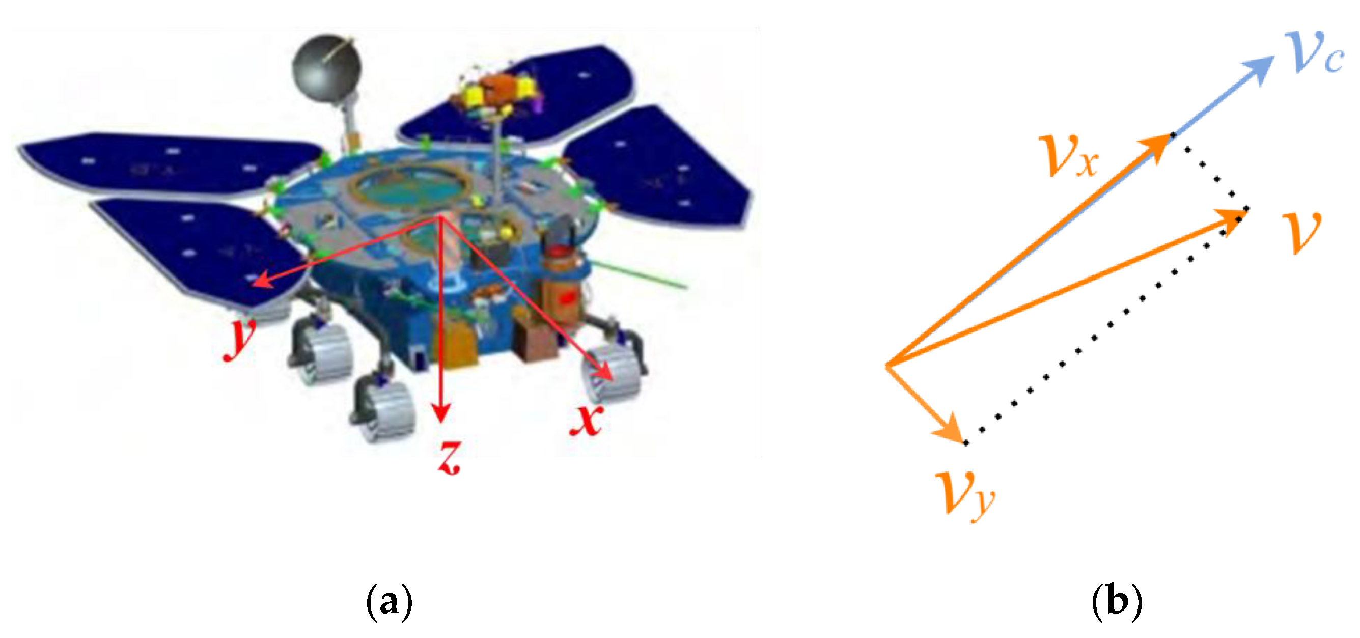
where v and v_c are the actual velocity and the expected velocity of the wheel, respectively. Similar to the wheel slip, calculating the rover slip needed both the expected velocity of the rover and the actual velocity of the rover. Slip was measured in the rover body frame as shown in Figure 6a, and included longitudinal slip (slip_x), lateral slip (slip_y), and rotational slip (slip_z) [29]. This paper reports on slip_x and slip_y of the rover, which are defined as Equations (2) and (3), respectively [32].

$$\mathrm{slip}\_x=(v_c-v_x)/v_c$$

(2)

$$\mathrm{slip}\_y=v_y/v_c$$

(3)

where $v_c$ is the command velocity of rover, $v_x$ is the actual longitudinal velocity, and $v_y$ is the lateral slip velocity of the rover (Figure 6b).

3.3. Dataset

The raw data collected in ground tests and their usage are summarized in

Table 2. The data collected in ground tests.

Raw Data	Sampling Frequency	Usage
The rover’s pitch	20 Hz	Input feature (1)
The rover’s roll	20 Hz	Input feature (2)
The current of each wheel’s driving motor	1 Hz	Calculate the input feature (3)
the angular velocity of each wheel’s driving motor	1 Hz	Calculate the input feature (4)
The position of rover	20 Hz	Calculate the slip of rover

. The position and attitude of the rover were measured by the global indoor positioning system (iGPS) with sampling frequency of 20 Hz, while the sampling frequency of current and angular velocity was 1 Hz. We set the step time of the analysis as 0.05 s, and the current and angular velocity had to be interpolated. In order to ensure the rationality and accuracy of the interpolation, data segments with large angular velocity or current fluctuations were not selected.

The hold-out method was used to randomly split the ground tests data into the training set (66.7%) and testing set (33.3%). After that, the data were normalized.

3.4. Learning Algorithms

In this paper, BP neural network was used to train models for their good nonlinear mapping ability and self-adaptability, as well as strong robustness and fault tolerance [33,34]. The simple learning rules were easy to implement [35]. However, the models were prone to trap in local optima. In order to achieve better performance of models, GA was used to optimize the initialization weights and thresholds of the BP, based on the global search ability of GA. In our previous work, we used BP and GA-BP to establish slip_x models [36]. In this paper, we aimed to establish slip models which could predict slip_x and slip_y at the same time, so that the models could not only be used for slip early warning, but also guide path planning.

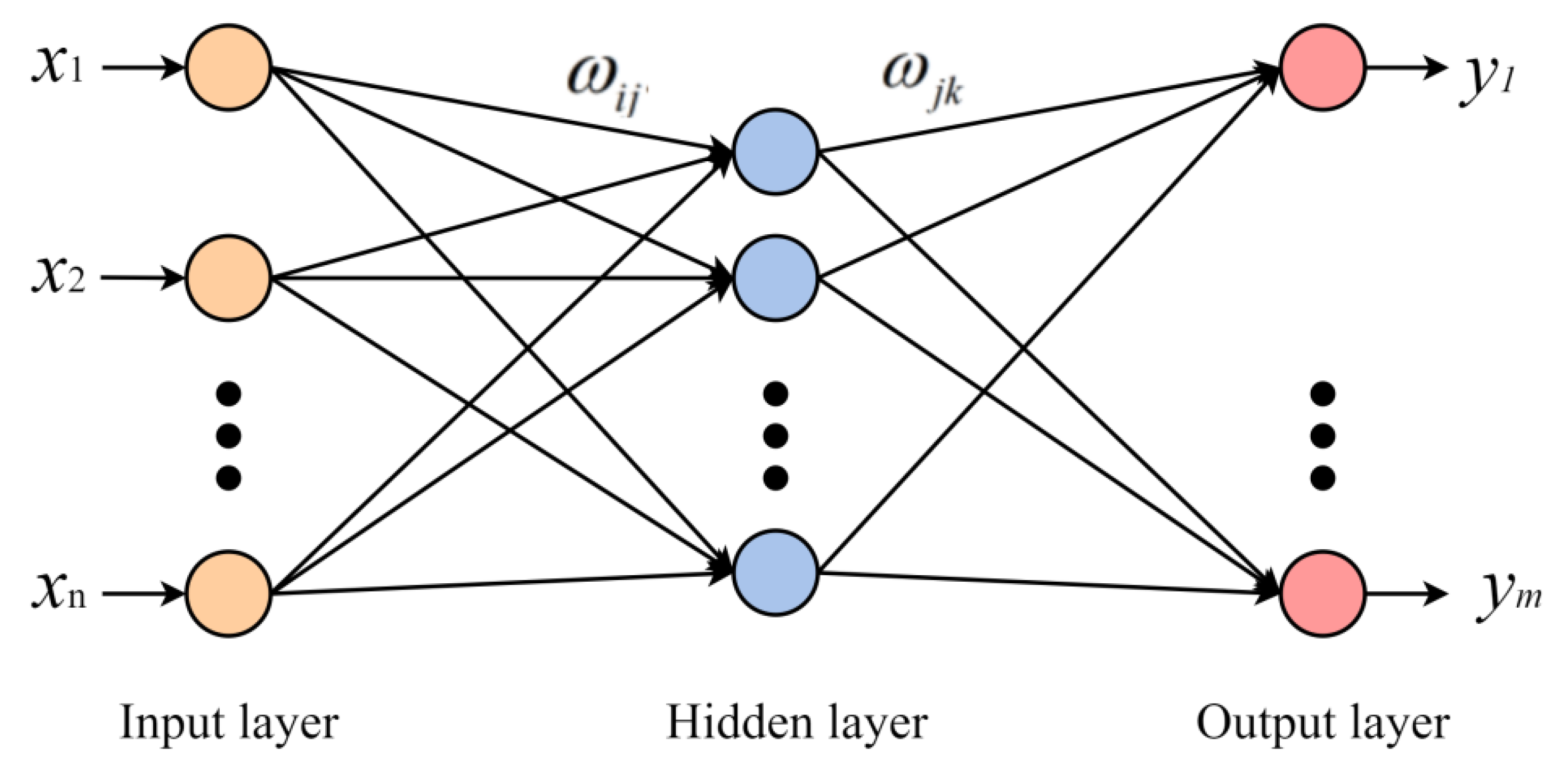
BP neural network presented a multi-layer structure, as shown in Figure 7. It is typically composed of three layers: input layer, hidden layer, and output layer [37].

Input signals (x₁,x₂,…,x_n) were received by the input layer and reached the output layer after being processed by the hidden layer. Neurons in adjacent layers were connected by different weights (${\omega }_{ij}$,${\omega }_{jk}$).

$$h_j=f\left|{\displaystyle \sum {\omega }_{ij}{x}_i-a_j}\right|,j=1,2,\dots ,l$$

(4)

$$O_k=\psi \left|{\displaystyle \sum h_j}{\omega }_{jk}-b_k\right|,k=1,2,\dots ,m$$

(5)

where h_j and $O_k$ are the output of the hidden layer and output layer, respectively. ${\omega }_{ij}$ is the weight from the i_th input layer neuron to the j_th hidden layer neuron, and ${\omega }_{jk}$ is the weight from the j_th hidden layer neuron to k_th output layer neuron. The hidden layer threshold is a_j and the output layer threshold is b_k. f (x) and $\psi (h)$ are the active function of the hidden layer and output layer, f (x) is the sigmoid type of nonlinear function, and $\psi (h)$ is the linear function.

When the actual output (y₁,y₂,…,y_m) could not obtain the expected output values, it switched to error back propagation, and the connection weights and thresholds were modified according to the error, so that the output values would constantly approach the expected output.

GA is a self-adaptive global optimization algorithm by simulating the genetic and evolution process of living beings in the natural environment. It encodes the parameters of certain problems as chromosomes, performing the selection based on survival of the fittest, and then obtaining new generations of individuals through crossover and mutation operation [38].

In this paper, GA was used to optimize the initial connection weights and thresholds of BPNN. The optimization process was described as follows.

(1)

Step 1: Encoding

When the topology of BP was determined, connection weights and thresholds were encoded into chromosomes. The encoding length L was defined as follows:

$$L=m+n+ml+ln,$$

(6)

where m, l, and n are the numbers of neurons in input layer, hidden layer, and output layer, respectively.

(2)

Step 2: Calculating fitness function

In order to obtain better performance of model, we defined the fitness function $f_{fit}$ as Equation (7).

$$f_{fit}=1/({\eta }_1\cdot {\displaystyle \sum {({\widehat{s}}_{xi}-s_{xi})}^2}+{\eta }_2\cdot {\displaystyle \sum {({\widehat{s}}_{yi}-s_{yi})}^2})$$

(7)

where ${\widehat{s}}_{xi}$ and ${\widehat{s}}_{yi}$ represent the predicted slip_x and slip_y, respectively. $s_{xi}$ and $s_{yi}$ are the actual slip_x and slip_y, respectively. ${\eta }_1$ and ${\eta }_2$ represent coefficients.

(3)

Step 3: Genetic operations

Genetic operations included three basic genetic operators: selection, crossover, and mutation.

Selection was to select superior individuals from the population and eliminate inferior individuals based on fitness values. For a population of size N, where the fitness of individual i was $f_{fit\_i}$, the probability of i being selected was $p_i$:

$$p_i=f_{fit\_i}/{\displaystyle \sum f_{fit\_j}}$$

(8)

The crossover was to recombine part of the structure of the selected parent individuals to generate new individuals. The crossover operator adopted the single-point crossover operator, an intersection was randomly selected, and two parent individuals swapped at the front or back of the point to produce new individuals.

The new individuals formed after the crossover operation had a certain probability of mutation. Similar to the selection operation, this operation was based on probability. Generally speaking, the mutation probability was set very small.

(4)

Step 4: Iterative optimization

When termination condition was met, the optimization process stopped, and the obtained optimized weights and thresholds were assigned to the BPNN.

BPNN used the optimized result weights and thresholds to perform training, and could avoid the prediction results from falling into the local optimal solution.

3.5. Evaluation of Models

In this paper, mean absolute error (MAE) and root mean square error (RMSE) were used to evaluate the accuracy of the slip model.

$$\mathrm{MAE}\_x=\frac{1}{n}{\displaystyle \sum _{i=1}^n\left|{\widehat{s}}_{xi}-s_{xi}\right|}$$

(9)

$$\mathrm{MAE}\_y=\frac{1}{n}{\displaystyle \sum _{i=1}^n\left|{\widehat{s}}_{yi}-s_{yi}\right|}$$

(10)

$$\mathrm{RMSE}\_x=\sqrt{{\displaystyle \sum _{i=1}^n\frac{{({\widehat{s}}_{xi}-s_{xi})}^2}{n}}}$$

(11)

$$\mathrm{RMSE}\_y=\sqrt{{\displaystyle \sum _{i=1}^n\frac{{({\widehat{s}}_{yi}-s_{yi})}^2}{n}}}$$

(12)

4. Results and Discussion

4.1. Ground Tests

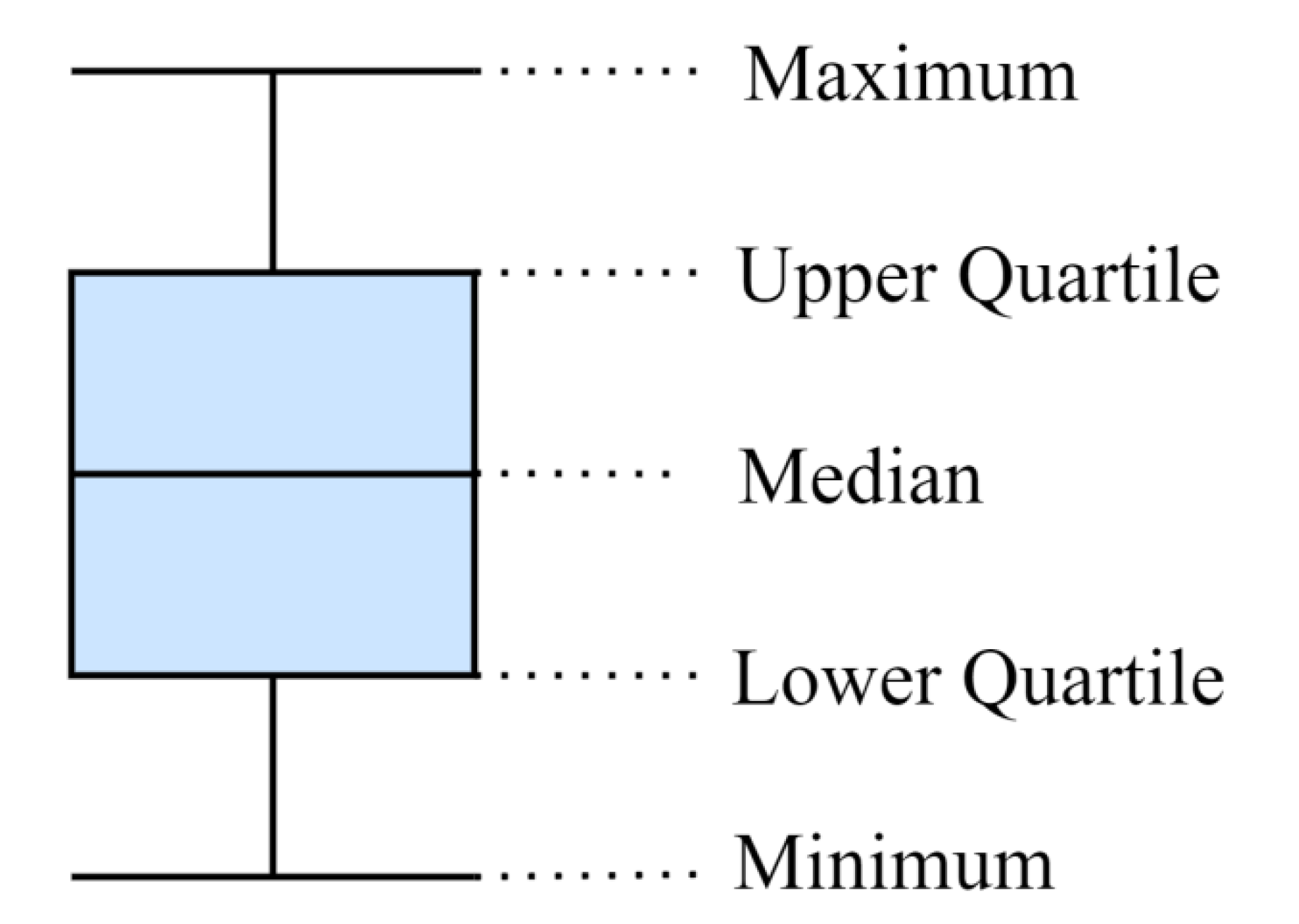
We repeated the hold-out validation on the models of each type ten times to ensure a better stability and reliability of results. Twenty models were obtained in total with BP and GA-BP; the prediction results are summarized in detail in

Table 3. Prediction results of BP and GA-BP.

BP					GA-BP
Group Number	Slip_x		Slip_y		Group Number	Slip_x		Slip_y
	MAE	RMSE	MAE	RMSE		MAE	RMSE	MAE	RMSE
(1)	3.314	4.300	1.239	1.652	(1)	3.163	4.022	1.150	1.577
(2)	3.058	4.114	1.137	1.511	(2)	3.082	4.045	1.184	1.523
(3)	3.165	4.156	1.215	1.621	(3)	3.138	4.091	1.127	1.487
(4)	3.123	4.112	1.263	1.618	(4)	3.063	4.059	1.190	1.537
(5)	3.147	4.140	1.161	1.539	(5)	3.121	4.061	1.117	1.450
(6)	3.020	4.035	1.233	1.595	(6)	2.987	3.961	1.131	1.474
(7)	3.224	4.228	1.118	1.485	(7)	3.186	4.096	1.058	1.414
(8)	3.275	4.277	1.244	1.637	(8)	3.148	4.144	1.194	1.529
(9)	3.149	4.195	1.129	1.499	(9)	3.175	4.094	1.115	1.470
(10)	3.170	4.169	1.093	1.476	(10)	3.021	4.001	1.131	1.522
Mean	3.164	4.173	1.183	1.563	Mean	3.108	4.058	1.140	1.498

. A boxplot was used to show the distribution of evaluation results for each model in the following, as shown in Figure 8: the maximum value, upper quartile, median, lower quartile, and minimum value are represented from top to bottom.

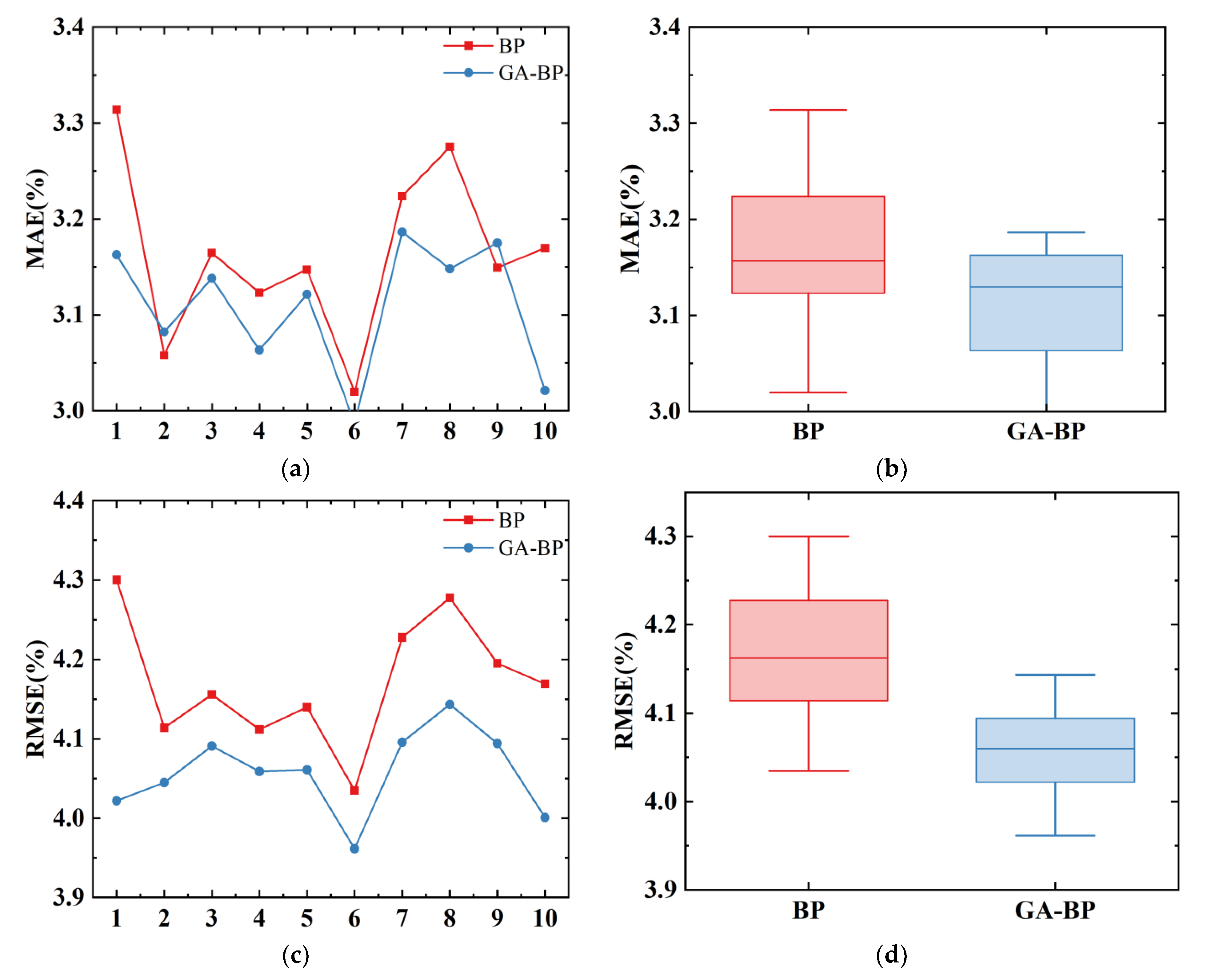
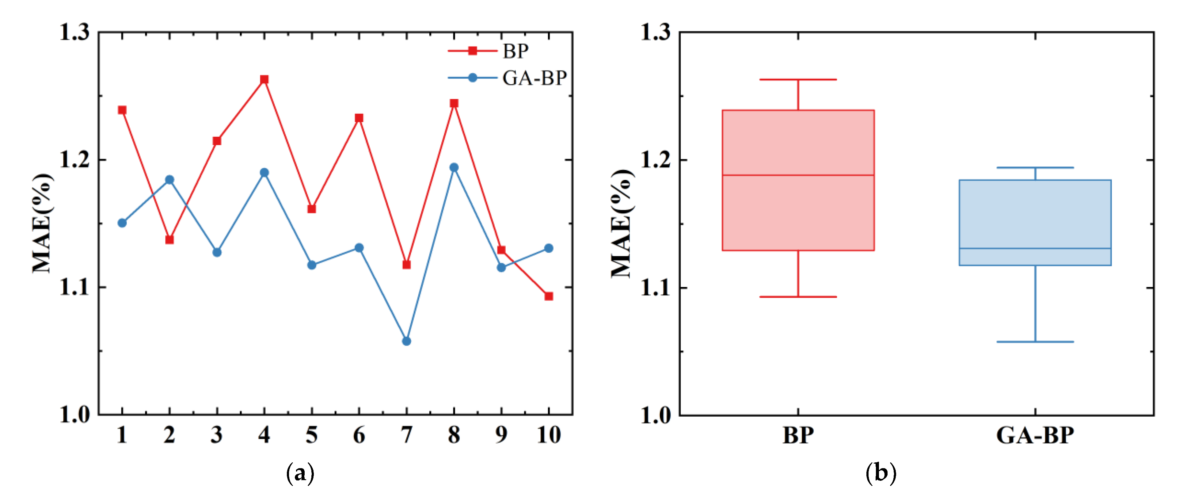
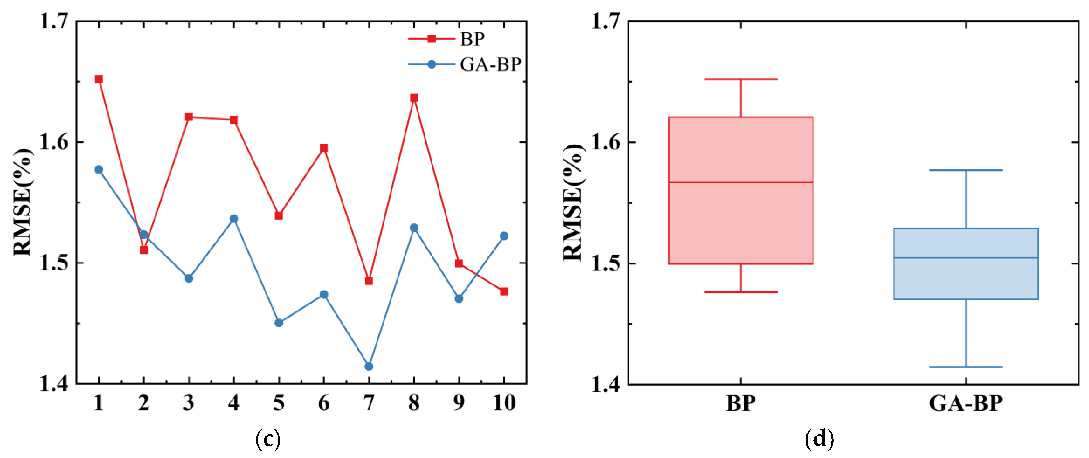
Figure 9 and Figure 10 present the prediction results of five test groups for slip_x and slip_y, respectively. As can be seen in Figure 8a,c and Figure 9a,c for most test groups, after GA optimization, the MAE and RMSE of slip_x and slip_y were reduced to varying degrees at the same time. Combining the data in Table 2 to obtain the MAE results for slip_x as an example, the MAE results of BP were between around 3.020 and 3.314%, with an average of 3.164%, and the MAE results of GA-BP were between around 2.987 and 3.216%, with an average of 3.108%. The MAE predicted by GA-BP was decreased by 0.056% on average compared to the MAE predicted by BP. It can be seen that the GA-BP model had a higher prediction accuracy for slip_x and slip_y. From Figure 8b,d and Figure 9b,d, the GA-BP prediction was more concentrated and the model performance was more stable.

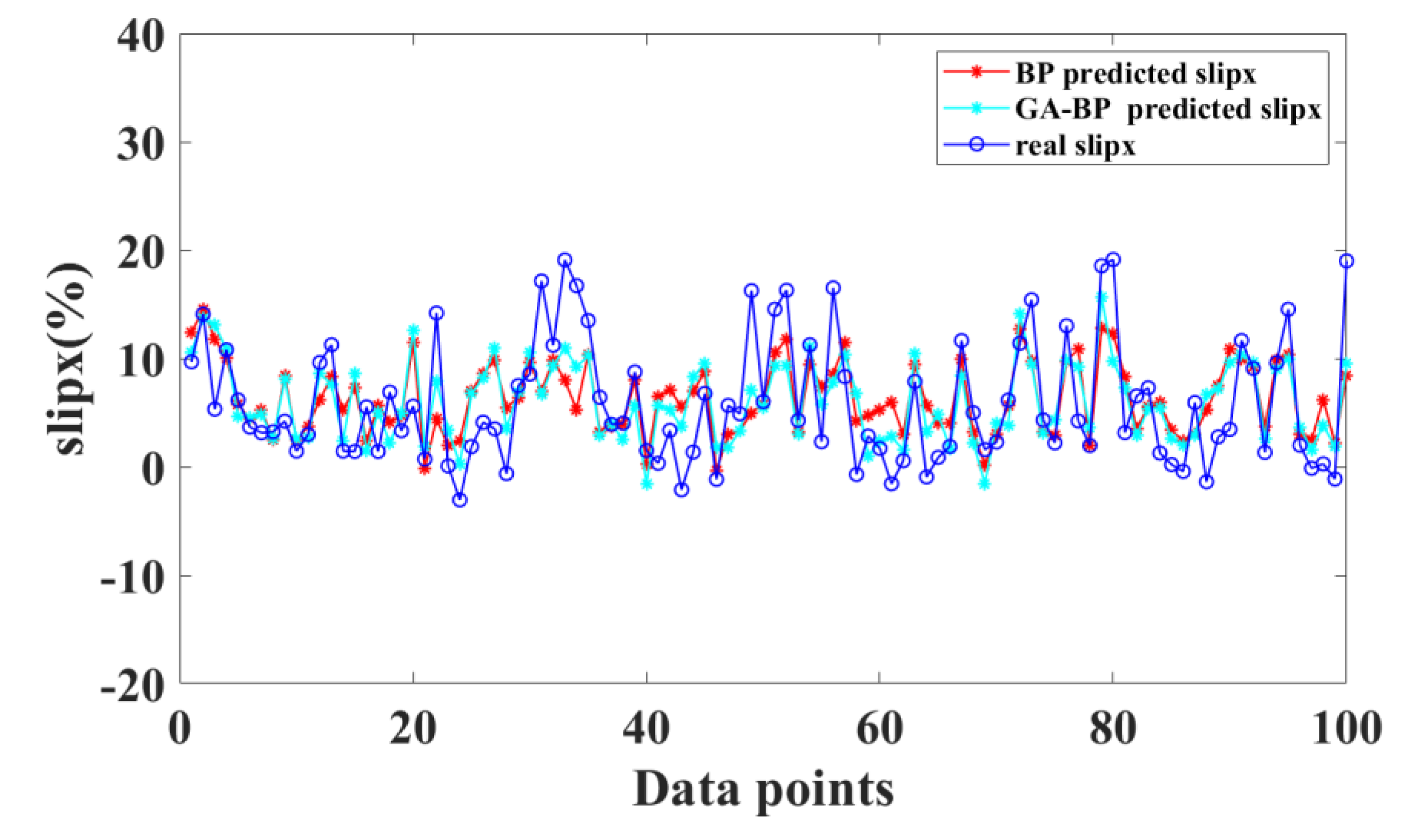
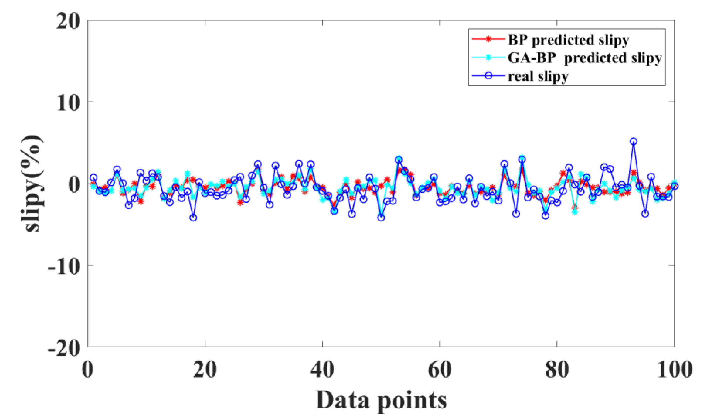
Figure 11 and Figure 12 show part of the prediction results of slip_x and slip_y in group (1), respectively. Since the testing set data were randomly selected, the testing data points were not continuous, and so it was not suitable to show all testing data since they were too dense and no trend could be seen. In order to show the prediction results more clearly, Figure 11 and Figure 12 only show the prediction of 100 data points. The predicted results were consistent with the trends of actual values, but the actual slip_x and slip_y had a larger variation range, while the prediction data of BP and GA-BP were relatively concentrated. According to statistics, out of 1911 test points in group (1), there were 987 slip_x points predicted by GA-BP, which was closer to the actual slip_x than the points predicted by BP, and the amount of 1078 slip_y GA-BP prediction points was closer to the actual slip_y than the BP prediction points. It can be seen from the above analysis that GA-BP had a higher prediction accuracy than BP.

4.2. On-Orbit Validation

The BP models and GA-BP models which learned from the ground tests data were validated using Zhurong’s on-orbit data. The real-time actual coordinates during Zhurong’s walking process could not be obtained, so it was impossible to directly verify the accuracy of the predicted slip values during the walking process. We could convert the predicted slip_x and slip_y into a longitudinal offset ∆x and lateral offset ∆y, respectively. Therefore, we could obtain the slip prediction corrected path points. When we compared the end point of the predicted path with the actual points, the predictive effect of the models could be seen. The specific implementation steps were as follows:

(1)

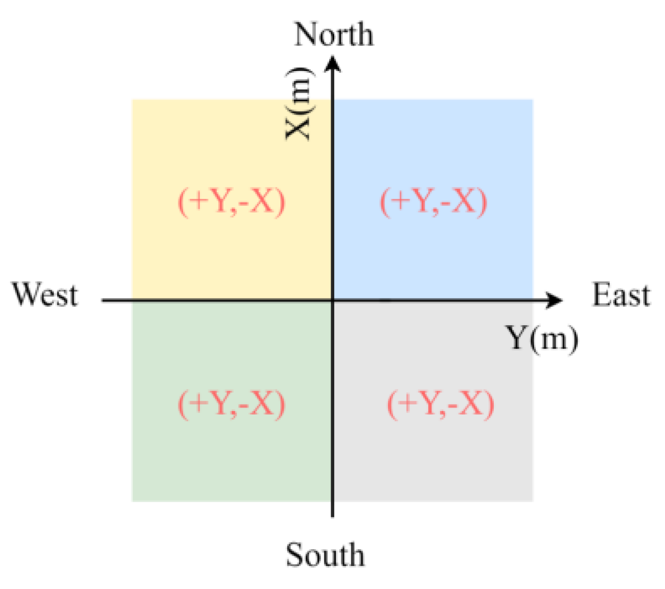
The planning path could be drawn from the planning curvature, planning distance, and planning target point. Positive curvatures represented right turns, negative curvatures represented left turns, and a larger planning curvature value meant a smaller steering radius. According to the introduction in Section 2.2, Zhurong travelled according to the planning path during the blind walking stage. Figure 13 shows the coordinates of the planning path. Each starting point was regarded as (0,0), with +Y facing east and +X facing north. We could draw the planning path based on the planning curvature, planning target point, and planning distance.

(2)

Visual positioning was performed when Zhurong completed a blind walk to obtain the real positioning of the actual point.

(3)

The offsets ∆x and ∆y of path points were calculate from the predicted slip, and so we could obtain a serial of predicted path points with slip correction. These predicted path points formed a predicted path. It should be noted that the ∆x and ∆y of slip prediction were based on the rover’s body coordinate system, and need to be transformed into ∆X and ∆Y through a coordinate transformation.

(4)

We compared the coordinates of the end point of the BP and GA-BP predicted path with the actual point.

Figure 13. Path planning coordinates.

Figure 13. Path planning coordinates.

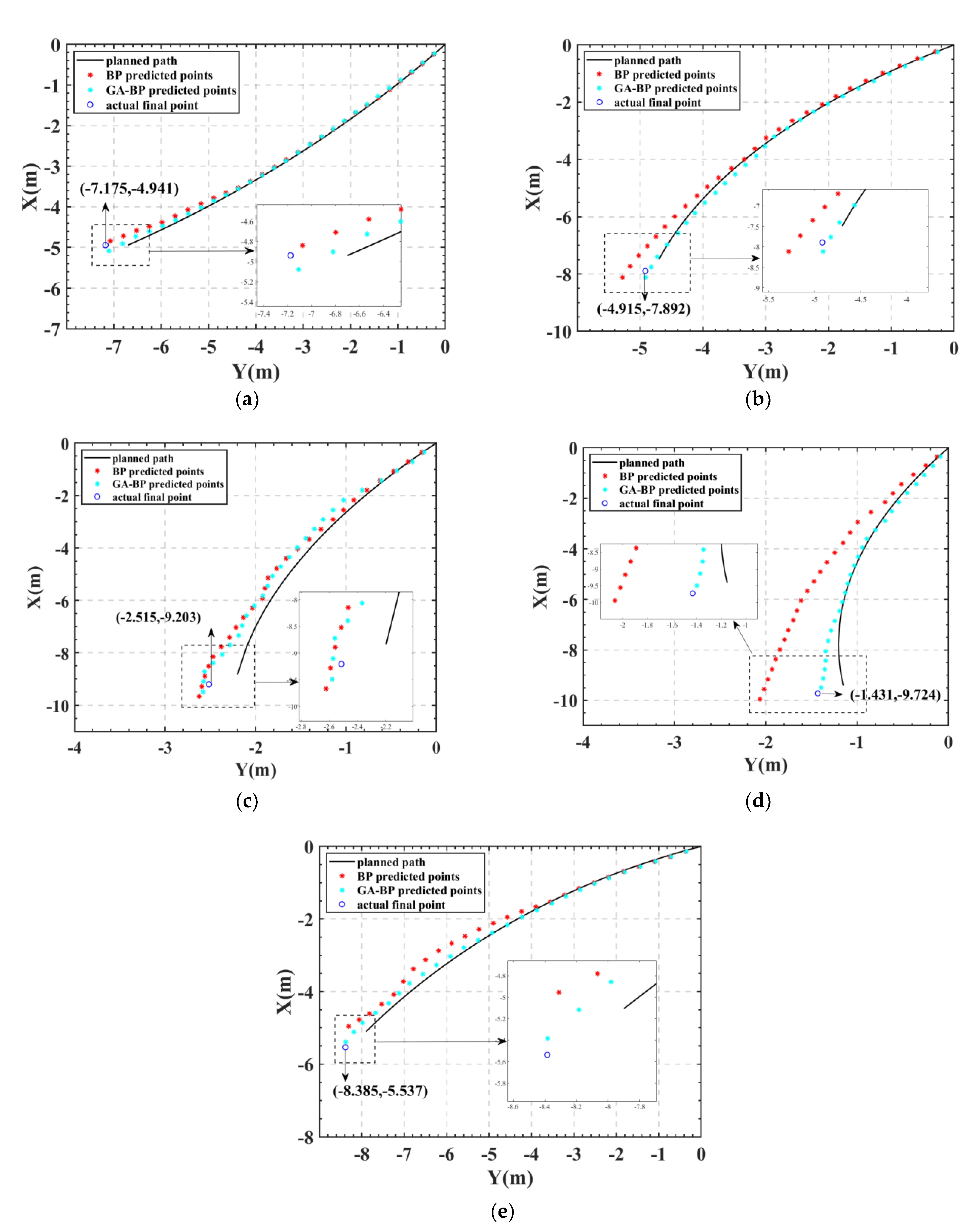
In this paper, an on-orbit validation was conducted based on data obtained from mid-June 2021 (sol.27–sol.36) with five movements.

Table 4. Planning end points and actual end points of arrival.

Sol	Planning Curvature (1/m)	Planning Distance (m)	Planning Points		Actual Points		Deviation
			X_Plan (m)	Y_Plan (m)	X_Actual (m)	Y_Actual (m)	∆X (m)	∆Y (m)	∆L (m)
27	0.038	8.459	−4.9805	−6.7917	−4.9408	−7.1753	0.0397	−0.3836	0.3856
28	−0.071	9.196	−7.6869	−4.7449	−7.8924	−4.9153	−0.2055	−0.1704	0.2670
29	−0.037	9.635	−9.3236	−2.2155	−9.2034	−2.5153	0.1202	−0.2998	0.3230
34	−0.039	9.23	−9.107	−1.1502	−9.7244	−1.4313	−0.6174	−0.2811	0.6784
36	−0.0594	9.644	−5.1775	−7.9800	−5.5369	−8.3848	−0.3594	−0.4048	0.5413

* ∆X = (X_actual) − (X_plan); ∆Y = (Y_actual) − (Y_plan); ∆l = $\sqrt{\Delta X^2+\Delta Y^2}$.

shows the planning path information and actual end points of arrival. We could see that there was always a deviation ∆L between the actual path end point and the planning point, The maximum ∆L could be obtained as 0.6784 m.

Table 5. BP and GA-BP predicted end points of path.

Sol	BP Predicted Points		GA-BP Predicted Points		Deviation
	X_BP (m)	Y_BP (m)	X_GABP (m)	Y_GABP (m)	∆X_BP (m)	∆X_GABP (m)	∆Y_BP (m)	∆Y_GABP (m)	∆L_BP (m)	∆L_GABP (m)
27	−4.8409	−7.0760	−5.0808	−7.1068	−0.14	0.0993	0.0685	0.14085631	0.1559	−0.14
28	−8.1185	−5.2808	−8.1139	−4.90956	−0.2215	−0.3655	0.00574	0.429780712	0.2216	−0.2215
29	−9.6685	−2.6229	−9.4854	−2.5799	−0.282	−0.1076	−0.0646	0.4773843	0.2893	−0.282
34	−9.9452	−2.0637	−9.4868	−1.3970	0.2376	−0.6324	0.0343	0.669837592	0.2401	0.2376
36	−4.9544	−8.3107	−5.3848	−8.3828	0.1521	0.0741	0.002	0.587194227	0.1521	0.1521

* ∆x_GABP = (x_GABP) − (x_actual); ∆y_GABP = (y_GABP) − (y_actual); ∆l_GABP=$\sqrt{{(\Delta x\_\mathrm{GA}BP)}^2+{(\Delta y\_\mathrm{GA}BP)}^2}$.

displays the information of the BP and GA-BP predicted end points of the path. In each set of data, the ∆L_BP and ∆L_GABP were always smaller than ∆L; combined with the predicted path and planning path shown in Figure 14, we could see that the predicted end points were closer to the actual points. From the relative positional relationship between the actual end point and the planned path, it could be seen that the rover deviated to the right during the driving process. Both BP and GA-BP predicted paths simulated this movement trend, but the BP model predicted the path to a greater degree of deviation compared to the GA-BP model, which led to the BP predicting end points relatively far from the actual end point, especially in Figure 14d. The GA-BP model had a more stable prediction performance, and the GA-BP predicted paths were reasonably acceptable for showing the slip behavior of the rover during motion.

.

5. Conclusions

This paper established slip estimation models based on ground tests data, and the testing site restored the situation of the rover Zhurong on Mars from the aspects of gravity, soil, etc. Proprioceptive sensor signals were selected as the input features to train the models, which ensured models could be used in shadowed or near-featureless areas. By validating the models of Zhurong’s on-bit data, the results showed that the slip estimation models were reasonably accurate in showing the slip behavior of the rover during motion, and the proposed models had a high potential in guiding the path planning and monitoring the slip for Zhurong.

References

- Tian, H.; Zhang, T.; Jia, Y.; Peng, S.; Yan, C. Zhurong: Features and mission of China’s first Mars rover. Innovation 2021, 2, 100121. [Google Scholar] [CrossRef]
- Gonzalez, R.; Apostolopoulos, D.; Iagnemma, K. Slippage and immobilization detection for planetary exploration rovers via machine learning and proprioceptive sensing. J. Field Robot. 2018, 35, 231–247. [Google Scholar] [CrossRef]
- Gonzalez, R.; Iagnemma, K. Slippage estimation and compensation for planetary exploration rovers. State of the art and future challenges. J. Field Robot. 2018, 35, 564–577. [Google Scholar] [CrossRef]
- Gonzalez, R.; Fiacchini, M.; Iagnemma, K. Slippage prediction for off-road mobile robots via machine learning regression and proprioceptive sensing. Robot. Auton. Syst. 2018, 105, 85–93. [Google Scholar] [CrossRef] [Green Version]
- Gonzalez, R.; Chandler, S.; Apostolopoulos, D. Characterization of machine learning algorithms for slippage estimation in planetary exploration rovers. J. Terramechanics 2019, 82, 23–34. [Google Scholar] [CrossRef]
- Balakrishna, R.; Ghosal, A. Modeling of slip for wheeled mobile robots. IEEE Trans. Robot. Autom. 1995, 11, 126–132. [Google Scholar] [CrossRef]
- Liang, D.; Zongquan, D.; Haibo, G.; Jianguo, T.; Iagnemma, K.D.; Guangjun, L. Interaction mechanics model for rigid driving wheels of planetary rovers moving on sandy terrain with consideration of multiple physical effects. J. Field Robot. 2015, 32, 827–859. [Google Scholar]
- Balaram, J. Kinematic observers for articulated rovers. In Proceedings of the 2000 IEEE International Conference on Robotics and Automation, San Francisco, CA, USA, 24–28 April 2000. [Google Scholar]
- Seegmiller, N.; Kelly, A. Enhanced 3D Kinematic Modeling of Wheeled Mobile Robots. In Proceedings of the 2014 International Conference on Robotics: Science and Systems X, Berkeley, CA, USA, 23–30 January 2014. [Google Scholar]
- Seegmiller, N.; Rogers-Marcovitz, F.; Miller, G.A.; Kelly, A. Vehicle model identification by integrated prediction error minimization. Int J. Robot. Res. 2013, 32, 912–931. [Google Scholar] [CrossRef]
- Bussmann, K.; Meyer, L.; Steidle, F.; Wedler, A. Slip Modeling and Estimation for a Planetary Exploration Rover: Experimental Results from Mt. Etna. In Proceedings of the International Conference on Intelligent Robots and Systems, Madrid, Spain, 1–5 October 2018. [Google Scholar]
- Nister, D.; Naroditsky, O.; Bergen, J. Visual odometry. In Proceedings of the 2004 IEEE Computer Society Conference on Computer Vision and Pattern Recognition, Princeton, NJ, USA, 27 June–2 July 2004. [Google Scholar]
- Kilic, C.; Ohi, N.; Yu, G.; Jason, N.G. Slip-Based Autonomous ZUPT through Gaussian Process to Improve Planetary Rover Localization. IEEE Robot. Autom. Lett. 2021, 6, 4782–4789. [Google Scholar] [CrossRef]
- Maimone, M.; Cheng, Y.; Matthies, L. Two years of Visual Odometry on the Mars Exploration Rovers. J. Field Robot. 2007, 24, 169–186. [Google Scholar] [CrossRef] [Green Version]
- Gonzalez, R.; Rodriguez, F.; Guzmn, J.L.; Siegwart, R. Combined visual odometry and visual compass for off-road mobile robots localization. Robotica 2012, 30, 865–878. [Google Scholar] [CrossRef] [Green Version]
- Angelova, A.; Matthies, L.; Helmick, D.M.; Pietro, P. Learning and prediction of slip from visual information. J. Field Robot. 2010, 24, 205–231. [Google Scholar] [CrossRef]
- Angelova, A.; Matthies, L.; Helmick, D.M.; Pietro, P. Learning to Predict Slip for Ground Robots. In Proceedings of the IEEE International Conference on Robotics and Automation, Orlando, FL, USA, 15–19 May 2006. [Google Scholar]
- Brandon, R.; Jeremie, P.; Ryan, K.; Masahiro, O.; Matt, H. SPOC: Deep Learning-based Terrain Classification for Mars Rover Missions. In Proceedings of the 2016 AIAA SPACE Conferences and Exposition, Long Beach, CA, USA, 13–16 September 2016. [Google Scholar]
- Chris, C.; Masahiro, O.; Issa, N.; Jeng, Y.; William, L.W. Locally-Adaptive Slip Prediction for Planetary Rovers Using Gaussian Processes. In Proceedings of the 2017 IEEE International Conference on Robotics and Automation, Singapore, 29 May–3 June 2017. [Google Scholar]
- Parna, N.; Adriana, D.; Krzysztof, S. The effects of reduced-gravity on planetary rover mobility. Int. J. Robot. Res. 2020, 39, 797–811. [Google Scholar]
- Jia, Y.; Zhang, T.; Tian, H.; Ji, L. Experimental verification of Zhurong Mars rover. Exp. Technol. Manag. 2021, 38, 001–005. [Google Scholar]
- Sun, Z.; Zhang, H.; Jia, Y.; Wu, X.; Shen, Z.; Ren, D.; Dang, Z.; Wang, C.; Gu, Z.; Chen, B. Ground validation technologies for Chang’E-3 lunar spacecraft. Sci. Sin. Technol. 2014, 44, 368–376. [Google Scholar]
- Dang, Z.; Chen, B. Analysis on Physical and Mechanical Properties of Martian Soil. J. Deep Space Explor. 2016, 3, 129–144. [Google Scholar]
- Xue, L. Engineering of Martian Soil Simulant and in Site Identification of Terrain Parameter for Planetary Rovers. Ph.D. Thesis, Jilin University, Changchun, China, 2017. [Google Scholar]
- Gai, H. Estimation Research of Mechanical Parameters of Planet Soil Based on Wheel-Soil Model. Master’s Thesis, Jilin University, Changchun, China, 2019. [Google Scholar]
- China’s Mars Rover Zhurong Complete Its Predetermined Mission(1/3). Available online: http://www.ecns.cn/hd/2021-08-18/detail-ihaqcyws4450242.shtml (accessed on 20 October 2021).
- Chen, B. Mars Exploration technology. Sci. China—Technol. Sci. 2022; accepted. [Google Scholar]
- Isra, A.T.; Najwa, A. A Convolutional Neural Network for Improved Anomaly-Based Network Intrusion Detection. Big Data 2020, 9, 233–252. [Google Scholar]
- Ma, H.; Yang, H.; Li, Q.; Liu, S. A geometry-based slip prediction model for planetary rovers. Comput. Electr. Eng. 2020, 86, 106749. [Google Scholar] [CrossRef]
- Lauro, O.; Daniel, C.; Giulio, R.; Johann, B. Current-Based Slippage detection and odometry correction for mobile robots and planetary rovers. IEEE Trans. Robot. 2006, 22, 366–378. [Google Scholar]
- Kruger, J.; Rogg, A.; Gonzalez, R. Estimating wheel slip of a planetary exploration rover via unsupervised machine learning. In Proceedings of the 2019 IEEE Aerospace Conference, Big Sky, MT, USA, 2–9 March 2019. [Google Scholar]
- Hiroaki, I.; Takashi, K.; David, W. Robust Path Planning for Slope Traversing Under Uncertainty in Slip Prediction. IEEE Robot. Autom. Lett. 2020, 5, 3390–3397. [Google Scholar]
- Yu, J.; Su, Y.; Liao, Y. The Path Planning of Mobile Robot by Neural Networks and Hierarchical Reinforcement Learning. Front. Neurorobotics 2020, 14, 1–12. [Google Scholar] [CrossRef]
- Lei, F.; Zhu, S.; Lin, F.; Su, Z.; Zhang, C. Detection of Oil Chestnuts Infected by Blue Mold Using Near-Infrared Hyperspectral Imaging Combined with Artificial Neural Networks. Sensors 2018, 18, 1944. [Google Scholar]
- Zou, M.; Xue, L.; Gai, H.; Dang, Z.; Wang, S.; Xu, P. Identification of the shear parameters for lunar regolith based on a GA-BP neural network. J. Terramechanics 2020, 89, 21–29. [Google Scholar] [CrossRef]
- Zhang, T.; Peng, S.; Jia, Y.; Tian, H.; Yan, C. Estimation of Mars Rover Slip Based on GA-BP Algorithm. In Proceedings of the 6th International Conference on Automation, Control and Robotics Engineering, Dalian, China, 15–17 July 2021. [Google Scholar]
- Sun, J.; Yang, L.; Yang, X.; Wei, J.; Li, L.; Guo, E.; Kong, Y. Using Spectral Reflectance to Estimate the Leaf Chlorophyll Content of Maize Inoculated With Arbuscular Mycorrhizal Fungi Under Water Stress. Front. Plant Sci. 2021, 12, 646173. [Google Scholar] [CrossRef]
- Su, Y.; Xie, H. Prediction of AQI by BP Neural Network Based on Genetic Algorithm. In Proceedings of the 5th International Conference on Automation, Control and Robotics Engineering (CACRE), Dalian, China, 19–20 September 2020. [Google Scholar]
Figure 1.
The image of Zhurong and landing platform on Mars; it was released by the China National Space Administration (CNSA).
Figure 4.
The rut of the Zhurong rover with Chinese word “中”.
Figure 5.
The research work of this paper.
Figure 6.
(a) The body frame of Zhurong rover; (b) velocity decomposition.
Figure 7.
Topology structure of BP neural network model.
Figure 8.
Structure of boxplot.
Figure 9.
The prediction results of five test groups for slip_x using BP and GA-BP: (a) the line charts of MAE; (b) the boxplots of MAE; (c) the line charts of RMSE; (d) the boxplots of RMSE.
Figure 10.
The prediction results of five test groups for slip_y using BP and GA-BP: (a) the line charts of MAE; (b) the boxplots of MAE; (c) the line charts of RMSE; (d) the boxplots of RMSE.
Figure 11.
BP predicted slip_x, GA-BP predicted slip_x, and real slip_x (part of the results).
Figure 12.
BP predicted slip_y, GA-BP predicted slip_y, and real slip_y (part of the results).
Figure 14.
On-orbit planning path and predicted path from sol.27–sol.36: (a) sol. 27; (b) sol. 28; (c) sol. 29; (d) sol. 34; (e) sol. 36.