Article

Blood Pressure Estimation by Photoplethysmogram Decomposition into Hyperbolic Secant Waves

1
Department of Imaging Science, Graduate School of Science and Engineering, Chiba University, Chiba 263-8522, Japan
2
Physics Department, FFCLRP, University of São Paulo, Sao Paulo 14040-901, Brazil
3
Kampo Clinical Center, Department of General Medicine, Hiroshima University Hospital, Hiroshima 734-8551, Japan
4
Department of Imaging Sciences, Graduate School of Engineering, Chiba University, Chiba 263-8522, Japan
*
Authors to whom correspondence should be addressed.
These authors contributed equally to this work.
Submission received: 29 November 2021 / Revised: 31 January 2022 / Accepted: 3 February 2022 / Published: 9 February 2022

Abstract

:
Photoplethysmographic (PPG) pulses contain information about cardiovascular parameters. In particular, blood pressure can be estimated using PPG pulse decomposition analysis, which assumes that a PPG pulse is composed of the original heart ejection blood wave and its reflections in arterial branchings. Among pulse decomposition wave functions that have been studied in the literature, Gaussian waves are the most successful ones. However, a more adequate pulse decomposition function could be found to improve blood pressure estimates. In this paper, we propose pulse decomposition analysis using hyperbolic secant (sech) waves and compare results with corresponding Gaussian wave decomposition. We analyze how the parameters of each of the two types of decomposition waves correlate with blood pressure. For this analysis, continuous blood pressure data and PPG data were acquired from ten healthy volunteers. The blood pressure of volunteers was varied by asking them to hold their breath for up to 60 s. The results suggested sech wave decomposition had higher accuracy in estimating blood pressure than the Gaussian function. Thus, sech wave decomposition should be considered as a more robust alternative to Gaussian wave pulse decomposition for blood pressure estimation models.

1. Introduction

Blood pressure is one of the most important indicators of human health. Blood pressure is a measure of the pressure in the arteries, which depends on parameters such as cardiac output, blood vessel stiffness, and blood viscosity. Keeping blood pressure high on a daily basis increases the risk of various diseases such as heart failure, myocardial infarction, cerebral infarction, cerebral hemorrhage, and chronic kidney disease [1]. Epidemiological study [2] shows the importance of blood pressure control. To prevent such diseases, it is important to be able to measure blood pressure easily and continuously.
Currently, there are two main types of blood pressure measurement methods: invasive and non-invasive. The invasive method is mainly used for critically ill patients in intensive care units and operating rooms, and is a method of obtaining blood pressure by inserting a thin tube called a catheter to measure real-time pressure directly through the catheter [3]. This method is the most accurate way to measure blood pressure. However, an invasive method is not suitable for daily use, making it difficult to use for routine monitoring applications. The non-invasive method is widely used and measures blood pressure by wrapping a cuff around the arm. This is called the oscillometric method and measures blood pressure by detecting pressure pulses that occur when the cuff pressure is between systolic blood pressure and diastolic blood pressure [4,5]. However, the oscillometric method cannot measure blood pressure continuously because the tightening of the cuff may cause discomfort to the patient. Thus, it is desirable to develop alternative non-invasive cuffless methods for continuous blood pressure measurement.
Pulse Decomposition Analysis (PDA) [6,7] is a non-invasive method of measuring blood pressure without a cuff. The pulse in PDA is a wave resulting from blood pressure and volume changes in the peripheral vasculature, and associated with one heartbeat. With each heartbeat, blood flows from the heart’s left ventricle to the aorta, and the resulting blood pressure fluctuations propagate to the peripheral arteries, generating a pulse wave. The pulse wave is usually measured non-invasively using a device called a photoplethysmograph (PPG). A PPG is an optical device that measures light transmission, typically on a finger or earlobe. As the volume of the arteries changes with each heart pulsation, the amount of light reflected or transmitted by the skin changes, allowing the non-invasive measurement of pulse waves.
The PDA considers that the shape of the peripheral pulse consists of a primary wave coming directly from the heartbeat and its reflected wave, which is shown in Figure 1. Reflection occurs when the pulse wave propagates to the lower extremities and is reflected in the aorta bifurcations at the iliac artery and at the renal artery. The most successful PDAs use Gaussian pulse decomposition [6,7]. For example, in [7], the authors use Gaussian PDA and define the primary systolic pulse as P1, the renal reflection pulse as P2, and the iliac reflection pulse as P3. The amplitude ratios P2 to P1, the T13 interval, and the time delay between systolic (P1) and iliac peak (P3) are used as parameters to estimate the blood pressure. Their results show statistically significant correlations between P2, P1, T13, and blood pressure as measured by central line catheters (systole: R2: 0.92, p < 0.0001, diastole: R2: 0.78, p < 0.0001). Several PDA parameters, such as systolic upstroke time, diastolic time, 2/3, and 1/2 pulse amplitude, are possible candidates for estimating blood pressure from pulse waves using PPG [8,9,10,11]. Despite the success of PDA in monitoring changes in BP using a finger PPG, the degree of uncertainty in the fit parameters determined from literature PDA models is high (up to 30%) [12,13,14], and a potentially large number of heartbeats are required to obtain acceptable signal-to-noise blood pressure estimates. As an alternative Gaussian PDA, the use of secant hyperbolic waves (sech) for the PDA of PPG signals was considered in [14]. Sech may provide a better PDA for blood pressure estimation because it represents a possible solution to the Moens–Korteweg equation describing a pressure pulse in an elastic tube. Indeed, in [14], their results suggest that the hyperbolic secant wave function performs better for three-wave PDA than previous functions in the PDA literature, as sech reduces pulse-to-pulse parameter noises in the reflected waves P2 and P3.
In the present study, we compared sech waves PDA for blood pressure estimation with the corresponding Gaussian waves PDA. We experimentally acquired PPG data and simultaneously acquired near-real-time continuous blood pressure using a Finapres finger cuff. The sech waves’ PDA parameters were used for multiple regression against the acquired blood pressure compared with the corresponding values of the Gaussian waves’ PDA. The results indicated that sech PDA correlated better with blood pressure than Gaussian PDA. Thus, sech should be considered when building PDA models.

2. Methods

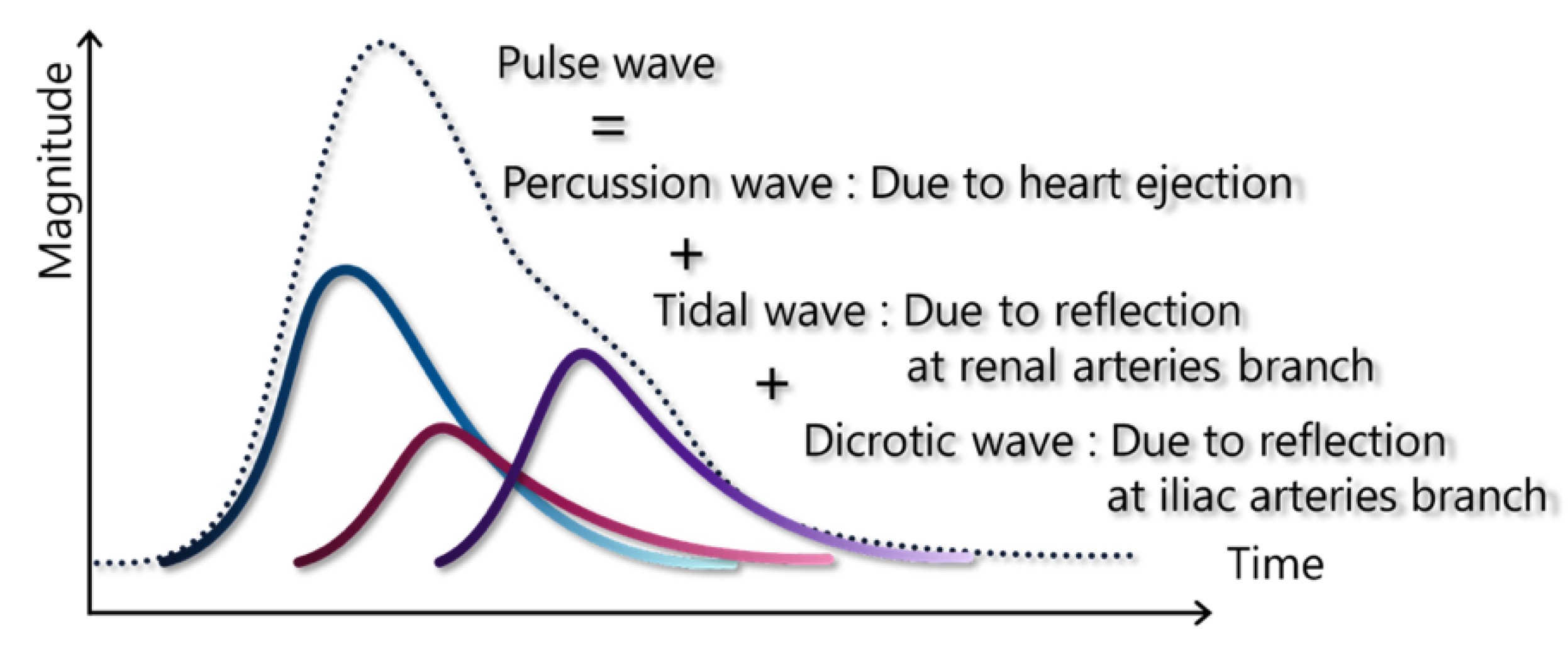
2.1. Pulse Wave Model for Blood Pressure Estimation

In this subsection, we first describe pulse decomposition models used for both sech and Gaussian PDAs. Then, we present the characteristics of the PPG PDA used for regression analysis using the experimental ground truth blood pressure readings.

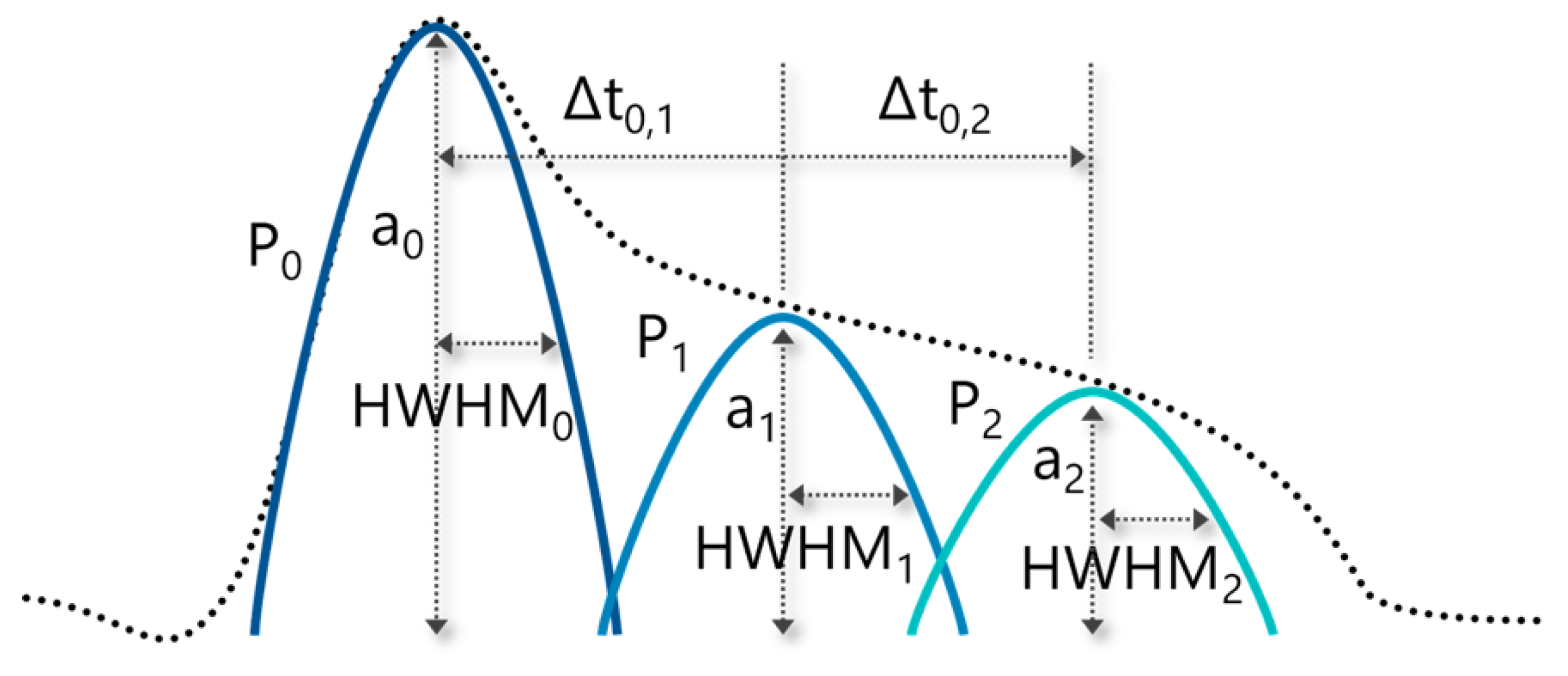
2.1.1. Mathematical Models for Pulse Decomposition Analysis

The PDA model assumes that each pulse wave measured by a PPG device is composed of multiple pulse wave reflections, as illustrated in Figure 1. The multiple reflections do not necessarily propagate at the same speed. Here, we use three-wave decomposition, which has been shown to be adequate for blood pressure estimates using Gaussian decomposition [6]. For this study, we used both the Gaussian PDA (Equation (1)) and our proposed sech PDA (Equation (2)):
f G = a G exp [ ( t μ G ) 2 2 σ G 2 ] .
f S = a S h sech [ t μ S h 2 a S h ] .
where a G and a S h are amplitudes, σ G and σ S h are widths, and μ G and μ S h are the center positions along the time axis of the respective waveforms. The waves in the pulse wave decomposition of Figure 2 can be described by a set of three Gaussian waves, or by three sech waves. These models were used to perform na analysis, described below, to determine between Gaussian waves and sech waves, and which one was better suited to estimate blood pressure by PDA.

2.1.2. Features Extraction from Decomposed Waves Based on Pulse Wave

First, the PPG pulse waves were fitted with Equation (1) and with Equation (2). For curve fitting, after data preprocessing and individual pulse wave separation, we used Matlab’s lsqcurvefit to solve the nonlinear curve approximation by the least-squares method. The fitting of each pulse wave to three sets of Equations, such as Equations (1) or (2), gave 3 sets of parameters. First, the time difference between the peak of the first wave and the peak of the second wave of the three decomposed waves, Δ t 0 , 1 , and the time difference between the peak of the first wave and the peak of the third wave, Δ t 0 , 2 , were obtained as features corresponding to PTT. Next, the amplitude ‘a’ of the waves was used as a feature. The pulse wave amplitude was obtained from each of the three decomposition waves. Finally, the half-width at half-maximum (HWHM) of the waves was also used as a feature. The reason for using the half-width at half-maximum is that it is known that pulse wave strain correlates with blood pressure, and changes in pulse wave strain are thought to affect the half-width [9]. The half-width at half-maximum was also obtained from each of the three decomposition waves. In this study, we investigated the possibility of estimating blood pressure using a total of eight features: the time difference Δ t 0 , 1 , Δ t 0 , 2 from the three decomposed waveforms, the amplitudes a 0 , a 1 , and a 2 of the three waveforms, and the half-width at half-maximums HWHM 0 , HWHM 1 , and HWHM 2 of the three waveforms.

2.1.3. Multiple Regression for the Relationship between the Features and Blood Pressure

To determine the adequacy of the PDA features of PPG for blood pressure estimation, we performed a multiple regression between the features and the ground truth blood pressure. Up to eight features can be used in this study, and the feature combination depends on the number of features used. Since the number of features was small, we decided to adopt the set of features that indicated the best performance in all combinations of the features.

2.2. Dataset Construction for the Verification of Our Proposed Method

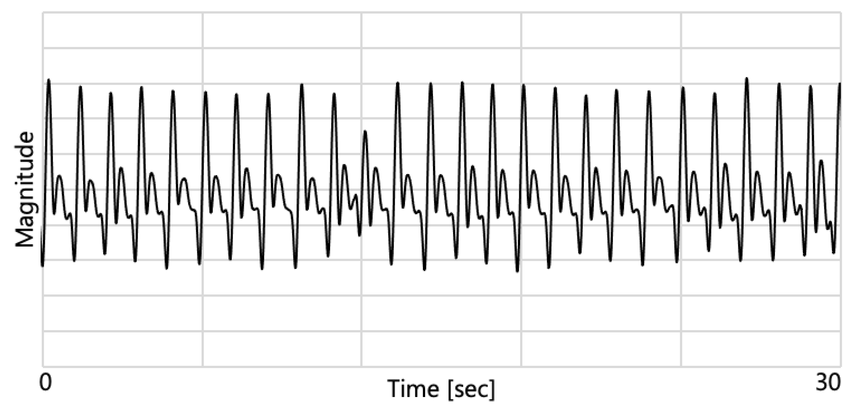
2.2.1. Vital Signs Acquisition

We experimentally constructed a data set by continuously measuring blood pressure using a continuous sphygmomanometer (Finometer MIDI, Finapres Medical Systems), which measures blood pressure with each beat of pulse and pulse wave with a sampling rate of 200 [Hz]. This continuous sphygmomanometer can measure blood pressure non-invasively by attaching a cuff to the fingertip. In addition, we simultaneously acquired the pulse wave, which was measured using photoplethysmography (Procomp/BVP fingertip PPG, 2048 samples per second, with an output sampling rate of 200 samples per second). The subjects in this experiment were 10 adult Japanese volunteer students, aged 22.4 ± 1.7 years (2 females, 8 males). The risks of the exercise were explained to each volunteer both orally and in writing before they consented to the experiment. Since it is necessary to vary the subject’s blood pressure in the experiment, subjects were asked to repeatedly relax and hold their breath for as long as they comfortably could, or up to 60 s. The relaxation phase was placed before and after each breath-holding phase, and was repeated three times.

2.2.2. Data Pre-Processing

Since the measured pulse wave contained noise, pre-processing was necessary. In particular, if the pressure applied to the finger wearing the PPG changed, a trend appeared in the pulse wave, as shown in Figure 3. Therefore, it was necessary to remove the trend. First, trend elimination was performed on the measured pulse wave. For trend elimination, the trend elimination method proposed by Tarvainen et al. was used [11]. Next, a band-pass filter (0.5 to 10 Hz) was applied to the trend-removed pulse wave to remove mainly high-frequency noise. By performing this process, the trend and noise of the pulse wave could be removed, as shown in Figure 4. Next, each subject’s experimental data with a data length of 480 s was divided into 60 segments with a data length of 8 s. In each segment, unitary pulse waveforms were extracted, and the features obtained from the unitary waveforms in the 8-s interval were averaged to be further used for multiple regression. Each unitary pulse waveform was obtained by segmenting the pulse wave based on the position of the detected pulse wave trough. Blood pressure measured with a continuous sphygmomanometer was similarly divided into 60 segments, with a data book of 8 s from one experimental data with a data length of 480 s. In each segment, the mean value of systolic blood pressure was used for multiple regression analysis. Figure 5 shows a box plot with the 60 systolic blood pressures (sbp) of each subject, which are averaged in each window of 8 s.

2.3. The Verification of Our Proposed Method
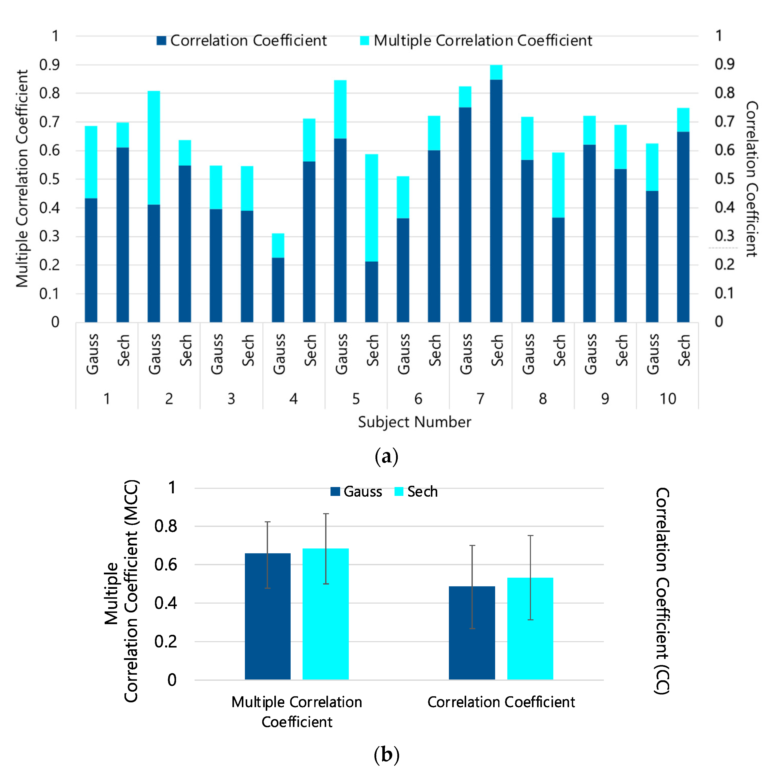
In this study, the two estimation methods based on sech function-based PDA or Gaussian function-based PDA were subjected to two validations: the first was the accuracy of the model for training (regression) with known data, and the second was the accuracy of the model to predict blood pressure (“unknown” data not used for training) with the regression coefficients obtained from the training data.
In addition, two analyses were performed for each validation. The first wanaan analysis using a within-subject model, which did not consider individual differences. The second was an analysis using a between-subjects model, that is, the regression coefficients were obtained using multiple subjects.
First, multiple regression analysis was performed using all subjects’ data without data division. The goodness of fit of the multiple regression analysis was quantified by calculating the multiple correlation coefficients, which determined the extent to which the features achieved a description of blood pressure for all subjects’ data. In this test, two analyses were performed, one for each subject data (within-subject test) and the other for all subject data (between-subjects test). We adopted first-order regression models.
Second, to quantify the estimability for the test data, the Leave One Out method was applied to the dataset, and the correlation coefficient between the ground truth and the estimate was calculated. Similar to the first case, here, two analyses were performed: one for each subject’s data and the other for all subject’s data. The Leave One Out method was used to split the segment data into training data and test data. These data were divided into 59:1 segments by the Leave One Out method for the within-subject model, and into 599:1 segments for the between-subjects model. The Leave One Out method was conducted with the Python programming language library Scikit-learn, which is a machine learning library.
Regarding the selected features, we used the feature set that provided the best performance for each subject’s data. This was because the optimal feature set for each subject could have been different because of individual differences. For verification with the training data, the feature set (function parameters) that provided the best performance was used to determine multiple correlation coefficients. As a result, all features provided the best performance on all subjects’ data. For verification with the test data, the feature set that provided the best performance was used to determine the multiple correlation coefficients. As a result, the features set shown in Table 1 provided the best performance.
Statistical p-values were calculated using t-tests for comparison between two quantities with standard deviations. For the determination of the p-value of the slope of the linear regressions of the ground truth vs. the estimated value of systolic blood pressure, we considered that the null hypothesis was that the slope was zero (no correlation).

3. Results

Multiple regression was performed between PDA (Gaussian and sech) on plethysmographic data and the continuous blood pressure measurement data from the 10 subjects (60 segments of 8 s, for each subject), as discussed in Section 2.
Initially, we studied multiple correlations between BP and PDA parameters independently for each subject. For each subject’s data (60 8-s segments), the average Gaussian PDA and sech PDA parameters in the 8-s segments were used to determine the multiple correlation coefficient against the corresponding average BP ground truth in the same segments (Figure 6a). Moreover, in Figure 6a, using similar data segmentation and multiple regression, we show the correlation coefficient of the Leave One Out (59:1) BP prediction vs. the corresponding average BP ground truth in the segment left out. This correlation coefficient was thus calculated using 60 data points per volunteer, since the Leave One Out (LOO) procedure was executed comprehensively for all 8-s segments of each subject. In Figure 6a, all results are calculated on an individual-by-individual basis.
Figure 7 shows a scatterplot with all the 600 data points (for all 10 subjects), where the BP was predicted using the regression model learned with each subject data individually. We call this “training data”. Note that the Gaussian PDA (R2 = 0.77, p = 0.0000) underperformed compared with the prediction power of the sech PDA (R2 = 0.81, p = 0.0000).
Figure 8 is similar to Figure 7, but each one of the 600 data points was generated by an LOO prediction (‘test data’), with an underlying regression model learned for each subject data individually. For each subject, 60 data points were generated by LOO 59:1. Again, the Gaussian PDA (R2 = 0.58, p = 0.0000) underperformed compared with the prediction power of the sech-PDA (R2 = 0.76, p = 0.0000).
To further investigate possible performance differences between Gaussian PDA and sech PDA, we reanalyzed the data produced for Figure 6a. First, we averaged the multiple correlation coefficients, and the correlation coefficient, both from Figure 6a, which were determined independently for each one subject. The result of such an average is shown in Figure 6b. There was no statistically significant difference between the performance of the Gaussian PDA and the sech PDA by this analysis.
Finally, Figure 9 shows multiple regression and correlation coefficients (from LOO) conducted on the data of all the subjects processed together (600 segments). Notice in Figure 9, there is a reduction in the multiple correlation coefficient, and in the correlation coefficient compared to regressions with the data of only one subject at a time, as in Figure 6b. Again, there was no statistically significant difference between the performance of Gaussian PDA and the sech PDA. This seems to indicate that, for long timeframes, Gaussian PDA and sech PDA, on average, converge to the same prediction power.
For completeness, we show in Figure 10 mean squared errors (MSE) between the original pulse wave and the reproduced wave based on Gaussian PDA or Sech PDA in each subject (for all data regressions, analogous to Figure 7). Although Gaussian PDA showed a slightly better fit (slightly lower MSE), Figure 8 (leave one out prediction) makes it evident that the sech PDA better explained BP. The results of Figure 10 may suggest that the sech PDA was a better fit for the pulse contour region, and was more relevant for estimating blood pressure [16]. The small MSE values come from having normalized the PPG pulse amplitudes to one, for both Gaussian PDA and sech PDA, for a fair comparison.
We also conducted a multiple regression using only the coefficient’s ratio a2/a1, as suggested by [3]. Specifically, we conducted multiple regression with each subject data, for all ten subject data, to calculate a multiple correlation coefficient, and averaged the ten multiple correlation coefficients. For Gaussian PDA the multiple correlation coefficients gave 0.20 ± 0.17 (mean ± standard deviation), with the range 0.031, 0.50, and for the sech PDA, the multiple correlation coefficients gave 0.26 ± 0.17 (mean ± standard deviation), with range 0.034, 0.59. No statistically significant difference was found between the Gaussian PDA and the sech PDA results, but the low multiple correlation coefficient discourages the use of the coefficient’s ratios for PDA-based BP estimation.

4. Discussion

Here, we compared models of blood pressure description by sech PDA and by Gaussian PDA, and their characteristics. Gaussian PDA showed the best performance in the literature on PDA blood pressure measurement [8]; however, sech PDA has not been tested in the literature for blood pressure estimates. Our results showed that the use of sech PDA instead of Gaussian PDA could lead to more accurate and robust blood pressure measurement.
Our main results are shown in Figure 7 and Figure 8. Sech PDA better explains BP (78% vs. 58%, p = 0.0000) than Gaussian PDA, in our data. Our data is challenging because it presented a large variation in BP in 8 min (Figure 5). To prevent possible issues in the comparison between the sech and the Gaussian function PDA, in our tests, we did not complete a full prediction, but instead performed a Leave One Out model test, in 8-s intervals. The choice of Leave One Out and the choice of the 8-s intervals were arbitrary.
Results of Figure 6 and Figure 9 do not show statistically significant differences between sech PDA and Gaussian PDA for timeframes (averages) of the order of 80 minutes, with averages also between individuals. This was expected since Gaussian PDA is a good method for BP estimates. In addition, our results of Figure 7 and Figure 8 imply that sech PDA correlated at least as well with blood pressure as Gaussian PDA.
We also found that multiple regression between PDA features and blood pressure, using all features, achieved higher accuracy compared to simply using one feature—which was not surprising. We had a higher accuracy with all features than the other combinations of features in the multiple correlation coefficients. Arithmetic operations (such as the ratio index a2/a1 used in [13]) gave a lower (worse) multiple correlation coefficient for all subject data. We believe this behavior was caused by the dimensionality loss in arithmetically combining multiple features, worsening the pulse contour description.
Figure 10 shows that the mean square error of the PDA fits was slightly lower for Gaussian PDA than for sech PDA. Because sech PDA gave a better correlation with blood pressure, we speculated that if sech did not provide a better fit to the pulse than the Gaussian function, this was due to the difference in the importance of different regions of pulse wave contour for blood pressure estimates [16]. Pulse wave contours reproduced by Gaussian PDA and sech PDA fit different contours, despite the same goodness of fit. Such analysis is beyond the scope of the present paper.
An important early study based on Gaussian PDA [7] found R2 correlations with central line catheter SBP and DBP to be 0.92 and 0.78, respectively. By comparison, our study shows the R2 was 0.58 for SBP based on the Gaussian PDA (Figure 8a), and 0.76 for SBP based on the sech PDA (Figure 8b), with ground truth reference BP peripherally measured in the finger. While [7] used data from 38 male and 25 female patients of 62.7 ± 11.5 years old, our study used data of healthy volunteers 22.4 ± 1.7 years old (8 males and 2 females) whose blood pressures varied by up to 60% during data collection, which made the prediction in our case more challenging. More detailed tests on clinical datasets will be the subject of future work.
Among the limitations in our study was the windowing process, which averaged the feature values and blood pressure in time intervals of 8 s. It is possible that the mean value of the parameters in this window could not accommodate for a wide variation of blood pressure. The windowing process also brought a second limitation: the 8-s interval of the moving window limited “real-time” blood pressure estimates at the beginning of the measurement. Sudden changes in BP may have limited the response of the finger cuff continuous BP meter, limiting the accuracy of our study compared with a central line catheter BP meter. Moreover, we used the mean values of the BP and the PDA parameters in each 8-s segment. If the statistical distribution of values in the segments were skewed, the prediction was poor, and the median or other metric would be more appropriate. Another limitation in this study was that, to simplify the analysis, we focused only on the systolic blood pressure.
Finally, we will consider future work. Blood pressure depends on an individual’s weight, height, and body mass index [17]. There is room to consider this information in the description of blood pressure using PDA. In addition, it may be possible to estimate blood pressure using more individually appropriate models and methods by grouping subjects based on their biometric information and creating estimation models for each group. This point also needs to be verified. Furthermore, the optimal number of sech-waves on a pulse contour needs to be investigated, since the optimal number of waves to be used for PDA may vary [18].

5. Conclusions

In this study, we proposed a method for decomposing the pulse wave into three hyperbolic orthogonal waves and estimating blood pressure based on the features obtained from the waves. This method was applied to a dataset constructed by measuring pulse waves while varying blood pressure. The multiple regression based on sech PDA showed equal or higher accuracy than multiple regressions based on Gaussian PDA (Supplementary Materials).

Supplementary Materials

The data produced for this paper are available at https://github.com/iuchik/est_bp_with_pda.

Author Contributions

Conceptualization, R.T., R.P.d.S. and G.C.C.; formal analysis, T.N., R.T., M.T. and K.I.; investigation, T.N., R.T. and K.I.; methodology, T.N., R.T. and R.P.d.S.; software, T.N., R.T., R.P.d.S. and K.I.; supervision, N.T. and G.C.C.; validation, K.O.-O., N.T. and G.C.C.; writing—original draft, K.I.; writing—review and editing, G.C.C., K.O.-O. and N.T. All authors have read and agreed to the published version of the manuscript.

Funding

The authors acknowledge funding from JSPS KAKENHI Grant Number 19K12750, Japan. This study was financed in part by the Coordenação de Aperfeiçoamento de Pessoal de Nível Superior—Brazil (CAPES)—Finance Code 001.

Institutional Review Board Statement

This study was approved by the Medical Ethics Committee of Kanazawa University, approval no.2018-154 (2912). and conducted in accordance with the Declaration of Helsinki.

Informed Consent Statement

Informed consent was obtained from all subjects involved in the study.

Conflicts of Interest

The authors declare no conflict of interest.

References

  1. Vrijkotte, T.G.; Van Doornen, L.J.; De Geus, E.J. Effects of work stress on ambulatory blood pressure, heart rate, and heart rate variability. Hypertension 2000, 35, 880–886. [Google Scholar] [CrossRef]
  2. Zheng, W.; Zhang, S.; Deng, Y.; Wu, S.; Ren, J.; Sun, G.; Yang, J.; Jiang, Y.; Xu, X.; Wang, T.; et al. Trial of intensive blood-pressure control in older patients with hypertension. N. Engl. J. Med. 2021, 385, 1268–1279. [Google Scholar] [CrossRef] [PubMed]
  3. McGhee, B.H.; Bridges, E.J. Monitoring arterial blood pressure: What you may not know. Crit. Care Nurse 2002, 22, 60–79. [Google Scholar] [CrossRef]
  4. Alpert, B.S.; Quinn, D.; Gallick, D. Oscillometric blood pressure: A review for clinicians. J. Am. Soc. Hypertens. 2014, 8, 930–938. [Google Scholar] [CrossRef] [PubMed]
  5. Drzewiecki, G.; Hood, R.; Apple, H. Theory of the oscillometric maximum and the systolic and diastolic detection ratios. Ann. Biomed. Eng. 1994, 22, 88–96. [Google Scholar] [CrossRef]
  6. Couceiro, R.; Carvalho, P.; Paiva, R.P.; Henriques, J.; Quintal, I.; Antunes, M.; Muehlsteff, J.; Eickholt, C.; Brinkmeyer, C.; Kelm, M.; et al. Assessment of cardiovascular function from multi-Gaussian fitting of a finger photoplethysmogram. Physiol. Meas. 2015, 36, 1801. [Google Scholar] [CrossRef] [PubMed]
  7. Baruch, M.C.; Kalantari, K.; Gerdt, D.W.; Adkins, C.M. Validation of the pulse decomposition analysis algorithm using central arterial blood pressure. Biomed. Eng. Online 2014, 13, 96. [Google Scholar] [CrossRef] [PubMed] [Green Version]
  8. Teng, X.F.; Zhang, Y.T. Continuous and noninvasive estimation of arterial blood pressure using a photoplethysmographic approach. In Proceedings of the 25th Annual International Conference IEEE Engineering Medicine and Biology Society, Cancun, Mexico, 17–21 September 2003; pp. 3153–3156. [Google Scholar]
  9. Suzuki, S.; Oguri, K. Cuffless and and non-invasive systolic blood pressure estimation for aged class by using a photoplethysmography. In Proceedings of the 2008 30th Annual International Conference of the IEEE Engineering Medicine and Biology Society, Vancouver, BC, Canada, 20–25 August 2008; pp. 1327–1330. [Google Scholar]
  10. Kurylyak, Y.; Lamonaca, F.; Grimaldi, D. A neural network-based method for continuous blood pressure estimation from a PPG signal. In Proceedings of the 2013 IEEE International Instrumentation and Measurement Technology Conference (I2MTC), Minneapolis, MN, USA, 6–9 May 2013; pp. 280–283. [Google Scholar]
  11. Yoon, Y.Z.; Kang, J.M.; Kwon, Y.; Park, S.; Noh, S.; Kim, Y.; Park, J.; Hwang, S.W. Cuff-Less Blood Pressure Estimation Using Pulse Waveform Analysis and Pulse Arrival Time. IEEE J. Biomed. Health Inform. 2017, 22, 1068–1074. [Google Scholar] [CrossRef] [PubMed]
  12. Jeong, I.C.; Finkelstein, J. Introducing contactless blood pressure assessment using a high speed video camera. J. Med. Syst. 2016, 40, 77. [Google Scholar] [CrossRef] [PubMed]
  13. Zheng, Y.L.; Yan, B.P.; Zhang, Y.T.; Poon, C.C. An armband wearable device for overnight and cuff-less blood pressure measurement. IEEE Trans. Biomed.-Med. Eng. 2014, 61, 2179–2186. [Google Scholar] [CrossRef] [PubMed]
  14. Sawada, Y.; Tanaka, G.; Yamakoshi, K.I. Normalized pulse volume (NPV) derived photo-plethysmographically as a more valid measure of the finger vascular tone. Int. J. Psychophysiol. 2001, 41, 1–10. [Google Scholar] [CrossRef]
  15. Tarvainen, M.P.; Ranta-Aho, P.O.; Karjalainen, P.A. An advanced detrending method with application to HRV analysis. IEEE Trans. Biomed. Eng. 2002, 49, 172–175. [Google Scholar] [CrossRef] [PubMed]
  16. Ruiz-Rodríguez, J.C.; Ruiz-Sanmartín, A.; Ribas, V.; Caballero, J.; García-Roche, A.; Riera, J.; Nuvials, X.; de Nadal, M.; de Sola-Morales, O.; Serra, J.; et al. Innovative continuous non-invasive cuffless blood pressure monitoring based on photoplethysmography technology. Intensive Care Med. 2013, 39, 1618–1625. [Google Scholar] [CrossRef] [PubMed]
  17. De Souza, R.P.; Janke, B.; Cardoso, G.C. Decomposição de pulsos fotopletismográfico para redução da incerteza do Tempo de Trânsito. Rev. Bras. Física Médica 2020, 14, 546–554. [Google Scholar]
  18. Tang, Q.; Chen, Z.; Ward, R.; Elgendi, M. Synthetic photoplethysmogram generation using two Gaussian functions. Sci. Rep. 2020, 10, 13883. [Google Scholar] [CrossRef] [PubMed]
Figure 1. Pulse decomposition into three constituent waves (adapted from [14,15]).
Applsci 12 01798 g001
Figure 2. PPG pulse decomposition into three constituent waves and extracted features.
Applsci 12 01798 g002
Figure 3. Original pulse wave.
Applsci 12 01798 g003
Figure 4. Processed pulse wave.
Applsci 12 01798 g004
Figure 5. Box plots with 60 systolic blood pressure (sbp) for each subject. Each sbp point is the average of an 8-s window.
Applsci 12 01798 g005
Figure 6. Multiple correlation coefficients for each subject data as the training data and the correlation coefficients calculated by Leave One Out for each subject dataset. (a) Results for each subject independently. (b) Mean value of results from (a). For the group, the differences between the Gaussian and sech results are not statistically significant.
Applsci 12 01798 g006
Figure 7. Scatter plots for each subject data as training data in multiple regression. (a) Result based on Gaussian PDA. (b) The result based on sech PDA multiple regression was performed with 60 simultaneous 8-s segments of continuous systolic blood pressure vs. PPG pulse decomposition features for each subject data. Each scatterplot contains 600 data points. For both plots, p = 0.0000.
Applsci 12 01798 g007
Figure 8. Scatter plots for each subject data as test data by multiple regression using Leave One Out. (a) Result based on Gaussian PDA. (b) Result based on sech PDA. In Leave One Out, we estimated systolic blood pressure with an 8-s segment based on the multiple regression model learned with the other segments of the subject data, and we repeated the process to test all 60 segments data comprehensively. Each scatterplot contains 600 data points. For both plots, p = 0.0000.
Applsci 12 01798 g008
Figure 9. The multiple correlation coefficients for all the subjects’ data and the correlation coefficients for all the subjects’ data with Leave One Out analysis. The reduction in the coefficients compared to Figure 7 implies that PDA for each individual must be calibrated by an independent regression.
Applsci 12 01798 g009
Figure 10. Mean squared error between the original pulse wave and the reproduced wave based on Gaussian PDA or sech PDA in each subject.
Applsci 12 01798 g010
Table 1. The combination of the features used in the Leave One Out test.
Combination of Features
Subject NumberSech-PDAGaussian-PDA
1Δt0,1, FWHM2Δt0,2, a1, a2, FWHM1, FWHM2, FWHM3
2a3, FWHM1, FWHM2, FWHM3Δt0,2, FWHM1
3Δt0,1, a1, a2, FWHM2Δt0,1, a2
4Δt0,1, a1, a2, FWHM1Δt0,1, FWHM1
5FWHM2, FWHM3Δt0,1, FWHM1, FWHM2, FWHM3
6Δt0,1, a2, a3, FWHM3Δt0,1, Δt0,2, a1, a2, FWHM1
7a1, a3, FWHM2, FWHM3Δt0,1, FWHM3
8Δt0,1, a3Δt0,1, a1, a2, a3, FWHM1, FWHM2, FWHM3
9Δt0,1, a2, FWHM1, FWHM2Δt0,1, a2, FWHM1, FWHM2
10Δt0,1, Δt0,2, a2, FWHM1, FWHM2Δt0,1, a1, a2, FWHM2, FWHM3
alla2, FWHM1, FWHM2Δt0,1, Δt0,2, a2, FWHM2, FWHM3
Publisher’s Note: MDPI stays neutral with regard to jurisdictional claims in published maps and institutional affiliations.

