
Adaptive Deconvolution-Based Stereo Matching Net for Local Stereo Matching


1
School of Information Science and Engineering, Shandong University, Qingdao 266237, China
2
College of Geomatics, Shandong University of Science and Technology, Qingdao 266590, China
3
School of Control Science and Engineering, Shandong University, Jinan 250061, China
*
Author to whom correspondence should be addressed.
Appl. Sci. 2022, 12(4), 2086; https://0-doi-org.brum.beds.ac.uk/10.3390/app12042086
Submission received: 9 January 2022
/
Revised: 28 January 2022
/
Accepted: 29 January 2022
/
Published: 17 February 2022
(This article belongs to the Special Issue Computer Vision and Pattern Recognition Based on Deep Learning)
Abstract
:In deep learning-based local stereo matching methods, larger image patches usually bring better stereo matching accuracy. However, it is unrealistic to increase the size of the image patch size without restriction. Arbitrarily extending the patch size will change the local stereo matching method into the global stereo matching method, and the matching accuracy will be saturated. We simplified the existing Siamese convolutional network by reducing the number of network parameters and propose an efficient CNN based structure, namely adaptive deconvolution-based disparity matching net (ADSM net) by adding deconvolution layers to learn how to enlarge the size of input feature map for the following convolution layers. Experimental results on the KITTI2012 and 2015 datasets demonstrate that the proposed method can achieve a good trade-off between accuracy and complexity.
1. Introduction
Three-dimensional scene reconstruction is important in autonomous driving navigation, virtual/augmented reality, etc. The texture/color information of a scene can be captured directly by cameras, whereas the scene geometry (especially the depth information) cannot be obtained easily. There are two ways to obtain the depth information, one is a direct measurement, another is binocular vision. Special devices, like laser detectors and millimeter-wave radars, are needed for direct measurement. Besides the direct measurement, depth information can also be obtained by binocular vision-based stereo matching indirectly. With the great development of high- performance computing devices, the depth information will be estimated easily by using the captured left and right view images without additional expensive devices.
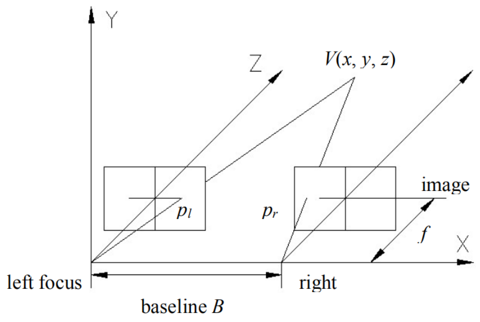
Figure 1 shows a typical binocular camera model [1]. The two-camera centers are placed on the same horizontal line with a baseline of . Usually, the center of the left camera is set to be the base point, that is, left focus. The optical axes of the two cameras are parallel, and the optical axis of the left camera is denoted as the axis . The image plane of the two cameras is parallel with the plane which is perpendicular to the axis . Suppose a point in the 3D space, which can be projected onto the pixel position and of the image plane. The discrepancy between and is defined as the disparity, i.e., By using the principle of similar triangles, the depth of the point can be calculated by:
where represents the focal length of the camera. The value of and can be calculated by:
where and are the horizontal and vertical coordinates of the point on the left image plane. Because the baseline and the focal length can be obtained after camera calibration [2], only the disparity should be calculated to obtain the depth information of a scene.
Stereo matching [3] between the left and the right images can be used to calculate the disparity. Generally speaking, there are three kinds of stereo matching algorithms, i.e., local minimization-based matching, regional minimization-based matching, and global minimization-based matching. With a given matching error function, the local minimization-based matching algorithms are conducted by finding the disparity that can result in local minima for a pixel. Typical algorithms are cross-based local stereo matching with orthogonal integral images [4], local stereo matching with improved matching cost [5], etc. The regional minimization-based matching assumes that the disparities of pixels in a texture/color region can be modeled by a linear function. By using the initial disparities that are obtained from local minimization-based matching, the disparities of the pixels in each region can be modified by regression [6]. The basic concept of global minimization-based matching is to estimate the disparities of all the pixels directly by modelling and solving a global energy function according to global optimization [7]. Typical global matching algorithms are dynamic programming-based algorithm [8], a belief propagation algorithm [9,10], a graph cut-based algorithm [11,12] and so on. There are different merits and demerits for each kind of algorithm. The complexity of the local minimization-based algorithms is very small, but the accuracy is somewhat not good enough. The global minimization-based algorithms usually give better results than the local minimization-based algorithms, but the complexity is very high. Besides, the boundary effect usually occurs because the global energy function cannot deal with the local texture and depth variations in the scene. The regional minimization-based algorithms seem to exploit the merits of local and global minimization-based algorithms simultaneously, but additional image segmentation is introduced, which increases the complexity.
Recently, because of the excellent performance in dealing with computer vision problems, convolutional neural network (CNN) has also been used for stereo matching [13]. The CNN-based stereo matching algorithms can also be divided into two kinds. One is the end-to-end training-based methods, which usually require relatively large network parameters [14,15], and the other is to use CNNs to extract compact features of blocks in the left and the right images for further matching, a kind of network that is usually simpler than the former. Academically, we usually understand it by analogy with simase convolution network, in contrast to the pseudo simase network, we only need one set of network parameters [16,17,18,19].
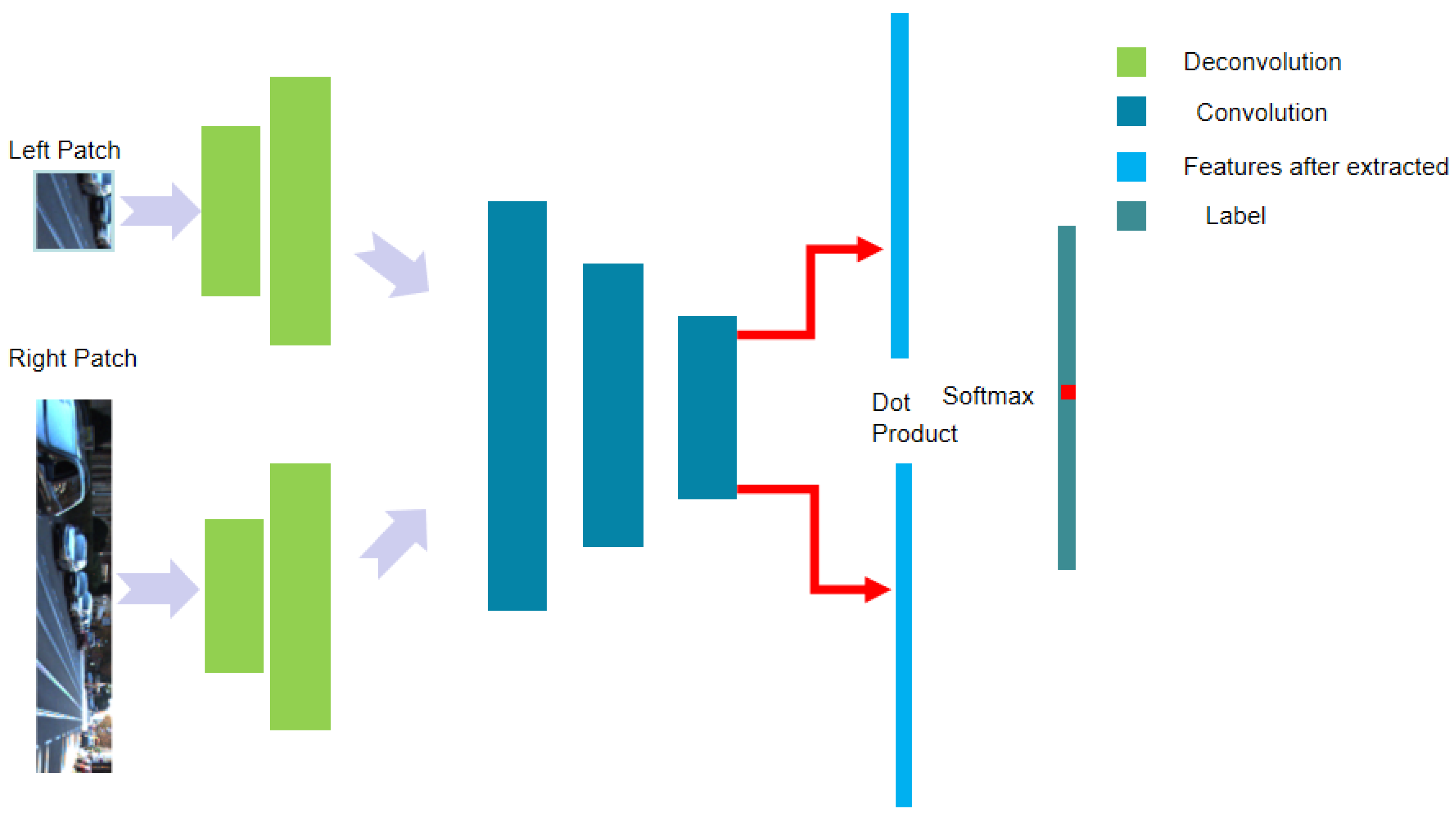
In this paper, we propose an improved CNN-based local matching algorithm. Specifically, to efficiently extract the patch features, we add a deconvolution module in front of the network to learn how to enlarge the size of the input image patches. The de-convolved features of the left and the right view image patches are further fed into the successive convolutional layers with max-pooling to obtain compact features. Afterwards, these compact features are put together by dot product operation to generate a one-dimensional feature. Finally, softmax activation is performed based on the one-dimensional feature to estimate the disparity of the central pixel of the input left view image patch. Experimental results in the KITTI2012 and 2015 datasets show that more accurate disparities can be obtained by the proposed method.
2. Related Work
Traditional stereo matching algorithms mainly include SGM (Semi global matching [20], BM (Block Matching) [21], GC (Graph Cut) [22], BP (Belief Propagation) [10] and DP (Dynamic Programming) [23]. In recent years, apart from the CNN-based stereo matching algorithms, the end-to-end method has also been developed well. N. Mayer et al. [24] created a large end-to-end deep neural network with the synthetic dataset. Dispnet. J. Pang et al. [25] proposed a two-stage coarse end-to-end model to refine the convolutional network for stereo matching. Recently, Khakis [26] proposed an end-to-end neural network that used the stacked hourglass backbone and increased the number of 3D convolutional layers for cost aggregation. However, the end-to-end method usually needs large memory and possesses large computational complexity, and it is hard to converge [27].
For the CNN-based local matching algorithm, A. Geiger et al. [28] built a prior for the disparity to reduce the matching ambiguities of the remaining points. Melekhov et al. [29] created two channels local window with conventional confidence features. The features and disparity patches were trained by CNN simultaneously. Chang et al. [15] proposed a pyramid stereo matching network, namely PSM-Net. The network structure consists of two main modules: spatial pyramid pooling and 3D CNN. It can fully exploit context information for finding correspondence in ill-posed regions. J. Zbontar, et al. [16] proposed a binary classification neural network with supervised training to calculate the matching error with small image patches. Xiao Liu et al. [17] proposed using dilated convolution in the CNN to preserve the features of different scales so that better matching accuracy can be achieved. Compared to traditional convolution, the advantage of dilated convolution is that it can obtain a larger receptive field under the same convolution kernel size. However, too much dilated convolution will lead to too large a network structure and increase redundant information. Luo et al. [18] proposed a stereo matching algorithm by using the twin convolutional networks with shared weights in the left and the right network layers. In this method, the size of image patches ranges from 9 × 9 to 37 × 37. By using the constant size of the convolution kernel and the limited number of layers, the inference time for an image with resolution of 375 × 1275 is only 0.34 s. To improve the matching accuracy of the boundary and the low-texture regions, Feng et al. [27] proposed a deeper neural network with a larger kernel size (such as 17 × 17), while the input images are up-sampled to two times.
In summary, to achieve higher accuracy, the patch size is usually enlarged. But larger patch size also entails larger computational complexity. Moreover, the disparity map size decreases with the increase of the input patch size. For example, in the case that the original image size is 375 × 1242, it will be 347 × 1216, when using the network trained with an input patch size of 29 × 29. When the input patch size is 45 × 45, it will change into 331 × 1198. For the missing pixels at the edge of the image, it’s disparity value is derived from the outermost layer of the disparity map. Besides, there is also an upper bound of the accuracy increment when increasing the input patch size. The above conclusions will be experimentally verified at the end of paper In this paper, we expand the size of the image patch by deconvolution layers instead of using naive up-sampling methods and then obtain better results.
3. Proposed Method
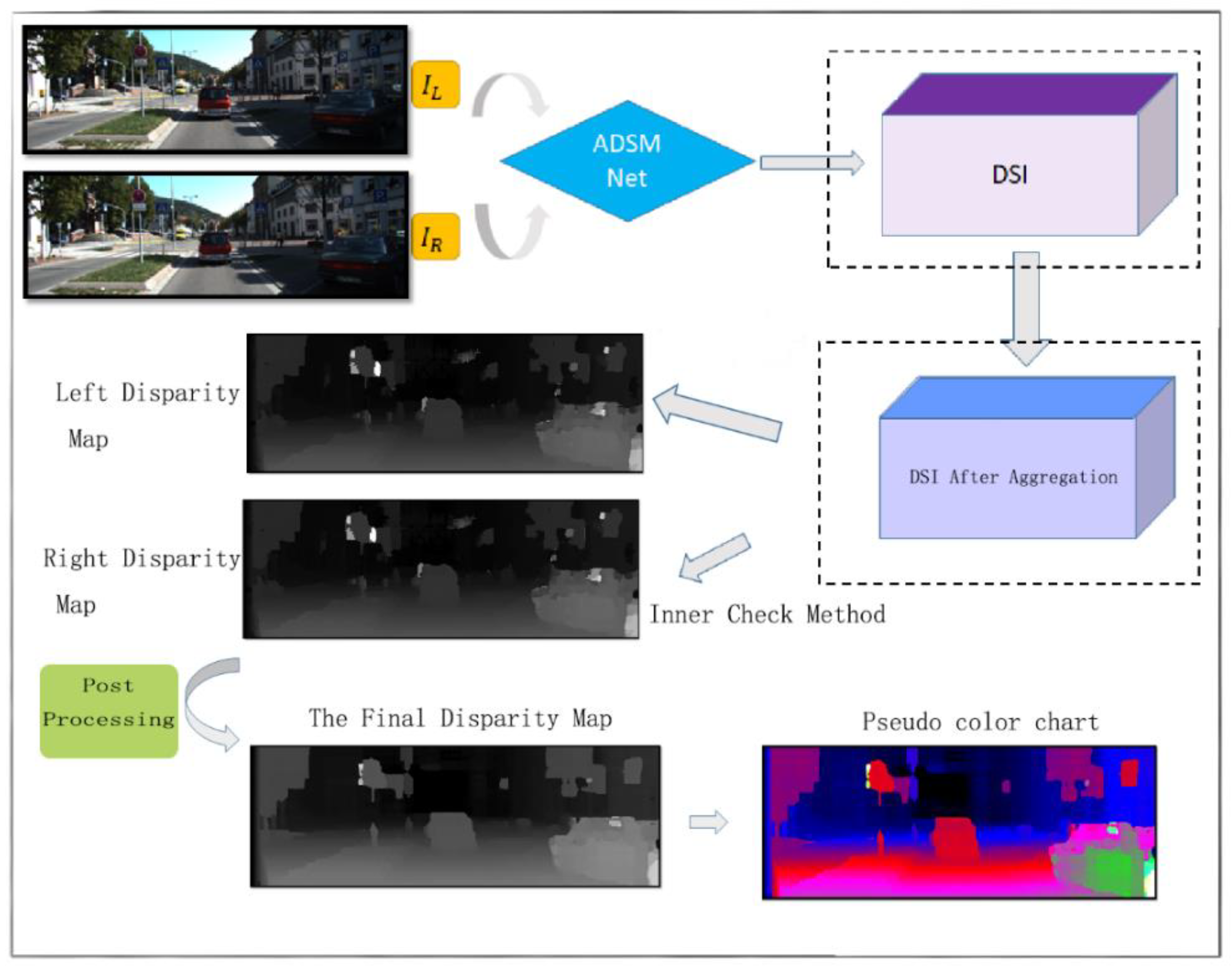
We propose a type of CNN neural network with deconvolution layers [30] to adaptively expand the size of the input patches by referring to the GA-Net feature extraction. We introduce deconvolution at the beginning of the convolutional network and then perform the convolution operation. Deconvolution plays the role of up-sampling. The feature size after deconvolution is larger than the feature size before deconvolution. The backbone of the proposed network is based on the Siamese neural network [31] and MC-CNN network [19], and we refer to the previous part of MC-CNN and combine the network architecture with the Siamese neural network. The basic structure of the proposed network is shown in Figure 2. As can be seen, the overall network structure can be divided into four modules: image patch input module, deconvolution module, convolution module with dot product, and the Softmax-based loss calculation module. In the process of post-processing, we use the internal check method for checking the left and the right consistency, and use the ray filling method for filling invalid pixels. The flow chart of the overall algorithm is shown in Figure 3.
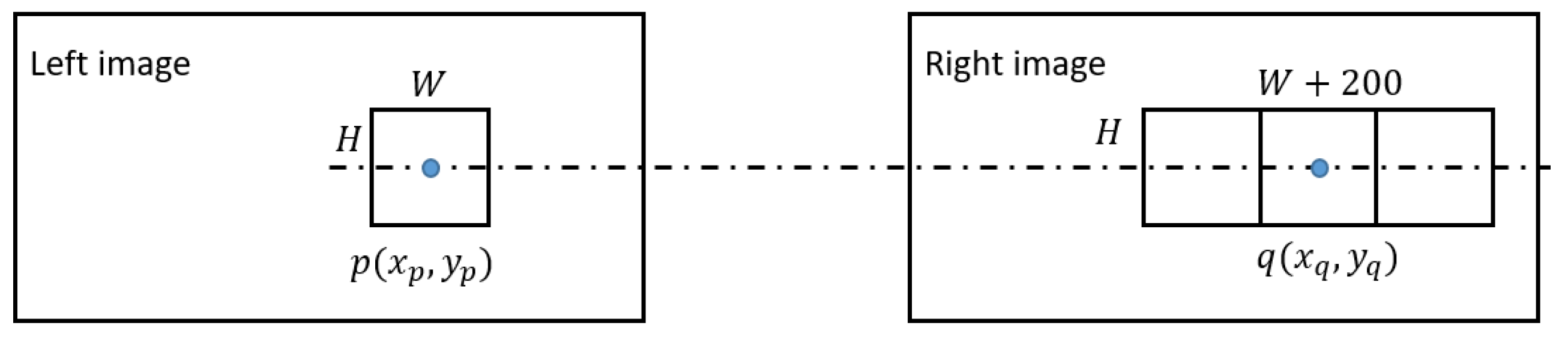
Image patch input module: Two image patches, denoted by and respectively, are input into the neural network, where the superscripts “” and “” denote the left and the right image patch, the subscripts “” and “” represent the size of the two image patches, is the horizontal position of central pixel in the left image patch, and is the horizontal position of a pixel in the central line of the right image patch. The aim of the neural network is to determine whether the left image patch can be matched by a sub-patch with a size of in the right image patch, as shown in Figure 4.
3.1. Deconvolution Module
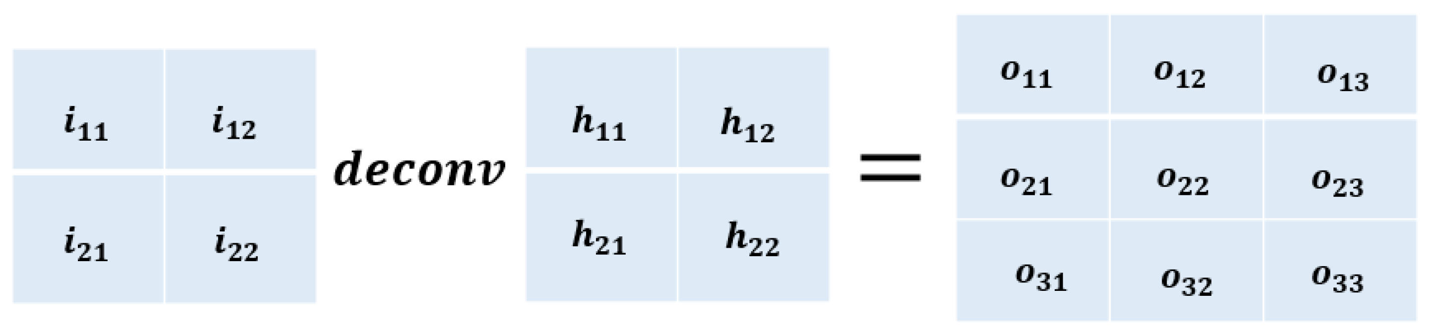
As shown in Figure 5, let the input vector that is reshaped from a matrix of the deconvolution operation be , the output () vector that can be reshaped to a matrix of the deconvolution operation can be written as:
where the subscript “DC” means deconvolution, denotes the parameter matrix of the deconvolution operation,
For the case of multi-deconvolution layers, the output of the deconvolution layer can be represented as:
where, the , …, and are parameters that should be learnt.
Convolution module: The aim of the convolution module is to extract compact features of the left and the right image patches for further matching. As introduced in the deconvolution module, the input vector, the output vector, and the convolution operation can be expressed by , , and ,
For the case of multi-convolutional layers, the output of convolution layer can be represented as:
where, the , …, and are the parameters of each layer that should be learnt.
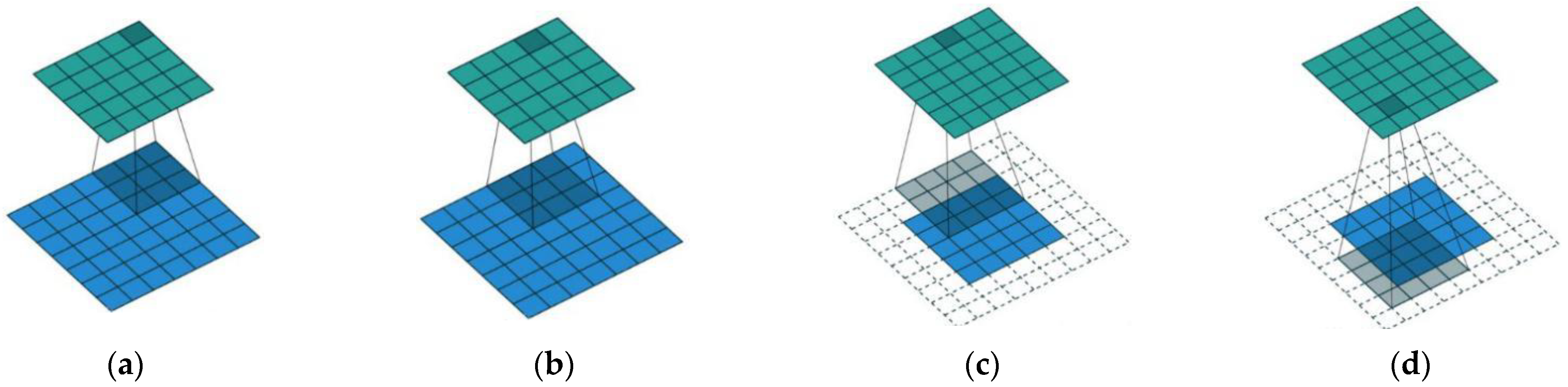
Figure 6 shows the difference between convolution and deconvolution operations. The calculation relationship of the size of the convolutional network is:
while the calculation relationship of the size of the deconvolution network is:
where represents the output feature size, represents the input feature size, represents the step size, represents the fill size, and represents the convolution kernel size. In the convolutional neural network, the number of channels of the input feature is , the number of channels of the output feature map is , and the size of the convolution kernel is . Then the number of parameters of the convolutional layer is . If the batch normalization structure is adopted, [25] should be omitted.
As shown in Figure 2, the left and the right image patch pass through their respective network branches. Each network branch contains different sizes of convolutional kernels. The size of the convolutional kernels of each layer varies according to the size of the previous layer. Each layer is then followed by a rectified linear units (ReLU) layer and batch normalization (BN) function except for the last layer. The output of the two branches are respectively, where:
and
. Finally, the following dot product layer is adopted.
to generate a vector to indicate the matching degree of each possible disparities between the two image patches.
3.2. Softmax-Based Loss Calculation Module
In this module, we use Softmax classifier equipped by cross-entropy loss function to calculate the loss of each disparity. Note that there are 201 possible disparities in the proposed method. For each possible disparity , the softmax function can be written to be:
where denotes the probability of . The outputs of all the possible disparities is then generated to be an output vector . The cross-entropy loss can be calculated by:
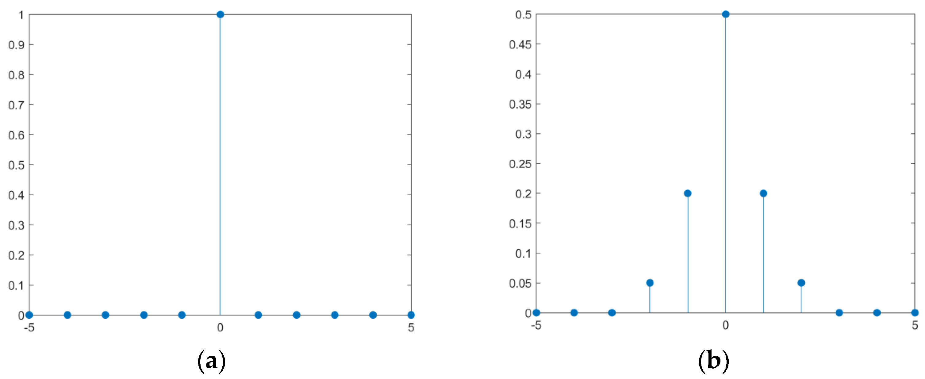
where denotes the current network parameters, is the ground truth label of each possible disparities. The ground truth label can be defined as a vector with only a single “1” element and “0” for all the other elements, where the position of the “1” element corresponds to the actual disparity, as shown in Figure 7a. To be more flexible, we define the to be:
where represents the groundtruth disparity value, as shown in Figure 7b. The training procedure is to find the optimal network parameter to minimize the cross-entropy loss of (18).
3.3. Post-Processing
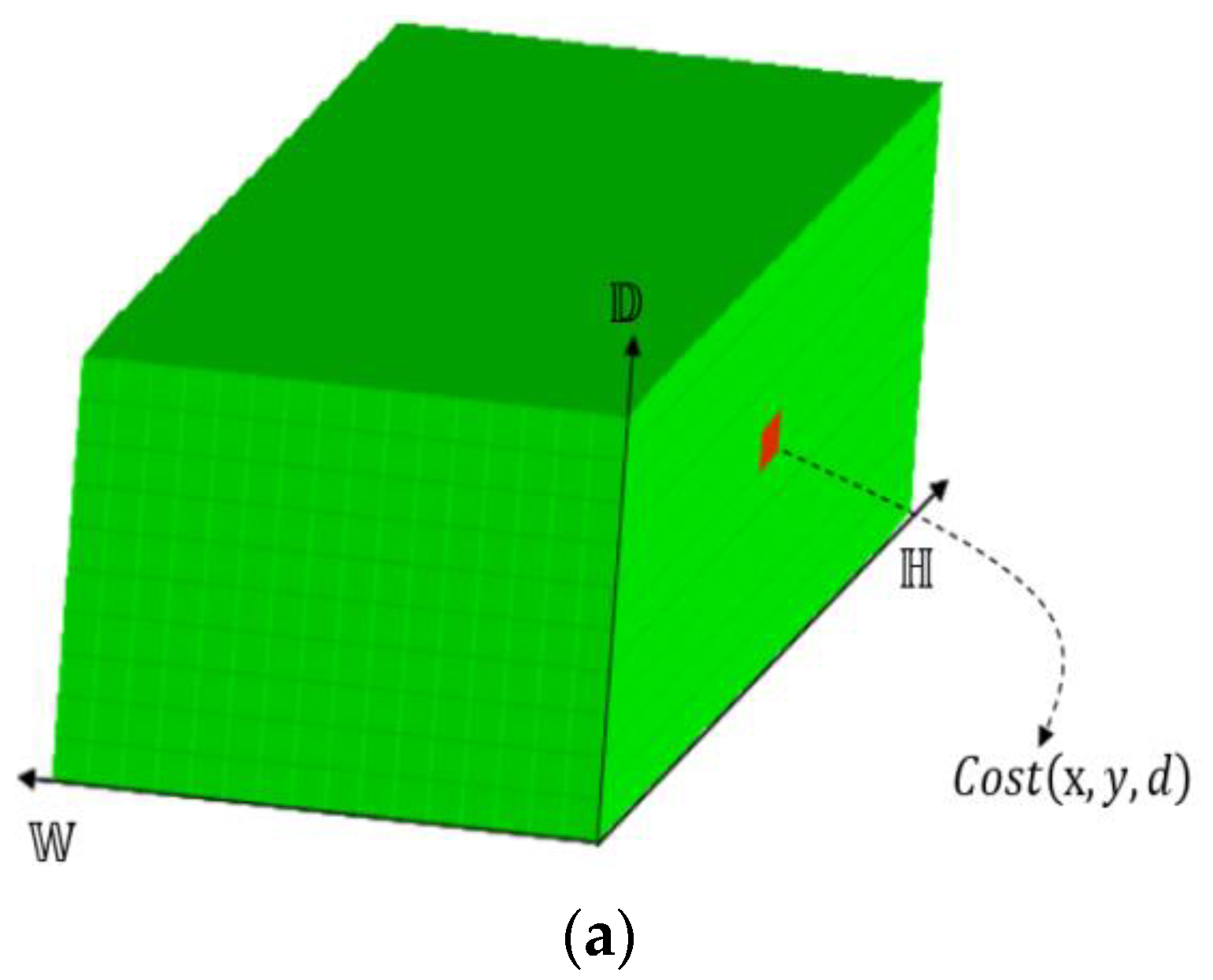
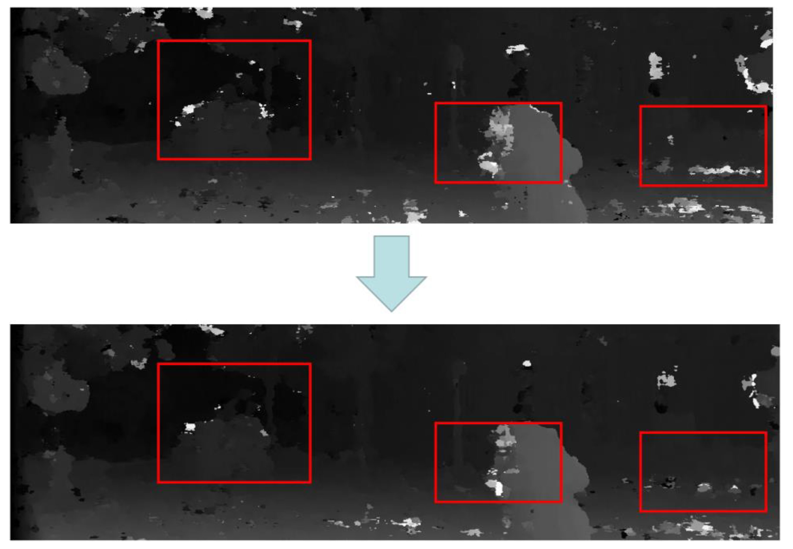
In the training procedure, we put the left and right images into the network model, and the raw output of the neural network (whose softmax layer is excluded for test) is a three-dimensional array. As shown in Figure 8a, , 𝕎, represent the three dimensions of DSI, respectively. Each element in the plane of 𝕎 represents the matching cost of the pixel under a certain disparity . If the final disparities are selected based on the minimum matching cost of each pixel, noises will be inevitable, as shown in Figure 9. Although by adding the deconvolution layers, noises can be reduced to some extent, the result is still not satisfactory. Therefore, we adopted the semiglobal matching (SGM) method [20] to further process the raw output of the convolutional network and generate a better disparity map.
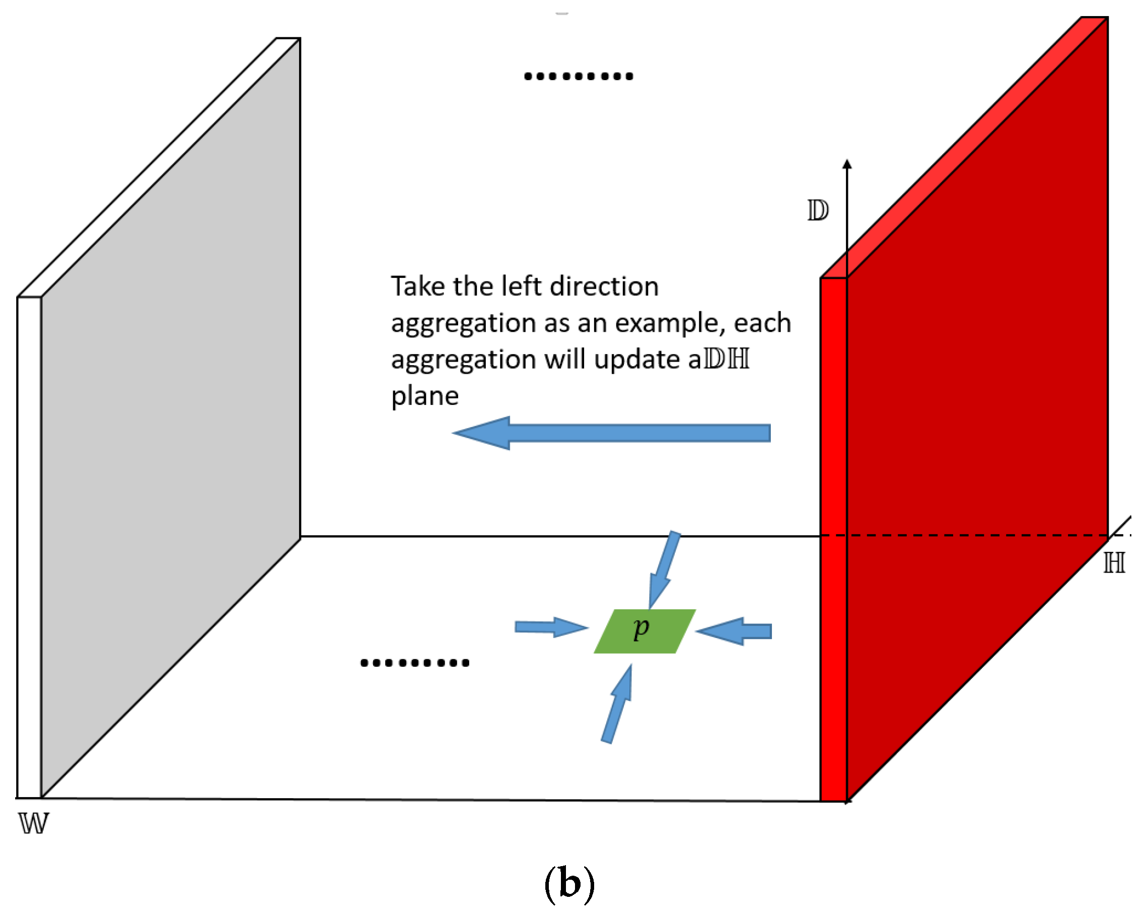
Based on the SGM method, we select four directions (up, down, left, and right) for cost aggregation as shown in Figure 8b. Take the left horizontal direction cost aggregation as an example, the cumulative cost iteration can be expressed as,
where is the position of the cost cube, and are the predefined penalty parameters, represents the matching cost obtained directly from the convolution network, and is the cost after aggregation whose initial value is the output of the neural network, represents the minimum cost of the position in the cost cube for all possible disparity . After the aggregation, one plane will be updated. Similarly, for the up and down directions, the corresponding plane will be updated. Finally, the aggregate values of the four directions are added as the final DSI.
After the above steps, we still choose the disparity according to the principle of minimum cost value. To further improve the accuracy of the disparity map with low complexity, we adopt the inner check method [19] in the left/right consistency check step. The inner check method is to calculate the DSI of the right image through the DSI of the left image rather than network again. Let denote the DSI of the left image, denote the DSI of the right image, denote the disparity map obtained by , and denotes the disparity map obtained by If , pixel is valid in the , otherwise we will mark it as an invalid pixel and assign it with disparity values from surrounding pixels.
4. Experimental Results and Analyses
We used KITTI2015, KITTI2012 binocular dataset to verify the performance of the proposed neural network. The resolution of the images in the dataset is 1242 × 375. We first cropped each image into patches with size of 37 × 37 (for the left image) and 37 × 237 (for the right image). We randomly selected 75% of the images for training, while the remaining images were used for the test. During the training, the batch size is set to be 128. The NVIDIA GeForce GTX 1070Ti graphical card was used for training, and the iteration number was set to be 40000.
4.1. KITTI Datasets Description
The KITTI stereo dataset is filmed by calibrated cameras while driving, such as Figure 10. The content of the dataset mainly includes roads, cities, residential areas, campuses, and pedestrians. The 3D laser scanner can obtain relatively dense distance information, and the depth map of the scene obtained by 3D laser scan can be used as the real disparity map after calculation. The KITTI platform provides 3D point cloud data obtained by 3D scanning lasers, corresponding calibration information, and coordinate transformation information, from which we can generate the real disparity maps.
4.2. Patch Pair Generation
We first cropped the left image into patches with a size of 37 × 37. Then, the ground truth disparity of the central pixel of the patch is recorded. For each of the cropped left image patch, we found the pixel position in the right image according to the ground truth disparity of the pixel . Centered by the position , we cropped the patch with the size of 37 × 237 as the input right image patch, as shown in Figure 3. Then the input of the proposed neural network can be denoted as . Therefore, for the position in the left image patch, there are 200 potential matching positions,
and the aim is of the neural network is to select the optimal matching position. To this end, we also define the label of the neural network to be , as shown in Figure 7.
4.3. Image Sample Processing
In the KITTI2015 dataset, the disparity map is saved in “png” format and the data type is uint16. In the disparity map, the point with a gray value of 0 is an invalid point, that is, there is no real disparity value at this point [12]. For these points, we did not put them into the training set. The disparity map processing is expressed as follows:
where, represents the original disparity map, represents the processed disparity map. The image patch should be further normalized to [0,1] for the input of the proposed neural network.
4.4. Training
We first tested six configurations of layers and convolutional kernels for the proposed neural network without deconvolution layers, as shown in Table 1. 3Conv in the table represents three convolution layers, Conv13 represents 13 × 13 as the size of the convolution kernel in the convolution layer, ReLU represents rectified linear units, BN represents batch normalization function and so forth. By taking the deconvolution layers into the network structure, the overall convolution neural network configurations are given in Table 2, in which 1Deconv(3) stands for a single deconvolution layer with a kernel of 3 × 3.
Moreover, we also verified the effectiveness of the proposed method with different image block input sizes. We try to set the size of the left image block to 29 × 29, 33 × 33, 37 × 37, 41 × 41, and 45 × 45. Accordingly, the right input image block sizes were set to be 29 × 229, 33 × 233, 37 × 237, 41 × 241, 45 × 245.
4.5. Comparison
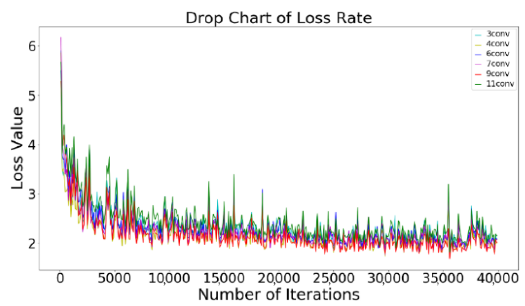
Figure 11 shows the loss curve of each network configuration. We can see that the network with nine convolutional layers and four convolutional layers converges better than the other configurations. Table 3 shows the percentage of missing matching pixels with a threshold of 2, 3, 4, 5 in the test set, in which 37 × 37 represents the size of the input image block. The threshold means the absolute difference between the estimated disparity and the actual disparity. We can see that the network with nine convolutional layers configuration performs better for 2, and 3 pixel errors (with percentages of 10.86% and 8.07%), whereas, the network with four convolution layers configuration performs better for 5 pixels error (with a percentage of 6.01%). For the threshold of 4, the performances are the same as each other. (the percentage is 6.82%).
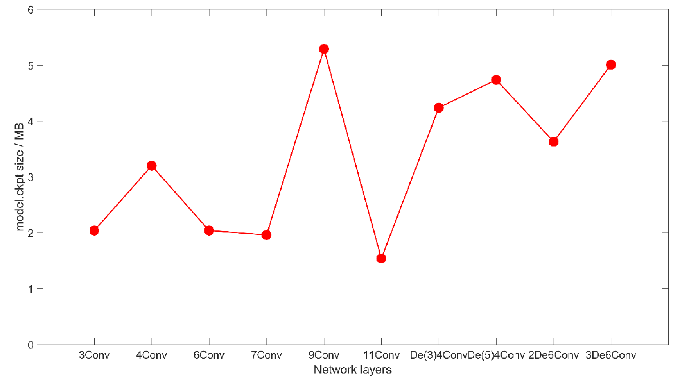
Moreover, Table 4 compares the number of parameters of different network configurations. We can see that the more convolutional layers produce fewer network parameters. In Figure 12, we can see that the network structure that takes up more space of “ckpt” file can obtain better matching results. However, it is difficult to obtain a good matching result if the network parameters are too small such as the network with 11Conv configuration.
Table 5 compares the number of parameters of different network configurations with deconvolution structure. The size of image layers will be increased because of the operation of the deconvolution kernel. Therefore, in the following, the size of the convolution kernels will also be enlarged correspondingly. From Table 4 and Table 5, we can see that the best matching result can be obtained with a constant convolution kernel size and appropriate deconvolution structure layers such as 1Deconv(5) and 4Conv.
Table 6 shows the performances of the neural network with different deconvolution layers. we can see the 1Deconv(5) with 4Conv configuration owns the best performance in the table. The corresponding 2, 3, 4, and 5 pixel errors are only 10.31%, 7.60%, 6.38%, and 5.74%, whereas the errors are 15.02%, 12.99%, 12.04%, and 11.38% for the method in Zbontar [19]. We can also see that excessive usage of deconvolution layers will not always improve the matching accuracy. We believe the reason is that although deconvolution can strengthen the edge information and equip them with better model expression ability, more deconvolution layers will introduce more irrelevant elements such as “0” in formula 6.
As shown in Table 7, we can see that the proposed neural network with deconvolution layers can achieve better matching results in different image block sizes compared to the neural network without deconvolution layers. When the input image block size is 29 × 29, the best result of the neural network without deconvolution layers (4Conv configuration) is 12.76%, 9.98%, 8.63%, 7.84% for the 2, 3, 4, and 5 pixel errors. As a comparison, the best result of the neural network with deconvolution layers (1Deconv(3)-4Conv configuration) is 12.47%, 9.89%, 8.71%, and 8.02%. That is to say, benefiting from the deconvolution layers, better results can be achieved in the cases of 2 and 3 pixel errors. Furthermore, we also enlarged the input image block size to discuss the influence of the block size. When the input image block size is 41 × 41, the best result of the neural network without deconvolution layers (5Conv configuration) is 10.39%, 7.64%, 6.43%, and 5.69% for the 2, 3, 4, and 5 pixel errors, while that with deconvolution layers (also 1Deconv(3)-4Conv configuration) is 9.94%, 7.31%, 6.15%, 5.47%, which are all better than those without deconvolution layers. In summary, equipped with the deconvolution layers, better results can be achieved in most cases, indicating the effectiveness of the proposed method.
To further verify the effectiveness of the proposed neural network, we also undertook the experiments with the KITTI2012 validation set. As shown in Table 8, better results can also be achieved by the proposed neural network. The corresponding 2, 3, 4, and 5 pixels errors are only 8.42%, 7.07%, 6.43%, 6.02%, whereas the errors are 12.86%, 10.64%, 9.65%, and 9.03% for the method in [18].
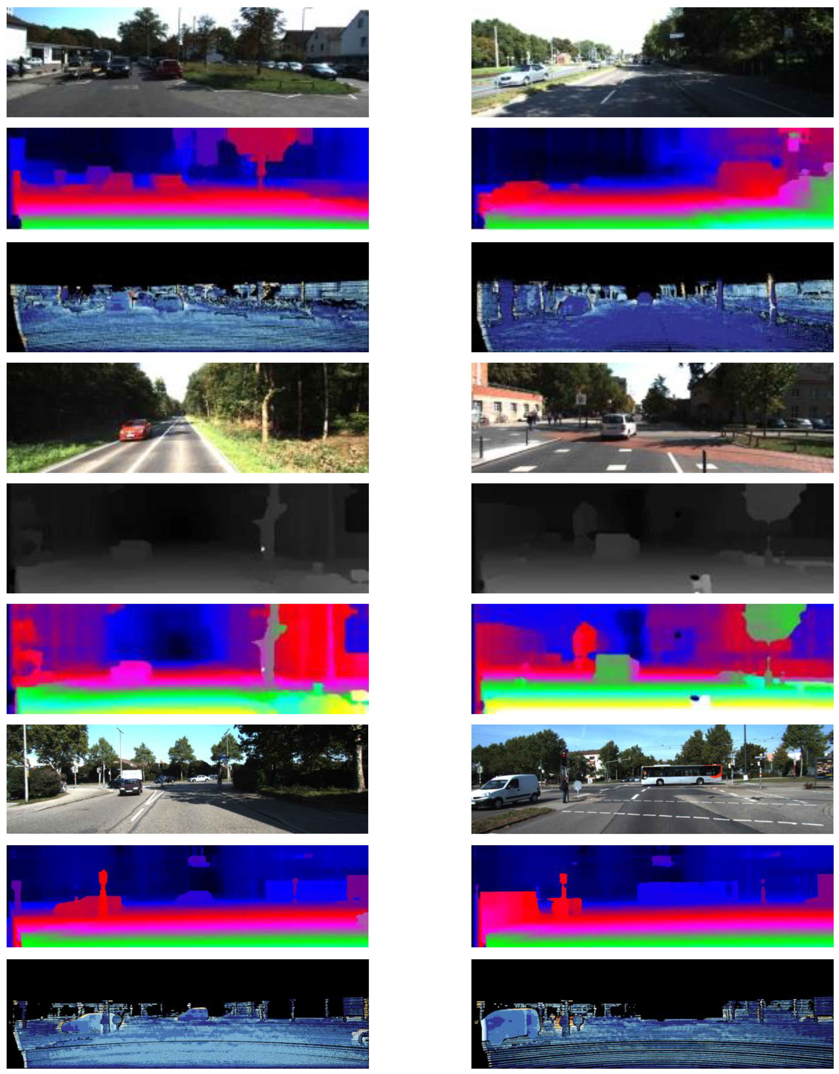
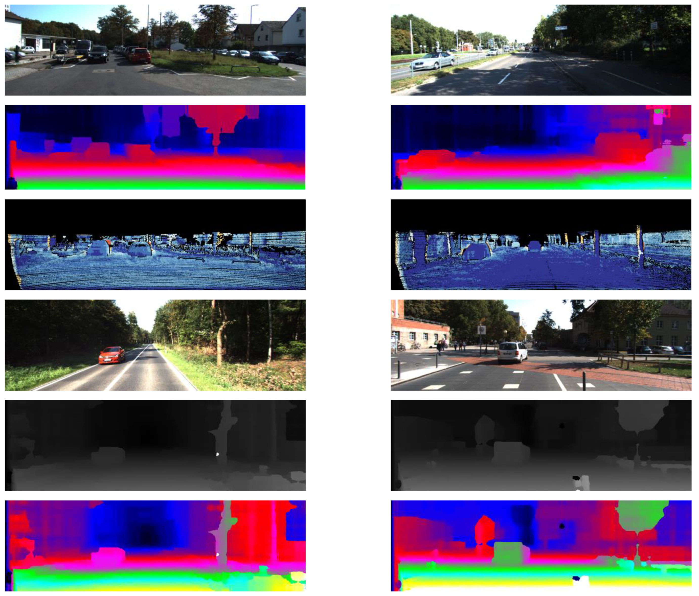
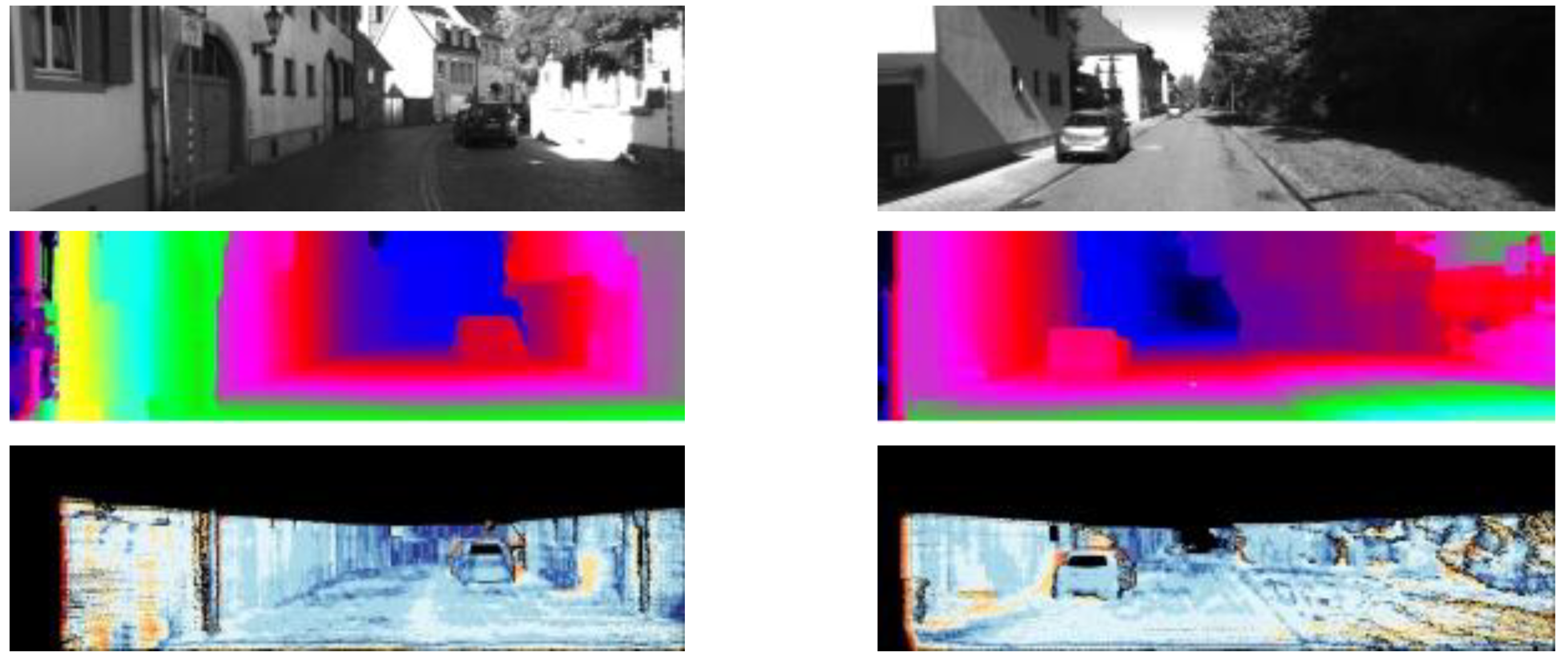
In addition, we also compared the proposed method with the other state-of-the-art methods, MC-CNN [19], Efficient-CNN [18], Elas [28], SGM [20], SPSS [30], PCBP-SS [30], StereoSLIC [31], Displets v2 [32] in Table 9 and Table 10, respectively. From Table 9, we can see that, for the KITTI2012 dataset, the DispletsV2 [32] is the best, the corresponding 2, 3, 4, and 5 pixel errors are 4.46%, 3.09%, 2.52%, and 2.17%. However, we should also note that the accuracy is achieved with great computational complexity. The processing time for a picture on average is 265 s. The MC-CNN-acrt also achieves good results, i.e., the 2, 3, 4, and 5 pixel errors are 5.45%, 3.63%, 2.85%, and 2.39%. However, its processing time is still large, i.e., 67 s. The proposed method can achieve comparable accuracy (i.e., 5.62%, 4.01%, 3.02%, and 2.65% for 2,3,4, and 5 pixel errors) with a much small processing time, i.e., 2.4 s. For the results of the KITTI2015 dataset, as shown in Table 10, we can see that the proposed method can achieve the smallest 2 pixel error (4.27%). The 3, 4, and 5 pixel errors (3.85%, 2.57%, and 2.00%) of the proposed method is only a little larger than MC-CNN-slow which achieves the best accuracy on the whole. However, the processing time of the proposed method is only 2.5 s on average, which is much smaller than MC-CNN-slow. Disparity maps and error maps obtained by final matching are shown in Figure 13 and Figure 14.
5. Conclusions and Future Work
To improve the accuracy of stereo matching, based on CNN stereo matching, we designed a novel neural network structure by adding a deconvolution operation before the formal convolutional layers. The deconvolution operation introduced at the beginning of the network increases the size of the input features maps for the following convolution layers, and as a result the whole convolution network learns more information. Besides, we also dropped the fully connected layer and replaced it with a dot product to enable it to obtain matching results in a short time. Experimental results demonstrated that better matching results can be achieved by the proposed neural network structure (with the configuration of 37-1Deconv(5) and 4Conv) with low inference and training time complexity.
Author Contributions
Conceptualization, X.M. and Z.Z.; methodology, X.M. and Z.Z.; software, D.W. and Z.Z.; validation, Y.L. and H.Y.; formal analysis, H.Y.; investigation, Y.L.; resources, Y.L.; data curation, Z.Z.; writing—original draft preparation, X.M. and Z.Z.; writing—review and editing, X.M. and Z.Z.; visualization, Z.Z.; supervision, Y.L.; project administration, Y.L.; funding acquisition, Y.L. All authors have read and agreed to the published version of the manuscript.
Funding
This work was funded by the Shandong Natural Science Foundation (Grants No. ZR2021MF114) and in part by the National Natural Science Foundation of China under Grants 61871342.
Institutional Review Board Statement
Not applicable.
Informed Consent Statement
Not applicable.
Data Availability Statement
The data set website and the paper link are as follows: http://www.cvlibs.net/datasets/kitti/raw_data.php (accessed on 8 January 2022).
Acknowledgments
The authors would like to thank the editors and anonymous reviewers for their valuable comments.
Conflicts of Interest
The authors declare no conflict of interest.
References
- Li, T.; Liu, C.; Liu, Y.; Wang, T.; Yang, D. Binocular stereo vision calibration based on alternate adjustment algorithm. Opt. Int. J. Light Electron. Opt. 2018, 173, 13–20. [Google Scholar] [CrossRef]
- Weber, J.W.; Atkin, M. Further results on the use of binocular vision for highway driving. In Proceedings of the SPIE; The International Society for Optical Engineering, Bellingham, WA, USA; 1997; Volume 2902. [Google Scholar]
- Nalpantidis, L.; Sirakoulis, G.C.; Gasteratos, A. Review of stereo matching algorithms for 3D vision. In Proceedings of the International Symposium on Measurement & Control in Robotics, Warsaw, Poland, 21–23 June 2007. [Google Scholar]
- Zhang, K.; Lu, J.; Lafruit, G. Cross-Based Local Stereo Matching Using Orthogonal Integral Images. IEEE Trans. Circuits Syst. Video Technol. 2009, 19, 1073–1079. [Google Scholar] [CrossRef]
- Jiao, J.; Wang, R.; Wang, W.; Dong, S.; Wang, Z.; Gao, W. Local Stereo Matching with Improved Matching Cost and Disparity Refinement. IEEE MultiMedia 2014, 21, 16–27. [Google Scholar] [CrossRef]
- Deng, Y.; Yang, Q.; Lin, X.; Tang, X. Stereo Correspondence with Occlusion Handling in a Symmetric Patch-Based Graph-Cuts Model. IEEE Trans. Pattern Anal. Mach. Intell. 2007, 29, 1068–1079. [Google Scholar] [CrossRef] [PubMed] [Green Version]
- Zhang, X.; Dai, H.; Sun, H.; Zheng, N. Algorithm and VLSI Architecture Co-Design on Efficient Semi-Global Stereo Matching. IEEE Trans. Circuits Syst. Video Technol. 2019, 30, 4390–4403. [Google Scholar] [CrossRef]
- Hsiao, S.-F.; Wang, W.-L.; Wu, P.-S. VLSI implementations of stereo matching using Dynamic Programming. In Proceedings of the Technical Papers of 2014 International Symposium on VLSI Design, Automation and Test, Hsinchu, Taiwan, 28–30 April 2014; pp. 1–4. [Google Scholar] [CrossRef]
- Xiang, X.; Zhang, M.; Li, G.; He, Y.; Pan, Z. Real-time stereo matching based on fast belief propagation. Mach. Vis. Appl. 2012, 23, 1219–1227. [Google Scholar] [CrossRef]
- Wang, X.; Wang, H.; Su, Y. Accurate Belief Propagation with parametric and non-parametric measure for stereo matching. Opt. Int. J. Light Electron. Opt. 2015, 126, 545–550. [Google Scholar] [CrossRef]
- Papadakis, N.; Caselles, V. Multi-label depth estimation for graph cuts stereo problems. J. Math. Imaging Vis. 2010, 38, 70–82. [Google Scholar] [CrossRef]
- Gao, H.; Chen, L.; Liu, X.; Yu, Y. Research of an improved dense matching algorithm based on graph cuts. In Proceedings of the 2010 8th World Congress on Intelligent Control and Automation, Jinan, China, 7–9 July 2010; pp. 6053–6057. [Google Scholar] [CrossRef]
- Zagoruyko, S.; Komodakis, N. Learning to compare image patches via convolutional neural networks. In Proceedings of the IEEE Conference on Computer Vision and Pattern Recognition, Boston, MA, USA, 7–12 June 2015; pp. 4353–4361. [Google Scholar]
- Seki, A.; Pollefeys, M. Patch based confidence prediction for dense disparity map. In Proceedings of the British Machine Vision Conference (BMVC), York, UK, 19–22 September 2016; Volume 2, p. 4. [Google Scholar]
- Chang, J.-R.; Chen, Y.-S. Pyramid stereo matching network. In Proceedings of the IEEE Conference on Computer Vision and Pattern Recognition, Salt Lake City, UT, USA, 18–23 June 2018. [Google Scholar]
- Zbontar, J.; LeCun, Y. Computing the stereo matching cost with a convolutional neural network. In Proceedings of the IEEE Conference on Computer Vision and Pattern Recognition, Boston, MA, USA, 7–12 June 2015. [Google Scholar]
- Liu, X.; Luo, Y.; Ye, Y.; Lu, J. Dilated convolutional neural network for computing stereo matching cost. In International Conference on Neural Information Processing; Springer: Cham, Switzerland, 2017. [Google Scholar]
- Luo, W.; Schwing, A.G.; Urtasun, R. Efficient deep learning for stereo matching. In Proceedings of the IEEE Conference on Computer Vision and Pattern Recognition, Las Vegas, NV, USA, 27–30 June 2016. [Google Scholar]
- Zbontar, J.; LeCun, Y. Stereo matching by training a convolutional neural network to compare image patches. J. Mach. Learn. Res. 2006, 17, 2287–2318. [Google Scholar]
- Hirschmuller, H. Stereo Processing by Semiglobal Matching and Mutual Information. IEEE Trans. Pattern Anal. Mach. Intell. 2008, 30, 328–341. [Google Scholar] [CrossRef] [PubMed]
- Gundewar, P.P.; Abhyankar, H.K. Analysis of region based stereo matching algorithms. In Proceedings of the 2014 Annual IEEE India Conference (INDICON), Pune, India, 11–13 December 2014. [Google Scholar]
- He, K.; Sun, J.; Tang, X. Guided image filtering. In European Conference on Computer Vision; Springer: Berlin/Heidelberg, Germany, 2010. [Google Scholar]
- Mayer, N.; Ilg, E.; Hausser, P.; Fischer, P.; Cremers, D.; Dosovitskiy, A.; Brox, T. A large dataset to train convolutional networks for disparity, optical flow, and scene flow estimation. In Proceedings of the IEEE Conference on Computer Vision and Pattern Recognition (CVPR), Las Vegas, NV, USA, 27–30 June 2016; pp. 4040–4048. [Google Scholar]
- Pang, J.; Sun, W.; Ren, J.S.; Yang, C.; Yan, Q. Cascade residual learning: A two-stage convolutional neural network for stereo matching. In Proceedings of the IEEE International Conference on Computer Vision Workshops (ICCVW), Venice, Italy, 22–29 October 2017. [Google Scholar]
- Khamis, S.; Fanello, S.; Rhemann, C.; Kowdle, A.; Valentin, J.; Izadi, S. StereoNet: Guided Hierarchical Refinement for Real-Time Edge-Aware Depth Prediction. In Proceedings of the European Conference on Computer Vision, Munich, Germany, 8–14 September 2018; pp. 596–613. [Google Scholar]
- Feng, Y.; Liang, Z.; Liu, H. Efficient deep learning for stereo matching with larger image patches. In Proceedings of the 2017 10th International Congress on Image and Signal Processing, BioMedical Engineering and Informatics (CISP-BMEI), Shanghai, China, 14–16 October 2017. [Google Scholar]
- Geiger, A.; Roser, M.; Urtasun, R. EfficientLarge-ScaleStereo Matching. In Asian Conference on Computer Vision; Springer: Berlin/Heidelberg, Germany, 2010. [Google Scholar]
- Zeiler, M.D.; Krishnan, D.; Taylor, G.W.; Fergus, R. Deconvolutional networks. In Proceedings of the 2010 IEEE Computer Society Conference on Computer Vision and Pattern Recognition, San Francisco, CA, USA, 13–18 June 2010. [Google Scholar]
- Melekhov, I.; Kannala, J.; Rahtu, E. Siamese network features for image matching. In Proceedings of the 2016 23rd International Conference on Pattern Recognition (ICPR), Cancun, Mexico, 4–8 December 2016. [Google Scholar]
- Yamaguchi, K.; McAllester, D.; Urtasun, R. Efficient Joint Segmentation, Occlusion Labeling, Stereo and Flow Estimation. In European Conference on Computer Vision; Springer: Cham, Switzerland, 2014. [Google Scholar]
- Yamaguchi, K.; McAllester, D.; Urtasun, R. Robust Monocular Epipolar Flow Estimation. In Proceedings of the 2013 IEEE Conference on Computer Vision and Pattern Recognition, Portland, OR, USA, 23–28 June 2013; pp. 1862–1869. [Google Scholar] [CrossRef] [Green Version]
- Guney, F.; Geiger, A. Displets: Resolving stereo ambiguities using object knowledge. In Proceedings of the 2015 IEEE Conference on Computer Vision and Pattern Recognition (CVPR), Boston, MA, USA, 7–12 June 2015; pp. 4165–4175. [Google Scholar] [CrossRef]
Figure 1.
Binocular vision camera model converts binocular vision into a coordinate system.

Figure 2.
Adaptive deconvolution-based disparity matching net (ADSM) network structure. This structure only consists of a convolutional layer and deconvolution layer. At the end, it compares the label with dot product produced by the extracted features.
Figure 2.
Adaptive deconvolution-based disparity matching net (ADSM) network structure. This structure only consists of a convolutional layer and deconvolution layer. At the end, it compares the label with dot product produced by the extracted features.

Figure 3.
The overall structure of the stereo matching algorithm. The left and right image will pass through ASDM Net and generate a three-dimensional array called the DSI (disparity space image). After four-way cost aggregation, a new DSI will be generated. In this paper, we will use the quadratic fitting method to directly attend the sub-pixel level. After that, we use the inner check method to check the left and right consistency and finally, use the ray filling method to fill the invalid pixel position.

Figure 4.
Illustration of the input left and right image patches. Since the input images have been rectified by pole line, the center of the left and right image are all on the uniform line.
Figure 4.
Illustration of the input left and right image patches. Since the input images have been rectified by pole line, the center of the left and right image are all on the uniform line.

Figure 5.
The operation of the one-step of deconvolution. Deconvolution is similar to convolution except that it can enlarge the original image.
Figure 5.
The operation of the one-step of deconvolution. Deconvolution is similar to convolution except that it can enlarge the original image.

Figure 6.
Illustration of convolution and deconvolution. (a,b) represent the convolution operation, the green part represents the convolution result and blue part represents the input, the shadow part represents the size of convolution kernel. (c,d) represent the deconvolution operation, the green part represents the deconvolution result, the blue part represents the input and the shadow part represents the kernel of deconvolution.

Figure 7.
(a,b) represent different weight values for calculating cross entropy loss.

Figure 8.
Disparity space image-based aggregation illustration, (a) represents disparity space image, (b) represents aggregation along with the left horizontal direction.
Figure 8.
Disparity space image-based aggregation illustration, (a) represents disparity space image, (b) represents aggregation along with the left horizontal direction.


Figure 9.
The upper image was generated by the proposed neural network with 4Conv, the following image was generated by 1Deconv(5) and 4Conv. The input block size was set to be 37 × 37.
Figure 9.
The upper image was generated by the proposed neural network with 4Conv, the following image was generated by 1Deconv(5) and 4Conv. The input block size was set to be 37 × 37.

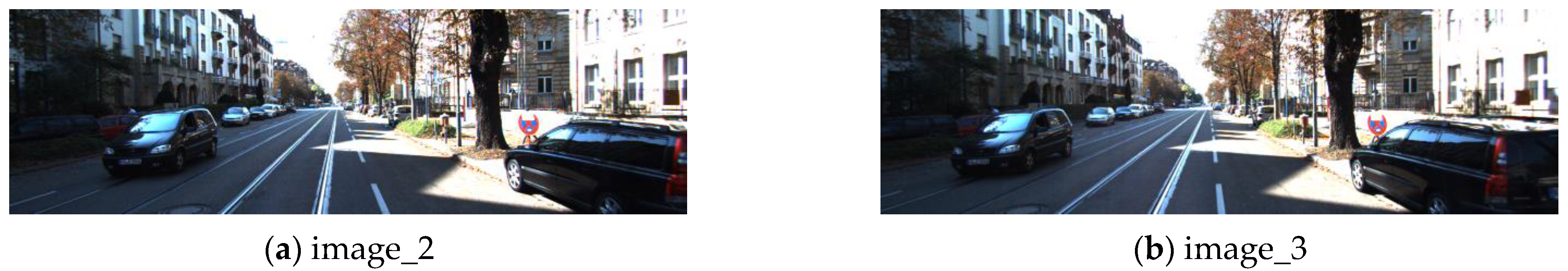
Figure 10.
Sample images of KITTI2015 dataset.

Figure 11.
Loss curve of different network configurations.

Figure 12.
The network model (model.ckpt file) size after training for different network structures. The ckpt file is a binary file from tensoflow, which stores all the weights, bias, gradients and other variables.
Figure 12.
The network model (model.ckpt file) size after training for different network structures. The ckpt file is a binary file from tensoflow, which stores all the weights, bias, gradients and other variables.

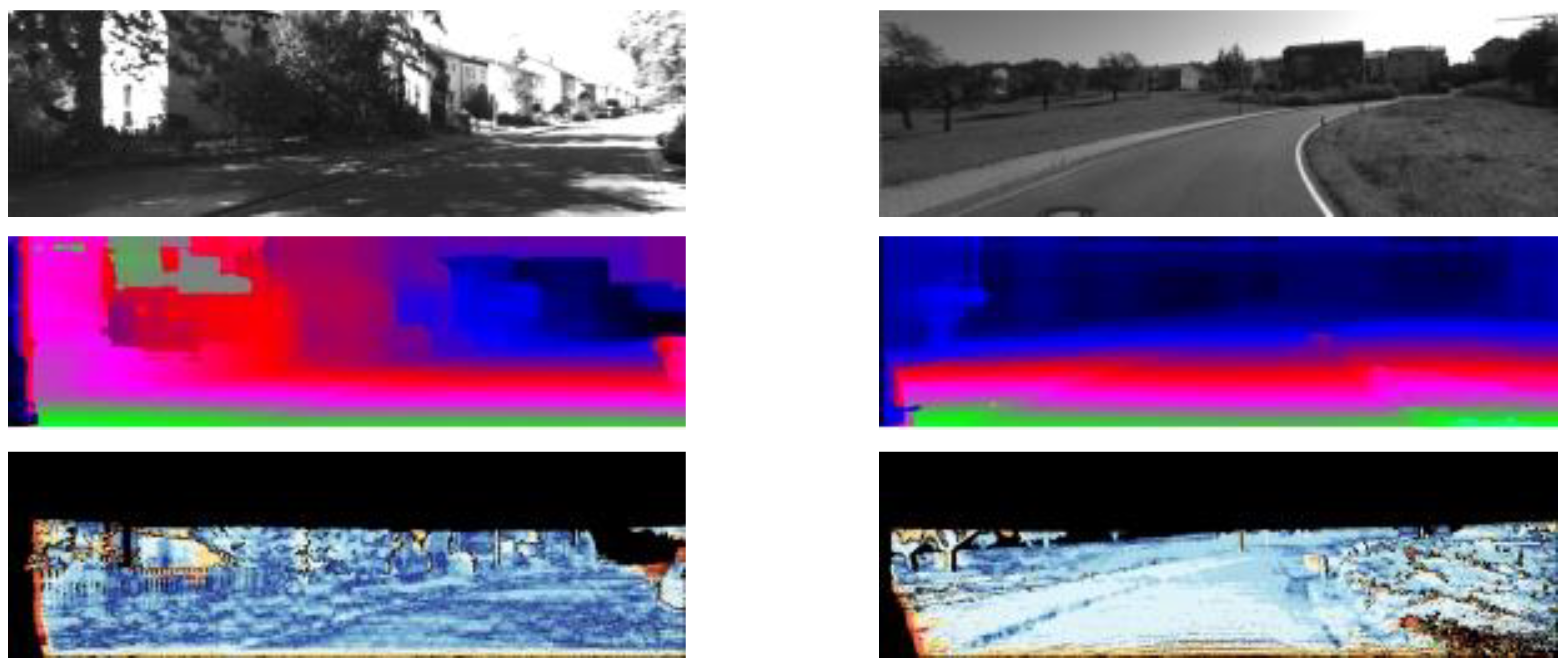
Figure 13.
KITTI2015 test set: (top) original image, (center) stereo estimates, (bottom) stereo errors.
Figure 13.
KITTI2015 test set: (top) original image, (center) stereo estimates, (bottom) stereo errors.


Figure 14.
KITTI2012 test set: (top) original image, (center) stereo estimates, (bottom) stereo errors.
Figure 14.
KITTI2012 test set: (top) original image, (center) stereo estimates, (bottom) stereo errors.


Table 1.
Six configurations of convolutional layers for the proposed neural network.
| 3Conv | 4Conv | 6Conv |
|---|---|---|
| Conv13 + BN + ReLU | Conv10 + BN + ReLU | Conv9 + BN + ReLU |
| Conv13 + BN + ReLU | Conv10 + BN + ReLU | Conv9 + BN + ReLU |
| Conv13 + softmax | Conv10 + BN + ReLU | Conv7 + BN + ReLU |
| Conv10 + softmax | Conv7 + BN + ReLU | |
| Conv5 + BN + ReLU | ||
| Conv5 + softmax | ||
| 7Conv | 9Conv | 11Conv |
| Conv7 + BN + ReLU | Conv5 + BN + ReLU | Conv5 + BN + ReLU |
| Conv7 + BN + ReLU | Conv5 + BN + ReLU | Conv5 + BN + ReLU |
| Conv7 + BN + ReLU | Conv5 + BN + ReLU | Conv5 + BN + ReLU |
| Conv7 + BN + ReLU | Conv5 + BN + ReLU | Conv5 + BN + ReLU |
| Conv5 + BN + ReLU | Conv5 + BN + ReLU | Conv5 + BN + ReLU |
| Conv5 + BN + ReLU | Conv5 + BN + ReLU | Conv5 + BN + ReLU |
| Conv5 + softmax | Conv5 + BN + ReLU | Conv5 + BN + ReLU |
| Conv5 + BN + ReLU | Conv3 + BN + ReLU | |
| Conv5 + softmax | Conv3 + BN + ReLU | |
| Conv3 + BN + ReLU | ||
| Conv3 + softmax |
Table 2.
The overall convolution neural network configurations for the proposed neural network.
| 1Deconv(5) and 4Conv | 1Deconv(3) and 4Conv | 2Deconv and 6Conv | 3Deconv and 6Conv |
|---|---|---|---|
| Deconv5 + BN | Deconv3 + BN | Deconv3 + BN | Deconv3 + BN + ReLU |
| Conv11 + BN + ReLU | Conv11 + BN + ReLU | Deconv5 + BN | Deconv5 + BN + ReLU |
| Conv11 + BN + ReLU | Conv11 + BN + ReLU | Conv9 + BN + ReLU | Deconv7 + BN + ReLU |
| Conv11 + BN + ReLU | Conv10 + BN + ReLU | Conv9 + BN + ReLU | Conv9 + BN + ReLU |
| Conv11 + softmax | Conv10 + softmax | Conv9 + BN + ReLU | Conv9 + BN + ReLU |
| Conv7 + BN + ReLU | Conv9 + BN + ReLU | ||
| Conv7 + BN + ReLU | Conv7 + BN + ReLU | ||
| Conv7 + softmax | Conv7 + BN + ReLU | ||
| Conv7 + softmax |
Table 3.
The percentage of missing matching pixels with threshold of 2, 3, 4, 5 in the 2015 KITTI test set.
Table 3.
The percentage of missing matching pixels with threshold of 2, 3, 4, 5 in the 2015 KITTI test set.
| ConvNet-ValError | 2-Pixel-Error | 3-Pixel-Error | 4-Pixel-Error | 5-Pixel-Error |
|---|---|---|---|---|
| 37-3Conv | 12.21 | 8.55 | 6.95 | 6.05 |
| 37-4Conv | 11.11 | 8.12 | 6.82 | 6.01 |
| 37-6Conv | 11.79 | 8.73 | 8.35 | 6.53 |
| 37-7Conv | 11.96 | 8.87 | 7.53 | 6.73 |
| 37-9Conv | 10.86 | 8.07 | 6.82 | 6.07 |
| 37-11Conv | 14.95 | 10.36 | 8.82 | 7.92 |
Table 4.
The number of network parameters of different network structures for input left patch size 37.
Table 4.
The number of network parameters of different network structures for input left patch size 37.
| NetworkType | 3Conv | 4Conv | 6Conv | 7Conv | 9Conv | 11Conv |
|---|---|---|---|---|---|---|
| Number of unilateral network parameters | 1,416,896 | 1,248,000 | 953,536 | 918,720 | 721,600 | 627,932 |
Table 5.
The number of network parameters with deconvolution structure for input left patch size 37.
Table 5.
The number of network parameters with deconvolution structure for input left patch size 37.
| Network Type | 1Deconv(5) and 4Conv | 1Deconv(3) and 4Conv | 2Deconv and 6Conv | 3Deconv and 6Conv |
|---|---|---|---|---|
| Number of unilateral network parameters | 1,987,264 | 1,812,160 | 1,701,568 | 1,902,182 |
Table 6.
The results with deconvolution structure and other network for input left patch size 37.
| ConvNet-ValError | 2-Pixel-Error | 3-Pixel-Error | 4-Pixel-Error | 5-Pixel-Error |
|---|---|---|---|---|
| 37-1Deconv(5) and 4Conv | 10.31 | 7.60 | 6.38 | 5.74 |
| 37-1Deconv(3) and 4Conv | 10.36 | 7.67 | 6.49 | 5.78 |
| 37-2Deconv and 6Conv | 13.63 | 10.56 | 9.27 | 8.53 |
| 37-3Deconv and 6Conv | 15.65 | 12.46 | 11.17 | 10.45 |
| MC-CNN-acrt [19] | 15.02 | 12.99 | 12.04 | 11.38 |
| MC-CNN-fast [19] | 18.47 | 14.96 | 13.18 | 12.02 |
| Efficient-Net [18] | 11.67 | 8.97 | 7.62 | 6.78 |
Table 7.
The percentage of missing matching pixels with threshold of 2, 3, 4, 5 in the 2015 KITTI test set for input left patch size 29, 33, 41, 45.
Table 7.
The percentage of missing matching pixels with threshold of 2, 3, 4, 5 in the 2015 KITTI test set for input left patch size 29, 33, 41, 45.
| Input Patch Size | ConvNetModel | 2-Pixel-Error | 3-Pixel-Error | 4-Pixel-Error | 5-Pixel-Error |
|---|---|---|---|---|---|
| 3Conv | 13.49 | 10.29 | 8.79 | 7.92 | |
| 4Conv | 12.76 | 9.98 | 8.63 | 7.84 | |
| 5Conv | 12.8 | 10.1 | 8.78 | 8.03 | |
| 29 × 29 | 7Conv | 13.21 | 10.44 | 9.13 | 8.36 |
| 1Deconv(3)-4Conv | 12.47 | 9.89 | 8.71 | 8.02 | |
| 1Deconv(2)-4Conv | 12.96 | 10.28 | 9.04 | 8.32 | |
| 4Conv | 12.34 | 9.59 | 8.25 | 7.45 | |
| 8Conv | 13.11 | 10.31 | 8.63 | 7.84 | |
| 33 × 33 | 1Deconv(3)-4Conv | 12.20 | 9.70 | 8.55 | 7.88 |
| 1Deconv(5)-4Conv | 12.80 | 10.20 | 9.03 | 8.35 | |
| 4Conv | 10.61 | 7.69 | 6.41 | 5.66 | |
| 5Conv | 10.39 | 7.64 | 6.43 | 5.69 | |
| 8Conv | 11.03 | 8.21 | 6.96 | 6.21 | |
| 41 × 41 | 10Conv | 11.47 | 8.51 | 7.21 | 6.45 |
| 1Deconv(3)-4Conv | 9.94 | 7.31 | 6.15 | 5.47 | |
| 1Deconv(5)-4Conv | 10.26 | 7.51 | 6.29 | 5.56 | |
| 4Conv | 10.48 | 7.55 | 6.24 | 5.47 | |
| 45 × 45 | 5Conv | 10.54 | 7.69 | 6.44 | 5.69 |
| 8Conv | 10.78 | 7.88 | 6.62 | 5.85 | |
| 1Deconv(3)-4Conv | 9.45 | 6.86 | 5.72 | 5.03 |
Table 8.
The percentage of missing matching pixels with thresholds of 2, 3, 4, 5 in the 2012 KITTI validation set.
Table 8.
The percentage of missing matching pixels with thresholds of 2, 3, 4, 5 in the 2012 KITTI validation set.
| ConvNetModel | 2-Pixel-Error | 3-Pixel-Error | 4-Pixel-Error | 5-Pixel-Error |
|---|---|---|---|---|
| MC-CNN-acrt [21] | 16.92 | 14.93 | 13.98 | 13.32 |
| MC-CNN-fast [21] | 19.56 | 17.41 | 16.31 | 15.51 |
| Efficient-Net [15] | 12.86 | 10.64 | 9.65 | 9.03 |
| Ours | 8.42 | 7.07 | 6.43 | 6.02 |
Table 9.
Error comparison of disparity with different algorithms (KITTI2012) %.
| Algorithm | 2-Pixel-Error | 3-Pixel-Error | 4-Pixel-Error | 5-Pixel-Error | Runtime (s) |
|---|---|---|---|---|---|
| StereoSLIC [31] | 7.20 | 5.11 | 4.04 | 3.33 | 2.3 |
| PCBP-SS [30] | 6.75 | 4.72 | 3.75 | 3.15 | 300 |
| SPSS [30] | 6.28 | 4.41 | 3.52 | 3.00 | 2 |
| MC-CNN-acrt [19] | 5.45 | 3.63 | 2.85 | 2.39 | 67 |
| Displets v2 [32] | 4.46 | 3.09 | 2.52 | 2.17 | 265 |
| Efficient-CNN [18] | 6.51 | 4.29 | 3.36 | 2.82 | 0.7 |
| Ours | 5.62 | 4.01 | 3.02 | 2.65 | 2.4 |
Table 10.
Error comparison of disparity with different algorithms (KITTI2015) %.
| Algorithm | 2-Pixel-Error | 3-Pixel-Error | 4-Pixel-Error | 5-Pixel-Error | Runtime (s) |
|---|---|---|---|---|---|
| Elas [28] | 24.09 | 19.21 | 17.59 | 16.82 | 0.669 |
| SGM [20] | 10.03 | 6.93 | 5.47 | 4.48 | 1.8 |
| SPSS [30] | 7.15 | 4.58 | 3.46 | 2.93 | 3 |
| Efficient-CNN [18] | 6.78 | 4.38 | 2.56 | 2.03 | 1 |
| MC-CNN-fast [19] | 7.53 | 4.01 | 2.84 | 2.33 | 0.2 |
| MC-CNN-slow [19] | 6.38 | 3.27 | 2.37 | 1.97 | 35 |
| Ours | 4.27 | 3.85 | 2.57 | 2.00 | 2.5 |
Publisher’s Note: MDPI stays neutral with regard to jurisdictional claims in published maps and institutional affiliations. |
© 2022 by the authors. Licensee MDPI, Basel, Switzerland. This article is an open access article distributed under the terms and conditions of the Creative Commons Attribution (CC BY) license (https://creativecommons.org/licenses/by/4.0/).
Share and Cite
MDPI and ACS Style
Ma, X.; Zhang, Z.; Wang, D.; Luo, Y.; Yuan, H. Adaptive Deconvolution-Based Stereo Matching Net for Local Stereo Matching. Appl. Sci. 2022, 12, 2086. https://0-doi-org.brum.beds.ac.uk/10.3390/app12042086
AMA Style
Ma X, Zhang Z, Wang D, Luo Y, Yuan H. Adaptive Deconvolution-Based Stereo Matching Net for Local Stereo Matching. Applied Sciences. 2022; 12(4):2086. https://0-doi-org.brum.beds.ac.uk/10.3390/app12042086
Chicago/Turabian StyleMa, Xin, Zhicheng Zhang, Danfeng Wang, Yu Luo, and Hui Yuan. 2022. "Adaptive Deconvolution-Based Stereo Matching Net for Local Stereo Matching" Applied Sciences 12, no. 4: 2086. https://0-doi-org.brum.beds.ac.uk/10.3390/app12042086
Note that from the first issue of 2016, this journal uses article numbers instead of page numbers. See further details here.