
Prediction of Pile Bearing Capacity Using XGBoost Algorithm: Modeling and Performance Evaluation

 , ,
, ,  and
and
Abstract
:1. Introduction
- To develop a model that is able to learn the complex relationship among axial pile bearing capacity and its influencing factors with reasonable precision.
- To validate the proposed model by comparing the efficacy with prominent modeling techniques, such as AdaBoost, RF, DT, and SVM in terms of performance measure metrics.
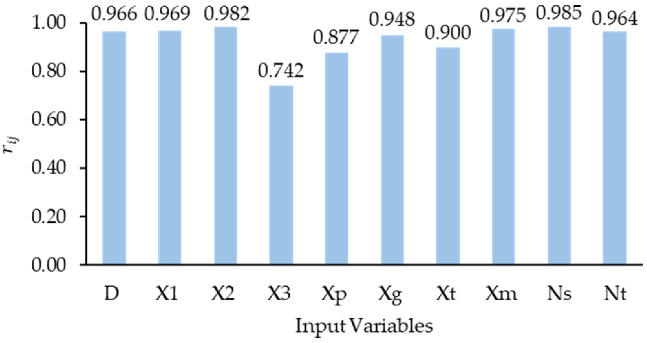
- To conduct sensitivity analyses for the determination of the effect of each input parameter on Pu.
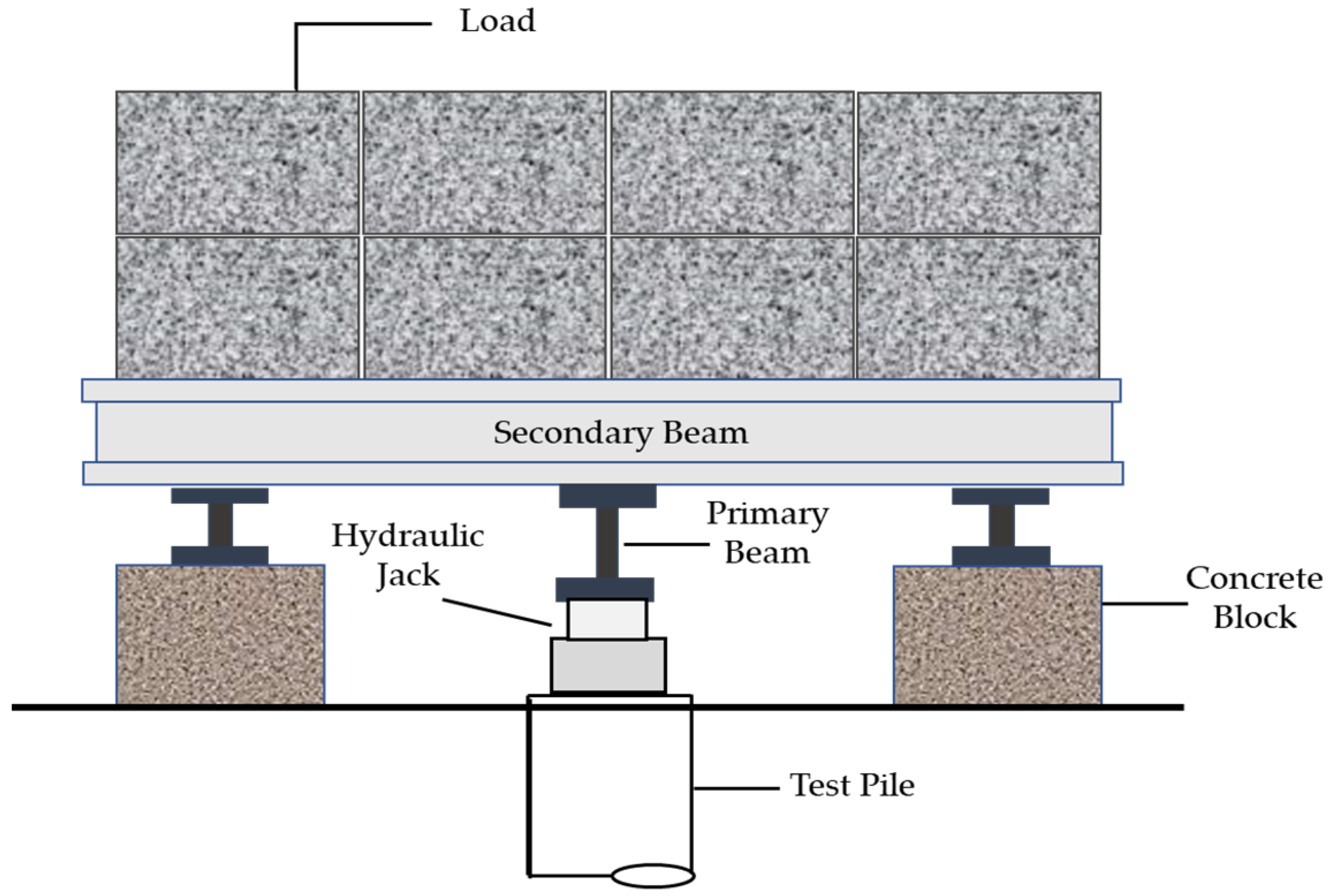
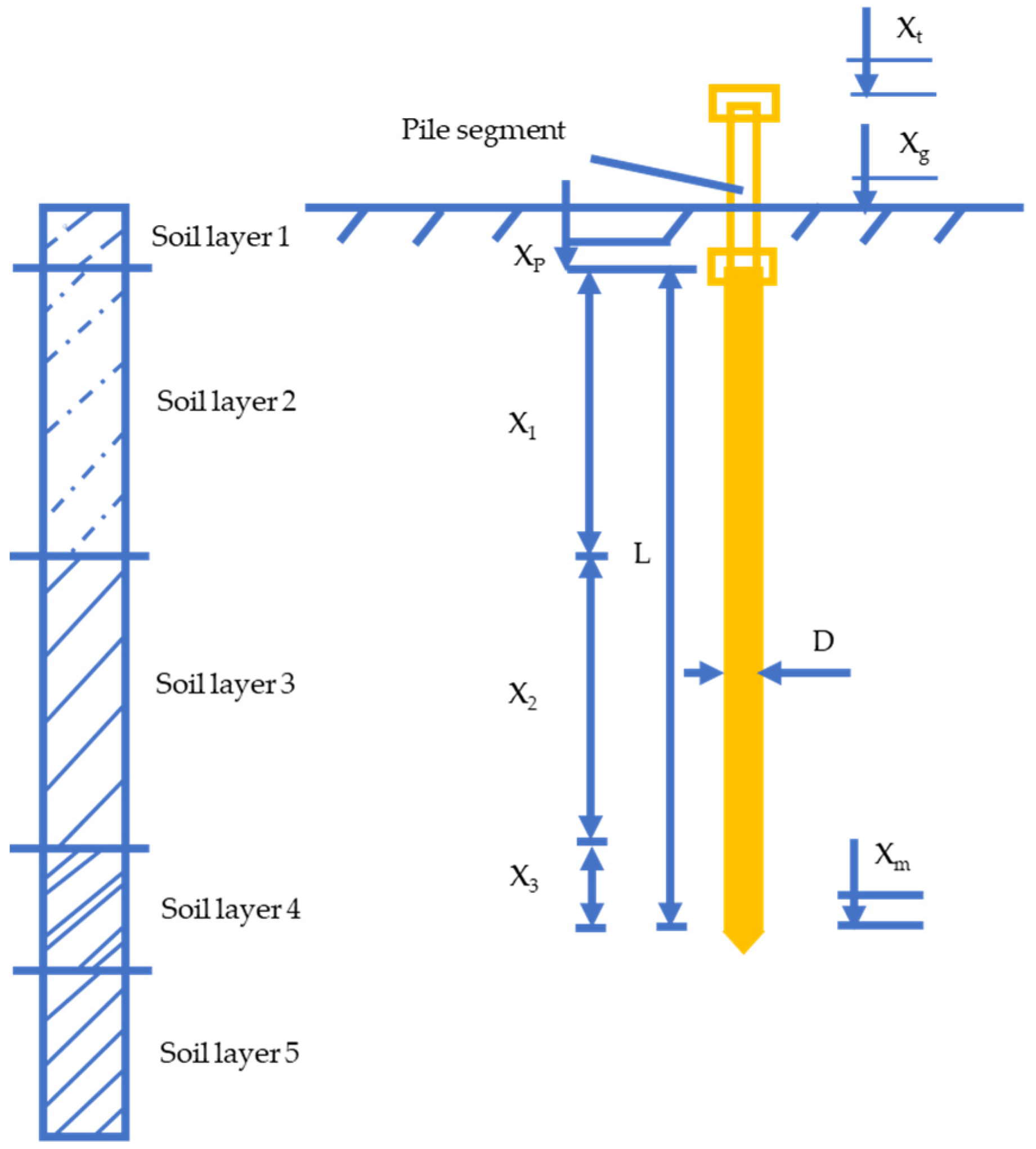
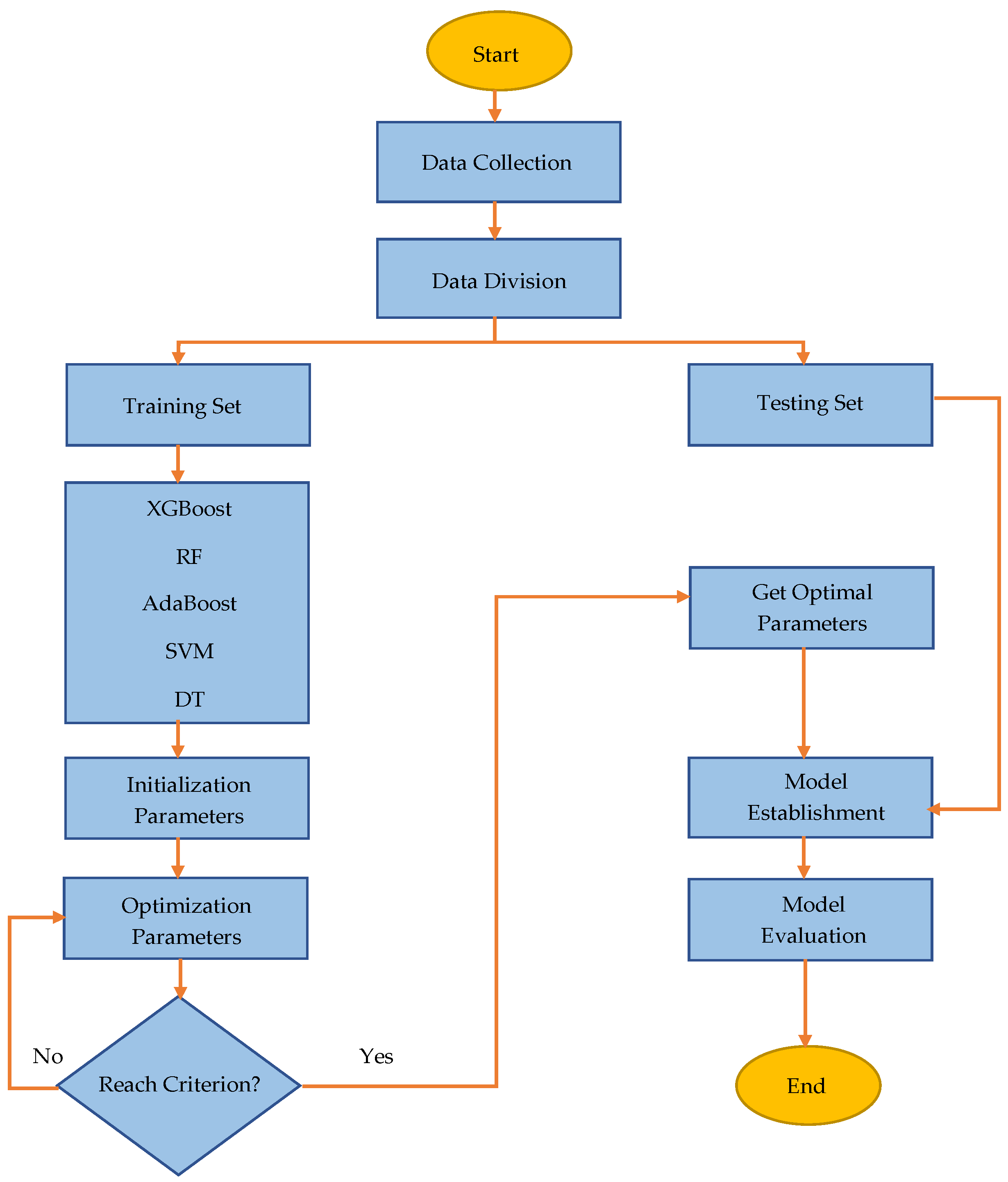
2. Data Collection and Preparation
2.1. Dataset
- (i)
- the pile bearing capacity was taken as the failure load when the settlement of pile top at the current load level was five times or higher than the settlement of pile top at the previous load level;
- (ii)
- when the load–settlement curve became linear at the last test load, condition (i) would not be used. In such a case, the test load at which progressive movement occurs or the total settlement exceeds 10 % of the pile diameter or width would be taken as the pile bearing capacity.
2.2. Correlation Analysis
3. Machine Learning Methods
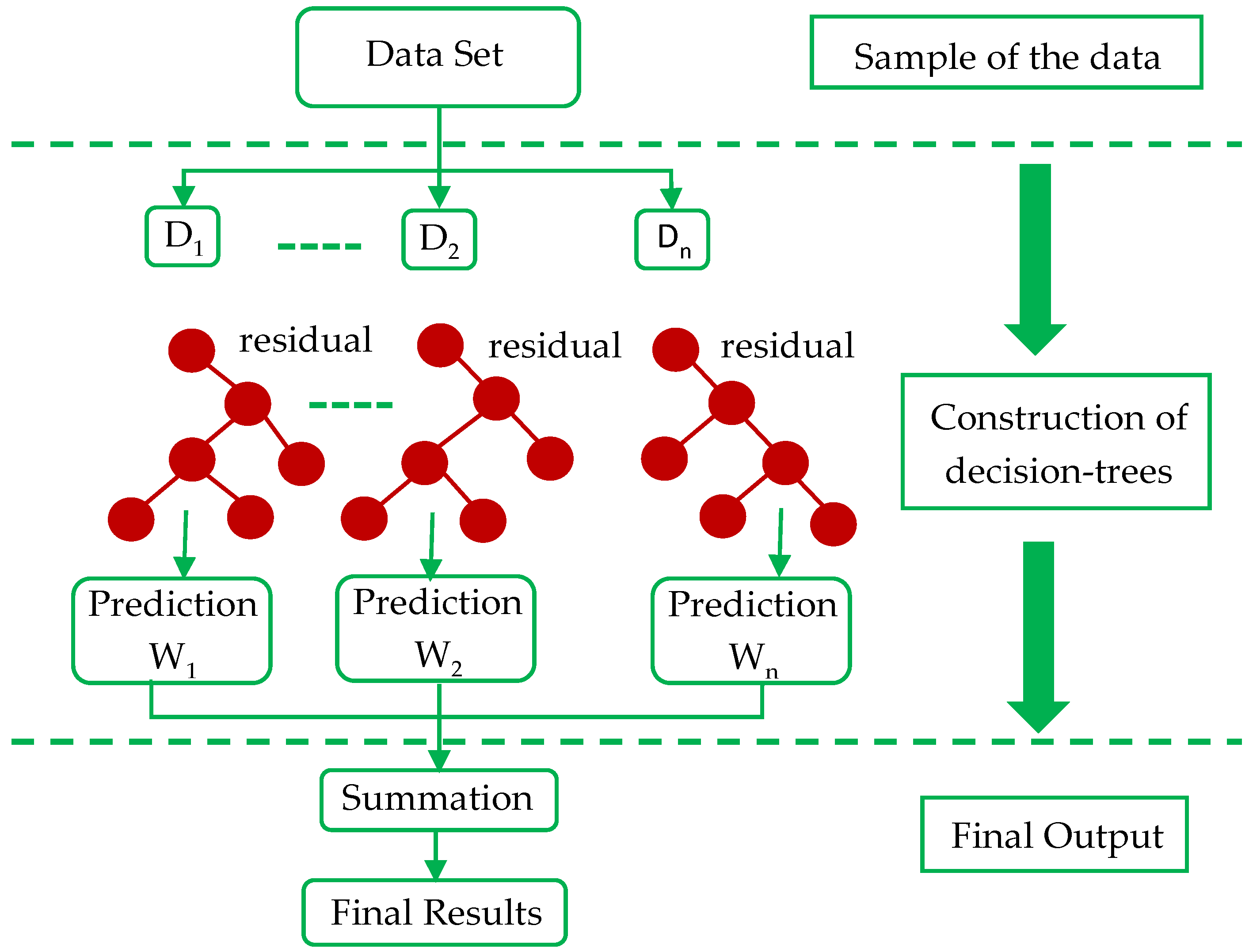
3.1. Extreme Gradient Boosting Algorithm
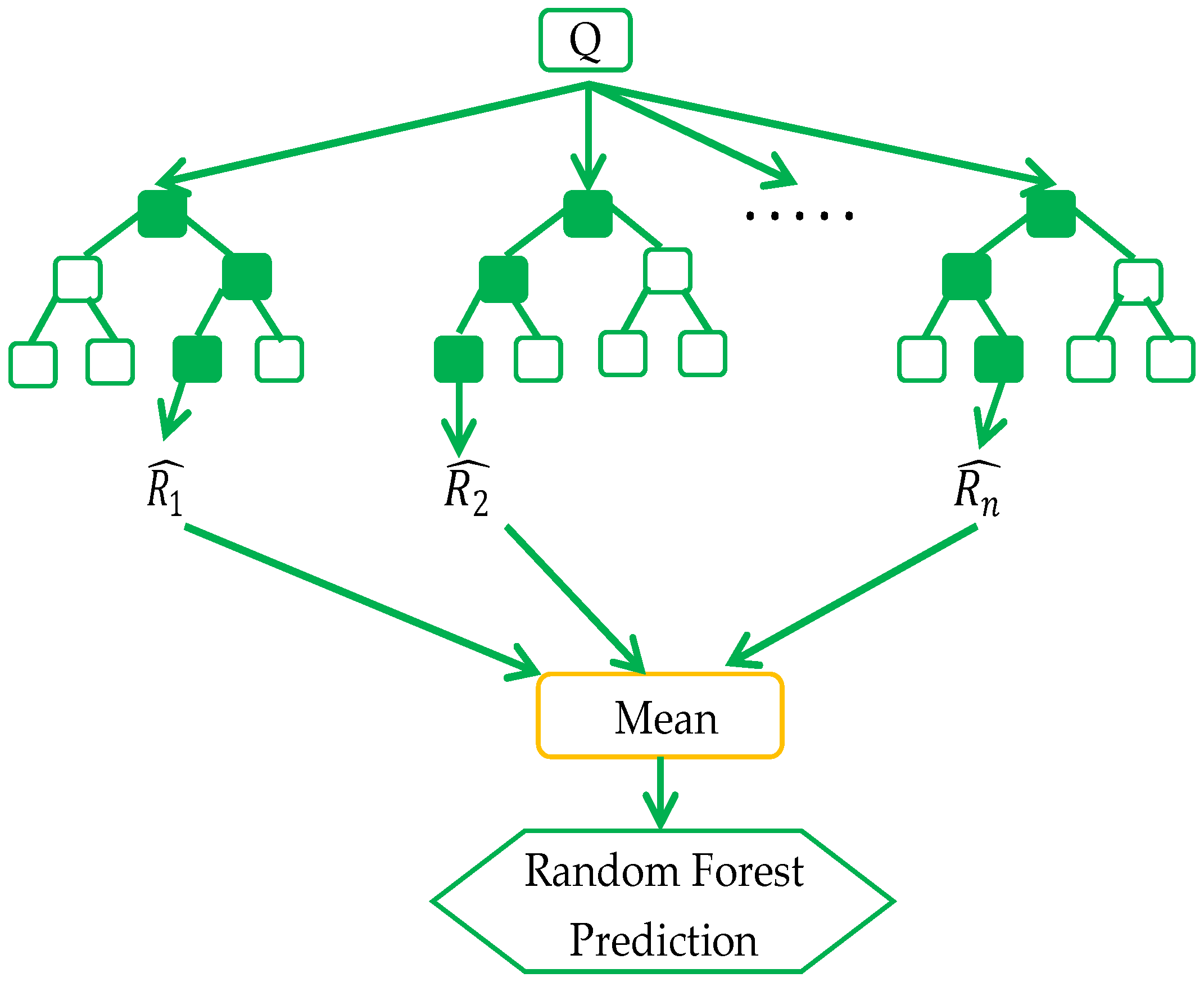
3.2. Random Forest (RF) Algorithm
3.3. AdaBoost Algorithm
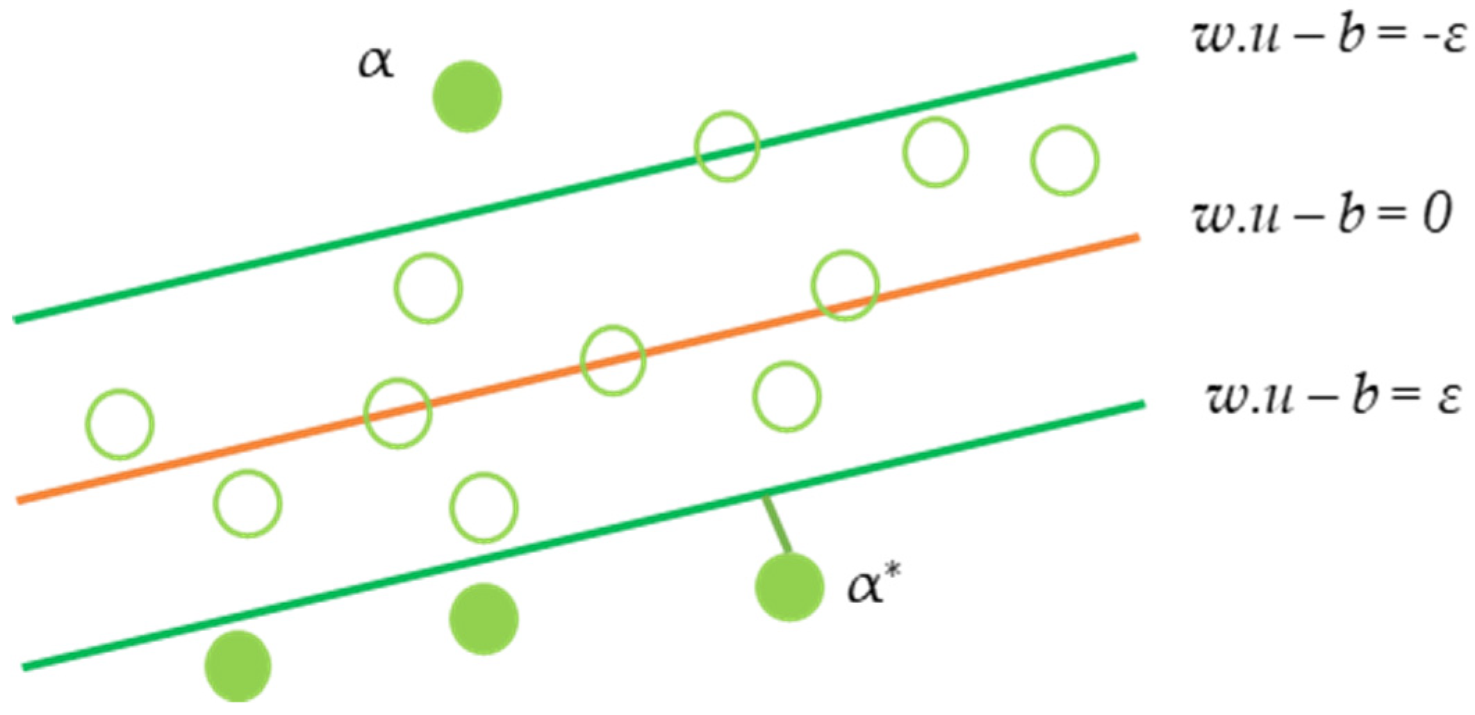
3.4. Support Vector Machine (SVM) Algorithm
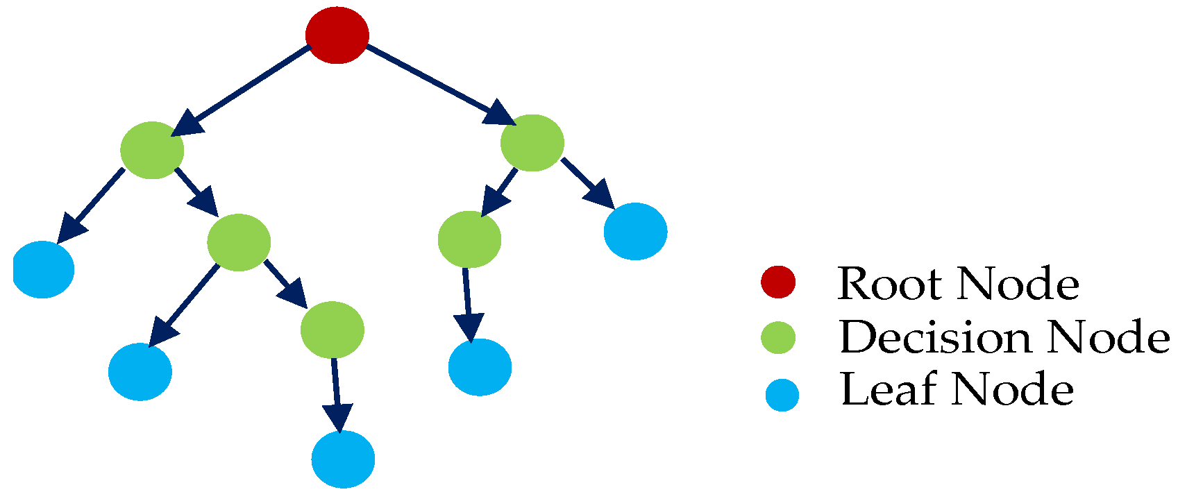
3.5. Decision Tree (DT) Algorithm
4. Construction of Prediction Models
4.1. Hyperparameter Optimization
4.2. Model Evaluation Indexes
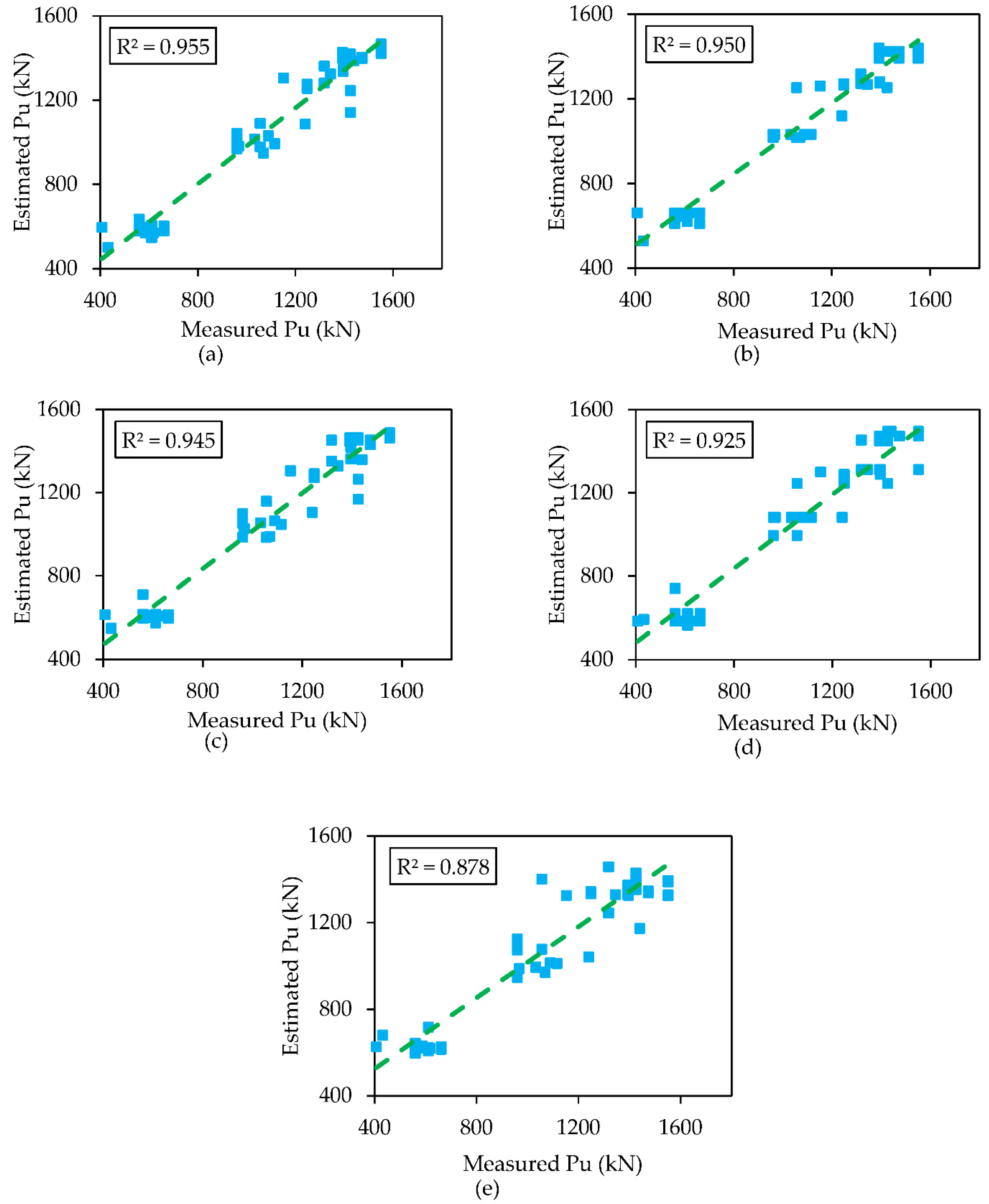
5. Result and Discussion
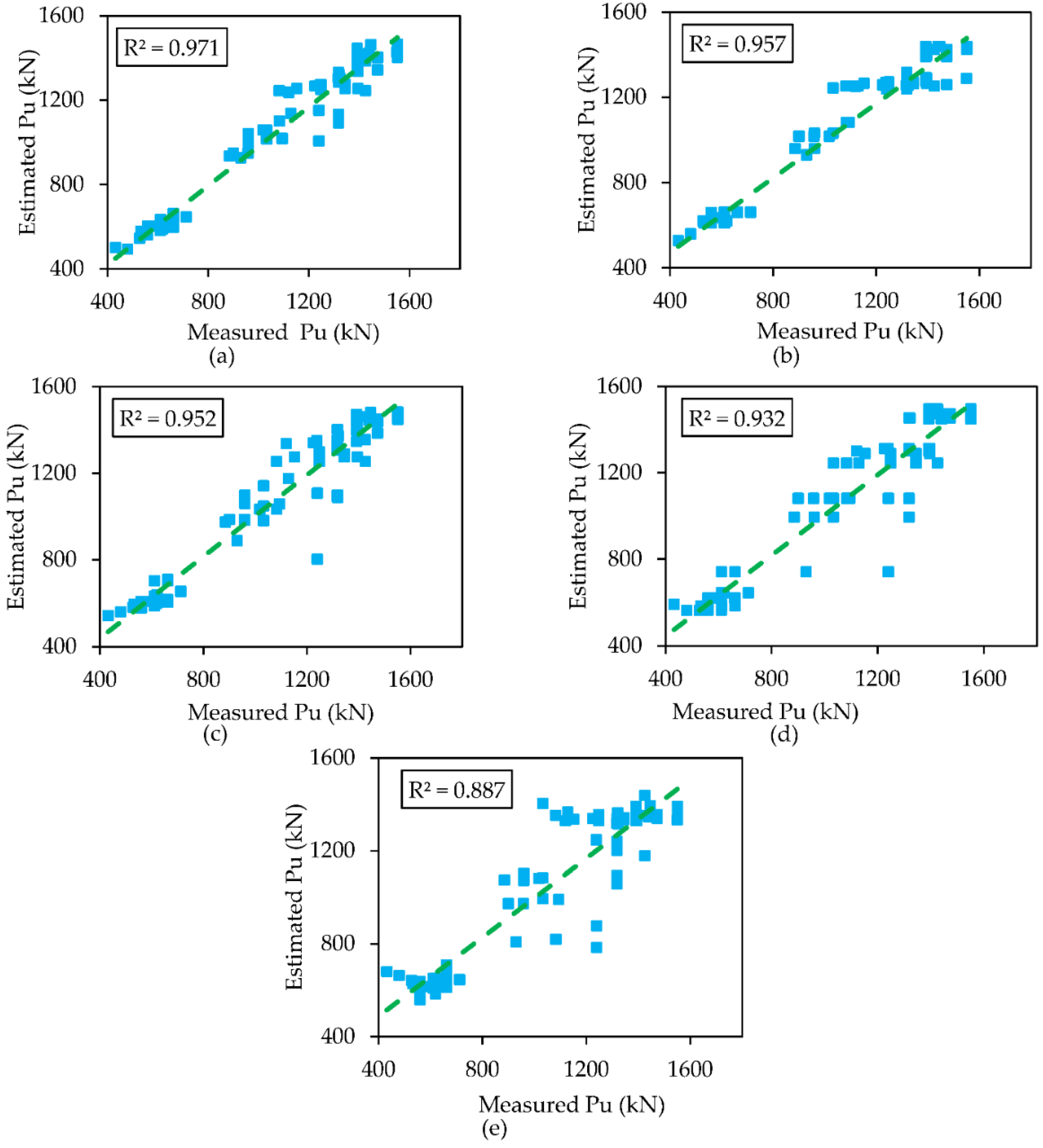
5.1. Comparison of Models
5.2. Comparison with Other Researchers
6. Conclusions
- In testing phase, the XGBoost model (R2 = 0.955, MAE = 59.929, RMSE = 80.653, MARE = 6.6, NSE = 0.950, and RSR = 0.225) has the highest performance capability as compared to other soft computing techniques considered in this study i.e., AdaBoost, RF, DT and SVM as well as the models used in the literature.
- Sensitivity analysis results show that SPT blow count at pile shaft (NS) was the most important parameter in predicting pile bearing capacity.
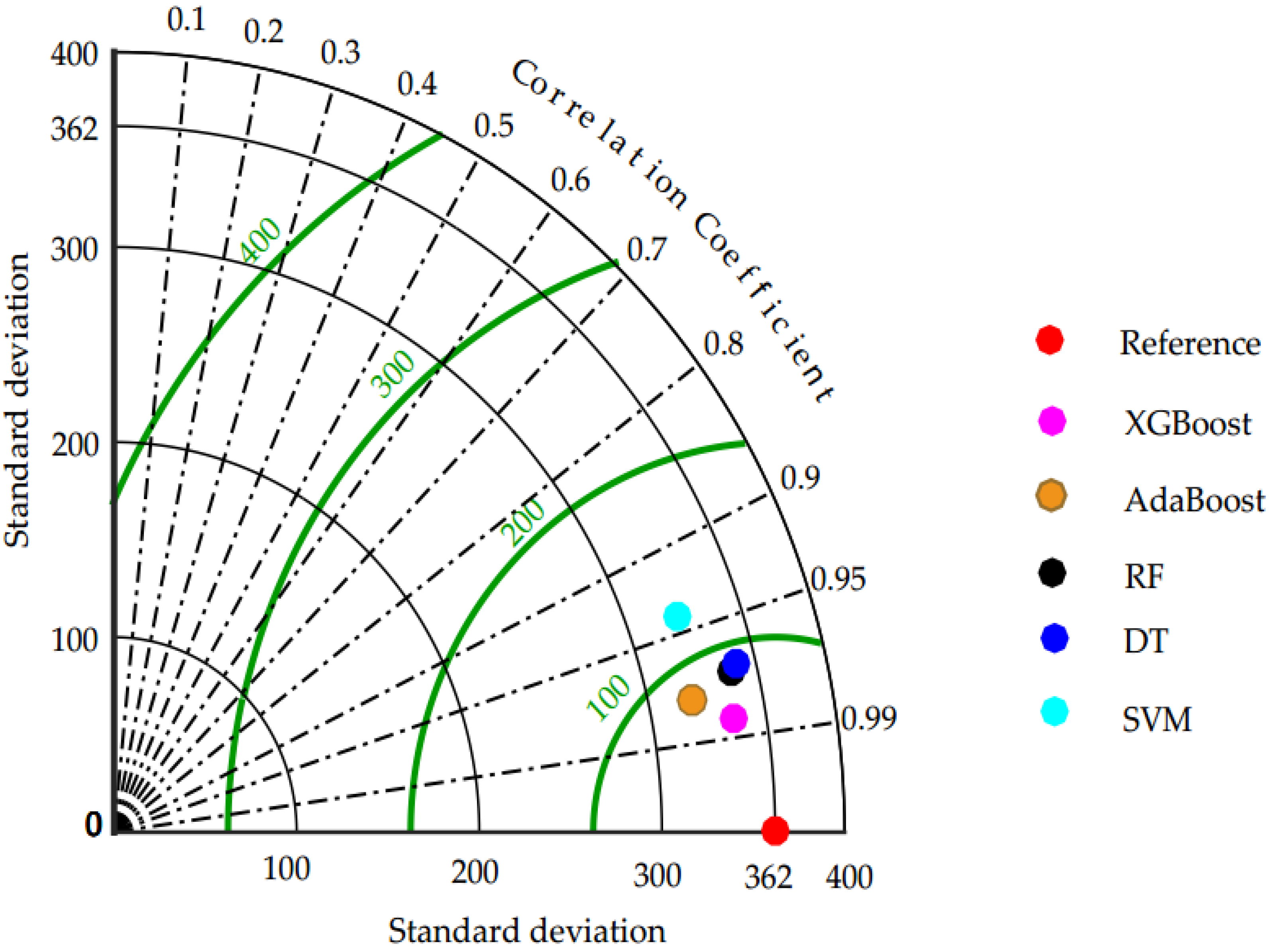
- Taylor diagram also verified that all the models are good but the predictive power of the XGBoost algorithm had a higher correlation and lower RMSE.
- Based on the results and analysis the XGBoost model can also be applied to solve a variety of geotechnical engineering problems.
Author Contributions
Funding
Institutional Review Board Statement
Informed Consent Statement
Data Availability Statement
Acknowledgments
Conflicts of Interest
Abbreviation
| Symbol | Explanation |
| Pu | Pile bearing capacity |
| ML | Machine learning |
| XGBoost | Extreme gradient boosting |
| AdaBoost | Adaptive boosting |
| RF | Random forest |
| DT | Decision tree |
| SVM | Support vector machine |
| ANN | Artificial neural network |
| ANFIS | adaptive neuro-fuzzy inference system |
| GA | Genetic algorithm |
| BPNN | Backpropagation neural network |
| GBDT | Gradient boosting decision tree |
| LightGBM | Light gradient boosting machine |
| DLNN | Deep Learning Neural Network |
| PSO-ANN | Particle swarm optimization—ANN |
| GPR | Gaussian process regression |
| R2 | Coefficient of determination |
| MAE | Mean absolute error |
| MSE | Mean square error |
| RMSE | Root mean square error |
| MARE | Mean absolute relative error |
| NSE | Nash–Sutcliffe model efficiency |
| RSR | Relative strength ratio |
| SPT | Standard penetration test |
| CPT | Cone penetration test |
| D | Diameter |
| X1 | Depth of first layer of soil embedded |
| X2 | Depth of second layer of soil embedded |
| X3 | Depth of third layer of soil embedded |
| Xp | Pile top elevation |
| Xg | Ground elevation |
| Xt | Extra pile top elevation |
| Xm | Pile tip elevation |
| NS | SPT blow count at pile shaft |
| Nt | SPT blow count at pile tip |
Appendix A

| S. No. | D | X1 | X2 | X3 | Xp | Xg | Xt | Xm | Ns | Nt | Pu |
|---|---|---|---|---|---|---|---|---|---|---|---|
| Unit | mm | m | m | m | m | m | m | m | - | - | kN |
| 1 | 400 | 3.45 | 8 | 0.3 | 2.95 | 3.65 | 2.95 | 14.7 | 11.75 | 7.59 | 1017.9 |
| 2 | 400 | 4.25 | 8 | 1 | 2.15 | 3.56 | 2.16 | 15.4 | 13.25 | 7.67 | 1152 |
| 3 | 400 | 4.25 | 8 | 1.02 | 2.15 | 3.58 | 2.16 | 15.42 | 13.27 | 7.68 | 1344 |
| 4 | 400 | 4.25 | 8 | 0.1 | 2.15 | 3.58 | 3.08 | 14.5 | 12.35 | 7.14 | 1551 |
| 5 | 400 | 4.35 | 8 | 1.06 | 2.05 | 3.55 | 2.09 | 15.46 | 13.41 | 7.66 | 1321 |
| 6 | 300 | 3.4 | 5.25 | 0 | 3.4 | 3.49 | 3.44 | 12.05 | 8.65 | 6.75 | 559.8 |
| 7 | 400 | 4.25 | 8 | 1.02 | 2.15 | 3.58 | 2.16 | 15.42 | 13.27 | 7.68 | 1248 |
| 8 | 300 | 3.4 | 5.18 | 0 | 3.4 | 3.36 | 3.38 | 11.98 | 8.58 | 6.73 | 559.8 |
| 9 | 400 | 4.75 | 7.25 | 0 | 2.05 | 3.62 | 3.57 | 14.05 | 12 | 6.73 | 1425 |
| 10 | 300 | 3.4 | 5.25 | 0 | 3.4 | 3.47 | 3.42 | 12.05 | 8.65 | 6.75 | 559.8 |
| 11 | 300 | 3.4 | 5.2 | 0 | 3.4 | 3.42 | 3.42 | 12 | 8.6 | 6.73 | 660.6 |
| 12 | 400 | 3.45 | 5.24 | 0 | 3.35 | 3.44 | 3.4 | 12.04 | 8.69 | 6.72 | 1240 |
| 13 | 400 | 4.35 | 8 | 1.07 | 2.05 | 3.52 | 2.05 | 15.47 | 13.42 | 7.67 | 1425 |
| 14 | 400 | 4.1 | 2.17 | 0 | 2.7 | 3.7 | 2.73 | 8.97 | 6.27 | 4.92 | 661.6 |
| 15 | 400 | 3.55 | 5.39 | 0 | 3.25 | 3.44 | 3.25 | 12.19 | 8.94 | 6.72 | 1083 |
| 16 | 400 | 4.25 | 8 | 1 | 2.15 | 3.56 | 2.16 | 15.4 | 13.25 | 7.67 | 1152 |
| 17 | 400 | 3.4 | 7.3 | 0 | 3.4 | 3.61 | 3.51 | 14.1 | 10.7 | 7.28 | 1115.2 |
| 18 | 300 | 3.4 | 5.2 | 0 | 3.4 | 3.43 | 3.43 | 12 | 8.6 | 6.73 | 610.7 |
| 19 | 300 | 3.4 | 5.2 | 0 | 3.4 | 3.42 | 3.42 | 12 | 8.6 | 6.73 | 661.6 |
| 20 | 400 | 4.1 | 1.8 | 0 | 2.7 | 3.39 | 2.79 | 8.6 | 5.9 | 4.64 | 620 |
| 21 | 400 | 3.45 | 8 | 0.3 | 2.95 | 3.66 | 2.96 | 14.7 | 11.75 | 7.59 | 960 |
| 22 | 300 | 3.4 | 5.27 | 0 | 3.4 | 3.49 | 3.42 | 12.07 | 8.67 | 6.75 | 559.8 |
| 23 | 400 | 4.25 | 8 | 1 | 2.15 | 3.56 | 2.16 | 15.4 | 13.25 | 7.67 | 1248 |
| 24 | 400 | 4.65 | 7.4 | 0 | 2.15 | 3.59 | 3.39 | 14.2 | 12.05 | 6.80 | 1551 |
| 25 | 400 | 4.1 | 2 | 0 | 2.7 | 3.56 | 2.76 | 8.8 | 6.1 | 4.80 | 620 |
| 26 | 400 | 4.35 | 8 | 0.3 | 2.05 | 3.45 | 2.75 | 14.7 | 12.65 | 7.22 | 1473 |
| 27 | 400 | 4.35 | 8 | 1.03 | 2.05 | 3.48 | 2.05 | 15.43 | 13.38 | 7.65 | 1318 |
| 28 | 400 | 4.35 | 8 | 1.01 | 2.05 | 3.46 | 2.05 | 15.41 | 13.36 | 7.64 | 1473 |
| 29 | 400 | 4.1 | 1.72 | 0 | 2.7 | 3.27 | 2.75 | 8.52 | 5.82 | 4.57 | 423.9 |
| 30 | 400 | 3.4 | 7.28 | 0 | 3.4 | 3.48 | 3.4 | 14.08 | 10.68 | 7.27 | 1318 |
| 31 | 400 | 4.35 | 8 | 1.05 | 2.05 | 3.55 | 2.1 | 15.45 | 13.4 | 7.66 | 1221.5 |
| 32 | 300 | 3.4 | 5.2 | 0 | 3.4 | 3.43 | 3.43 | 12 | 8.6 | 6.73 | 559.8 |
| 33 | 400 | 4.25 | 8 | 0.96 | 2.15 | 3.53 | 2.17 | 15.36 | 13.21 | 7.65 | 1344 |
| 34 | 400 | 4.65 | 7.35 | 0 | 2.15 | 3.55 | 3.4 | 14.15 | 12 | 6.79 | 1392 |
| 35 | 400 | 3.85 | 7.5 | 0 | 2.95 | 3.68 | 3.38 | 14.3 | 11.35 | 7.13 | 1425 |
| 36 | 300 | 3.4 | 5.35 | 0 | 3.4 | 3.57 | 3.42 | 12.15 | 8.75 | 6.78 | 661.6 |
| 37 | 400 | 4.75 | 7.5 | 0 | 2.05 | 3.6 | 3.3 | 14.3 | 12.25 | 6.79 | 1425 |
| 38 | 400 | 4.35 | 8 | 0.95 | 2.05 | 3.41 | 2.06 | 15.35 | 13.3 | 7.60 | 1323.2 |
| 39 | 400 | 4.25 | 8 | 0.9 | 2.15 | 3.57 | 2.27 | 15.3 | 13.15 | 7.61 | 1473 |
| 40 | 400 | 4.35 | 8 | 0.96 | 2.05 | 3.42 | 2.06 | 15.36 | 13.31 | 7.61 | 1244 |
| 41 | 400 | 4.35 | 8 | 1.05 | 2.05 | 3.5 | 4.35 | 15.45 | 13.4 | 7.66 | 1297.8 |
| 42 | 400 | 4.65 | 7.4 | 0 | 2.15 | 3.59 | 3.39 | 14.2 | 12.05 | 6.80 | 1551 |
| 43 | 400 | 4.65 | 7.2 | 0 | 2.15 | 3.58 | 3.58 | 14 | 11.85 | 6.75 | 1551 |
| 44 | 400 | 4.1 | 2 | 0 | 2.7 | 3.5 | 2.7 | 8.8 | 6.1 | 4.80 | 610.7 |
| 45 | 400 | 4.35 | 8 | 0.95 | 2.05 | 3.44 | 2.09 | 15.35 | 13.3 | 7.60 | 1152 |
| 46 | 400 | 4.05 | 8 | 0.66 | 2.35 | 3.46 | 2.4 | 15.06 | 12.71 | 7.56 | 1318 |
| 47 | 400 | 3.5 | 8 | 0.2 | 2.9 | 3.51 | 2.91 | 14.6 | 11.7 | 7.50 | 960 |
| 48 | 400 | 4.35 | 8 | 0.98 | 2.05 | 3.48 | 2.1 | 15.38 | 13.33 | 7.62 | 1224.8 |
| 49 | 400 | 4.65 | 7.5 | 0 | 2.15 | 3.59 | 3.29 | 14.3 | 12.15 | 6.82 | 1551 |
| 50 | 400 | 4.65 | 7.46 | 0 | 2.15 | 3.56 | 3.3 | 14.26 | 12.11 | 6.81 | 1551 |
| 51 | 400 | 4.25 | 8 | 0.2 | 2.15 | 3.55 | 2.95 | 14.6 | 12.45 | 7.20 | 1392 |
| 52 | 400 | 4.25 | 8 | 1.02 | 2.15 | 3.58 | 2.16 | 15.42 | 13.27 | 7.68 | 1344 |
| 53 | 400 | 3.4 | 7.24 | 0 | 3.4 | 3.44 | 3.4 | 14.04 | 10.64 | 7.26 | 967 |
| 54 | 400 | 4.25 | 8 | 0.99 | 2.15 | 3.54 | 2.15 | 15.39 | 13.24 | 7.66 | 1248 |
| 55 | 400 | 4.65 | 7.2 | 0 | 2.15 | 3.58 | 3.58 | 14 | 11.85 | 6.75 | 1392 |
| 56 | 400 | 4.1 | 2 | 0 | 2.7 | 3.54 | 2.74 | 8.8 | 6.1 | 4.80 | 712.5 |
| 57 | 400 | 4.65 | 6.3 | 0 | 2.15 | 3.55 | 4.45 | 13.1 | 10.95 | 6.53 | 1440 |
| 58 | 300 | 3.4 | 5.2 | 0 | 3.4 | 3.45 | 3.45 | 12 | 8.6 | 6.73 | 559.8 |
| 59 | 300 | 3.4 | 5.3 | 0 | 3.4 | 3.5 | 3.4 | 12.1 | 8.7 | 6.76 | 661.6 |
| 60 | 400 | 4.25 | 8 | 0.96 | 2.15 | 3.54 | 2.18 | 15.36 | 13.21 | 7.65 | 1395 |
| 61 | 400 | 4.25 | 8 | 1.02 | 2.15 | 3.58 | 2.16 | 15.42 | 13.27 | 7.68 | 1344 |
| 62 | 400 | 4.65 | 7.4 | 0 | 2.15 | 3.59 | 3.39 | 14.2 | 12.05 | 6.80 | 1551 |
| 63 | 400 | 3.4 | 7.35 | 0 | 3.4 | 3.56 | 3.41 | 14.15 | 10.75 | 7.29 | 1052.4 |
| 64 | 400 | 4.35 | 8 | 1.07 | 2.05 | 3.52 | 2.05 | 15.47 | 13.42 | 7.67 | 1082.3 |
| 65 | 400 | 4.75 | 7.6 | 0 | 2.05 | 3.44 | 3.04 | 14.4 | 12.35 | 6.81 | 1473 |
| 66 | 400 | 4.25 | 8 | 0.9 | 2.15 | 3.56 | 2.26 | 15.3 | 13.15 | 7.61 | 1395 |
| 67 | 300 | 3.4 | 5.35 | 0 | 3.4 | 3.57 | 3.42 | 12.15 | 8.75 | 6.78 | 661.6 |
| 68 | 400 | 3.5 | 8 | 0.18 | 2.9 | 3.5 | 2.92 | 14.58 | 11.68 | 7.49 | 1032.4 |
| 69 | 300 | 3.4 | 5.2 | 0 | 3.4 | 3.42 | 3.42 | 12 | 8.6 | 6.73 | 559.8 |
| 70 | 400 | 3.4 | 7.33 | 0 | 3.4 | 3.55 | 3.42 | 14.13 | 10.73 | 7.28 | 1094.25 |
| 71 | 400 | 4.25 | 8 | 1 | 2.15 | 3.55 | 2.15 | 15.4 | 13.25 | 7.67 | 1248 |
| 72 | 400 | 3.45 | 8 | 0.2 | 2.95 | 3.52 | 2.92 | 14.6 | 11.65 | 7.52 | 967 |
| 73 | 400 | 3.5 | 8 | 0.17 | 2.9 | 3.47 | 2.9 | 14.57 | 11.67 | 7.48 | 960 |
| 74 | 400 | 3.45 | 8 | 0.14 | 2.95 | 3.52 | 2.98 | 14.54 | 11.59 | 7.48 | 885 |
| 75 | 400 | 3.45 | 8 | 0.07 | 2.95 | 3.42 | 2.95 | 14.47 | 11.52 | 7.44 | 1240 |
| 76 | 400 | 5.4 | 6.3 | 0 | 2.15 | 3.52 | 1.06 | 13.1 | 14.7 | 5.50 | 1056 |
| 77 | 300 | 3.4 | 5.2 | 0 | 3.4 | 3.43 | 3.43 | 12 | 8.6 | 6.73 | 600.7 |
| 78 | 300 | 3.4 | 5.3 | 0 | 3.4 | 3.52 | 3.42 | 12.1 | 8.7 | 6.76 | 508.9 |
| 79 | 400 | 3.55 | 5.36 | 0 | 3.25 | 3.41 | 3.25 | 12.16 | 8.91 | 6.71 | 930 |
| 80 | 400 | 4.35 | 8 | 1.18 | 2.05 | 3.66 | 2.08 | 15.58 | 13.53 | 7.73 | 1056 |
| 81 | 400 | 4.1 | 2 | 0 | 2.7 | 3.52 | 2.72 | 8.8 | 6.1 | 4.80 | 610.7 |
| 82 | 300 | 3.4 | 5.25 | 0 | 3.4 | 3.49 | 3.44 | 12.05 | 8.65 | 6.75 | 610.7 |
| 83 | 400 | 4.25 | 8 | 1 | 2.15 | 3.55 | 2.15 | 15.4 | 13.25 | 7.67 | 1344 |
| 84 | 300 | 3.4 | 5.2 | 0 | 3.4 | 3.38 | 3.38 | 12 | 8.6 | 6.73 | 610.7 |
| 85 | 400 | 4.25 | 8 | 0.9 | 2.15 | 3.59 | 2.29 | 15.3 | 13.15 | 7.61 | 1473 |
| 86 | 400 | 4.1 | 1.85 | 0 | 2.7 | 3.35 | 2.7 | 8.65 | 5.95 | 4.68 | 508.9 |
| 87 | 300 | 3.4 | 5.2 | 0 | 3.4 | 3.43 | 3.43 | 12 | 8.6 | 6.73 | 661.6 |
| 88 | 400 | 4.25 | 8 | 0.94 | 2.15 | 3.54 | 2.2 | 15.34 | 13.19 | 7.64 | 1395 |
| 89 | 400 | 4.25 | 8 | 0.9 | 2.15 | 3.59 | 2.29 | 15.3 | 13.15 | 7.61 | 1551 |
| 90 | 400 | 4.75 | 7.25 | 0 | 2.05 | 3.65 | 3.6 | 14.05 | 12 | 6.73 | 1425 |
| 91 | 400 | 4.25 | 8 | 1.02 | 2.15 | 3.58 | 2.16 | 15.42 | 13.27 | 7.68 | 1152 |
| 92 | 400 | 4.35 | 8 | 1.05 | 2.05 | 3.53 | 2.08 | 15.45 | 13.4 | 7.66 | 1473 |
| 93 | 400 | 3.45 | 8 | 0.14 | 2.95 | 3.52 | 2.98 | 14.54 | 11.59 | 7.48 | 885 |
| 94 | 400 | 4.1 | 1.9 | 0 | 2.7 | 3.43 | 2.73 | 8.7 | 6 | 4.72 | 620 |
| 95 | 400 | 4.35 | 8 | 0.97 | 2.05 | 3.42 | 2.05 | 15.37 | 13.32 | 7.61 | 1317 |
| 96 | 400 | 4.65 | 6.49 | 0 | 2.15 | 3.59 | 4.3 | 13.29 | 11.14 | 6.58 | 1551 |
| 97 | 400 | 3.4 | 7.31 | 0 | 3.4 | 3.56 | 3.45 | 14.11 | 10.71 | 7.28 | 1032.4 |
| 98 | 300 | 3.4 | 5.25 | 0 | 3.4 | 3.48 | 3.43 | 12.05 | 8.65 | 6.75 | 610.7 |
| 99 | 400 | 3.45 | 8 | 0.19 | 2.95 | 3.56 | 2.97 | 14.59 | 11.64 | 7.52 | 1318 |
| 100 | 400 | 3.45 | 6.29 | 0 | 3.35 | 3.44 | 3.35 | 13.09 | 9.74 | 7.02 | 1240 |
| 101 | 300 | 3.4 | 5.24 | 0 | 3.4 | 3.49 | 3.45 | 12.04 | 8.64 | 6.75 | 610.7 |
| 102 | 400 | 4.25 | 8 | 0.7 | 2.15 | 3.58 | 2.48 | 15.1 | 12.95 | 7.50 | 1392 |
| 103 | 300 | 3.4 | 5.25 | 0 | 3.4 | 3.47 | 3.42 | 12.05 | 8.65 | 6.75 | 585.4 |
| 104 | 400 | 4.25 | 8 | 1 | 2.15 | 3.56 | 2.16 | 15.4 | 13.25 | 7.67 | 1152 |
| 105 | 400 | 4.1 | 1.8 | 0 | 2.7 | 3.32 | 2.72 | 8.6 | 5.9 | 4.64 | 559.8 |
| 106 | 400 | 3.4 | 7.3 | 0 | 3.4 | 3.49 | 3.39 | 14.1 | 10.7 | 7.28 | 1068.8 |
| 107 | 400 | 4.35 | 8 | 1 | 2.05 | 3.45 | 2.05 | 15.4 | 13.35 | 7.63 | 1119.7 |
| 108 | 400 | 3.4 | 7.31 | 0 | 3.4 | 3.54 | 3.43 | 14.11 | 10.71 | 7.28 | 1032.8 |
| 109 | 400 | 3.45 | 8 | 0.1 | 2.95 | 3.54 | 3.04 | 14.5 | 11.55 | 7.46 | 1017.9 |
| 110 | 300 | 3.4 | 5.2 | 0 | 3.4 | 3.48 | 3.48 | 12 | 8.6 | 6.73 | 611.6 |
| 111 | 400 | 4.75 | 7.6 | 0 | 2.05 | 3.49 | 3.09 | 14.4 | 12.35 | 6.81 | 1473 |
| 112 | 400 | 4.35 | 8 | 1.04 | 2.05 | 3.52 | 2.08 | 15.44 | 13.39 | 7.65 | 1321 |
| 113 | 400 | 3.5 | 8 | 0.21 | 2.9 | 3.48 | 2.87 | 14.61 | 11.71 | 7.51 | 1032.4 |
| 114 | 400 | 4.65 | 7.2 | 0 | 2.15 | 3.55 | 3.55 | 14 | 11.85 | 6.75 | 1392 |
| 115 | 400 | 4.35 | 8 | 1.08 | 2.05 | 3.53 | 2.05 | 15.48 | 13.43 | 7.67 | 1248 |
| 116 | 300 | 3.4 | 5.25 | 0 | 3.4 | 3.46 | 3.41 | 12.05 | 8.65 | 6.75 | 661.6 |
| 117 | 300 | 3.4 | 5.2 | 0 | 3.4 | 3.41 | 3.41 | 12 | 8.6 | 6.73 | 610.7 |
| 118 | 400 | 4.35 | 8 | 1.1 | 2.05 | 3.55 | 2.05 | 15.5 | 13.45 | 7.69 | 1425 |
| 119 | 400 | 4.35 | 8 | 0.05 | 2.05 | 3.58 | 3.13 | 14.45 | 12.4 | 7.07 | 1344 |
| 120 | 400 | 4.1 | 2.08 | 0 | 2.7 | 3.63 | 2.75 | 8.88 | 6.18 | 4.86 | 432 |
| 121 | 300 | 3.4 | 5.25 | 0 | 3.4 | 3.48 | 3.43 | 12.05 | 8.65 | 6.75 | 559.8 |
| 122 | 400 | 3.85 | 7.35 | 0 | 2.95 | 3.64 | 3.49 | 14.15 | 11.2 | 7.09 | 1425 |
| 123 | 300 | 3.4 | 5.25 | 0 | 3.4 | 3.48 | 3.43 | 12.05 | 8.65 | 6.75 | 508.9 |
| 124 | 400 | 4.65 | 7.5 | 0 | 2.15 | 3.59 | 3.29 | 14.3 | 12.15 | 6.82 | 1551 |
| 125 | 300 | 3.4 | 5.3 | 0 | 3.4 | 3.5 | 3.4 | 12.1 | 8.7 | 6.76 | 559.8 |
| 126 | 300 | 3.4 | 5.32 | 0 | 3.4 | 3.55 | 3.43 | 12.12 | 8.72 | 6.77 | 661.6 |
| 127 | 300 | 3.4 | 5.25 | 0 | 3.4 | 3.48 | 3.43 | 12.05 | 8.65 | 6.75 | 559.8 |
| 128 | 400 | 3.5 | 8 | 0.16 | 2.9 | 3.48 | 2.92 | 14.56 | 11.66 | 7.47 | 960 |
| 129 | 400 | 4.65 | 7.5 | 0 | 2.15 | 3.55 | 3.25 | 14.3 | 12.15 | 6.82 | 1551 |
| 130 | 400 | 4.75 | 7.5 | 0 | 2.05 | 3.45 | 3.15 | 14.3 | 12.25 | 6.79 | 1297.8 |
| 131 | 300 | 3.4 | 5.2 | 0 | 3.4 | 3.42 | 3.42 | 12 | 8.6 | 6.73 | 610.7 |
| 132 | 400 | 4.35 | 8 | 1.01 | 2.05 | 3.46 | 2.05 | 15.41 | 13.36 | 7.64 | 1550 |
| 133 | 300 | 3.4 | 5.2 | 0 | 3.4 | 3.41 | 3.41 | 12 | 8.6 | 6.73 | 610.7 |
| 134 | 400 | 3.4 | 7.3 | 0 | 3.4 | 3.54 | 3.44 | 14.1 | 10.7 | 7.28 | 967 |
| 135 | 400 | 4.25 | 8 | 1.03 | 2.15 | 3.58 | 2.15 | 15.43 | 13.28 | 7.69 | 1248 |
| 136 | 300 | 3.4 | 5.25 | 0 | 3.4 | 3.46 | 3.41 | 12.05 | 8.65 | 6.75 | 559.8 |
| 137 | 300 | 3.4 | 5.3 | 0 | 3.4 | 3.51 | 3.41 | 12.1 | 8.7 | 6.76 | 661.6 |
| 138 | 400 | 4.25 | 8 | 0.4 | 2.15 | 3.55 | 2.75 | 14.8 | 12.65 | 7.32 | 1392 |
| 139 | 400 | 4.35 | 8 | 0.95 | 2.05 | 3.41 | 2.06 | 15.35 | 13.3 | 7.60 | 1110.6 |
| 140 | 300 | 3.4 | 5.2 | 0 | 3.4 | 3.4 | 3.4 | 12 | 8.6 | 6.73 | 559.8 |
| 141 | 400 | 3.85 | 7.3 | 0 | 2.95 | 3.68 | 3.58 | 14.1 | 11.15 | 7.08 | 1440 |
| 142 | 400 | 4.1 | 2.08 | 0 | 2.7 | 3.58 | 2.7 | 8.88 | 6.18 | 4.86 | 480 |
| 143 | 400 | 4.45 | 8 | 1.18 | 1.95 | 3.58 | 2 | 15.58 | 13.63 | 7.69 | 1032.4 |
| 144 | 300 | 3.4 | 5.2 | 0 | 3.4 | 3.4 | 3.4 | 12 | 8.6 | 6.73 | 559.8 |
| 145 | 300 | 3.4 | 5.2 | 0 | 3.4 | 3.43 | 3.43 | 12 | 8.6 | 6.73 | 661.6 |
| 146 | 300 | 3.4 | 5.25 | 0 | 3.4 | 3.46 | 3.41 | 12.05 | 8.65 | 6.75 | 407.2 |
| 147 | 400 | 3.45 | 8 | 0.22 | 2.95 | 3.57 | 2.95 | 14.62 | 11.67 | 7.53 | 1318 |
| 148 | 400 | 4.25 | 8 | 1.01 | 2.15 | 3.57 | 2.16 | 15.41 | 13.26 | 7.68 | 1248 |
| 149 | 400 | 3.4 | 7.3 | 0 | 3.4 | 3.5 | 3.4 | 14.1 | 10.7 | 7.28 | 958 |
| 150 | 400 | 4.1 | 2.2 | 0 | 2.7 | 3.72 | 2.72 | 9 | 6.3 | 4.94 | 610.7 |
| 151 | 400 | 4.35 | 8 | 1.02 | 2.05 | 3.47 | 4.05 | 15.42 | 13.37 | 7.64 | 1318 |
| 152 | 400 | 4.25 | 8 | 0.9 | 2.15 | 3.53 | 2.23 | 15.3 | 13.15 | 7.61 | 1395 |
| 153 | 400 | 4.25 | 8 | 0.4 | 2.15 | 3.59 | 2.79 | 14.8 | 12.65 | 7.32 | 1551 |
| 154 | 300 | 3.4 | 5.24 | 0 | 3.4 | 3.48 | 3.44 | 12.04 | 8.64 | 6.75 | 559.8 |
| 155 | 400 | 4.25 | 8 | 0.4 | 2.15 | 3.55 | 2.75 | 14.8 | 12.65 | 7.32 | 1392 |
| 156 | 300 | 3.4 | 5.25 | 0 | 3.4 | 3.46 | 3.41 | 12.05 | 8.65 | 6.75 | 661.6 |
| 157 | 400 | 4.05 | 8 | 0.7 | 2.35 | 3.47 | 2.37 | 15.1 | 12.75 | 7.58 | 1318 |
| 158 | 300 | 3.4 | 5.23 | 0 | 3.4 | 3.44 | 3.41 | 12.03 | 8.63 | 6.74 | 585.35 |
| 159 | 400 | 4.35 | 8 | 0.7 | 2.05 | 3.49 | 2.39 | 15.1 | 13.05 | 7.46 | 1392 |
| 160 | 400 | 4.25 | 8 | 1 | 2.15 | 3.57 | 2.17 | 15.4 | 13.25 | 7.67 | 1248 |
| 161 | 400 | 4.25 | 8 | 1 | 2.15 | 3.58 | 2.18 | 15.4 | 13.25 | 7.67 | 1395 |
| 162 | 400 | 4.25 | 8 | 1 | 2.15 | 3.56 | 2.16 | 15.4 | 13.25 | 7.67 | 1395 |
| 163 | 400 | 4.25 | 8 | 1.01 | 2.15 | 3.57 | 2.16 | 15.41 | 13.26 | 7.68 | 1248 |
| 164 | 400 | 4.25 | 8 | 0.1 | 2.15 | 3.53 | 3.03 | 14.5 | 12.35 | 7.14 | 1551 |
| 165 | 400 | 3.5 | 8 | 0.17 | 2.9 | 3.48 | 2.91 | 14.57 | 11.67 | 7.48 | 1056 |
| 166 | 400 | 4.25 | 8 | 1.02 | 2.15 | 3.58 | 2.16 | 15.42 | 13.27 | 7.68 | 1248 |
| 167 | 300 | 3.4 | 5.25 | 0 | 3.4 | 3.46 | 3.41 | 12.05 | 8.65 | 6.75 | 532.4 |
| 168 | 400 | 4.35 | 8 | 0.8 | 2.05 | 3.45 | 2.25 | 15.2 | 13.15 | 7.52 | 1392 |
| 169 | 300 | 3.4 | 5.2 | 0 | 3.4 | 3.45 | 3.45 | 12 | 8.6 | 6.73 | 610.7 |
| 170 | 400 | 4.25 | 8 | 0.98 | 2.15 | 3.54 | 2.16 | 15.38 | 13.23 | 7.66 | 1344 |
| 171 | 400 | 4.25 | 8 | 1 | 2.15 | 3.56 | 2.16 | 15.4 | 13.25 | 7.67 | 1344 |
| 172 | 400 | 3.45 | 8 | 0.25 | 2.95 | 3.6 | 2.95 | 14.65 | 11.7 | 7.55 | 960 |
| 173 | 400 | 4.65 | 7.24 | 0 | 2.15 | 3.54 | 3.5 | 14.04 | 11.89 | 6.76 | 1551 |
| 174 | 400 | 4.25 | 8 | 0.9 | 2.15 | 3.58 | 2.28 | 15.3 | 13.15 | 7.61 | 1395 |
| 175 | 400 | 3.4 | 7.3 | 0 | 3.4 | 3.5 | 3.4 | 14.1 | 10.7 | 7.28 | 900 |
| 176 | 400 | 3.4 | 7.4 | 0 | 3.4 | 3.61 | 3.41 | 14.2 | 10.8 | 7.30 | 1088.8 |
| 177 | 400 | 4.25 | 8 | 0.1 | 2.15 | 3.54 | 3.04 | 14.5 | 12.35 | 7.14 | 1551 |
| 178 | 400 | 3.4 | 7.23 | 0 | 3.4 | 3.43 | 3.4 | 14.03 | 10.63 | 7.26 | 960 |
| 179 | 300 | 3.4 | 5.3 | 0 | 3.4 | 3.52 | 3.42 | 12.1 | 8.7 | 6.76 | 610.7 |
| 180 | 400 | 4.1 | 2 | 0 | 2.7 | 3.55 | 2.75 | 8.8 | 6.1 | 4.80 | 610.7 |
| 181 | 400 | 4.25 | 8 | 1.03 | 2.15 | 3.58 | 2.15 | 15.43 | 13.28 | 7.69 | 1248 |
| 182 | 400 | 3.45 | 8 | 0.12 | 2.95 | 3.47 | 2.95 | 14.52 | 11.57 | 7.47 | 1318 |
| 183 | 400 | 4.25 | 8 | 1 | 2.15 | 3.58 | 2.18 | 15.4 | 13.25 | 7.67 | 1395 |
| 184 | 400 | 4.35 | 8 | 1.11 | 2.05 | 3.56 | 2.05 | 15.51 | 13.46 | 7.69 | 1128.6 |
| 185 | 400 | 4.45 | 7.21 | 0 | 2.35 | 3.41 | 2.4 | 14.01 | 11.66 | 6.83 | 1318 |
| 186 | 400 | 4.65 | 7.38 | 0 | 2.15 | 3.58 | 3.4 | 14.18 | 12.03 | 6.79 | 1551 |
| 187 | 400 | 4.25 | 8 | 1 | 2.15 | 3.56 | 2.16 | 15.4 | 13.25 | 7.67 | 1248 |
| 188 | 400 | 4.25 | 8 | 0.2 | 2.15 | 3.58 | 2.98 | 14.6 | 12.45 | 7.20 | 1551 |
| 189 | 400 | 4.65 | 7.6 | 0 | 2.15 | 3.58 | 3.18 | 14.4 | 12.25 | 6.84 | 1446 |
| 190 | 300 | 3.4 | 5.22 | 0 | 3.4 | 3.44 | 3.42 | 12.02 | 8.62 | 6.74 | 617 |
| 191 | 400 | 4.75 | 7.4 | 0 | 2.05 | 3.52 | 3.32 | 14.2 | 12.15 | 6.76 | 1425 |
| 192 | 400 | 4.65 | 7.4 | 0 | 2.15 | 3.59 | 3.39 | 14.2 | 12.05 | 6.80 | 1392 |
| 193 | 400 | 3.4 | 7.3 | 0 | 3.4 | 3.61 | 3.51 | 14.1 | 10.7 | 7.28 | 1115.2 |
| 194 | 300 | 3.4 | 5.25 | 0 | 3.4 | 3.49 | 3.44 | 12.05 | 8.65 | 6.75 | 559.8 |
| 195 | 300 | 3.4 | 5.25 | 0 | 3.4 | 3.46 | 3.41 | 12.05 | 8.65 | 6.75 | 559.8 |
| 196 | 400 | 4.25 | 8 | 1 | 2.15 | 3.58 | 2.18 | 15.4 | 13.25 | 7.67 | 1395 |
| 197 | 300 | 3.4 | 5.18 | 0 | 3.4 | 3.38 | 3.4 | 11.98 | 8.58 | 6.73 | 559.8 |
| 198 | 400 | 4.25 | 8 | 0.91 | 2.15 | 3.56 | 2.25 | 15.31 | 13.16 | 7.62 | 1473 |
| 199 | 400 | 4.05 | 8 | 0.7 | 2.35 | 3.48 | 2.38 | 15.1 | 12.75 | 7.58 | 1238 |
| 200 | 400 | 4.1 | 2.01 | 0 | 2.7 | 3.53 | 2.72 | 8.81 | 6.11 | 4.80 | 528 |
References
- Momeni, E.; Nazir, R.; Armaghani, D.J.; Maizir, H. Application of artificial neural network for predicting shaft and tip resistances of concrete piles. Earth Sci. Res. J. 2015, 19, 85–93. [Google Scholar] [CrossRef]
- Drusa, M.; Gago, F.; Vlček, J. Contribution to Estimating Bearing Capacity of Pile in Clayey Soils. Civ. Environ. Eng. 2016, 12, 128–136. [Google Scholar] [CrossRef] [Green Version]
- Meyerhof, G.G. Bearing Capacity and Settlement of Pile Foundations. J. Geotech. Eng. Div. 1976, 102, 197–228. [Google Scholar] [CrossRef]
- Shooshpasha, I.; Hasanzadeh, A.; Taghavi, A. Prediction of the axial bearing capacity of piles by SPT-based and numerical design methods. Int. J. GEOMATE 2013, 4, 560–564. [Google Scholar] [CrossRef]
- Chai, X.J.; Deng, K.; He, C.F.; Xiong, Y.F. Laboratory model tests on consolidation performance of soil column with drained-timber rod. Adv. Civ. Eng. 2021, 2021, 6698894. [Google Scholar] [CrossRef]
- ASTM. American Society for Testing and Materials—ASTM D4945-08 Standard Test Method for High-Strain Dynamic Testing of Deep Foundations; ASTM: West Conshohocken, PA, USA, 2008; Volume 1, p. 10. [Google Scholar]
- Schmertmann, J. Guidelines for Cone Penetration Test: Performance and Design; (No. FHWA-TS-78-209); Federal Highway Administration: Washington, DC, USA, 1978.
- Budi, G.S.; Kosasi, M.; Wijaya, D.H. Bearing capacity of pile foundations embedded in clays and sands layer predicted using PDA test and static load test. Procedia Eng. 2015, 125, 406–410. [Google Scholar] [CrossRef]
- Kozłowski, W.; Niemczynski, D. Methods for Estimating the Load Bearing Capacity of Pile Foundation Using the Results of Penetration Tests—Case Study of Road Viaduct Foundation. Procedia Eng. 2016, 161, 1001–1006. [Google Scholar] [CrossRef] [Green Version]
- Birid, K.C. Evaluation of Ultimate Pile Compression Capacity from Static Pile Load Test Results. In International Congress and Exhibition “Sustainable Civil Infrastructures: Innovative Infrastructure Geotechnology”; Springer: Cham, Switzerland, 2018; pp. 1–14. [Google Scholar] [CrossRef]
- Ma, B.; Li, Z.; Cai, K.; Liu, M.; Zhao, M.; Chen, B.; Chen, Q.; Hu, Z. Pile-Soil Stress Ratio and Settlement of Composite Foundation Bidirectionally Reinforced by Piles and Geosynthetics under Embankment Load. Adv. Civ. Eng. 2021, 2021, 5575878. [Google Scholar] [CrossRef]
- Tang, Y.; Huang, S.; Tao, J. Geo-Congress 2020; GSP 320 121; ASCE: Reston, VA, USA, 2020; pp. 121–131. [Google Scholar] [CrossRef]
- Nurdin, S.; Sawada, K.; Moriguchi, S. Design Criterion of Reinforcement on Thick Soft Clay Foundations of Traditional Construction Method in Indonesia. MATEC Web Conf. 2019, 258, 03010. [Google Scholar] [CrossRef]
- Momeni, E.; Maizir, H.; Gofar, N.; Nazir, R. Comparative study on prediction of axial bearing capacity of driven piles in granular materials. J. Teknol. 2013, 61, 15–20. [Google Scholar] [CrossRef] [Green Version]
- Lopes, F.R.; Laprovitera, H. Prediction of the Bearing Capacity of Bored Piles from Dynamic Penetration Tests. In Proceedings of the 1st International Geoteclmical Seminar on Deep Foundations on Bored and Auger Piles, Ghent, Belgium, 7–10 June 1988; pp. 537–540. [Google Scholar]
- Decourt, L. Prediction of load-settlement relationships for foundations on the basis of the SPT. In Proceedings of the Ciclo de Conferencias Internationale, Leonardo Zeevaert, UNAM, Mexico City, Mexico, 1995; pp. 85–104. [Google Scholar]
- Pham, T.A.; Ly, H.-B.; Tran, V.Q.; Van Giap, L.; Vu, H.-L.T.; Duong, H.-A.T. Prediction of Pile Axial Bearing Capacity Using Artificial Neural Network and Random Forest. Appl. Sci. 2020, 10, 1871. [Google Scholar] [CrossRef] [Green Version]
- Ahmad, M.; Ahmad, F.; Huang, J.; Iqbal, M.J.; Safdar, M.; Pirhadi, N. Probabilistic evaluation of CPT-based seismic soil liquefaction potential: Towards the integration of interpretive structural modeling and bayesian belief network. Math. Biosci. Eng. 2021, 18, 9233–9252. [Google Scholar] [CrossRef] [PubMed]
- Ahmad, M.; Tang, X.-W.; Ahmad, F.; Jamal, A. Assessment of Soil Liquefaction Potential in Kamra, Pakistan. Sustainability 2018, 10, 4223. [Google Scholar] [CrossRef] [Green Version]
- Ahmad, M.; Al-Shayea, N.A.; Tang, X.-W.; Jamal, A.; Al-Ahmadi, H.M.; Ahmad, F. Predicting the Pillar Stability of Underground Mines with Random Trees and C4.5 Decision Trees. Appl. Sci. 2020, 10, 6486. [Google Scholar] [CrossRef]
- Liu, Q.; Cao, Y.; Wang, C. Prediction of Ultimate Axial Load-Carrying Capacity for Driven Piles Using Machine Learning Methods. In Proceedings of the 3rd Information Technology, Networking, Electronic and Automation Control Conference, Chengdu, China, 15–17 March 2019; Institute of Electrical and Electronics Engineers: Piscataway, NJ, USA, 2019; pp. 334–340. [Google Scholar] [CrossRef]
- Ahmad, M.; Ahmad, F.; Wróblewski, P.; Al-Mansob, R.A.; Olczak, P.; Kamiński, P.; Safdar, M.; Rai, P. Prediction of Ultimate Bearing Capacity of Shallow Foundations on Cohesionless Soils: A Gaussian Process Regression Approach. Appl. Sci. 2021, 11, 10317. [Google Scholar] [CrossRef]
- Liang, W.; Luo, S.; Zhao, G.; Wu, H. Predicting hard rock pillar stability using GBDT, XGBoost, and LightGBM algorithms. Mathematics 2020, 8, 765. [Google Scholar] [CrossRef]
- Pham, B.T.; Nguyen, M.D.; Van Dao, D.; Prakash, I.; Ly, H.-B.; Le, T.-T.; Ho, L.S.; Nguyen, K.T.; Ngo, T.Q.; Hoang, V.; et al. Development of artificial intelligence models for the prediction of Compression Coefficient of soil: An application of Monte Carlo sensitivity analysis. Sci. Total Environ. 2019, 679, 172–184. [Google Scholar] [CrossRef]
- Ahmad, M.; Tang, X.-W.; Qiu, J.-N.; Ahmad, F. Evaluating Seismic Soil Liquefaction Potential Using Bayesian Belief Network and C4.5 Decision Tree Approaches. Appl. Sci. 2019, 9, 4226. [Google Scholar] [CrossRef] [Green Version]
- Ahmad, M.; Kamiński, P.; Olczak, P.; Alam, M.; Iqbal, M.; Ahmad, F.; Sasui, S.; Khan, B. Development of Prediction Models for Shear Strength of Rockfill Material Using Machine Learning Techniques. Appl. Sci. 2021, 11, 6167. [Google Scholar] [CrossRef]
- Ahmad, M.; Hu, J.-L.; Hadzima-Nyarko, M.; Ahmad, F.; Tang, X.-W.; Rahman, Z.; Nawaz, A.; Abrar, M. Rockburst Hazard Prediction in Underground Projects Using Two Intelligent Classification Techniques: A Comparative Study. Symmetry 2021, 13, 632. [Google Scholar] [CrossRef]
- Ahmad, M.; Hu, J.-L.; Ahmad, F.; Tang, X.-W.; Amjad, M.; Iqbal, M.; Asim, M.; Farooq, A. Supervised Learning Methods for Modeling Concrete Compressive Strength Prediction at High Temperature. Materials 2021, 14, 1983. [Google Scholar] [CrossRef] [PubMed]
- Goh, A.T.C.; Kulhawy, F.H.; Chua, C.G. Bayesian Neural Network Analysis of Undrained Side Resistance of Drilled Shafts. J. Geotech. Geoenviron. Eng. 2005, 131, 84–93. [Google Scholar] [CrossRef]
- Goh, A.T.C. Back-propagation neural networks for modeling complex systems. Artif. Intell. Eng. 1995, 9, 143–151. [Google Scholar] [CrossRef]
- Shahin, M.A.; Jaksa, M.B. Neural network prediction of pullout capacity of marquee ground anchors. Comput. Geotech. 2005, 32, 153–163. [Google Scholar] [CrossRef]
- Shahin, M.A. Intelligent computing for modeling axial capacity of pile foundations. Can. Geotech. J. 2010, 47, 230–243. [Google Scholar] [CrossRef] [Green Version]
- Shahin, M.A. Load–settlement modeling of axially loaded steel driven piles using CPT-based recurrent neural networks. Soils Found. 2014, 54, 515–522. [Google Scholar] [CrossRef] [Green Version]
- Shahin, M.A. State-of-the-art review of some artificial intelligence applications in pile foundations. Geosci. Front. 2016, 7, 33–44. [Google Scholar] [CrossRef] [Green Version]
- Nawari, N.O.; Liang, R.; Nusairat, J. Artificial intelligence techniques for the design and analysis of deep foundations. Electron. J. Geotech. Eng. 1999, 4, 1–21. [Google Scholar]
- Momeni, E.; Nazir, R.; Armaghani, D.J.; Maizir, H. Prediction of pile bearing capacity using a hybrid genetic algorithm-based ANN. Measurement 2014, 57, 122–131. [Google Scholar] [CrossRef]
- Kordjazi, A.; Nejad, F.P.; Jaksa, M. Prediction of ultimate axial load-carrying capacity of piles using a support vector machine based on CPT data. Comput. Geotech. 2014, 55, 91–102. [Google Scholar] [CrossRef]
- Pham, T.A.; Tran, V.Q.; Vu, H.L.T.; Ly, H.B. Design deep neural network architecture using a genetic algorithm for estimation of pile bearing capacity. PLoS ONE 2020, 15, e0243030. [Google Scholar] [CrossRef] [PubMed]
- Tama, B.A.; Rhee, K.H. An in-depth experimental study of anomaly detection using gradient boosted machine. Neural Comput. Appl. 2019, 31, 955–965. [Google Scholar] [CrossRef]
- Sun, R.; Wang, G.; Zhang, W.; Hsu, L.T.; Ochieng, W.Y. A gradient boosting decision tree based GPS signal reception classification algorithm. Appl. Soft Comput. 2020, 86, 105942. [Google Scholar] [CrossRef]
- Lombardo, L.; Cama, M.; Conoscenti, C.; Märker, M.; Rotigliano, E. Binary logistic regression versus stochastic gradient boosted decision trees in assessing landslide susceptibility for multiple-occurring landslide events: Application to the 2009 storm event in Messina (Sicily, southern Italy). Nat. Hazards 2015, 79, 1621–1648. [Google Scholar] [CrossRef]
- Sachdeva, S.; Bhatia, T.; Verma, A.K. GIS-based evolutionary optimized Gradient Boosted Decision Trees for forest fire susceptibility mapping. Nat. Hazards 2018, 92, 1399–1418. [Google Scholar] [CrossRef]
- Kotsiantis, S.B. Decision trees: A recent overview. Artif. Intell. Rev. 2013, 39, 261–283. [Google Scholar] [CrossRef]
- Chen, T.; Guestrin, C. XGBoost: A scalable tree boosting system. In Proceedings of the 22nd ACM SIGKDD International Conference on Knowledge Discovery and Data Mining, San Francisco, CA, USA, 13–17 August 2016; pp. 785–794. [Google Scholar] [CrossRef] [Green Version]
- Ke, G.; Meng, Q.; Finley, T.; Wang, T.; Chen, W.; Ma, W.; Ye, Q.; Liu, T.-Y. LightGBM: A Highly Efficient Gradient Boosting Decision Tree. In Proceedings of the 31st Conference on Neural Information Processing Systems, Long Beach, CA, USA, 4–9 December 2017. [Google Scholar]
- Javadi, A.A.; Rezania, M.; Nezhad, M.M. Evaluation of liquefaction induced lateral displacements using genetic programming. Comput. Geotech. 2006, 33, 222–233. [Google Scholar] [CrossRef]
- van Vuren, T. Modeling of transport demand—Analyzing, calculating, and forecasting transport demand. Transp. Rev. 2020, 40, 115–117. [Google Scholar] [CrossRef]
- Song, Y.; Gong, J.; Gao, S.; Wang, D.; Cui, T.; Li, Y.; Wei, B. Susceptibility assessment of earthquake-induced landslides using Bayesian network: A case study in Beichuan, China. Comput. Geosci. 2012, 42, 189–199. [Google Scholar] [CrossRef]
- Kaggle. Your Machine Learning and Data Science Community. Available online: https://www.kaggle.com/ (accessed on 2 December 2021).
- Breiman, L. Random Forests. Mach. Learn. 2001, 45, 5–32. [Google Scholar] [CrossRef] [Green Version]
- Ahmad, M.W.; Mourshed, M.; Rezgui, Y. Trees vs Neurons: Comparison between random forest and ANN for high-resolution prediction of building energy consumption. Energy Build. 2017, 147, 77–89. [Google Scholar] [CrossRef]
- Freund, Y.; Schapire, R.E. Experiments with a New Boosting Algorithm. In Proceedings of the 13th International Conference on International Conference on Machine Learning, Bari, Italy, 3–6 July 1996; pp. 148–156. [Google Scholar]
- Schapire, R.E. Explaining AdaBoost. In Empirical Inference; Schölkopf, B., Luo, Z., Vovk, V., Eds.; Springer: Berlin/Heidelberg, Germany, 2013; pp. 37–52. [Google Scholar] [CrossRef]
- Seo, D.K.; Kim, Y.H.; Eo, Y.D.; Park, W.Y.; Park, H.C. Generation of Radiometric, Phenological Normalized Image Based on Random Forest Regression for Change Detection. Remote Sens. 2017, 9, 1163. [Google Scholar] [CrossRef] [Green Version]
- Cortes, C.; Vapnik, V. Support-vector networks. Mach. Learn. 1995, 20, 273–297. [Google Scholar] [CrossRef]
- Hsu, C.W.; Chang, C.C.; Lin, C.J. A Practical Guide to Support Vector Classification; National Taiwan University: Taipei, Taiwan, 2003; Available online: http//www.csie.ntu.edu.tw/~cjlin (accessed on 1 July 2021).
- Fowler, B. A sociological analysis of the satanic verses affair. Theory Cult. Soc. 2000, 17, 39–61. [Google Scholar] [CrossRef]
- Barakat, N.; Bradley, A.P. Rule extraction from support vector machines: A review. Neurocomputing 2010, 74, 178–190. [Google Scholar] [CrossRef]
- Martens, D.; Huysmans, J.; Setiono, R.; Vanthienen, J.; Baesens, B. Rule extraction from support vector machines: An overview of issues and application in credit scoring. Rule Extr. Support Vector Mach. 2008, 80, 33–63. [Google Scholar] [CrossRef]
- Uslan, V.; Seker, H. Support Vector-Based Takagi-Sugeno Fuzzy System for the Prediction of Binding Affinity of Peptides. In Proceedings of the 35th Annual International Conference of the IEEE Engineering in Medicine and Biology Society, Osaka, Japan, 3–7 July 2013; Institute of Electrical and Electronics Engineers: Piscataway, NJ, USA, 2013; pp. 4062–4065. [Google Scholar] [CrossRef]
- Gandomi, A.H.; Fridline, M.M.; Roke, D.A. Decision Tree Approach for Soil Liquefaction Assessment. Sci. World J. 2013, 2013, 346285. [Google Scholar] [CrossRef] [Green Version]
- Amirkiyaei, V.; Ghasemi, E. Stability assessment of slopes subjected to circular-type failure using tree-based models. Int. J. Geotech. Eng. 2020, 1862538. [Google Scholar] [CrossRef]
- Tiryaki, B. Predicting intact rock strength for mechanical excavation using multivariate statistics, artificial neural networks, and regression trees. Eng. Geol. 2008, 99, 51–60. [Google Scholar] [CrossRef]
- Hasanipanah, M.; Faradonbeh, R.S.; Amnieh, H.B.; Armaghani, D.J.; Monjezi, M. Forecasting blast-induced ground vibration developing a CART model. Eng. Comput. 2017, 33, 307–316. [Google Scholar] [CrossRef]
- Khosravi, K.; Mao, L.; Kisi, O.; Yaseen, Z.M.; Shahid, S. Quantifying hourly suspended sediment load using data mining models: Case study of a glacierized Andean catchment in Chile. J. Hydrol. 2018, 567, 165–179. [Google Scholar] [CrossRef]
- Taylor, K.E. Summarizing multiple aspects of model performance in a single diagram. J. Geophys. Res. Atmos. 2001, 106, 7183–7192. [Google Scholar] [CrossRef]
- Yang, Y.; Zhang, Q. A hierarchical analysis for rock engineering using artificial neural networks. Rock Mech. Rock Eng. 1997, 30, 207–222. [Google Scholar] [CrossRef]
- Faradonbeh, R.S.; Armaghani, D.J.; Majid, M.Z.; Tahir, M.M.; Murlidhar, B.R.; Monjezi, M.; Wong, H.M. Prediction of ground vibration due to quarry blasting based on gene expression programming: A new model for peak particle velocity prediction. Int. J. Environ. Sci. Technol. 2016, 13, 1453–1464. [Google Scholar] [CrossRef] [Green Version]
- Chen, W.; Hasanipanah, M.; Rad, H.N.; Armaghani, D.J.; Tahir, M.M. A new design of evolutionary hybrid optimization of SVR model in predicting the blast-induced ground vibration. Eng. Comput. 2021, 37, 1455–1471. [Google Scholar] [CrossRef]
- Rad, H.N.; Bakhshayeshi, I.; Jusoh, W.A.W.; Tahir, M.M.; Foong, L.K. Prediction of Flyrock in Mine Blasting: A New Computational Intelligence Approach. Nat. Resour. Res. 2020, 29, 609–623. [Google Scholar] [CrossRef]
- Momeni, E.; Armaghani, D.J.; Fatemi, S.A.; Nazir, R. Prediction of bearing capacity of thin-walled foundation: A simulation approach. Eng. Comput. 2018, 34, 319–327. [Google Scholar] [CrossRef]
- Momeni, E.; Dowlatshahi, M.B.; Omidinasab, F.; Maizir, H.; Armaghani, D.J. Gaussian Process Regression Technique to Estimate the Pile Bearing Capacity. Arab. J. Sci. Eng. 2020, 45, 8255–8267. [Google Scholar] [CrossRef]
- Kulkarni, R.U.; Dewaikar, D.M. Prediction of Interpreted Failure Loads of Rock-Socketed Piles in Mumbai Region using Hybrid Artificial Neural Networks with Genetic Algorithm. Int. J. Eng. Res. 2017, 6, 365–372. [Google Scholar] [CrossRef]
- Armaghani, D.J.; Shoib, R.S.N.S.B.R.; Faizi, K.; Rashid, A.S.A. Developing a hybrid PSO–ANN model for estimating the ultimate bearing capacity of rock-socketed piles. Neural Comput. Appl. 2017, 28, 391–405. [Google Scholar] [CrossRef]


| Dataset | Statistical Parameters | Input and Output Parameters | ||||||||||
|---|---|---|---|---|---|---|---|---|---|---|---|---|
| D (mm) | X1 (m) | X2 (m) | X3 (m) | Xp (m) | Xg (m) | Xt (m) | Xm (m) | Ns | Nt | Pu (kN) | ||
| Training | Minimum | 300 | 3.4 | 1.8 | 0 | 1.95 | 3.32 | 2 | 8.6 | 5.9 | 4.64 | 432 |
| Average | 378.57 | 4.002 | 6.43 | 0.377 | 2.615 | 3.517 | 2.834 | 13.425 | 10.811 | 6.908 | 1064.739 | |
| Maximum | 400 | 4.75 | 8 | 1.18 | 3.4 | 3.7 | 4.45 | 15.58 | 13.63 | 7.69 | 1551 | |
| Standard Deviation | 41.179 | 0.455 | 2.039 | 0.467 | 0.552 | 0.069 | 0.609 | 2.207 | 2.550 | 0.914 | 363.681 | |
| Testing | Minimum | 300 | 3.4 | 2.08 | 0 | 2.05 | 3.38 | 2.05 | 8.88 | 6.18 | 4.86 | 407.2 |
| Average | 371.667 | 3.85 | 6.774 | 0.307 | 2.77 | 3.522 | 2.987 | 13.702 | 10.932 | 7.087 | 1023.266 | |
| Maximum | 400 | 4.75 | 8 | 1.18 | 3.4 | 3.72 | 4.05 | 15.58 | 13.53 | 7.73 | 1551 | |
| Standard Deviation | 45.442 | 0.472 | 1.594 | 0.438 | 0.585 | 0.078 | 0.549 | 1.719 | 2.123 | 0.636 | 362.003 | |
| Parameters | D | X1 | X2 | X3 | Xp | Xg | Xt | Xm | Ns | Nt | Pu |
|---|---|---|---|---|---|---|---|---|---|---|---|
| D | 1.000 | ||||||||||
| X1 | 0.641 | 1.000 | |||||||||
| X2 | 0.462 | 0.329 | 1.000 | ||||||||
| X3 | 0.421 | 0.448 | 0.564 | 1.000 | |||||||
| Xp | −0.714 | −0.935 | −0.515 | −0.672 | 1.000 | ||||||
| Xg | 0.436 | 0.357 | 0.333 | 0.203 | −0.377 | 1.000 | |||||
| Xt | −0.481 | −0.469 | −0.331 | −0.810 | 0.628 | −0.135 | 1.000 | ||||
| Xm | 0.474 | 0.378 | 0.989 | 0.672 | −0.571 | 0.334 | −0.422 | 1.000 | |||
| Ns | 0.577 | 0.572 | 0.947 | 0.719 | −0.732 | 0.371 | −0.533 | 0.969 | 1.000 | ||
| Nt | 0.197 | 0.050 | 0.923 | 0.619 | −0.289 | 0.198 | −0.303 | 0.931 | 0.827 | 1.000 | |
| Pu | 0.735 | 0.706 | 0.785 | 0.474 | −0.780 | 0.460 | −0.336 | 0.785 | 0.846 | 0.558 | 1.000 |
| Algorithm | Hyperparameters | Meanings | Optimal Values |
|---|---|---|---|
| XGBoost | n estimators | Number of trees | 133 |
| Learning rate | Shrinkage coefficient of tree | 0.03 | |
| Maximum depth | Maximum depth of a tree | 4 | |
| RF | n estimators | Number of trees in forest | 500 |
| Minimum split | Minimum samples of split for nodes | 5 | |
| Maximum depth | Maximum depth of a tree | 5 | |
| Minimum leaf | Minimum samples of nodes for leaf | 8 | |
| AdaBoost | n estimators | Number of trees | 500 |
| Learning rate | Shrinkage coefficient of tree | 1 | |
| SVM | C2 | Regularization parameter | 2.5 |
| DT | Minimum split | Minimum samples of split for nodes | 4 |
| Maximum depth | Maximum depth of a tree | 100 | |
| Minimum leaf | Minimum samples of nodes for leaf | 7 |
| Training Set | ||||||
|---|---|---|---|---|---|---|
| Model | R2 | MAE (kN) | RMSE (kN) | MARE (%) | NSE | RSR |
| XGBoost | 0.971 | 47.518 | 66.844 | 4.355 | 0.966 | 0.184 |
| AdaBoost | 0.957 | 56.671 | 82.495 | 5.252 | 0.948 | 0.228 |
| RF | 0.952 | 58.366 | 79.240 | 5.739 | 0.952 | 0.219 |
| DT | 0.932 | 68.912 | 94.304 | 6.911 | 0.932 | 0.260 |
| SVM | 0.887 | 88.801 | 123.375 | 8.507 | 0.884 | 0.340 |
| Testing Set | ||||||
|---|---|---|---|---|---|---|
| Model | R2 | MAE (kN) | RMSE (kN) | MARE (%) | NSE | RSR |
| XGBoost | 0.955 | 59.929 | 80.653 | 6.600 | 0.950 | 0.225 |
| AdaBoost | 0.950 | 70.383 | 90.665 | 8.252 | 0.936 | 0.253 |
| RF | 0.945 | 69.030 | 86.348 | 8.014 | 0.942 | 0.241 |
| DT | 0.925 | 74.450 | 99.822 | 8.775 | 0.923 | 0.278 |
| SVM | 0.878 | 98.320 | 128.027 | 10.991 | 0.873 | 0.357 |
| Author | Model | Foundation Type | Number of Samples | R2 | RMSE |
|---|---|---|---|---|---|
| Momeni et al. [71] | ANFIS | Thin-walls | 150 | 0.875 | 0.048 |
| ANN | 0.71 | 0.529 | |||
| Momeni et al. [72] | GPR | Piles | 296 | 0.84 | - |
| Kulkarni et al. [73] | GA-ANN | Rock-socketed piles | 132 | 0.86 | 0.0093 |
| Armaghani et al. [74] | ANN | 0.808 | 0.135 | ||
| PSO-ANN | 0.918 | 0.063 | |||
| Pham et al. [38] | GA-DLNN | Piles | 472 | 0.882 | 109.965 |
| Present study | XGBoost | Piles | 200 | 0.955 | 80.653 |
Publisher’s Note: MDPI stays neutral with regard to jurisdictional claims in published maps and institutional affiliations. |
© 2022 by the authors. Licensee MDPI, Basel, Switzerland. This article is an open access article distributed under the terms and conditions of the Creative Commons Attribution (CC BY) license (https://creativecommons.org/licenses/by/4.0/).
Share and Cite
Amjad, M.; Ahmad, I.; Ahmad, M.; Wróblewski, P.; Kamiński, P.; Amjad, U. Prediction of Pile Bearing Capacity Using XGBoost Algorithm: Modeling and Performance Evaluation. Appl. Sci. 2022, 12, 2126. https://0-doi-org.brum.beds.ac.uk/10.3390/app12042126
Amjad M, Ahmad I, Ahmad M, Wróblewski P, Kamiński P, Amjad U. Prediction of Pile Bearing Capacity Using XGBoost Algorithm: Modeling and Performance Evaluation. Applied Sciences. 2022; 12(4):2126. https://0-doi-org.brum.beds.ac.uk/10.3390/app12042126
Chicago/Turabian StyleAmjad, Maaz, Irshad Ahmad, Mahmood Ahmad, Piotr Wróblewski, Paweł Kamiński, and Uzair Amjad. 2022. "Prediction of Pile Bearing Capacity Using XGBoost Algorithm: Modeling and Performance Evaluation" Applied Sciences 12, no. 4: 2126. https://0-doi-org.brum.beds.ac.uk/10.3390/app12042126