
Uncovering Vegetation Changes in the Urban–Rural Interface through Semi-Automatic Methods


1
Centre for Geographical Studies, Institute of Geography and Spatial Planning, University of Lisbon, 1600-276 Lisbon, Portugal
2
Associated Laboratory TERRA, 1349-017 Lisbon, Portugal
3
Direção Geral do Território, 1099-052 Lisboa, Portugal
4
NOVA Information Management School (NOVA IMS), University NOVA of Lisbon, 1070-312 Lisboa, Portugal
*
Author to whom correspondence should be addressed.
Appl. Sci. 2022, 12(5), 2294; https://0-doi-org.brum.beds.ac.uk/10.3390/app12052294
Submission received: 21 January 2022
/
Revised: 14 February 2022
/
Accepted: 19 February 2022
/
Published: 22 February 2022
(This article belongs to the Special Issue Wildland-Urban Interface and Risk of Wildfires)
Abstract
:Forest fires are considered by Portuguese civil protection as one of the most serious natural disasters due to their frequency and extent. To address the problem, the Fire Forest Defense System establishes the implementation of fuel management bands to aid firefighting. The aim of this study was to develop a model capable of identifying vegetation removal in the urban–rural interface defined by law for fuel management actions. The model uses normalised difference vegetation index (NDVI) of Sentinel-2 images time series and is based on the Welch t-test to find statistically significant differences between (i) the value of the NDVI in the pixel; (ii) the mean of the NDVI in the pixels of the same land cover type in a radius of 500 m; and (iii) their difference. The model identifies a change when the t-test points for a significant difference of the NDVI value in the ‘pixel’ as comparted to the ‘difference’ but not the ‘mean’. We use a moving window limited to 60 days before and after the analysed date to reduce the phenological variations of vegetation. The model was applied in five municipalities of Portugal and the results are promising to identify the places where the management of fuel bands was not carried out. This indicates which model could be used to assist in the verification of the annual management of the fuel bands defined in the law.
1. Introduction
Forest fires are related to the spread of fire in forest areas and savannahs, and usually occur in periods of drought where there is less moisture available [1]. Portugal, despite having the smallest territory of the southern European countries (i.e., Portugal, Spain, France, Italy, and Greece) is one of the most affected [2]. To Portuguese civil protection [3], forest fires are considered as one of the most serious natural disasters due to their high frequency and extent that they may cover. They are also related to economic and environmental losses and pose a danger to the population and material assets.
Portugal’s classic forest fire period usually goes from June to September. However, in 2017, low rainfall in both the previous spring and winter, combined with high temperatures throughout the year lead to fires outside the main traditional period, more precisely in April and October [4,5,6], an indicator of how climate conditions can extend the fire period [7]. Nevertheless, meteorological conditions are considered more as triggering factors than predisposing ones [8].
Forest fires are a recurrent hazard in Portugal [9] but there is a lack of information about what are their causes (34.5% unknown). When it is possible to determine what causes ignitions, human actions—deliberate (20.4%) or negligent (29.9%)—prevail over natural phenomena’s (0.6%). The remaining 14.6% are due to reactivations [10]. Moreover, demographic and social changes in rural areas have been drivers of land abandonment which in turn influences land use/cover and fuel management [11,12,13].
To mitigate and reduce the problem of forest fires, a legal apparatus that establish plans to better fight and prevent the spread of fires. Decree-of-Law 124/2006 of 28 June 2006 implements the Forest Defence System Against Fires (Sistema de Defesa da Floresta Contra Incêndio—SDFCI). Article 13 defines the networks of fuel management bands around strategic locations where the total or partial removal of existing biomass should be carried out each year between September and May. Fuel management bands aim to reduce the effects of fire and protect communication routes, infrastructure, and social facilities, built-up areas, and forest stands, as well as to isolate potential fire ignition points.
According to Article 15, agglomerations into or adjacent to forests, campsites, and industrial activities must have a minimum width of 100 metres of fuel management band. As for buildings bordering forests, bushes, or natural pastures, the minimum width becomes 50 metres. The criteria for fuel management are available in the annex to the Decree-Law. Generally, in the tree stratum the canopies must maintain a minimum distance of 4 metres, varying with the tree species. Moreover, the trees shall be ploughed at least 4 metres from the height of the ground, the shrub stratum should not exceed 50 centimetres height and the grassland stratum cannot exceed 20 centimetres. Around buildings, the treetop must be located at least 5 metres away to avoid its projection over the roof of the building.
Fuel management and planning in general requires detecting vegetation changes in a regular basis, meaning that supporting information is always updated. However, the most detailed official Portuguese land use/cover data (Carta de Uso e Ocupação do Solo—COS) is not released in a yearly basis, which implies that the urban–rural interface map is often outdated. Thus, the justification of this research links to this problem as the central objective is to create a model capable of identifying the removal of vegetation around urban areas, namely in the fuel bands around population clusters, and that can support the updating of urban–rural interfaces in periods when a new version of COS is still not available.
Previous works on vegetation change mapping based on satellite images identify two main approaches: (i) detection of the change from image to image; and (ii) time series-based change detection [14]. The detection of image-to-image changes consists of comparing the spectral signals between satellite images acquired on two different dates to verify the changes that have occurred. According to [15] these analyses can be divided into: (i) differences between ratings, which compares images classification of different dates [16]; (ii) spectral mixture analysis (SMA) similar to (i), but allows accessing subpixel information [17,18]; and (iii) spectral or indices, e.g., the normalised difference vegetation index (NDVI) [19] or the normalised burn ratio (NBR) [20], differences that compare these values in images of different dates looking for changes.
Time series-based change detection methods use data acquired across several observation dates [21]. These analyses employ the variation of pixel spectral signal over a given period to create metrics that assist in mapping or monitoring a particular location [22]. The temporal patterns of spectral indices are used to determine qualitatively and quantitatively any changes that may exist [23]. The time series consists of three main components [24]: (i) long-term directional trend; (ii) seasonality and systematic movements; and (iii) short-term fluctuation, also known as noise, is the component resulting from the extraction of trend and seasonality of the time series, irregularities, and non-systematic movements. The authors also emphasise that the analyses in remote sensing can use these components together or separately, according to the type of research developed [14] stressed that the residual component is of great interest in detecting degradations and disturbances in forest areas.
We can also divide analyses based on time series according to the general characteristics of the methods employed. There are limit-based models (thresholds) to identify certain types of land cover and a deviation from this limit value compared to the previous date is identified as a change. The vegetation change tracker (VCT) algorithm [25] uses temporal-spectral information to detect disturbances that result in a significant or complete reduction of the canopy of woody vegetation and biomass and the work of [26] that established a set of limits for all bands of the Landsat in order to detect burnt areas fall into this category.
We also found models based on segmentation of the spectral signal. They check long-term trends in the spectral response of a given target. The general process is to segment the time series into a set of line segments capable of identifying the general characteristics present in the trajectory. The abrupt or gradual divergences found in this trajectory are identified as changes [4,5]. The LandTrendr algorithm, developed by [27] is one example of this kind of models.
Finally, there are models based on statistical boundaries that use statistical information from a set of satellite images. Here, changes are identified when statistically significant deviations from a standard limit are found. The grasslands mowing index—GMI [28] was designed to identify cuts of the undergrowth in grassland areas through spectral differences of the NDVI. Zhu [15] points out that the studies developed in this category usually do not use local spatial information to assist in the detection of changes. However, [29] considered this question and used the spatially normalised NDVI value ‘sNDVI’ based on the mean of neighbouring pixels in order to reduce phenological differences. Thus [30,31] also considered the local context when applying the statistical test Welch t-test to search for changes in vegetation.
Considering all advances reported in the literature we proposed a new hybrid semiautomatic method that conjugates time series NDVI images and a neighbourhood moving window to detect statistically significant changes in vegetation. Furthermore, our method uses free available data (Sentinel) and open access code (Python) that makes it easy to implement.
2. Materials and Methods
2.1. Satellite Data and Vegetation Index
The Sentinel-2 satellite images used in this study were pre-processed and made available by DGT and correspond to the NDVI obtained from Sentinel-2 Level-2A located in the T29TNE sector with cloud coverage less than 60% processed through the MAJA algorithm [32] and obtained through the Theia portal [33]. The set of images date from 1 October 2019 to 30 December 2020, totalling 80 images used for the model calibration and testing.
The Level-2A of Sentinel-2 images corresponds to the reflectance at the lower part of the atmosphere (bottom-of-atmosphere—BOA) and it is derived from a Sentinel-2 Level-1C image processing to minimise effects from the top of the atmosphere.
The MAJA algorithm detects the presence of clouds using three tests: (i) a cirrus band test available on some satellites (1.380 ηm); (ii) multitemporal analysis to detect increased blue band reflectance (0.490 ηm), which indicates the presence of clouds; and (iii) the correlation with neighbouring pixels, as it is understood that it is unlikely that two different clouds on successive dates will have the same shape.
At the end of this stage, all the Sentinel-2 Level-2A images were geometric corrected (i.e., orthorectified), radiometric corrected to BOA, and processed with the cloud, earth, and water masks available in Sentinel-2 Level-1C images.
2.2. Built-Up Areas and the Urban–Rural Interface
Regarding forest planning against fires, the Direção Geral do Território (DGT) from Lisbon (Portugal) in partnership with the Instituto da Conservação da Natureza e das Florestas (ICNF) sited in Lisbon (Portugal) developed the mapping of the built-up areas and the urban–rural interface 2018 [36]. This cartography represents the perimeter of the built-up areas classified according to the proximity of the surrounding tree cover, which can be classified into two categories, with fuel and without fuel. The urban–rural interface can belong to three classifications: (i) direct, if it is directly connected to the fuel material; (ii) indirect if there is a distance between 1 and 500 metres from the interface for the fuel material; and (iii) null if the fuel material is located more than 500 m away. The production of this mapping was based on the official Portugal land use and land cover 2018 map (COS) made by DGT and Database of Classic Residential Buildings 2011–2019 made by Statistics Portugal placed in Lisbon (Portugal) (Instituto Nacional de Estatística—INE).
2.3. Land Cover
The land cover map used in this work is the Simplified Land Cover Map (Carta de Ocupação do Solo Simplificada—COSsim) made by DGT using data from 2018. This map was drawn up to be a simplified land cover map that allows its use as a reference in the years between the elaborations of the COS.
Contrary to COS, COSim is in raster format with spatial resolution of 10 m since it is made upon Sentinel-2 images. The nomenclature, at its most detailed level, has 13 land cover classes. We reclassify these classes in a binary mask representing pixels ‘with fuel’ (1) or ‘without fuel’ (0) materials (Table 1). To improve our model predictive capacity, the land cover classes ‘without fuel’ material were not used, namely: artificial land, agriculture, spontaneous grassland, cork oak and holm oak, bare soil, wetlands and water.
The decision for using Cork oak (Quercus suber L.) and Holm oak (Quercus rotundifolia) class as without fuel material was taken because [37] shows that the total area burned in this type of land cover is small when compared to other types of vegetation. According to the report, the burned areas of Cork oak and Holm oak have low expression when compared to the total amount of burned area in most of the years analysed, except for the years 2003 and 2004, when the rates of burnt area in these types of vegetation were 11.21% and 10.38% respectively.
2.4. Study Area
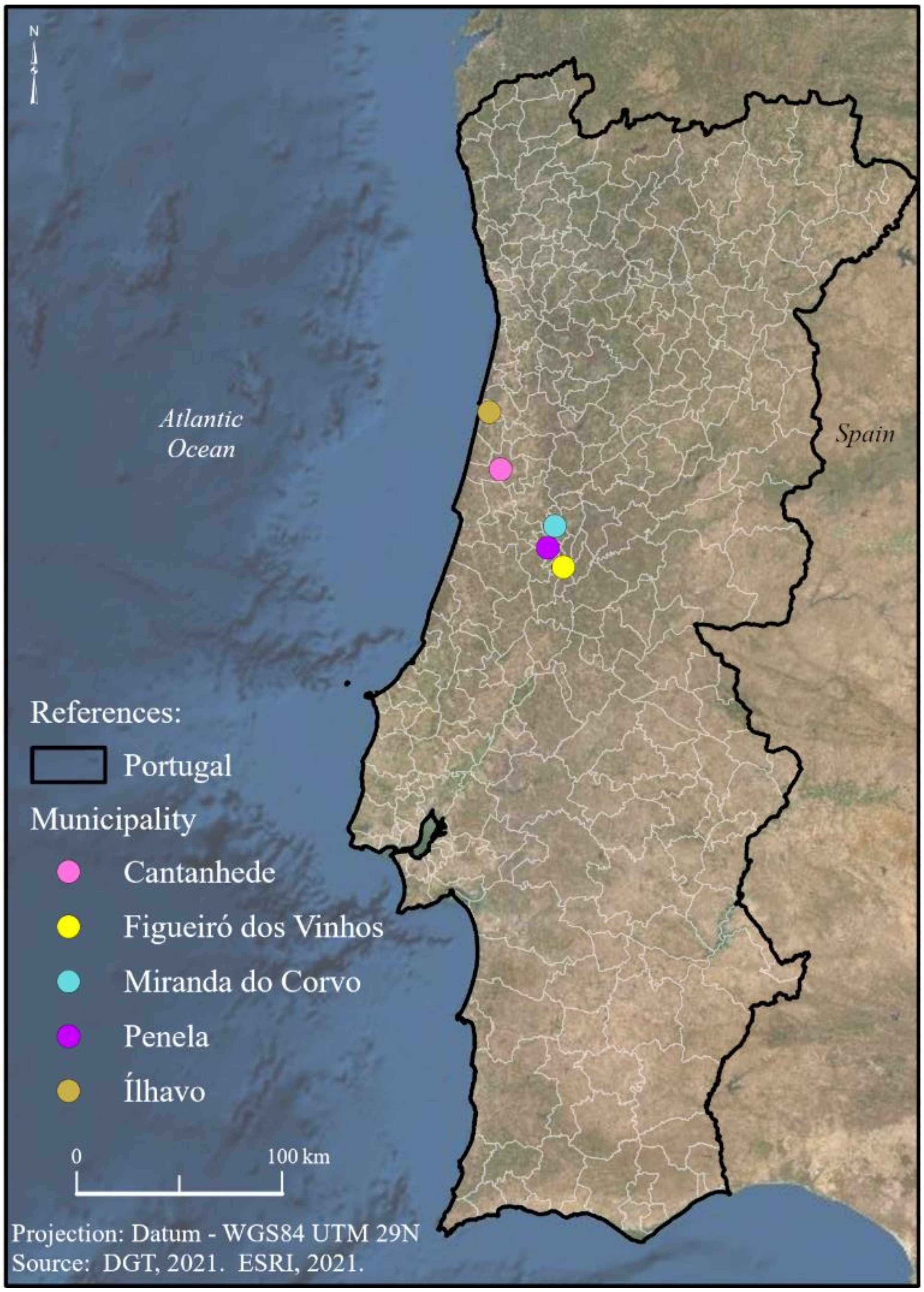
We selected five municipalities of Portugal (Figure 1) to test the predictive capacity of the model. Huang et al. [25] highlight the difficulty in validating maps using time series due to the lack of information available for past periods. Because of this same difficulty, the availability of a database capable of being used as validation, the choice of the test municipalities and the period of analysis were conditioned by the existence (or not) of those data.
The delimitation of the modelling area was made from a buffer of 100 m around the built areas, corresponding to the footage of the largest range of fuel management band established in the Decree-of-Law 124/2006. The total area with fuel analysed corresponds to 7311.88 hectares and the area without fuel corresponds to 9250.88 hectares, according to COSsim 2018.
2.5. Method
The method of analysis used to verify the vegetation changes around the built up areas is adapted from the model developed by Campagnolo et al. [30]. Initially proposed to verify burnt areas, the model searches for statistically significant differences between time series of satellite images, using a moving window. This semi-automatic model does not use training data, as the data from the neighbourhood of the study area are incorporated to avoid phenological variations of vegetation.
The analysis uses three values extracted from the time series. For each available image are checked: (i) the value of the NDVI in each pixel located within the study area; (ii) the mean value of the NDVI of the neighbouring pixels 500 m apart, located outside of the study area and in the same land cover; and (iii) the difference between these values.
The Welch t-test was applied for each of this information and each date of the time series. Welch t-test [38] is a variation of Student’s t-test and aims to find statistically significant differences between averages of two datasets of different sizes and variances. According to [39] the procedure of the t-test depends on the possibility that the variances of the samples can be considered equal. The hypothesis that allows considering equal variances is called homoscedasticity. The test is defined by
where x1 and x2 are the observed averages of the two samples, n1 and n2 are the sample size and Sp is the joint estimate of the standard deviation, which is calculated by
where S1 and S2 are the variances observed in samples 1 and 2. The degree of freedom associated with this statistic is n1 + n2 − 2.
If the variance of the samples is not considered equal the calculation of t is given by
In this case the degree of freedom is defined by the minimum value of (n1 − 1, n2 − 1).
Rogerson [39] points out that it is more appropriate to use the assumption of homoscedasticity, because when variances are not considered equal, it is more difficult to reject the null hypothesis.
Within this analysis, the null hypothesis (H0) assumes equality between the average of the two sets analysed—i.e., there are no differences between the means of the NDVI in the indicated period—thus showing that the area remained stable. The rejection of the null hypothesis suggests that there was some change, and this is identified by the p-value that is associated with the t value obtained for each analysed group. Since the p is less than or equal to a threshold, e.g., 0.05, the null hypothesis is rejected, and it is obtained that there was a statistically change in that period. The indication if there was a decrease in the NDVI is associated with the value of t when it presents values below zero.
The Welch t-test identifies significant differences between the mean value of two sets with different sizes and variances. These sets are defined by a time window applied before and after each date. The current date is included in the ‘before’ group. These groups have a minimum limit of 2 dates and a maximum of 8 dates and the moving time window is established in 60 days, to minimise problems in the months where there are few or no images with valid values, e.g., because of the presence of clouds.
The identification of a change occurs when the t-test points the significant difference for the value of ‘pixel (i)’ and the value of the ‘difference (iii)’ and not the ‘mean (ii)’ on the same date. Here, we only aim to identify changes that indicate the decrease of the NDVI value and this is associated with the negative values of t. Obeying these criteria, for each date of the analysed image a binary raster is generated where the pixels are classified with the value (1) where changes occur and value (0) in the unchanged areas
The resulting rasters are stacked to identify the changes between January and September 2020. To ensure that are sufficient images for the good functioning of the model at the beginning and end of the time series, we use images from the previous and subsequent months of the period analysed as a safety margin. The choice for this period is due to two main reasons. First, the data available for validation fits this period and, second, the deadlines for the management of the fuel bands set out in Decree-of-Law 124/2006.
To prevent a change from being recorded more than once, we identified the change only on the first date on which a significant difference occurs. To improve the predictive capacity of the model, two levels of significance were tested: p-value ≤ 0.05 and p-value ≤ 0.0005. The proposed model was developed in Python language, a free-access programming resource that allows great replicability.
The data available to validate the model was obtained within the National Republican Guard (Guarda Nacional Republicana—GNR) and consists of a database containing information on the monitoring of fuel management bands. This dataset is not available for the general public and therefore we just use the data made available by GNR. Nonetheless, fires occurrences in mainland Portugal are positively autocorrelated, showing higher prevalence in the north territory of the Tagus River [40]. Therefore, using the municipalities of Cantanhede, Figueiró dos Vinhos, Ílhavo, Miranda do Corvo, and Penela, as validation areas seems adequate.
To do the monitoring, GNR visits certain locations to verify whether there has been fuel management actions inside the fuel management bands. From this, the information indicating compliance or non-compliance with the law on management actions is stored. The surveys took place between February and August 2020 and has a total of 293 registries.
The validation consists in a 2 × 2 confusion matrix. To create it, GNR dataset were intersected with the COSsim 2018 and after that with the change raster generated by the model. This allows checking whether the point is in an area ‘with fuel’ or ‘without fuel’ and whether it has changed or not within the analysed period, according to the model generated. The established confusion matrix allows to access four values:
- True positive (TP), model records value (1), land cover is ‘fuel’ and the situation of the point indicates ‘compliance’.
- False positive (FP), model records value (1), land cover is ‘fuel’ and the situation at the point is different from ‘compliance’.
- True negative (TN), model records value (0), land cover is ‘fuel’ and the situation of the point is different from ‘compliance’.
- False negative (FN), model records value (0), land cover is ‘fuel’ and the situation of the point indicates ‘compliance’.
3. Results and Discussion
For the p-value limit of 0.05, the overall accuracy was 53.24% with a confidence interval of 1.97%. The accuracy was higher for the detection of no-changes events, 74.29%, with a confidence interval of 1.72% while in the detection of changes it was 33.99% with a confidence interval of 1.87%. The recall was higher in the detection of changes, 59.09%, with a confidence interval of 1.94%, for the not-changes was obtained 50.70% with a confidence interval of 1.97%. The F1-score showed better results for no-changes events, 60.29%, with a confidence interval of 1.93%, while for the events of changes it was 43.15% with a confidence interval of 1.95% (Table 2).
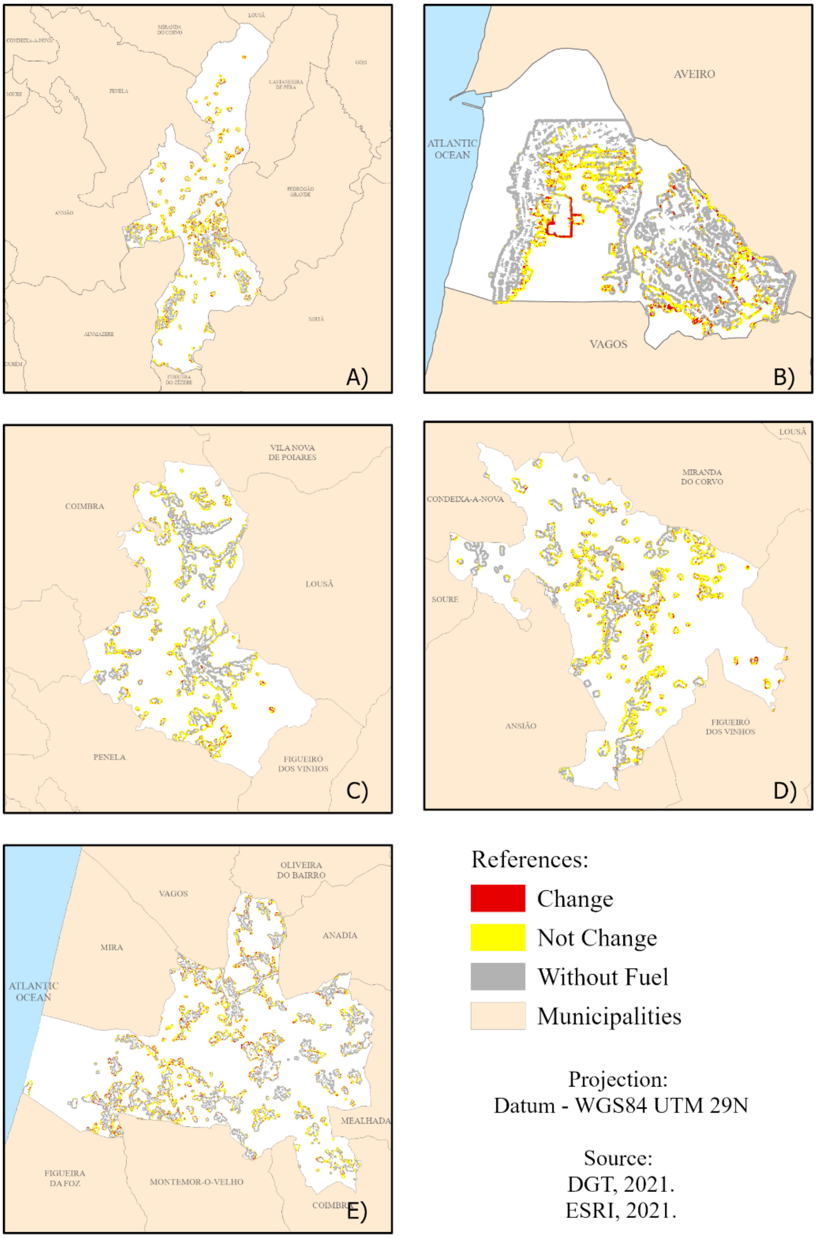
Figure 2 show the change maps with this p-value limit for all municipalities. The same maps can be found in large format in (Supplementary Materials Figures S1–S5).
For the model with the p-value limit of 0.0005, the overall accuracy was 64.85% with a confidence interval of 1.88%. The model showed a higher predictive capacity to detect no-changes in all verified metrics, as well as the associated confidence intervals were also lower. The accuracy obtained in the no-changes events was 71.43% with a confidence interval of 1.78% and for the events of changes, it was 36.36% with a confidence interval of 1.90%. The recall of 82.93% obtained for the detection of no-changes, the best value obtained by the model, presented a confidence interval of 1.48%, however, to detect changes the recall value obtained was the worst of the model, 22.73%, with a confidence interval of 1.65%. The F1-score was 76.75% in the no-changes events and 27.97% in the events of changes. The confidence intervals associated with these values were 1.66% and 1.77% respectively.
The rational of using two p-value limits to identify the changes was to improve the predictive capacity of the model and reduce false positive events. The results obtained by lowering the significance threshold from 0.05 to 0.0005 (Table 2 and Table 3) corroborated this hypothesis, showing an increase of approximately 11% in the overall accuracy of the model, from 53.24% to 64.85%. The results presented by [31] also recorded this same behaviour of increasing accuracy as the p-value threshold decreased.
The calculation of the confidence interval shows the variation rate that may exist within the results, i.e., their reliability. The model presented low confidence interval rates, indicating that the results obtained may vary little above or below from that obtained.
Figure 3 show the change maps with p-value limit 0.0005 for all municipalities. The same maps can be found in large format in (Supplementary Materials Figures S6–S10).
The 64.85% of the overall accuracy obtained by the developed model is low when compared to other models developed to detect changes in vegetation. Change detection algorithms such as LandTrendr [27] or VCT [25] showed higher overall accuracy. For LandTrendr the authors reported accuracy above 85%, while for VCT is stated an accuracy higher than 75%. The model developed by [26] registered a general accuracy higher than 90%, but because it is a model based on pre-established limits according to the spectral characteristics of the area analysed, this accuracy can change according to the study area. Concerning the models for detecting changes applied in Portugal, one can find the works of [42] to estimate the increase in vegetation biomass after fires in the north of the country, where the overall accuracy of 79.6% was recorded and of [31], in the search for vegetation cuts around the road network which yielded an accuracy of 79% for an annual temporal cut-off and 98% for a monthly temporal cut-off.
The relatively low values associated with precision, recall and F1-score metrics obtained in our model are associated with the small number of true positive events found. This is related to false positive and false negative events. There are some possible explanations of why we found these false events.
False positives are associated with: (i) when the cleansing of the vegetation was carried out after the field visit and audit carried out by the GNR. This can be attributed to the standards of items 5, 6, 12, and 13 of Article 15 of Decree-of-Law 124/2016, which say that in the case of fuel management is not done by 30 April the municipality council will be able to proceed itself with the management of fuel of the area; and (ii) the model may find statistically significant differences that are not related to the removal of vegetation per se. This can result from the natural reflectance of vegetation that is not constant and undergoes variations throughout the year. Spadoni [34] presented intra-annual variation of the NDVI in conifers, broad-leaved species and grassland in the north, centre and south of Italy, it is observed that the behaviour of the spectral signal was like that presented by [43] when analysing the annual variation of vegetation in the central part of mainland Portugal. Both studies, it is verified that there is a natural decay in the value of the NDVI in some types of vegetation in the period between January and September and this decay can be identified as alteration, despite the 60-day time window used to minimise these seasonal effects. Additionally, small signal noises or constant observations with the presence of clouds may interfere with the prediction of the model.
False negatives are associated with some characteristics of how fuel management should be carried out, as described in the Annex to Decree-of-Law 124/2016, which may not be captured by Sentinel-2. For instance, regarding isolated tree elements, which may be close to buildings, the spatial resolution of the data used limits the precise identification of the tree, making it difficult to identify this type of fuel management using Sentinel-2. Additionally, the removal of branches near the soil or cut the vegetation below the trees may not significantly interfere in the canopy of the vegetation fragment. This indicates that the variation of the NDVI may be small to be detected by the model.
Regarding the grassland stratum [28] shows that the decrease in the NDVI after cutting the high grass is in the order of 0.2, but it recovers 0.1 in the period between 8 and 10 days after the cut. Due to this rapid recovery of the NDVI value, grass-containing land cleaning events may go unnoticed because (a) no valid images are available, without cloud cover, on dates close to the vegetation removal events and (b) the NDVI variation in the period near the cut does not interfere significantly in the set analysed in the Welch t-test. These small changes, undetected by the satellite, are easier to identify on a field visit. Therefore, a GNR supervisor can identify fuel management ‘compliances’ that go unnoticed in the model.
Another factor that can interfere with the good functioning of the model is the temporality of the land cover map used. COSsim 2018 was prepared for the interval between September 2017 and October 2018. The proposed model used the available 2020 images, which indicates that some areas mapped in COSsim may already have changed. With this, we can be applying the model to an area that in the official mapping was considered fuel and today it is no longer. The opposite is also true.
Our results show that this model can be used to identify areas that need management, either by private individuals or by public entities, as well as to assist in the planning of supervision by the competent agencies. The elaborated model has the potential to be used on a national scale to verify changes in the fuel management bands.
4. Conclusions
The work carried out was satisfactory for the achievement of the desired objectives. Although the overall accuracy of the obtained model was 64.85%, relatively lower than that found in the literature consulted [25,27,31]. With the methodology used, it was possible to identify areas where interventions occurred in the fuel management bands. Above all, we obtained high predictive capacity to identify areas where there were no interference with vegetation, indicated by the precision of 71.43% and recall of 82.93%. This fact could be useful to find the areas where interventions must be done, optimizing the process in terms of cost and efficiency.
The NDVI obtained from Sentinel-2 Level-2A images proved to be effective in identifying changes in fuel management bands. We can list two other advantages when using Sentinel-2 images for this type of analysis: (i) the high availability of images due to temporal resolution and (ii) because they are made available free of charge.
This study concludes that the approach on this topic is far from being closed, but we believe that the model proposed here has the potential to improve the discussions on this topic. The knowledge applied in the development of the model proposed here can be used as a basis for new approaches and assists directly or indirectly in the search to map changes in vegetation.
For future approaches, we stress that new forms and sources of data for validation can be added, and the prospect of COSsim being produced annually can minimise the effects of the time gap. To solve the problem with clouds or no data in the images, could be incorporated images from other satellites, like: Sentinel-1 or Landsat, but in this case the spatial resolution problems is not solved. Another possibility is to use satellite images with higher spatial resolution than Sentinel-2, and/or to incorporate data from other technologies, such as unmanned aerial vehicles (UAV), radar or LiDAR data, to identify details that presently go unnoticed. However, using UAV or LiDar data is more expensive and the data collection time is longer.
Supplementary Materials
The following supporting information can be downloaded at: https://0-www-mdpi-com.brum.beds.ac.uk/article/10.3390/app12052294/s1. Figure S1: Changes detected in Cantanhede with p-value ≤ 005; Figure S2: Changes detected in Figueiro dos Vinhos with p-value ≤ 005; Figure S3: Changes detected in Ilhavo with p-value ≤ 005; Figure S4: Changes detected in Miranda do Corvo with p-value ≤ 005; Figure S5: Changes detected in Penela with p-value ≤ 005; Figure S6: Changes detected in Cantanhede with p-value ≤ 00005; Figure S7: Changes detected in Figueiro dos Vinhos with p-value ≤ 00005; Figure S8: Changes detected in Ilhavo with p-value ≤ 00005; Figure S9: Changes detected in Miranda do Corvo with p-value ≤ 00005 and Figure S10: Changes detected in Penela with p-value ≤ 00005.
Author Contributions
B.B.: conceptualisation, methodology, software, validation, formal analysis, research, curatorship of data, writing—preparation of the original sketch, writing—review and editing. H.C.: resources, visualisation, supervision, project administration, writing—review and editing. J.R.: conceptualisation, methodology, validation, writing—review and editing, supervision. M.C.: conceptualisation, methodology, resources, visualisation, supervision, project administration, financing acquisition. All authors have read and agreed to the published version of the manuscript.
Funding
This research was funded by Portuguese Foundation for Science and Technology, I.P. (FCT), under the framework of the Project “FORESTER—Data fusion of sensor networks and fire spread modelling for decision support in forest fire suppression” [name of funder] grant number PCIF/SSI/0102/2017. The APC was funded by the Research Unit UIDB/00295/2020 and UIDP/00295/2020.
Institutional Review Board Statement
Not applicable.
Informed Consent Statement
Not applicable.
Acknowledgments
We acknowledge the GEOMODLAB—Laboratory for Remote Sensing, Geographical Analysis and Modeling—of the Center of Geographical Studies/IGOT. We would also like to thank to the editor and the anonymous reviewers that contributed to the improvement of this paper. The authors thank to the Portuguese Guarda Nacional Republicana (GNR) for providing the validation data. Value-added data processed by CNES for the Theia data centre www.theia-land.fr using Copernicus products. The satellite image pre-processing uses algorithms developed by Theia’s Scientific Expertise Centers.
Conflicts of Interest
The authors declare that they have no known competing financial interests or personal relationships that could have appeared to influence the work reported in this paper.
References
- de Castro, A.L.C.; Calheiros, L.B.; Cunha, M.I.R.; Bringel, M.L.N.C. Manual de Desastres Naturais. Brasilia: Ministério da Integração Nacional. 2003. Available online: https://www.campinas.sp.gov.br/governo/secretaria-de-governo/defesa-civil/desastres_naturais_vol1.pdf (accessed on 20 October 2021).
- Bergonse, R.; Oliveira, S.; Gonçalves, A.; Nunes, S.; da Câmara, C.; Zêzere, J.L. A combined structural and seasonal approach to assess wildfire susceptibility and hazard in summertime. Nat. Hazards 2021, 106, 2545–2573. [Google Scholar] [CrossRef]
- ProCiv. Autoridade Nacional de Emergência e Proteção Civil. 2022. Available online: http://www.prociv.pt/pt-pt/RISCOSPREV/RISCOSNAT/INCENDIOSRURAIS/Paginas/default.aspx (accessed on 11 January 2022).
- Gómez-González, S.; Ojeda, F.; Fernandes, P.M. Portugal and Chile: Longing for sustainable forestry while rising from the ashes. Environ. Sci. Policy 2018, 81, 104–107. Available online: https://0-www-sciencedirect-com.brum.beds.ac.uk/science/article/pii/S1462901117307694 (accessed on 10 February 2022). [CrossRef]
- Sánchez-Benítez, A.; García-Herrera, R.; Barriopedro, D.; Sousa, P.M.; Trigo, R.M. June 2017: The Earliest European Summer Mega-Heatwave of Reanalysis Period. Geophys. Res. Lett. 2018, 45, 1955–1962. [Google Scholar] [CrossRef]
- Turco, M.; Jerez, S.; Augusto, S.; Tarín-Carrasco, P.; Ratola, N.; Jiménez-Guerrero, P.; Trigo, R.M. Climate drivers of the 2017 devastating fires in Portugal. Sci. Rep. 2019, 9, 13886. [Google Scholar] [CrossRef] [PubMed]
- Oliveira, S.; Gonçalves, A.; Zêzere, J.L. Reassessing wildfire susceptibility and hazard for mainland Portugal. Sci. Total Environ. 2021, 762, 143121. Available online: https://0-www-sciencedirect-com.brum.beds.ac.uk/science/article/pii/S0048969720366511 (accessed on 10 February 2022). [CrossRef] [PubMed]
- Tonini, M.; D’Andrea, M.; Biondi, G.; Degli Esposti, S.; Trucchia, A.; Fiorucci, P. A Machine Learning-Based Approach for Wildfire Susceptibility Mapping. The Case Study of the Liguria Region in Italy. Geosciences 2020, 10, 105. [Google Scholar] [CrossRef] [Green Version]
- Commission, E.; Centre, J.R.; Gazzard, R.; Müller, M.; Sciunnach, R.; Pecl, J.; Konstantinov, V.; Sbirnea, R.; Cruz, M.; Chassagne, F.; et al. Forest Fires in Europe, Middle East and North Africa 2018; Publications Office of the European Union: Luxembourg, 2019. [Google Scholar]
- Meira Castro, A.C.; Nunes, A.; Sousa, A.; Lourenço, L. Mapping the Causes of Forest Fires in Portugal by Clustering Analysis. Geosciences 2020, 10, 53. [Google Scholar] [CrossRef] [Green Version]
- Moreira, F.; Viedma, O.; Arianoutsou, M.; Curt, T.; Koutsias, N.; Rigolot, E.; Barbati, A.; Corona, P.; Vaz, P.; Xanthopoulos, G.; et al. Landscape—Wildfire interactions in southern Europe: Implications for landscape management. J. Environ. Manag. 2011, 92, 2389–2402. Available online: https://0-www-sciencedirect-com.brum.beds.ac.uk/science/article/pii/S0301479711002258 (accessed on 10 February 2022). [CrossRef] [PubMed] [Green Version]
- Nunes, A.N.; Lourenço, L.; Meira, A.C.C. Exploring spatial patterns and drivers of forest fires in Portugal (1980–2014). Sci. Total Environ. 2016, 573, 1190–1202. Available online: https://0-www-sciencedirect-com.brum.beds.ac.uk/science/article/pii/S0048969716305460 (accessed on 10 February 2022). [CrossRef]
- Tedim, F.; Remelgado, R.; Borges, C.; Carvalho, S.; Martins, J. Exploring the occurrence of mega-fires in Portugal. For. Ecol. Manag. 2013, 294, 86–96. Available online: https://0-www-sciencedirect-com.brum.beds.ac.uk/science/article/pii/S0378112712004379 (accessed on 10 February 2022). [CrossRef]
- Hirschmugl, M.; Gallaun, H.; Dees, M.; Datta, P.; Deutscher, J.; Koutsias, N.; Schardt, M. Methods for Mapping Forest Disturbance and Degradation from Optical Earth Observation Data: A Review. Curr. For. Rep. 2017, 3, 32–45. [Google Scholar] [CrossRef] [Green Version]
- Zhu, Z. Change detection using landsat time series: A review of frequencies, preprocessing, algorithms, and applications. ISPRS J. Photogramm. Remote Sens. 2017, 130, 370–384. [Google Scholar] [CrossRef]
- Liu, D.; Cai, S. A Spatial-Temporal Modeling Approach to Reconstructing Land-Cover Change Trajectories from Multi-Temporal Satellite Imagery. Ann. Assoc. Am. Geogr. 2012, 102, 1329–1347. [Google Scholar] [CrossRef]
- Cunningham, S.; Rogan, J.; Martin, D.; DeLauer, V.; McCauley, S.; Shatz, A. Mapping land development through periods of economic bubble and bust in Massachusetts using Landsat time series data. GISci. Remote Sens. 2015, 52, 397–415. [Google Scholar] [CrossRef]
- Powell, S.L.; Cohen, W.B.; Yang, Z.; Pierce, J.D.; Alberti, M. Quantification of impervious surface in the Snohomish Water Resources Inventory Area of Western Washington from 1972–2006. Remote Sens. Environ. 2008, 112, 1895–1908. [Google Scholar] [CrossRef] [Green Version]
- Hayes, D.J.; Sader, S.A. Comparison of change-detection techniques for monitoring tropical forest clearing and vegetation regrowth in a time series. Photogramm. Eng. Remote Sens. 2001, 67, 1067–1075. [Google Scholar]
- Bolton, D.K.; Coops, N.C.; Wulder, M.A. Characterizing residual structure and forest recovery following high-severity fire in the western boreal of Canada using Landsat time-series and airborne lidar data. Remote Sens. Environ. 2015, 163, 48–60. [Google Scholar] [CrossRef]
- Coppin, P.; Jonckheere, I.; Nackaerts, K.; Muys, B.; Lambin, E. Digital change detection methods in ecosystem monitoring: A review. Int. J. Remote Sens. 2004, 25, 1565–1596. [Google Scholar] [CrossRef]
- Viana, C.M.; Girão, I.; Rocha, J. Long-term satellite image time-series for land use/land cover change detection using refined open source data in a rural region. Remote Sens. 2019, 11, 1104. [Google Scholar] [CrossRef] [Green Version]
- Banskota, A.; Kayastha, N.; Falkowski, M.J.; Wulder, M.A.; Froese, R.E.; White, J.C. Forest Monitoring Using Landsat Time Series Data: A Review. Can. J. Remote Sens. 2014, 40, 362–384. [Google Scholar] [CrossRef]
- Kuenzer, C.; Dech, S.; Wagner, W. Remote Sensing Time Series Revealing Land Surface Dynamics: Status Quo and the Pathway Ahead. In Remote Sensing Time Series Revealing Land Surface Dynamics; Springer International Publisher: Berlin, Germany, 2015; pp. 1–24. [Google Scholar]
- Huang, C.; Goward, S.N.; Masek, J.G.; Thomas, N.; Zhu, Z.; Vogelmann, J.E. An automated approach for reconstructing recent forest disturbance history using dense Landsat time series stacks. Remote Sens. Environ. 2010, 114, 183–198. [Google Scholar] [CrossRef]
- Koutsias, N.; Pleniou, M.; Mallinis, G.; Nioti, F.; Sifakis, N.I. A rule-based semi-automatic method to map burned areas: Exploring the USGS historical Landsat archives to reconstruct recent fire history. Int. J. Remote Sens. 2013, 34, 7049–7068. [Google Scholar] [CrossRef]
- Kennedy, R.E.; Yang, Z.; Cohen, W.B. Detecting trends in forest disturbance and recovery using yearly Landsat time series: 1. LandTrendr—Temporal segmentation algorithms. Remote Sens. Environ. 2010, 114, 2897–2910. [Google Scholar] [CrossRef]
- Kolecka, N.; Ginzler, C.; Pazur, R.; Price, B.; Verburg, P.H. Regional Scale Mapping of Grassland Mowing Frequency with Sentinel-2 Time Series. Remote Sens. 2018, 10, 1221. [Google Scholar] [CrossRef] [Green Version]
- Hamunyela, E.; Verbesselt, J.; Herold, M. Using spatial context to improve early detection of deforestation from Landsat time series. Remote Sens. Environ. 2016, 172, 126–138. [Google Scholar] [CrossRef]
- Campagnolo, M.L.; Oom, D.; Padilla, M.; Pereira, J.M.C. A patch-based algorithm for global and daily burned area mapping. Remote Sens. Environ. 2019, 232, 111288. [Google Scholar] [CrossRef]
- Aubard, V.; Pereira-Pires, J.E.; Campagnolo, M.L.; Pereira, J.M.C.; Mora, A.; Silva, J.M.N. Fully Automated Countrywide Monitoring of Fuel Break Maintenance Operations. Remote Sens. 2020, 12, 2879. [Google Scholar] [CrossRef]
- Baetens, L.; Desjardins, C.; Hagolle, O. Validation of copernicus Sentinel-2 cloud masks obtained from MAJA, Sen2Cor, and FMask processors using reference cloud masks generated with a supervised active learning procedure. Remote Sens. 2019, 11, 433. [Google Scholar] [CrossRef] [Green Version]
- Theia—Land Data Center. 2022. Available online: https://theia.cnes.fr/atdistrib/rocket/#/home (accessed on 11 January 2022).
- Spadoni, G.L.; Cavalli, A.; Congedo, L.; Munafo, M. Analysis of Normalized Difference Vegetation Index (NDVI) multi-temporal series for the production of forest cartography. Remote Sens. Appl. Soc. Environ. 2020, 20, 100419. [Google Scholar] [CrossRef]
- Hislop, S.; Jones, S.; Soto-Berelov, M.; Skidmore, A.; Haywood, A.; Nguyen, T.H. Using landsat spectral indices in time-series to assess wildfire disturbance and recovery. Remote Sens. 2018, 10, 460. [Google Scholar] [CrossRef] [Green Version]
- Cartografia das Áreas Edificadas e da Interface Urbano-Rural Para Portugal Continental. 2018. Available online: http://mapas.dgterritorio.pt/viewer/areasedificadas/Info/AreasEdificadasREADME_1Junho2020.pdf (accessed on 11 January 2022).
- ICNF. Áreas Ardidas Por Tipo de Ocupação do solo (1996–2014). 2015. Available online: http://www2.icnf.pt/portal/florestas/dfci/Resource/doc/estat/area-ardida-1996-a-2014 (accessed on 17 August 2021).
- Welch, B.L. The generalization of ‘student’s’ problem when several different population variances are involved. Biometrika 1947, 34, 28–35. [Google Scholar] [CrossRef]
- Rogerson, P.A. Métodos Estatísticos Para Geografia: Um Guia Para o Estudante, 3rd ed.; Carvalho, P.B., Rigotti, J.R., Eds.; Bookman: Porto Alegre, Brazil, 2012. [Google Scholar]
- Bergonse, R.; Oliveira, S.; Zêzere, J.L.; Moreira, F.; Ribeiro, P.F.; Leal, M.; e Santos, J.M.L. Biophysical controls over fire regime properties in Central Portugal. Sci Total Environ. 2022, 810, 152314. Available online: https://0-www-sciencedirect-com.brum.beds.ac.uk/science/article/pii/S0048969721073903 (accessed on 10 February 2022). [CrossRef]
- Baraldi, A.; Puzzolo, V.; Blonda, P.; Bruzzone, L.; Tarantino, C. Automatic spectral rule-based preliminary mapping of calibrated landsat TM and ETM+ images. IEEE Trans. Geosci. Remote Sens. 2006, 44, 2563–2585. [Google Scholar] [CrossRef] [Green Version]
- Aranha, J.; Enes, T.; Calvão, A.; Viana, H. Shrub biomass estimates in former burnt areas using sentinel 2 images processing and classification. Forests 2020, 11, 555. [Google Scholar] [CrossRef]
- Pereira-Pires, J.E.; Aubard, V.; Ribeiro, R.A.; Fonseca, J.M.; Silva, M.N.; Mora, A. Semi-Automatic Methodology for Fire Break Maintenance Operations Detection with Sentinel-2 Imagery and Artificial Neural Network. Remote Sens. 2020, 12, 909. [Google Scholar] [CrossRef] [Green Version]
Figure 1.
Localization of the selected five municipalities.

Figure 2.
Changes detected in: (A) Figueiró dos Vinhos, (B) Ílhavo, (C) Miranda do Corvo, (D) Penela, (E) Cantanhede, with p-value ≤ 0.05.
Figure 2.
Changes detected in: (A) Figueiró dos Vinhos, (B) Ílhavo, (C) Miranda do Corvo, (D) Penela, (E) Cantanhede, with p-value ≤ 0.05.

Figure 3.
Changes detected in: (A) Figueiró dos Vinhos, (B) Ílhavo, (C) Miranda do Corvo, (D) Penela, (E) Cantanhede, with p-value ≤ 0.0005.
Figure 3.
Changes detected in: (A) Figueiró dos Vinhos, (B) Ílhavo, (C) Miranda do Corvo, (D) Penela, (E) Cantanhede, with p-value ≤ 0.0005.


Table 1.
COSsim 2018 land cover classes.
| Code | Class Name | Study Area Municipalities (%) | Study Area 100 m Buffer (%) | Mainland Portugal (%) | Fuel |
|---|---|---|---|---|---|
| 100 | Artificial land | 5.24 | 2.32 | 3.10 | No |
| 200 | Agriculture | 19.64 | 26.90 | 35.19 | No |
| 420 | Spontaneous grassland | 3.78 | 3.63 | 8.28 | No |
| 311 | Cork oak and holm oak | - | - | 9.42 | No |
| 312 | Eucalyptus | 29.02 | 33.92 | 8.57 | Yes |
| 313 | Other broadleaved forests | 8.66 | 7.81 | 4.07 | Yes |
| 321 | Maritime pine | 8.27 | 4.32 | 4.74 | Yes |
| 322 | Stone pine | 0.05 | 0.02 | 1.59 | Yes |
| 323 | Other conifers | 0.11 | 0.11 | 0.22 | Yes |
| 410 | Bush | 16.91 | 16.99 | 17.60 | Yes |
| 500 | Bare soil | 6.80 | 3.49 | 3.52 | No |
| 610 | Wetlands | 0.49 | 0.13 | 0.25 | No |
| 620 | Water | 1.04 | 0.37 | 3.45 | No |
Table 2.
Validation with p-value ≤ 0.05.
| Statistical Metrics | Matrix | ||||
|---|---|---|---|---|---|
| (C) | (NC) | (C) | (NC) | ||
| Precision | 33.99% ± 1.87% * | 74.29% ± 1.72% * | (C) | 52 | 101 |
| Recall | 59.09% ± 1.94% * | 50.73% ± 1.97% * | |||
| F1-Score | 43.15% ± 1.95% * | 60.29% ± 1.93% * | (NC) | 36 | 104 |
| Overall Accuracy | 53.24% ± 1.97% * | ||||
* Confidence Interval; C—Change; NC—Not Change.
Table 3.
Validation with p-value ≤ 0.0005.
| Statistical Metrics | Matrix | ||||
|---|---|---|---|---|---|
| (C) | (NC) | (C) | (NC) | ||
| Precision | 36.36% ± 1,90% * | 71.43% ± 1.78% * | (C) | 20 | 35 |
| Recall | 22.73% ± 1,65% * | 82.93% ± 1.48% * | |||
| F1-score | 27.97% ± 1,77% * | 76.75% ± 1.66% * | (NC) | 68 | 170 |
| Overall accuracy | 64.85% ± 1.88% * | ||||
* Confidence Interval; C—Change; NC—Not Change.
Publisher’s Note: MDPI stays neutral with regard to jurisdictional claims in published maps and institutional affiliations. |
© 2022 by the authors. Licensee MDPI, Basel, Switzerland. This article is an open access article distributed under the terms and conditions of the Creative Commons Attribution (CC BY) license (https://creativecommons.org/licenses/by/4.0/).
Share and Cite
MDPI and ACS Style
Barbosa, B.; Rocha, J.; Costa, H.; Caetano, M. Uncovering Vegetation Changes in the Urban–Rural Interface through Semi-Automatic Methods. Appl. Sci. 2022, 12, 2294. https://0-doi-org.brum.beds.ac.uk/10.3390/app12052294
AMA Style
Barbosa B, Rocha J, Costa H, Caetano M. Uncovering Vegetation Changes in the Urban–Rural Interface through Semi-Automatic Methods. Applied Sciences. 2022; 12(5):2294. https://0-doi-org.brum.beds.ac.uk/10.3390/app12052294
Chicago/Turabian StyleBarbosa, Bruno, Jorge Rocha, Hugo Costa, and Mário Caetano. 2022. "Uncovering Vegetation Changes in the Urban–Rural Interface through Semi-Automatic Methods" Applied Sciences 12, no. 5: 2294. https://0-doi-org.brum.beds.ac.uk/10.3390/app12052294
Note that from the first issue of 2016, this journal uses article numbers instead of page numbers. See further details here.