Reconfigurable Fault-Tolerant Control for Spacecraft Formation Flying Based on Iterative Learning Algorithms

Abstract

This paper investigates the issues of iterative learning algorithm-based robust thruster fault reconstruction and reconfigurable fault-tolerant control for spacecraft formation flying systems subject to space perturbations. Motivated by sliding mode methodology, a novel iterative learning observer (ILO) was developed to robustly reconstruct the thruster faults. Based on the fault signals obtained from the ILO, a learning output–feedback fault-tolerant control (LOF²TC) approach was explored such that the closed-loop spacecraft formation configuration was accurately maintained in the presence of space perturbations and thruster faults. Numerical simulations were employed to demonstrate the effectiveness and superiority of the proposed ILO-based fault-reconstructing approach and LOF²TC-based configuration maintenance approach for spacecraft formation flying systems.

1. Introduction

As the research hotspot in the field of spaceflight technology, which has been intensively studied in the past decade, spacecraft formation flying has been a key technology for lots of space missions, such as distributed aperture radar, earth monitoring, and deep space observation [1,2]. Compared with a large and complex spacecraft, a spacecraft formation flying system provides a multitude of benefits in space missions, including higher reconfiguration performance, higher reliability and redundancy, and low dependence on ground stations. Spacecraft formation control is regarded as the core technology for spacecraft formation flying with the diversification of space missions [3]. Therefore, spacecraft formation control techniques have been increasingly attracting the attention of scholars during the past two decades; many research results have been developed in the literature [4,5].

In on-orbit spacecraft formation flying systems, various perturbations, including solar radiation pressure, atmospheric drag, and the earth’s oblateness from the space environment, will result in drifts in both the formation configuration and the formation center. On the other hand, a spacecraft formation control system unavoidably manifests various types of unexpected anomalies and faults during on-orbit mission operations [6,7]. Faults may dramatically degrade the control performance properties to the point that formation configurations may be unsatisfactory for space missions, and could even result in the loss of control of an entire spacecraft formation control system. To guarantee the high control performance, reliability, and safety of spacecraft formation flying systems, fault diagnosis and fault-tolerant control (FTC) are challenging problems that need to be handled urgently for spacecraft formation flying systems in practice. In view of these, fault diagnosis and FTC for spacecraft formation control systems have attracted considerable attention in both research and practical applications during the past decade, and great progress has been achieved in recently published work in the literature [8,9,10,11,12,13,14,15,16].

In [8], fuzzy rule-based fault diagnosis approaches were proposed for the leader–follower spacecraft formation architecture. In [9], a fault detection and diagnosis approach, based on the Lur’e differential inclusion theory and fuzzy wavelet neural network, was proposed for the propulsion subsystem of spacecraft formation. In [10], based on the linear parameter varying technique, nonlinear observers were respectively explored to detect, isolate, and estimate actuator faults in a multi-satellite formation system, and less conservative linear matrix inequality (LMI) conditions were provided for observer design. In [11], a new sub-observers-based distributed cooperative state and fault estimation framework was proposed for a formation flight of satellites with unreliable relative state determination information resulting from external disturbances and actuator faults. In this framework, a series of sub-observers were selected and configured by a decision-making supervisor that cooperatively estimated the relative states and actuator faults. In [12], considering model uncertainties, time-varying disturbances and faults in spacecraft sensors and thrusters, a traditional sliding mode control algorithm, and a non-singular terminal sliding mode control algorithm were proposed for accurate formation configuration maintenance based on variable-structure control theory. To solve the fault-tolerant precise control problem of a satellite formation flying system with various uncertainties and external disturbances, the minimum sliding mode error feedback control approach was proposed based on the concept of equivalent control error to offset the J2 perturbation and smooth out the effect of the nonlinear switching control in [13]. In [14], a reconfigurable spacecraft formation FTC approach was designed based on a super-twisting sliding mode observer, which had strong robustness to measurement noise and J2 orbital perturbation. The reconfigurable FTC approach in different failure modes could effectively maintain the spacecraft formation configuration. In [15], a decentralized FTC algorithm was proposed for the three-inline array tethered spacecraft formation system. In [16], two new adaptive FTC algorithms were developed to estimate the effectiveness of the actuator, spacecraft masses, and the upper bound of external disturbances for spacecraft formation control systems that are subject to time-varying communication delays. It is noteworthy that robust fault reconstruction observer-based reconfigurable spacecraft formation FTC has not been considered in the existing literature, although fault reconstruction and spacecraft formation FTC have been separately addressed.

During the past decade, fault diagnosis and FTC based on iterative learning algorithms have been widely studied in time-delay systems, Takagi–Sugeno fuzzy systems, etc., [17,18,19], and applied in robotics and spacecraft systems [6,7]. Recently, iterative learning algorithms have been attracting much attention from aerospace scholars mainly because they can be applied to robust fault reconstruction and reconfigurable FTC for spacecraft systems. In [20], an ILO was designed to estimate the torque deviation for rigid spacecraft attitude stabilization in the presence of external disturbances and actuator faults. In [21], a novel ILO that could simultaneously reconstruct actuator faults and disturbances was developed for the attitude control of spacecrafts against actuator faults. In [22], two new non-linear ILO were suggested in order to robustly reconstruct effectiveness factors and bias faults of reaction wheels for spacecraft attitude control systems (ACSs) subject to space disturbance torques. In [23], a new fault diagnosis observer was proposed based on the iterative learning methodology to reconstruct actuator failures in real time for spacecraft ACSs in the presence of actuator failures, external disturbances, and actuator saturation. In [24], a novel Barrier Function-based ILO was designed to reconstruct the lumped disturbance, including multiple disturbances and failure torque, for spacecraft attitude stabilization. However, so far few research results on iterative learning algorithms have been focused on spacecraft formation flying systems. In addition, in comparison with the existing integrator-based adaptive algorithm, the algebraic iterative learning algorithm required less computation and no existence of derivatives at some time instants [21,22,25]. Therefore, the iterative learning algorithm was easier to implement in practice, especially when considering the limited storage and computing power for on-board computers in the spacecraft formation flying system. In light of these, there was a strong incentive for us to investigate iterative learning algorithm-based fault reconstruction and reconfigurable FTC for spacecraft formation flying systems.

Based on the above discussions, this paper investigates the issues of robust thruster fault reconstruction and reconfigurable fault tolerant control for a spacecraft formation flying system based on the iterative learning algorithms. Considering space perturbations and thruster faults, the relative orbital dynamics of spacecraft formation control systems are established. Considering the drawback in robustness of the existing ILOs [21,22,25] and the robustness of fault reconstruction against space perturbations in spacecraft formation flying systems, a novel ILO was proposed to robustly reconstruct thruster bias faults based on sliding mode methodology, and partial ILO-gain matrices could be conveniently solved by using LMI optimization techniques. Based on two iterative learning algorithms, a learning output–feedback fault-tolerant control (LOF²TC) scheme was explored so that accurate formation configuration maintenance could be fulfilled for spacecraft formation flying systems. Finally, simulation studies were provided to illustrate the effectiveness and superiority of the proposed robust fault reconstruction and reconfigurable fault tolerant control for spacecraft formation flying systems. In this paper, the main contributions that are worth emphasizing are summarized in the following three points.

(1)

Motivated by sliding mode methodology, a new ILO was designed for robust thruster bias fault reconstruction for spacecraft formation flying systems, subject to space perturbations. In addition, compared with the existing ILOs, a new ILO stability analysis methodology was provided in detail.

(2)

Based on two iterative learning algorithms, a new LOF²TC approach was explored for accurate spacecraft formation configuration maintenance in presence of space perturbations and possible uncertainties.

(3)

It is worth noting that iterative learning algorithms were not developed for spacecraft formation control systems. Therefore, the proposed ILO-based robust thruster fault reconstruction and LOF²TC approach provide an extension for spacecraft application.

The rest of this paper is organized as follows. In Section 2, the considered spacecraft formation control system model is established and the main problems are formulated. In Section 3, a new ILO is constructed to reconstruct actuator faults and estimate system states simultaneously, and the stability analysis for the proposed ILO is also derived in detail. In Section 4, the LOF²TC approach is presented for configuration maintenance under thruster faults, space perturbations, and possible uncertainties, and, then, its stability analysis is provided. In Section 5, simulation studies are presented, and Section 6 concludes this paper.

2. Problem Formulation

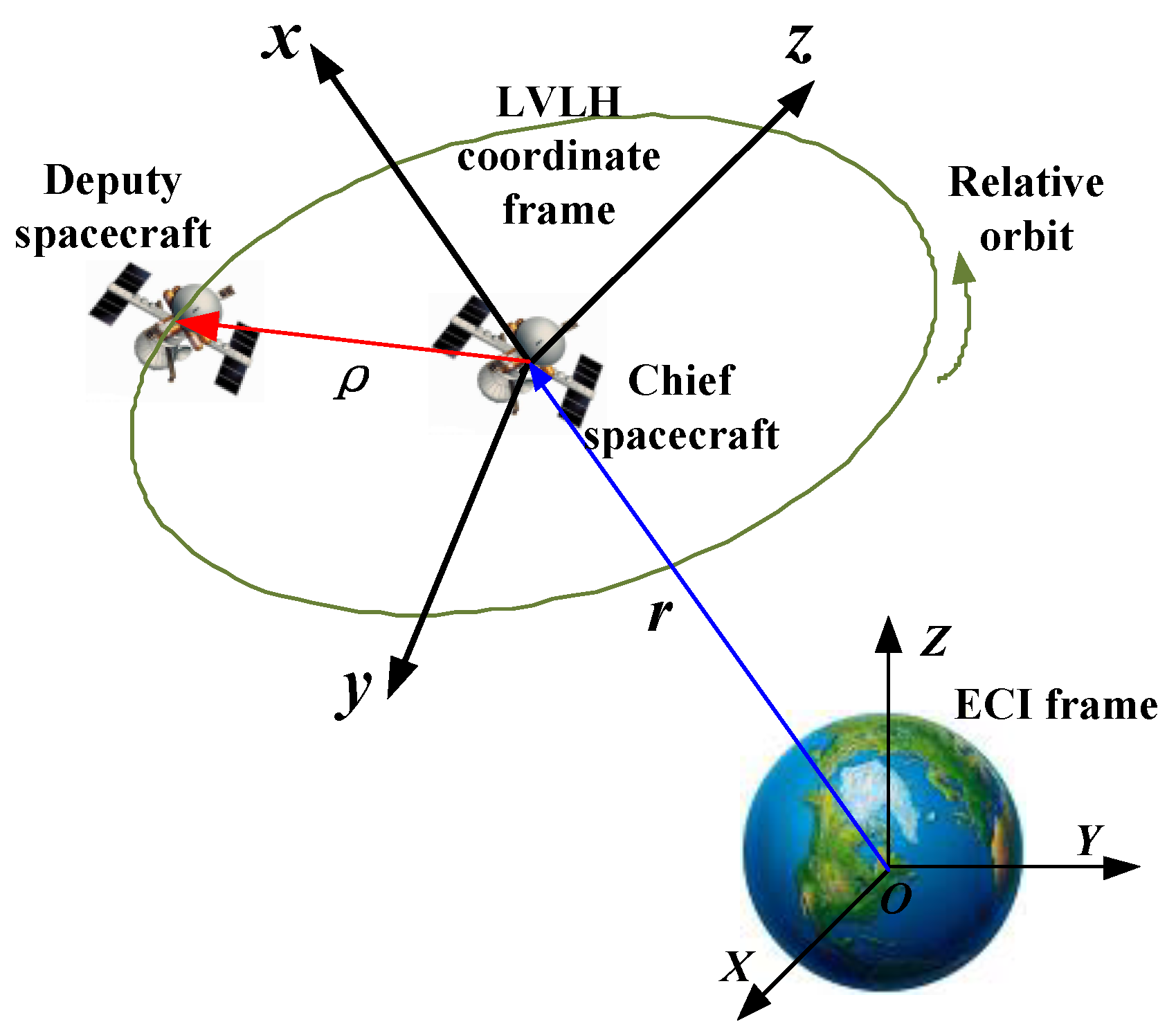
In this paper, it is assumed that the chief spacecraft runs in a circular orbit and formation configuration is short distance. As shown in Figure 1, the considered spacecraft formation flying system comprised a chief spacecraft and a deputy spacecraft. $r$ refers to the position vector of the chief spacecraft with respect to the earth-centered inertial (ECI) frame O-XYZ, which is attached to the center of the earth. The relative motion model for spacecraft formation flying was formulated in the local vertical and local horizontal (LVLH) coordinate frame that was fixed at the center of the chief spacecraft. In this frame, the x, y, and z components are referred to as radial direction, tangential direction, and normal direction, respectively.

Considering space perturbation, the linear C–W equation [9,26] describes the relative dynamic motion between the deputy spacecraft and the chief spacecraft and is as follows:

$$\{\begin{array}{l}\ddot{x}=2n\dot{y}+3n^{2}x+u_x+d_x\\ \ddot{y}=-2n\dot{x}+u_y+d_y\\ \ddot{z}=-n^{2}z+u_z+d_z\end{array}$$

(1)

where x, y, z are the components of relative position in each axis, n is the constant angular velocity of the chief spacecraft around the earth, and $u_i,i=x,y,z$ are the components of orbit control force provided by thrusters along each axis of the deputy spacecraft. $d_i,i=x,y,z$ are the components of space perturbation along each axis.

We define system state as $\dot{\mathit{q}}(t)={[x,\hspace{0.17em}y,\hspace{0.17em}z,\hspace{0.17em}\dot{x},\hspace{0.17em}\dot{y},\hspace{0.17em}\dot{z}]}^T$, and the relative motion equation in (1) can be written into the following state–space model.

$$\{\begin{array}{l}\dot{\mathit{q}}=\mathit{A}\mathit{q}+\mathit{B}\mathit{u}+\mathit{E}\mathit{d}\\ \mathit{y}=\mathit{C}\mathit{q}\end{array}$$

(2)

where the control input vector $\mathit{u}(t)={[u_x,\hspace{0.17em}{u}_y,\hspace{0.17em}{u}_z]}^T$, space perturbation $\mathit{d}(t)={[d_x,\hspace{0.17em}{d}_y,\hspace{0.17em}{d}_z]}^T$, and coefficient matrices are denoted by the following.

$$\mathit{A}=\left[\begin{array}{cc}{\mathit{0}}_3& {\mathit{I}}_3\\ {\mathit{A}}_1& {\mathit{A}}_2\end{array}\right], B=E=\left[\begin{array}{c}{\mathit{0}}_3\\ {\mathit{I}}_3\end{array}\right], \mathit{C}={\mathit{I}}_6, \mathrm{and} {\mathit{A}}_1=\left[\begin{array}{ccc}3n^2& 0& 0\\ 0& 0& 0\\ 0& 0& -n^2\end{array}\right], {\mathit{A}}_2=\left[\begin{array}{ccc}0& 2n& 0\\ -2n& 0& 0\\ 0& 0& 0\end{array}\right].$$

Considering the thruster bias fault, a fault-free spacecraft formation system (2) can be rewritten into the following form.

$$\{\begin{array}{l}\dot{\mathit{q}}=\mathit{A}\mathit{q}+\mathit{B}\mathit{u}+\mathit{E}\mathit{d}(t)+\mathit{H}\mathit{F}(t)\\ \mathit{y}=\mathit{C}\mathit{q}\end{array}$$

(3)

where $\mathit{F}(t)$ represents control force results from thruster faults and the fault distribution matrix $\mathit{H}=\mathit{B}$.

Assumption 1.

In this study, the space perturbation$\mathit{d}(t)$is assumed to be bounded, and it satisfies the following:

$$\Vert \mathit{d}(t)\Vert \le d_{\max }$$

(4)

where$d_{\max }$is a positive constant.

The main objective of this work was to develop robust thruster bias fault reconstruction and a learning output–feedback fault-tolerant tracking control approach for spacecraft formation flying systems based on iterative learning algorithms. For reconstructing thruster bias fault robustly, a novel ILO was explored for the spacecraft formation dynamics (3). Based on the faults reconstructed using the designed ILO, an LOF²TC approach was developed for the purpose of accurate spacecraft formation configuration maintenance.

3. Iterative Learning Observer-Based Thruster Fault Reconstruction Approach

3.1. Design of the Iterative Learning Observer

For reconstructing the thruster bias faults, the new continuous-time ILO was constructed for (3) in the following form,

$$\{\begin{array}{l}\dot{\widehat{\mathit{q}}}(t)=\mathit{A}\widehat{\mathit{q}}(t)+\mathit{B}\mathit{u}(t)+\mathit{H}\widehat{\mathit{F}}(t)+{\mathit{L}}_1(\mathit{y}(t)-\widehat{\mathit{y}}(t))+\gamma \mathrm{sgn}(\mathit{y}(t)-\widehat{\mathit{y}}(t))\\ \widehat{\mathit{y}}(t)=\mathit{C}\widehat{\mathit{q}}(t)\\ \widehat{\mathit{F}}(t)={\mathit{Q}}_1\widehat{\mathit{F}}(t-\tau )+Q_2{\mathit{L}}_2(\mathit{y}(t)-\widehat{\mathit{y}}(t))\end{array}$$

(5)

where $\widehat{\mathit{q}}\in {ℝ}^6$ and $\widehat{\mathit{y}}\in {ℝ}^6$ denote the estimated state vector and measurement output vector, respectively. Variable $\widehat{\mathit{F}}(t)$ denotes the reconstructed thruster bias fault, which was updated by both its previous information at $t-\tau$ and current output estimation error, where $\tau$ was the learning interval. It is worth noting that the learning interval $\tau$ could be taken as the sampling interval, or as an integer multiple of the sampling interval in sampled-data control systems. The diagonal matrix ${\mathit{Q}}_1=\mathrm{diag}\left\{{\sigma }_1,\hspace{0.17em}{\sigma }_2,\hspace{0.17em}{\sigma }_3\right\}$ with ${\sigma }_i\in (0,1]$, ${\mathit{L}}_1$, and ${\mathit{L}}_2$ are gain matrices with appropriate dimensions that are determined later. $Q_2$ is a positive constant.

Denote state estimation error, output estimation error, and bias fault reconstruction error as ${\mathit{e}}_{\mathit{q}}=\mathit{q}-\widehat{\mathit{q}}$, ${\mathit{e}}_{\mathit{y}}=\mathit{y}-\widehat{\mathit{y}}$, and ${\mathit{e}}_{\mathit{F}}=\mathit{F}(t)-\widehat{\mathit{F}}(t)$, respectively. Therefore, it followed that

$${\dot{\mathit{e}}}_{\mathit{q}}(t)=(\mathit{A}-{\mathit{L}}_1\mathit{C}){\mathit{e}}_{\mathit{q}}+\mathit{H}{\mathit{e}}_{\mathit{F}}+\mathit{E}\mathit{d}(t)-\gamma \mathit{C}\mathrm{sgn}({\mathit{e}}_{\mathit{q}})$$

(6)

$${\mathit{e}}_{\mathit{y}}(t)=\mathit{C}{\mathit{e}}_{\mathit{q}}(t)$$

(7)

3.2. Stability Analysis of the Iterative Learning Observer

In this subsection, the stability and convergence of the proposed ILO was proved. The following is the theorem that was used.

Theorem 1.

Suppose that Assumption 1 holds if there exist positive definite symmetric matrices$\mathit{P}\in {ℝ}^{6\times 6}$, ${\mathit{Q}}_1\in {ℝ}^{3\times 3}$and matrices${\mathit{L}}_2\in {ℝ}^{3\times 6}$,$\mathit{Y}\in {ℝ}^{6\times 6}$and a positive scalar$\gamma$such that the following relations hold

$$\mathit{P}\mathit{A}+{\mathit{A}}^T\mathit{P}-\mathit{Y}\mathit{C}-{\mathit{C}}^T{\mathit{Y}}^T<0$$

(8)

$${({\mathit{L}}_2\mathit{C})}^T=\mathit{P}\mathit{H}$$

(9)

$$(\eta +{\gamma }_1){{\mathit{Q}}_1}^2-{\mathit{I}}_3\le 0$$

(10)

$$\gamma \ge d_{\max }$$

(11)

where${\gamma }_1>0$, and$\eta =1+\mu$with$\mu \ge 0$. In this way, the state estimation error${\mathit{e}}_{\mathit{q}}(t)$and fault-reconstructing error${\mathit{e}}_{\mathit{F}}(t)$are uniformly ultimately bounded, and matrix${\mathit{L}}_1$can be determined by${\mathit{L}}_1={\mathit{P}}^{-1}\mathit{Y}$.

Proof of Theorem 1.

Define

$$\{\begin{array}{l}\Delta \mathit{f}(t)=\mathit{F}(t)-{\mathit{Q}}_1\mathit{F}(t-\tau )\\ \Delta \widehat{\mathit{f}}(t)=\widehat{\mathit{F}}(t)-{\mathit{Q}}_1\widehat{\mathit{F}}(t-\tau )\end{array}$$

(12)

then, we have

$$\Delta \mathit{f}(t)-\Delta \widehat{\mathit{f}}(t)={\mathit{e}}_{\mathit{F}}(t)-{\mathit{Q}}_1{\mathit{e}}_{\mathit{F}}(t-\tau )$$

(13)

Using (13), the fault-reconstructing error can be described by

$${\mathit{e}}_{\mathit{F}}(t)={\mathit{Q}}_1{\mathit{e}}_{\mathit{F}}(t-\tau )+\Delta \mathit{f}(t)-\Delta \widehat{\mathit{f}}(t)$$

(14)

Further, (6) can be converted into the following form:

$${\dot{\mathit{e}}}_q(t)=(\mathit{A}-{\mathit{L}}_1\mathit{C}){\mathit{e}}_q+\mathit{H}({\mathit{Q}}_1{\mathit{e}}_F(t-\tau )+\Delta \mathit{f}(t)-\Delta \widehat{\mathit{f}}(t))+\mathit{E}\mathit{d}(t)-\gamma \mathit{C}\mathrm{sgn}({\mathit{e}}_q)$$

(15)

According to (5) and (12), one has

$${\mathit{L}}_2\mathit{C}{\mathit{e}}_q=\frac{1}{Q_2}[\widehat{\mathit{F}}(t)-{\mathit{Q}}_1\widehat{\mathit{F}}(t-\tau )]=\frac{1}{Q_2}\Delta \widehat{f}(t)$$

(16)

Consider the following Lyapunov–Krasovski function candidate

$$V(t)={\mathit{e}}_q^T\mathit{P}{\mathit{e}}_q+\beta {\displaystyle {\int }_{t-\tau }^t{\mathit{e}}_F^T}{\mathit{e}}_{F}ds$$

(17)

where $\mathit{P}$ is a positive definite symmetric matrix and $\beta >0$. The derivative of the Lyapunov functional with respect to time can be given by

$$\begin{array}{l}\dot{V}(t)={\mathit{e}}_q^T[{(\mathit{A}-{\mathit{L}}_{1}C)}^T\mathit{P}+\mathit{P}(\mathit{A}-{\mathit{L}}_1\mathit{C})]{\mathit{e}}_q+2{\mathit{e}}_q^T\mathit{P}\mathit{H}[{\mathit{Q}}_1{\mathit{e}}_F(t-\tau )+\Delta \mathit{f}(t)-\Delta \widehat{\mathit{f}}(t)]\\ \hspace{1em}\hspace{1em}\hspace{0.17em}\hspace{0.17em}\hspace{0.17em}-2\gamma {\mathit{e}}_q^T\mathit{P}\mathit{C}sgn(e_q)+2e_q^T\mathit{P}\mathit{E}\mathit{d}(t)-\beta \mu {\mathit{e}}_F^T(t){\mathit{e}}_F(t)+\beta (1+\mu ){\mathit{e}}_F^T(t){\mathit{e}}_F(t)\\ \hspace{1em}\hspace{1em}\hspace{0.17em}\hspace{0.17em}\hspace{0.17em}-\beta {\mathit{e}}_F^T(t-\tau ){\mathit{e}}_F(t-\tau )\end{array}$$

(18)

where $\eta =1+\mu$ with $\mu >0$.

According to (14), it follows that

$$\begin{array}{l}\beta \eta {\mathit{e}}_F^T(t){\mathit{e}}_F(t)=\beta \eta [{\mathit{e}}_F^T(t-\tau ){{\mathit{Q}}_1}^T{\mathit{Q}}_1{\mathit{e}}_F(t-\tau )+\Delta {\mathit{f}}^T(t)\Delta \mathit{f}(t)+\Delta {\widehat{\mathit{f}}}^T(t)\Delta \widehat{\mathit{f}}(t)\hspace{0.17em}\\ \hspace{1em}\hspace{1em}\hspace{1em}\hspace{1em}\hspace{1em}\hspace{1em}\hspace{0.17em}+2{{\mathit{e}}_{\mathit{F}}}^T(t-\tau ){{\mathit{Q}}_1}^T\Delta \mathit{f}(t)-2\Delta {\widehat{\mathit{f}}}^T(t)\Delta \mathit{f}(t)-2\Delta {\widehat{\mathit{f}}}^T(t){\mathit{Q}}_1{\mathit{e}}_{\mathit{F}}(t-\tau )]\end{array}$$

(19)

Using Young’s inequality [27], one can obtain

$$2\eta {{\mathit{e}}_F}^T(t-\tau ){{\mathit{Q}}_1}^T\Delta \mathit{f}(t)\le {\gamma }_1{\mathit{e}}_{\mathit{F}}{}^T(t-\tau ){{\mathit{Q}}_1}^T{\mathit{Q}}_1{\mathit{e}}_F(t-\tau )+\frac{{\eta }^2}{{\gamma }_1}\Delta {\mathit{f}}^T(t)\Delta \mathit{f}(t)$$

(20)

where ${\gamma }_1>0$.

Substituting (20) into Equation (19) leads to

$$\begin{array}{l}\beta \eta {\mathit{e}}_F^T(t){\mathit{e}}_F(t)\le \beta (\eta +{\gamma }_1){\mathit{e}}_F^T(t-\tau ){\mathit{Q}}_1{}^T{\mathit{Q}}_1{\mathit{e}}_{\mathit{F}}(t-\tau )+\beta (\eta +\frac{{\eta }^2}{{\gamma }_1})\Delta {\mathit{f}}^T(t)\Delta \mathit{f}(t)\\ \hspace{1em}\hspace{1em}\hspace{1em}\hspace{1em}\hspace{1em}\hspace{0.17em}\hspace{0.17em}\hspace{0.17em}+\beta \eta [\Delta {\widehat{\mathit{f}}}^T(t)\Delta \widehat{\mathit{f}}(t)\hspace{0.17em}-2\Delta {\widehat{\mathit{f}}}^T(t)\Delta \mathit{f}(t)\hspace{0.17em}-2\Delta {\widehat{\mathit{f}}}^T(t){\mathit{Q}}_1{\mathit{e}}_{\mathit{F}}(t-\tau )]\end{array}$$

(21)

Further, with the aid of (9), it is easily obtained from (16) that

$$2{\mathit{e}}_q^T\mathit{P}\mathit{H}=\frac{2}{Q_2}\Delta {\widehat{\mathit{f}}}^T(t)$$

(22)

Defining $\frac{1}{Q_2}=\beta \eta$ and noting (22), it follows that

$$\begin{array}{l}2{\mathit{e}}_q^T\mathit{P}\mathit{H}[{\mathit{Q}}_1{\mathit{e}}_F(t-\tau )+\Delta \mathit{f}(t)-\Delta \widehat{\mathit{f}}(t)]\\ =\frac{2}{Q_2}\Delta {\widehat{\mathit{f}}}^T(t)[{\mathit{Q}}_1{\mathit{e}}_F(t-\tau )+\Delta \mathit{f}(t)-\Delta \widehat{\mathit{f}}(t)]\\ =2\beta \eta \Delta {\widehat{\mathit{f}}}^T(t)[{\mathit{Q}}_1{\mathit{e}}_F(t-\tau )+\Delta \mathit{f}(t)-\Delta \widehat{\mathit{f}}(t)]\\ =\beta \eta [2\Delta {\widehat{f}}^T(t){\mathit{Q}}_1{\mathit{e}}_F(t-\tau )+2\Delta {\widehat{\mathit{f}}}^T(t)\Delta \mathit{f}(t)-2\Delta {\widehat{\mathit{f}}}^T(t)\Delta \widehat{\mathit{f}}(t)]\end{array}$$

(23)

Then, substituting (21) and (23) into (18) yields

$$\begin{array}{l}\dot{V}(t)\le e_q^T(t)[{(\mathit{A}-{\mathit{L}}_1\mathit{C})}^T\mathit{P}+\mathit{P}(\mathit{A}-{\mathit{L}}_1\mathit{C})]{\mathit{e}}_{\mathit{q}}(t)-2\gamma {\mathit{e}}_q^T\mathit{P}\mathrm{sgn}({\mathit{e}}_q)+2{\mathit{e}}_q^T\mathit{P}\mathit{E}\mathit{d}(t)\\ \hspace{1em}\hspace{1em}\hspace{0.17em}\hspace{0.17em}-\beta \mu {\mathit{e}}_{\mathit{F}}^T(t){\mathit{e}}_{\mathit{F}}(t)+\beta e_F^T(t-\tau )[(\eta +{\gamma }_1){{\mathit{Q}}_1}^2-{\mathit{I}}_3]{\mathit{e}}_{\mathit{F}}(t-\tau )\\ \hspace{1em}\hspace{1em}\hspace{0.17em}\hspace{0.17em}+\beta (\eta +\frac{{\eta }^2}{{\gamma }_1})\Delta {\mathit{f}}^T(t)\Delta \mathit{f}(t)\\ \hspace{1em}\hspace{1em}={\mathit{e}}_q^T(t)[{(\mathit{A}-{\mathit{L}}_1\mathit{C})}^T\mathit{P}+\mathit{P}(\mathit{A}-{\mathit{L}}_1\mathit{C})]{\mathit{e}}_q(t)-2{\mathit{e}}_q^T\mathit{P}[\gamma \mathrm{sgn}({\mathit{e}}_q)-\mathit{E}\mathit{d}(t)]\\ \hspace{1em}\hspace{1em}\hspace{0.17em}\hspace{0.17em}-\beta \mu {\mathit{e}}_F^T(t)e_F(t)+\beta e_F^T(t-\tau )[(\eta +{\gamma }_1){{\mathit{Q}}_1}^2-{\mathit{I}}_3]{\mathit{e}}_{\mathit{F}}(t-\tau )\\ \hspace{1em}\hspace{1em}\hspace{0.17em}\hspace{0.17em}+\beta (\eta +\frac{{\eta }^2}{{\gamma }_1})\Delta {\mathit{f}}^T(t)\Delta \mathit{f}(t)\end{array}$$

(24)

According to (12), it follows that

$$\Vert \Delta \mathit{f}(t)\Vert \le \Vert \mathit{F}(t)\Vert +\Vert {\mathit{Q}}_1\Vert ·\Vert \mathit{F}(t-\tau )\Vert$$

(25)

then, $\Delta \mathit{f}(t)$ is bounded. If (8), (10), and (11) hold, we have

$$\begin{array}{ll}\dot{V}(t)& \le -{\lambda }_{\min }(-\Phi ){\mathit{e}}_q^T(t){\mathit{e}}_q(t)-\beta \mu {\mathit{e}}_F^T(t){\mathit{e}}_F(t)+\beta (\eta +\frac{{\eta }^2}{{\gamma }_1})\Delta {\mathit{f}}^T(t)\Delta \mathit{f}(t)\\ & \le -\delta {\Vert \left[\begin{array}{c}{\mathit{e}}_q(t)\\ {\mathit{e}}_F(t)\end{array}\right]\Vert }_2^2+{\Delta }_f\end{array}$$

(26)

where $\delta =\min ({\lambda }_{\min }(-\Phi ),\beta \mu )$ with $\Phi ={(\mathit{A}-{\mathit{L}}_1\mathit{C})}^T\mathit{P}+\mathit{P}(\mathit{A}-{\mathit{L}}_1\mathit{C})$ and ${\Delta }_{\mathit{f}}=\beta (\eta +\frac{{\eta }^2}{{\gamma }_1})\Delta {\mathit{f}}^T(t)\Delta f(t)$.

Therefore, state-estimating and fault-reconstructing errors are uniformly ultimately bounded. This completes the proof. □

Remark 1.

It should be noted that (8), expressed in terms of LMI formation, could be conveniently solved using standard LMI tools. However, Theorem 1 included a linear matrix in Equation (9) such that solving (8) and (9) using the LMI toolbox of Matlab was not an easy task. To solve this difficult problem, equation (9) could be transformed into the following inequality using the Schur complement lemma [28].

$$\left[\begin{array}{cc}-\lambda {\mathit{I}}_3& {\mathit{H}}^T\mathit{P}-{\mathit{L}}_2\mathit{C}\\ \ast & -{\mathit{I}}_6\end{array}\right]<0$$

(27)

Therefore, the solution of (8) and (9) was converted into a problem of finding a global solution of the following minimization problem:

Minimize $\lambda$, subject to (8) and (27).

To solve the above minimization problem, a sufficiently small positive scalar $\lambda$ could be chosen. Then matrices $\mathit{P}$, ${\mathit{L}}_1$, and ${\mathit{L}}_2$ were obtained by solving (8) and (27) using the Matlab LMI toolbox such that matrix ${\mathit{H}}^T\mathit{P}$ could be approximate to ${\mathit{L}}_2\mathit{C}$ with satisfactory precision. Moreover, the above minimization problem could also be solved by using the Solvers minx in the Matlab LMI toolbox. Finally, gain matrix ${\mathit{Q}}_1$ could be easily computed through solving (10).

Remark 2.

To guarantee time-varying actuator fault reconstruction with high accuracy, parameters in ILO (5) and Theorem 1 should be chosen appropriately such that the terms ${\eta }^2/{\gamma }_1$and$\Delta f(t)$in${\Delta }_f$were sufficiently small. First, to guarantee that parameter${\eta }^2/{\gamma }_1$was small, parameter$\mu$should be designed as small as possible in Theorem 1. In addition, to guarantee that parameter $\Delta f(t)$was small, the learning interval$\tau$should be selected to be sufficiently small and the gain matrix${\mathit{Q}}_1$, which was close to${\mathit{I}}_3$, should be designed to satisfy (10) in Theorem 1. To achieve this, it could be noted from (10) that${\gamma }_1$should be selected as a sufficiently small number. However, it also made the term${\eta }^2/{\gamma }_1$large. It could be noted from${\Delta }_{\mathit{f}}$that${\gamma }_1$had a much greater impact on$\Delta {\mathit{f}}^T(t)\Delta f(t)$than${\eta }^2/{\gamma }_1$. Therefore, a small parameter${\gamma }_1$should be chosen for fault-reconstructing performance.

Furthermore, based on Theorem 1, the design procedures of the proposed ILO are given as follows:

(1)

Select appropriate positive scalars $\mu$ and $\beta$, then compute $\eta =1+\mu$ and $Q_2=1/\beta \eta$.

(2)

Select a small positive scalar ${\gamma }_1$, then compute ${\mathit{Q}}_1$ through solving (10).

(3)

Choose a sufficiently small positive scalar $\lambda$, then matrices $\mathit{P}$, $\mathit{Y}$, and ${\mathit{L}}_2$ can be obtained readily by using the Matlab/LMI toolbox to solve inequalities (8) and (27).

(4)

Compute the gain matrix ${\mathit{L}}_1={\mathit{P}}^{-1}\mathit{Y}$ by using the matrices obtained in step (3).

(5)

Choose the appropriate learning interval $\tau$ and establish the learning observer in the form of (5) according to the above gain matrices and parameters.

Remark 3.

Compared with the existing ILOs proposed in [21], a term$\gamma \mathrm{sgn}(\mathit{y}(t)-\widehat{\mathit{y}}(t))$in (5) was employed for the robustness of ILO with respect to the external space perturbations. To achieve this point, the condition (11) that required that relation between the parameter$\gamma$and space perturbations was obtained in Theorem 1. Obviously, the designed ILO (5) could clearly reconstruct thruster faults in the presence of space perturbations, unlike the ILO that reconstructed the lumped disturbances, including external disturbances, and actuator faults in [21].

Based on Theorem 1, the following corollary could be obtained for the considered spacecraft formation control system, subject to constant thruster bias faults.

Corollary 1.

Suppose that ${\mathit{Q}}_1={\mathit{I}}_3$, if there exist a positive definite symmetric matrices$\mathit{P}\in {ℝ}^{6\times 6}$, a positive scalar$\gamma$, and matrices${\mathit{L}}_2\in {ℝ}^{3\times 6}$, $\mathit{Y}\in {ℝ}^{6\times 6}$such that (8), (9), and (11) hold, then the ILO (5) can reconstruct constant thruster bias faults asymptotically, and the observer gain matrix${\mathit{L}}_1$can be obtained by${\mathit{L}}_1={\mathit{P}}^{-1}\mathit{Y}$.

Proof of Corollary 1.

The detailed proof process of Corollary 1 is similar to that of Theorem 1; hence, the proof process is omitted here. □

Remark 4.

Consider the spacecraft formation control systems described by (3) under Assumption 1. Using Theorem 1, the state-estimating and fault-reconstructing errors are uniformly ultimately bounded such that the developed ILO can accurately reconstruct both constant faults and time-varying faults. If${\mathit{Q}}_1={\mathit{I}}_3$, then$\Delta \mathit{f}(t)=0$for constant thruster faults according to (12). Therefore, using Corollary 1, the developed ILO could achieve both asymptotic reconstruction and unbiased reconstruction of constant thruster faults.

4. Learning Output–Feedback Fault-Tolerant Tracking Control for Spacecraft Formation Configuration Maintenance

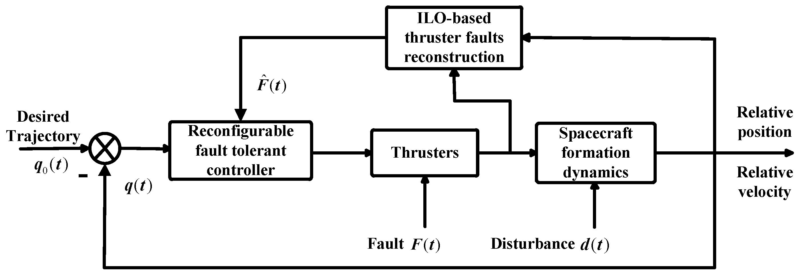
In this section, based on thruster bias faults reconstructed using the designed ILO, an LOF²TC approach was developed for spacecraft formation control systems such that on-orbit desired spacecraft formation configuration could be accurately tracked in the presence of thruster faults, space perturbations, and possible uncertainties. The block diagram of the tracking control system is shown in Figure 2.

4.1. Design of the Learning Output–Feedback Fault-Tolerant Controller

An anticipated nominal formation configuration without any thruster control and space perturbations was assumed as follows,

$$\{\begin{array}{l}{\dot{\mathit{q}}}_0=\mathit{A}{\mathit{q}}_0\\ {\mathit{y}}_0=\mathit{C}{\mathit{q}}_0\end{array}$$

(28)

where ${\mathit{q}}_0$ is the system state of the nominal configuration. By subtracting (3) from (28), a formation configuration that tracked error dynamics could be established as

$$\{\begin{array}{l}{\dot{\mathit{e}}}_{\mathit{q}}=\mathit{A}{\mathit{e}}_{\mathit{q}}-\mathit{B}\mathit{u}-\mathit{E}\mathit{d}(t)-\mathit{H}\mathit{F}(t)\\ {\mathit{e}}_{\mathit{y}}=\mathit{C}{\mathit{e}}_{\mathit{q}}\end{array}$$

(29)

where ${\mathit{e}}_{\mathit{q}}={\mathit{q}}_0(t)-\mathit{q}(t)$ and ${\mathit{e}}_y(t)={\mathit{y}}_0(t)-\mathit{y}(t)$ are the state tracking error and output tracking error, respectively.

In order to track the desired state of the nominal system and maintain the formation configuration in the presence of thruster faults and space perturbation forces, based on fault-reconstructing signals obtained using the aforementioned ILO (5), the learning output–feedback fault-tolerant tracking controller was established as follows,

$${\mathit{u}}_f=\pi (t)\mathit{K}{\mathit{e}}_{\mathit{y}}-{\mathit{B}}^{+}\mathit{E}\mathit{v}(t)-{\mathit{B}}^{+}\mathit{H}\widehat{\mathit{F}}(t)$$

(30)

where $v(t)$ is a jointed compensation term of both space perturbation forces and actuator fault reconstruction errors; $\pi (t)$ is a learning parameter, which was designed to solve the potential uncertainties; ${\mathit{B}}^{+}\mathit{H}\widehat{\mathit{F}}(t)$ represents the fault compensation term; ${\mathit{B}}^{+}$ is a generalized inverse of matrix $\mathit{B}$; $\mathit{K}\in {ℝ}^{3\times 6}$ is the gain matrix that is designed later. In the controller (30), $\pi (t)$ is updated by the following learning algorithm [27],

$$\pi (t)=G_1\mathit{\pi }(t-\tau )+G_2{\mathit{e}}_q^T{(\mathit{K}\mathit{C})}^T(\mathit{K}\mathit{C}){\mathit{e}}_{\mathit{q}}$$

(31)

where $G_1$ and $G_2$ are scalars that are designed later. Learning parameter $v(t)$ was updated by the following learning algorithm,

$$v(t)={\mathit{G}}_{3}v(t-\tau )+G_4\mathit{K}\mathit{C}{\mathit{e}}_{\mathit{q}}(t)$$

(32)

where ${\mathit{G}}_3=diag\left\{g_1,\hspace{0.17em}{g}_2,\hspace{0.17em}{g}_3\right\},\hspace{0.17em}\hspace{0.17em}{g}_i>0$ and $G_4$ is a constant.

By substituting (30) into (29), a closed-loop spacecraft formation tracking error system could be expressed as:

$$\{\begin{array}{l}{\dot{\mathit{e}}}_{\mathit{q}}=(\mathit{A}-\mathit{B}\pi \mathit{K}\mathit{C}){\mathit{e}}_q(t)-\mathit{E}{\mathit{e}}_h(t)\\ {\mathit{e}}_{\mathit{y}}=\mathit{C}{\mathit{e}}_q\end{array}$$

(33)

where ${\mathit{e}}_h(t)=\mathit{h}(t)-v(t)$ and $\mathit{h}(t)=\mathit{d}(t)+{\mathit{e}}_F(t)$ denote synthesized disturbance forces.

4.2. Stability Analysis of the Learning Output–Feedback Fault-Tolerant Controller

To guarantee the stability and convergence of the formation configuration tracking error dynamics system (29) under the controller (30), the stability proof of the closed-loop formation configuration tracking error dynamics (33) is provided in detail.

Theorem 2.

For the formation configuration tracking error dynamics system (29) under controller (30), if there exists positive definite symmetric matrices${\mathit{P}}_1\in {ℝ}^{6\times 6}$,$\mathit{Q}\in {ℝ}^{6\times 6}$,${\mathit{G}}_3\in {ℝ}^{3\times 3}$, matrix$\mathit{K}\in {ℝ}^{3\times 6}$, and a scalar$G_1$such that the following relations hold,

$${\mathit{P}}_1\mathit{A}+{\mathit{A}}^T{\mathit{P}}_1-{\mathit{P}}_1\mathit{B}{\mathit{B}}^T{\mathit{P}}_1=-\mathit{Q}$$

(34)

$$\mathit{K}\mathit{C}={\mathit{B}}^T{\mathit{P}}_1$$

(35)

$$(1+{\mu }_1+{\gamma }_3)G_1^2-1<0$$

(36)

$$(1+{\mu }_1+{\gamma }_2){\mathit{G}}_3^T{\mathit{G}}_3-{\mathit{I}}_3<0$$

(37)

where$G_2=1/l(1+{\mu }_1)$and$G_4=-1/{\beta }_1(1+{\mu }_1)$with${\mu }_1>0$,${\gamma }_2>0$,${\gamma }_3>0$, the closed-loop formation configuration tracking error dynamics (33) is uniformly ultimately bounded.

Proof of Theorem 2.

Define

$$\{\begin{array}{l}{\rho }_1(t)=\mathit{h}(t)-{\mathit{G}}_3\mathit{h}(t-\tau )\\ {\rho }_2(t)=v(t)-{\mathit{G}}_{3}v(t-\tau )\\ {\rho }_3(t)=\Sigma (t)-G_1\Sigma (t-\tau )\\ {\rho }_4(t)=\pi (t)-G_1\pi (t-\tau )\end{array}$$

(38)

where $\mathit{h}(t)$ and $\Sigma (t)$ denote adaptive learning terms of $v(t)$ and $\pi (t)$, respectively.

Then substituting (31) and (32) into (38) yields

$$\{\begin{array}{l}{\rho }_2(t)=G_4\mathit{K}\mathit{C}{\mathit{e}}_q(t)\\ {\rho }_4(t)=G_2{\mathit{e}}_q^T{(\mathit{K}\mathit{C})}^T(\mathit{K}\mathit{C}){\mathit{e}}_{\mathit{q}}(t)\end{array}$$

(39)

Let $e_{\Gamma }(t)=\Sigma (t)-\pi (t)$, it follows from (38) that

$$\{\begin{array}{l}{\mathit{e}}_h(t)={\rho }_1(t)-{\rho }_2(t)+{\mathit{G}}_3{\mathit{e}}_h(t-\tau )\\ e_{\Gamma }(t)={\rho }_3(t)-{\rho }_4(t)+G_1{e}_{\Gamma }(t-\tau )\end{array}$$

(40)

therefore, the new form of $\pi (t)$ can be described by

$$\begin{array}{l}\pi (t)=\Sigma (t)-e_{\Gamma }(t)\\ \hspace{1em}\hspace{0.17em}\hspace{0.17em}\hspace{0.17em}=\Sigma (t)-\left[{\rho }_3(t)-{\rho }_4(t)+G_1{e}_{\Gamma }(t-\tau )\right]\end{array}$$

(41)

Substituting (41) into (33) leads to

$$\begin{array}{l}{\dot{\mathit{e}}}_q(t)=(\mathit{A}-\mathit{B}\pi \mathit{K}\mathit{C}){\mathit{e}}_q(t)+\mathit{B}[G_1{e}_{\Gamma }(t-\tau )+{\rho }_3(t)-{\rho }_4(t)]\mathit{K}\mathit{C}{\mathit{e}}_{\mathit{q}}(t)\\ \hspace{1em}\hspace{1em}\hspace{1em}\hspace{1em}-\mathit{B}[{\mathit{G}}_3{\mathit{e}}_h(t-\tau )+{\rho }_1(t)-{\rho }_2(t)]\end{array}$$

(42)

Considering the following Lyapunov–Krasovski function candidate

$$V(t)={\mathit{e}}_{\mathit{q}}^T{\mathit{P}}_1{\mathit{e}}_{\mathit{q}}+{\beta }_1{\displaystyle {\int }_{t-\tau }^t{\mathit{e}}_h^T}(s){\mathit{e}}_h(s)ds+l{\displaystyle {\int }_{t-\tau }^t{e}_{\Gamma }^T}(s)e_{\Gamma }(s)ds$$

(43)

where ${\beta }_1>0$ and $l>0$, the derivative of the Lyapunov candidate $\dot{V}(t)$ can be derived as

$$\begin{array}{ll}\dot{V}(t)& ={\mathit{e}}_q^T({\mathit{P}}_1\mathit{A}+{\mathit{A}}^T{\mathit{P}}_1-2\Sigma {\mathit{P}}_1\mathit{B}\mathit{K}\mathit{C}){\mathit{e}}_{\mathit{q}}+2{\mathit{e}}_{\mathit{q}}^T{\mathit{P}}_1\mathit{B}[G_1{e}_{\Gamma }(t-\tau )+{\rho }_3(t)-{\rho }_4(t)]\mathit{K}\mathit{C}{\mathit{e}}_q\\ & -2{\mathit{e}}_q^T{\mathit{P}}_1\mathit{B}[{\mathit{G}}_3{\mathit{e}}_h(t-\tau )+{\rho }_1(t)-{\rho }_2(t)]\hspace{1em}+{\beta }_1[-{\mu }_1{\mathit{e}}_h^T(t){\mathit{e}}_h(t)+(1+{\mu }_1){\mathit{e}}_h^T(t){\mathit{e}}_h(t)\\ & -{\mathit{e}}_h^T(t-\tau ){\mathit{e}}_h(t-\tau )]+l[-{\mu }_1{e}_{\Gamma }^T(t)e_{\Gamma }(t)+(1+{\mu }_1)e_{\Gamma }^T(t)e_{\Gamma }(t)\hspace{1em}-e_{\Gamma }^T(t-\tau )e_{\Gamma }(t-\tau )]\end{array}$$

(44)

where ${\mu }_1\ge 0$. Substituting (40) into (44) leads to

$$\begin{array}{l}\dot{V}(t)={\mathit{e}}_q^T({\mathit{P}}_1\mathit{A}+{\mathit{A}}^T{\mathit{P}}_1-2\Sigma {\mathit{P}}_1\mathit{B}\mathit{K}\mathit{C}){\mathit{e}}_q\hspace{1em}+2{\mathit{e}}_q^T{\mathit{P}}_1\mathit{B}[G_1{e}_{\Gamma }(t-\tau )+{\rho }_3(t)-{\rho }_4(t)]\mathit{K}\mathit{C}{\mathit{e}}_{\mathit{q}}(t)\\ \hspace{1em}\hspace{1em}\hspace{0.17em}\hspace{0.17em}-2{\mathit{e}}_{\mathit{q}}^T{\mathit{P}}_1\mathit{B}[{\mathit{G}}_3{\mathit{e}}_h(t-\tau )+{\rho }_1(t)-{\rho }_2(t)]\hspace{1em}-{\beta }_1{\mu }_1{\mathit{e}}_h^T(t){\mathit{e}}_h(t)\hspace{1em}+{\beta }_1(1+{\mu }_1)[{\rho }_1^T(t){\rho }_1(t)\\ \hspace{1em}\hspace{1em}\hspace{0.17em}\hspace{0.17em}+{\rho }_2^T(t){\rho }_2(t)\hspace{1em}+{\mathit{e}}_h^T(t-\tau ){\mathit{G}}_3^T{\mathit{G}}_3{\mathit{e}}_h(t-\tau )+2{\mathit{e}}_h^T(t-\tau ){\mathit{G}}_3^T{\rho }_1(t)-2{\rho }_2^T(t){\mathit{G}}_3{\mathit{e}}_h(t-\tau )\\ \hspace{1em}\hspace{1em}\hspace{0.17em}\hspace{0.17em}-2{\rho }_2^T(t){\rho }_1(t)]\hspace{1em}\hspace{1em}-{\beta }_1{\mathit{e}}_h^T(t-\tau ){\mathit{e}}_h(t-\tau )\hspace{1em}-l{\mu }_1{e}_{\Gamma }^T(t)e_{\Gamma }(t)-l{e}_{\Gamma }^T(t-\tau )e_{\Gamma }(t-\tau )\\ \hspace{1em}\hspace{1em}\hspace{0.17em}\hspace{0.17em}+l(1+{\mu }_1)[e_{\Gamma }^T(t-\tau )G_1^T{G}_1{e}_{\Gamma }(t-\tau )\hspace{1em}+{\rho }_3^T(t){\rho }_3(t)+{\rho }_4^T(t){\rho }_4(t)+2e_{\Gamma }^T(t-\tau )G_1^T{\rho }_3(t)\\ \hspace{1em}\hspace{1em}\hspace{0.17em}\hspace{0.17em}-2{\rho }_4^T(t)G_1{e}_{\Gamma }(t-\tau )-2{\rho }_4^T(t){\rho }_3(t)]\hspace{1em}\end{array}$$

(45)

With the aid of (35) and (39), we have $2{\mathit{e}}_q^T{\mathit{P}}_1\mathit{B}\mathit{K}\mathit{C}{\mathit{e}}_q=2{\rho }_4/G_2$ and $2{\mathit{e}}_q^T{\mathit{P}}_1\mathit{B}=2{\rho }_2^T/G_4$. Then, let $G_2=1/l(1+{\mu }_1)$ and $G_4=-1/{\beta }_1(1+{\mu }_1)$, the above equality can be simplified into the following form

$$\begin{array}{l}\dot{V}(t)\le {\mathit{e}}_q^T({\mathit{P}}_1\mathit{A}+{\mathit{A}}^T{\mathit{P}}_1-2\Sigma {\mathit{P}}_1\mathit{B}\mathit{K}\mathit{C}){\mathit{e}}_q\hspace{1em}-{\beta }_1{\mu }_1{\mathit{e}}_h^T(t){\mathit{e}}_h(t)+{\beta }_1(1+{\mu }_1)[{\rho }_1^T(t){\rho }_1(t)\\ \hspace{1em}\hspace{1em}\hspace{0.17em}\hspace{0.17em}+{\mathit{e}}_h^T(t-\tau ){\mathit{G}}_3^T{\mathit{G}}_3{e}_h(t-\tau )+2{\mathit{e}}_h^T(t-\tau ){\mathit{G}}_3^T{\rho }_1(t)]-{\beta }_1{\mathit{e}}_h^T(t-\tau ){\mathit{e}}_h(t-\tau )\\ \hspace{1em}\hspace{1em}\hspace{0.17em}\hspace{0.17em}\hspace{1em}-{\mu }_{1}l{e}_{\Gamma }^T(t)e_{\Gamma }(t)+l(1+{\mu }_1)[e_{\Gamma }^T(t-\tau )G_1^T{G}_1{e}_{\Gamma }(t-\tau )+{\rho }_3^T(t){\rho }_3(t)\\ \hspace{1em}\hspace{1em}\hspace{0.17em}\hspace{1em}\hspace{0.17em}+2e_{\Gamma }^T(t-\tau )G_1^T{\rho }_3(t)]-l{e}_{\Gamma }^T(t-\tau )e_{\Gamma }(t-\tau )\end{array}$$

(46)

and defining ${\eta }_1=1+{\mu }_1$, we have the following inequalities:

$$\{\begin{array}{l}2{\eta }_1{\mathit{e}}_h^T(t-\tau ){\mathit{G}}_3^T{\rho }_1(t)\le {\gamma }_2{\mathit{e}}_h^T(t-\tau ){\mathit{G}}_3^T{\mathit{G}}_3{\mathit{e}}_h(t-\tau )+\frac{{\eta }_1^2}{{\gamma }_2}{\rho }_1^T(t){\rho }_1(t)\\ 2{\eta }_1{\mathit{e}}_{\Gamma }^T(t-\tau )G_1^T{\rho }_3(t)\le {\gamma }_3{e}_{\Gamma }^T(t-\tau )G_1^T{G}_1{e}_{\Gamma }(t-\tau )+\frac{{\eta }_1^2}{{\gamma }_3}{\rho }_3^T(t){\rho }_3(t)\end{array}$$

(47)

where ${\gamma }_2>0$ and ${\gamma }_3>0$.

Further, with the aid of (47), (46) can be transformed into

$$\begin{array}{l}\dot{V}(t)\le {\mathit{e}}_q^T[{\mathit{P}}_1\mathit{A}+{\mathit{A}}^T{\mathit{P}}_1-2\Sigma {(\mathit{K}\mathit{C})}^T\mathit{K}\mathit{C}]{\mathit{e}}_q\hspace{1em}-{\beta }_1{\mu }_1{\mathit{e}}_h^T(t){\mathit{e}}_h(t)-{\mu }_{1}l{e}_{\Gamma }^T(t)e_{\Gamma }(t)\hspace{0.17em}\\ \hspace{1em}\hspace{1em}\hspace{0.17em}\hspace{0.17em}+{\beta }_1{\mathit{e}}_h^T(t-\tau )[({\eta }_1+{\gamma }_2){\mathit{G}}_3^2-{\mathit{I}}_3]{\mathit{e}}_h(t-\tau )+{\beta }_1({\eta }_1+\frac{{\eta }_1^2}{{\gamma }_2}){\rho }_1^T{\rho }_1\hspace{0.17em}\\ \hspace{1em}\hspace{1em}\hspace{0.17em}\hspace{0.17em}+l{e}_{\Gamma }^T(t-\tau )[({\eta }_1+{\gamma }_3)G_1^2-1]e_{\Gamma }(t-\tau )+l({\eta }_1+\frac{{\eta }_1^2}{{\gamma }_3}){\rho }_3^T{\rho }_3\end{array}$$

(48)

According to (36) and (37), (48) can be further transformed into

$$\begin{array}{l}\dot{V}(t)\le {\mathit{e}}_q^T[{\mathit{P}}_1\mathit{A}+{\mathit{A}}^T{\mathit{P}}_1-2\Sigma {(\mathit{K}\mathit{C})}^T\mathit{K}\mathit{C}]{\mathit{e}}_q-{\beta }_1{\mu }_1{\mathit{e}}_h^T(t){\mathit{e}}_h(t)-{\mu }_{1}l{e}_{\Gamma }^T(t)e_{\Gamma }(t)\hspace{0.17em}\\ \hspace{1em}\hspace{1em}\hspace{0.17em}\hspace{0.17em}+{\beta }_1({\eta }_1+\frac{{\eta }_1^2}{{\gamma }_2}){\rho }_1^T{\rho }_1\hspace{0.17em}+l({\eta }_1+\frac{{\eta }_1^2}{{\gamma }_3}){\rho }_3^T{\rho }_3\end{array}$$

(49)

Based on (37), it follows that

$$\{\begin{array}{l}\Vert {\rho }_1\Vert \le \Vert \mathit{h}(t)\Vert +\Vert {\mathit{G}}_3\Vert ·\Vert \mathit{h}(t-\tau )\Vert \le {\rho }_{1\max }\\ \Vert {\rho }_3\Vert \le \Vert \Sigma (t)\Vert +\Vert G_1\Vert ·\Vert \Sigma (t-\tau )\Vert \le {\rho }_{3\max }\end{array}$$

(50)

Choosing $2{\Sigma }_{min}\ge 1$, and based on the Lyapunov stability theory, it follows from (49) that the global tracking error ${\mathit{e}}_q(t)$, output estimation error ${\mathit{e}}_y(t)$, and compensation error ${\mathit{e}}_h(t)$ are uniformly ultimately bounded.

Furthermore, the design procedure of the learning output–feedback fault-tolerant controller is given as follows:

(1)

Select appropriate positive scalars $l$, ${\beta }_1$, and ${\mu }_1$, then compute parameters $G_2=1/l(1+{\mu }_1)$ and $G_4=-1/{\beta }_1(1+{\mu }_1)$.

(2)

Select appropriate matrix $\mathit{Q}$, then matrices ${\mathit{P}}_1$ and $\mathit{K}$ can be obtained readily by solving (34) and (35).

(3)

Choose small positive scalars ${\gamma }_2$ and ${\gamma }_3$, then compute $G_1$ and ${\mathit{G}}_3$ through solving (36) and (37).

(4)

Choose the appropriate learning interval $\tau$ and design the controller in the form of (30) according to the above gain matrices and parameters.

□

5. Simulation Studies

In this section, a numerical example is provided to illustrate the effectiveness and superiority of the proposed ILO-based thruster fault reconstruction and LOF²TC-based formation maintenance for a satellite formation flying system. The orbital rate was taken as $n=0.0015 \mathrm{rad}/\mathrm{s}$. The space perturbation model borrowed from [12] is given as follows,

$$\mathit{d}(t)=A_0\left[\begin{array}{c}1-1.5\sin (nt)\\ 0.5\sin (2nt)\\ \sin (nt)\end{array}\right]$$

where $A_0=1.2\times {10}^{-3}\mathrm{N}$. Therefore, using (3) it was easy to obtain satellite the formation flying system model with space perturbation and thruster faults.

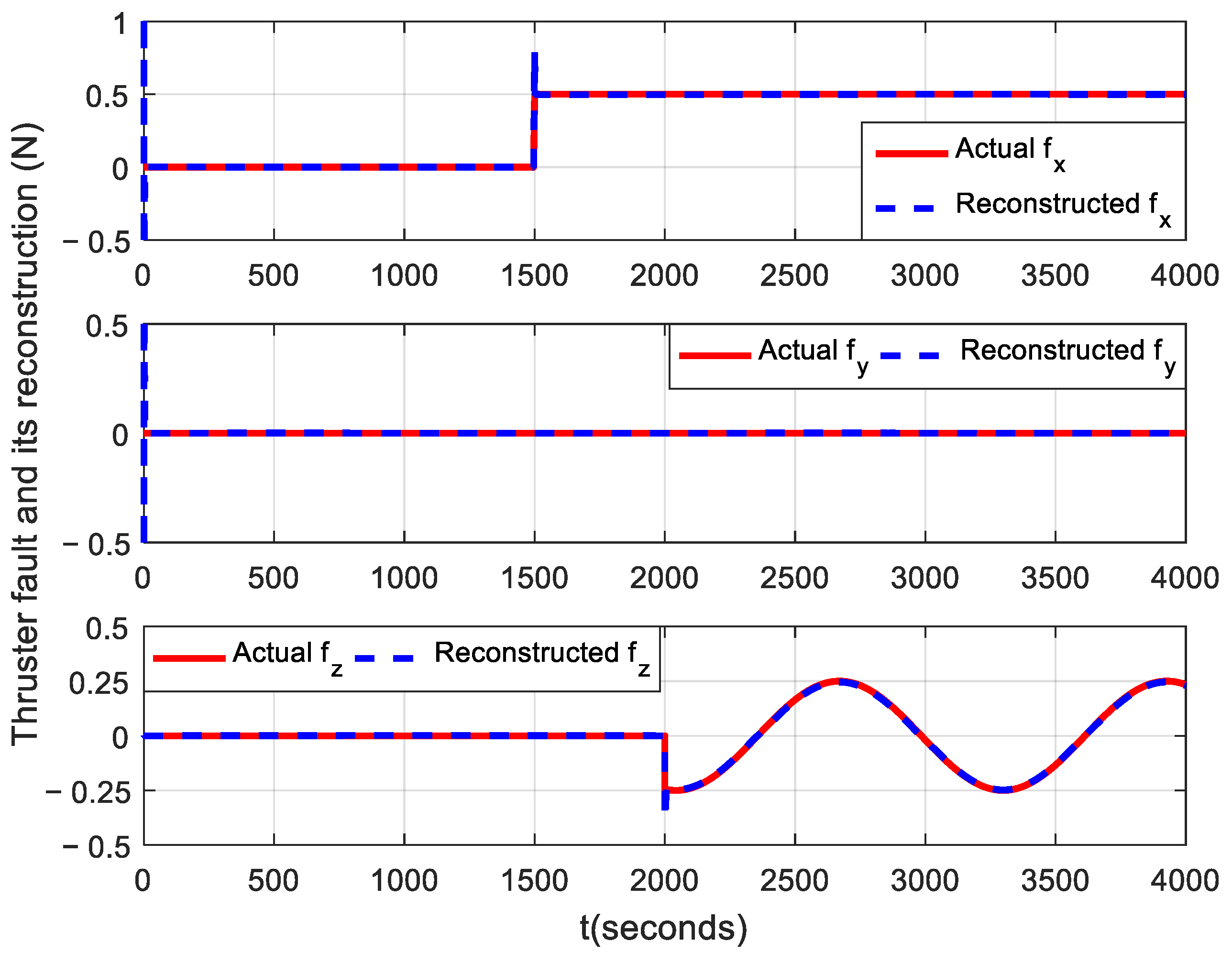
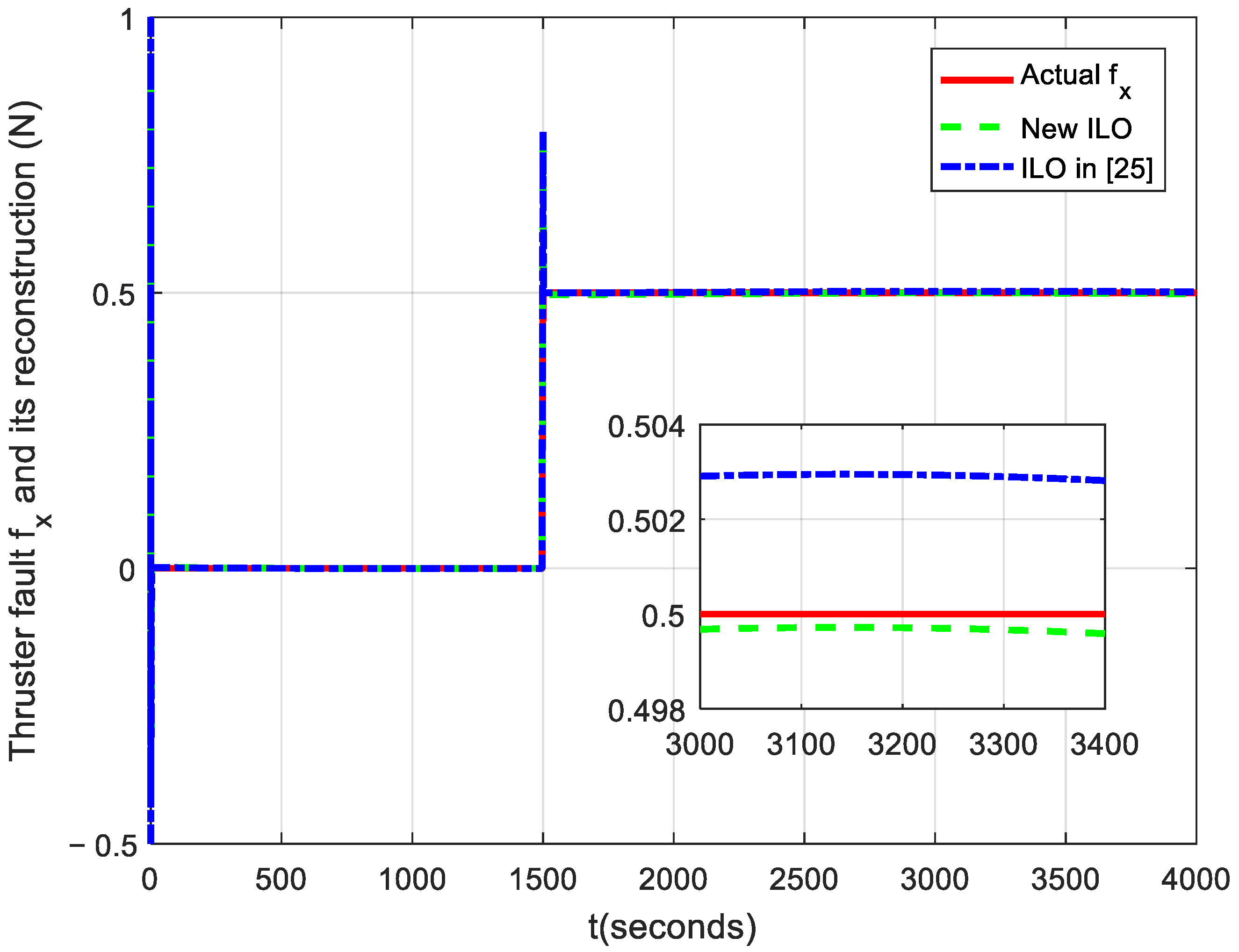
In this work, it was assumed that an abrupt constant fault occurred in the x-axis thruster, a slow time-varying fault occurred in the z-axis thruster, and the thruster in the y-axis was fault free. The fault scenarios were selected as follows:

• The abrupt constant fault in the x-axis thruster:

  $$F_x(t)=\{\begin{array}{l}0\hspace{1em}\hspace{1em}\hspace{0.17em}\hspace{1em}\hspace{0.17em}t\le 1500\mathrm{s}\\ 0.5\hspace{1em}\hspace{1em}\hspace{0.17em}\hspace{0.17em}\hspace{0.17em}t\ge 1500\mathrm{s}\end{array}$$
• Fault-free condition in the y-axis thruster:

  $$F_y(t)=0$$
• The time-varying fault in the z-axis thruster:

  $$F_z(t)=\{\begin{array}{l}0\hspace{1em}\hspace{1em}\hspace{0.17em}\hspace{1em}\hspace{1em}\hspace{1em}\hspace{0.17em}\hspace{0.17em}\hspace{1em}\hspace{1em}\hspace{0.17em}\hspace{0.17em}\hspace{1em}\hspace{1em}\hspace{0.17em}\hspace{0.17em}\hspace{1em}\hspace{1em}\hspace{0.17em}\hspace{0.17em}\hspace{0.17em}t\le 2000\mathrm{s}\\ 0.25\sin (0.05t+\frac{\pi }{4})-0.2e^{-0.1t}\hspace{1em}\hspace{1em}\hspace{0.17em}\hspace{0.17em}\hspace{0.17em}\hspace{1em}t\ge 2000\mathrm{s}\end{array}$$

5.1. ILO-Based Thruster Fault Reconstruction

In the simulation, both the simulation step and the learning interval $\tau$ were set as 0.001 s. Choosing parameters $\mu =0.001$, ${\gamma }_1=0.0193$, and $\beta =1$, one obtained $Q_2=0.999$ and gain matrix ${\mathit{Q}}_1=diag\left\{0.99,0.99,0.99\right\}$. Choosing parameter $\gamma =3.231\times {10}^{-3}$ according to space perturbation $d(t)$ such that the condition in (11) was satisfied. To guarantee good transient performance, all poles of matrix $\mathit{A}-{\mathit{L}}_1\mathit{C}$ could be assigned to stability region $S(-5,2)$ [29]. Solving (8) and (27) with $\lambda ={10}^{-8}$ using the Matlab/LMI toolbox yielded

$${\mathit{L}}_1=\left[\begin{array}{cccccc}4.5471& 0& 0& 1.0000& 0& 0\\ 0& 4.5471& 0& 0& 1.0000& 0\\ 0& 0& 4.5471& 0& 0& 1.0000\\ 0& 0& 0& 4.5470& 0.0030& 0\\ 0& 0& 0& -0.0030& 4.5471& 0\\ 0& 0& 0& 0& 0& 4.5471\end{array}\right]$$

$${\mathit{L}}_2=\left[\begin{array}{cccccc}0& 0& 0& 456.2710& 0& 0\\ 0& 0& 0& 0& 456.2530& 0\\ 0& 0& 0& 0& 0& 456.2642\end{array}\right]$$

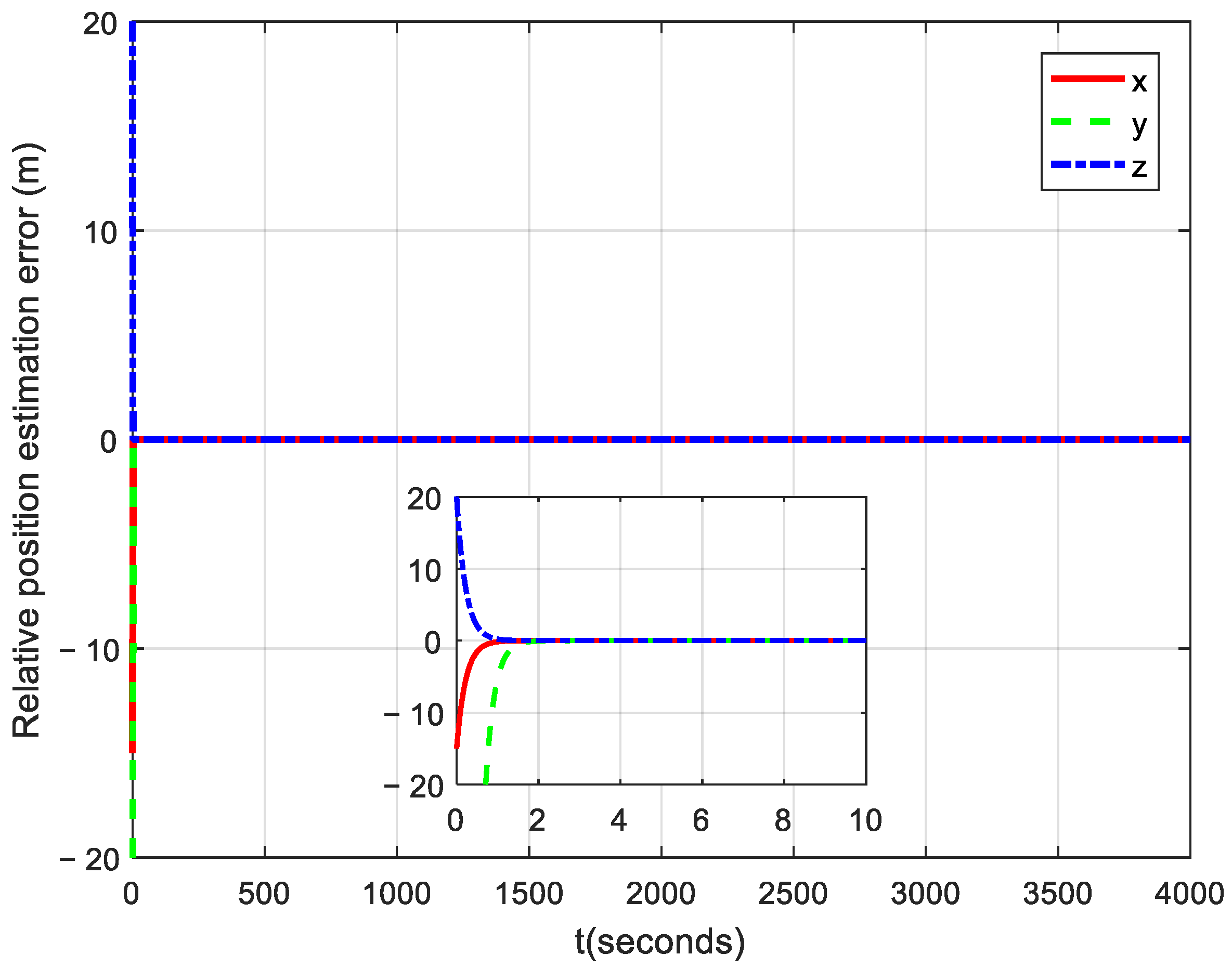
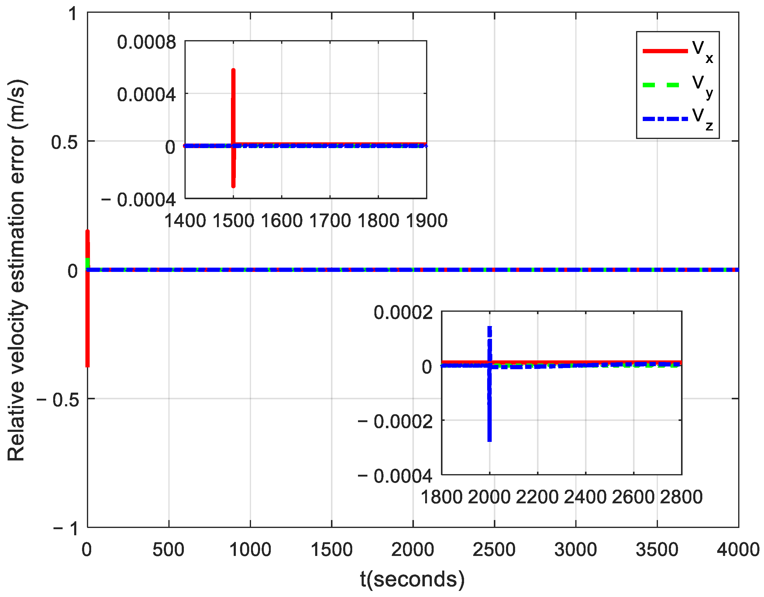
Simulation results on ILO-based thruster fault reconstruction are shown in Figure 3. It was observed that the proposed ILO not only accurately reconstructed the abrupt constant fault in the x-axis thruster, but also had an accurate reconstruction of time-varying faults in the z-axis thruster. In addition, it could be noticed that the reconstruction signal from the proposed ILO converged to the zero region on the y-axis. The estimation errors of relative position and relative velocity are illustrated in Figure 4 and Figure 5. It was clearly demonstrated that the errors could still converge quickly to zero in different fault scenarios. Therefore, the designed ILO could achieve accurate estimations of relative position and relative velocity of the satellite formation flying system.

In order to illustrate the superiority of the proposed robust thruster fault reconstruction approach, a comparison between the proposed ILO and the existing ILO proposed in [25] is provided in the detail. It is worth noting that observer gain matrices and simulation parameters between them were the same. Simulation results on fault reconstruction between them in the x-axis thruster are provided in Figure 6. From these, it could be observed that, compared with the ILO proposed in [25], the new ILO could achieve more accurate fault-reconstructing results in the presence of space perturbations, mainly because the designed ILO had robustness against space perturbations. Therefore, the proposed ILO could achieve accurate fault reconstruction and state estimation simultaneously.

5.2. LOF²TC-Based Formation Configuration Maintenance

Choosing parameters $l=1$, ${\mu }_1=1\times {10}^{-4}$, and ${\beta }_1=1$ yielded $G_2=0.9999$ and $G_4=-0.9999$. $G_1=0.999$ and ${\mathit{G}}_3=\mathrm{diag}\left\{0.999,0.999,0.999\right\}$ were obtained by choosing ${\gamma }_2=0.0009$ and ${\gamma }_3=0.0009$. In this subsection, both the simulation step and the learning interval $\tau$ were taken as 0.001 s, and the initial values of desired state and actual tracking state were chosen to be ${\mathit{q}}_0(0)={[-15, -505, 20, -0.37875, 0.045, 0]}^T$ and $\mathit{q}(0)={[0,\hspace{0.17em}0,\hspace{0.17em}0,\hspace{0.17em}0,\hspace{0.17em}0,\hspace{0.17em}0]}^T$. Solving (34) and (35) yields

$${\mathit{P}}_1=\left[\begin{array}{cccccc}0.0007& 0& 0& 0.0063& 0.0002& 0\\ 0& 0.0007& 0& -0.0002& 0.0063& 0\\ 0& 0& 0.0007& 0& 0& 0.0063\\ 0.0063& -0.0002& 0& 0.1127& 0& 0\\ 0.0002& 0.0063& 0& 0& 0.1126& 0\\ 0& 0& 0.0063& 0& 0& 0.1126\end{array}\right]$$

$$\mathit{K}=\left[\begin{array}{cccccc}0.0063& -0.0002& 0& 0.1127& 0& 0\\ 0.0002& 0.0063& 0& 0& 0.1126& 0\\ 0& 0& 0.0063& 0& 0& 0.1126\end{array}\right]$$

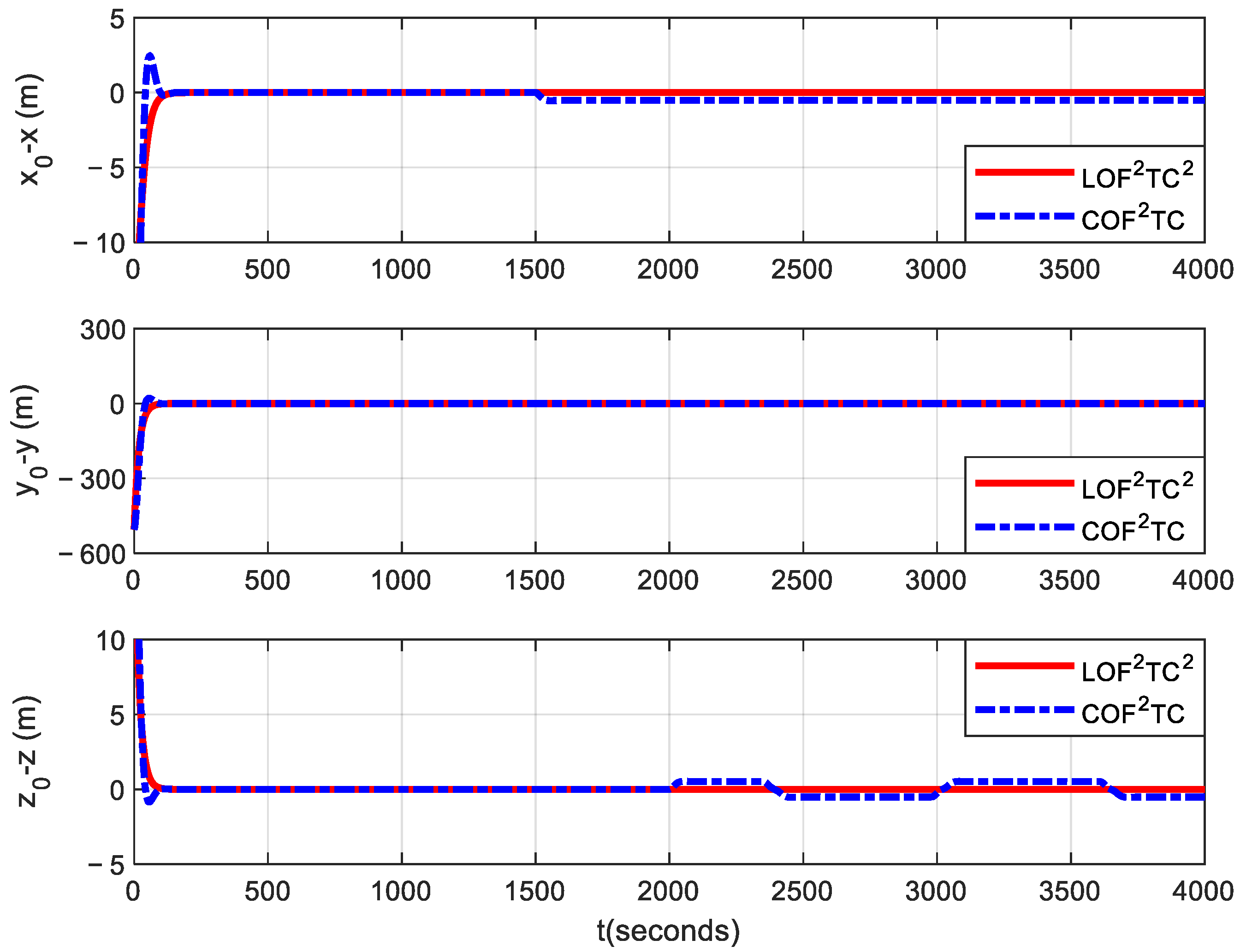
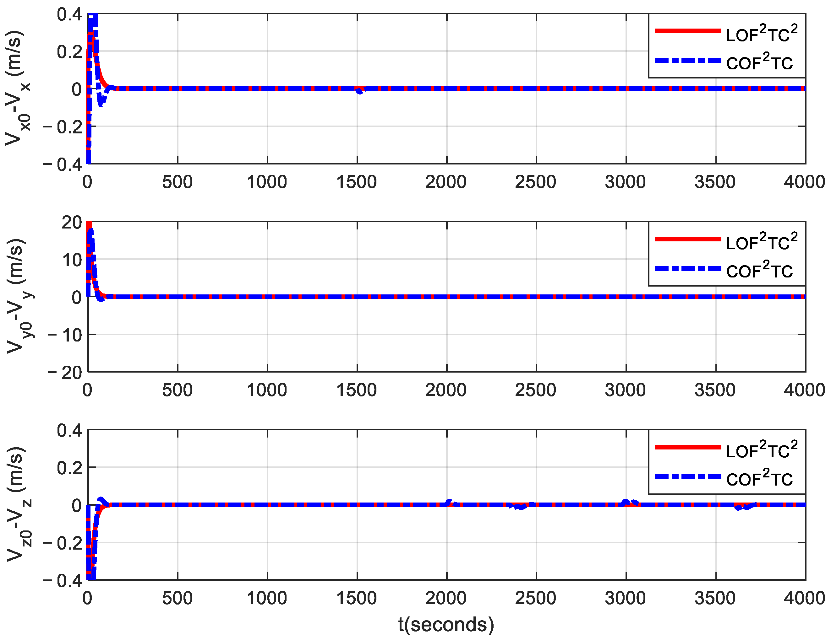
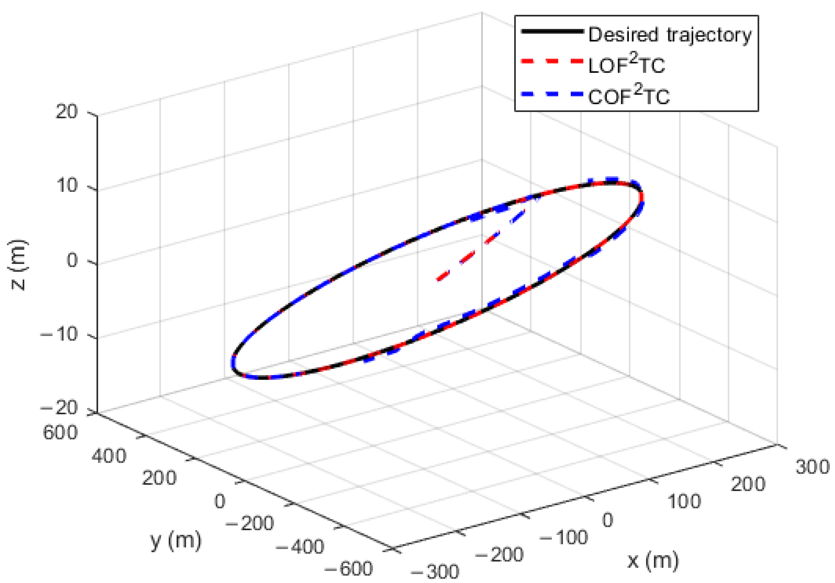
To illustrate the effectiveness and superiority of the LOF²TC-based approach, a simulation comparison between the proposed LOF²TC-based approach and the conventional output–feedback FTC (COF²TC) approach proposed in [30] is provided in detail. Further simulation results are provided in Figure 7, Figure 8, Figure 9 and Figure 10. Figure 7 and Figure 8 demonstrate the curves of relative position tracking error and relative velocity tracking error for satellite formation maintenance control using the proposed LOF²TC approach and the COF²TC approach. From Figure 7, it was also seen that the convergence curve of relative position tracking error deviated from the zero region at 1500 s in the x-axis, and had a fluctuation with small amplitude after 2000 s in the z-axis using the COF²TC approach, while the relative position tracking errors converged to the zero region with higher accuracy under the LOF²TC approach. Figure 9 illustrates the curves of three-dimensional space formation configuration maintenance with space perturbations and thruster faults. From Figure 7, Figure 8 and Figure 9, it could be concluded that the LOF²TC approach could also have better formation maintenance performance than the COF²TC approach.

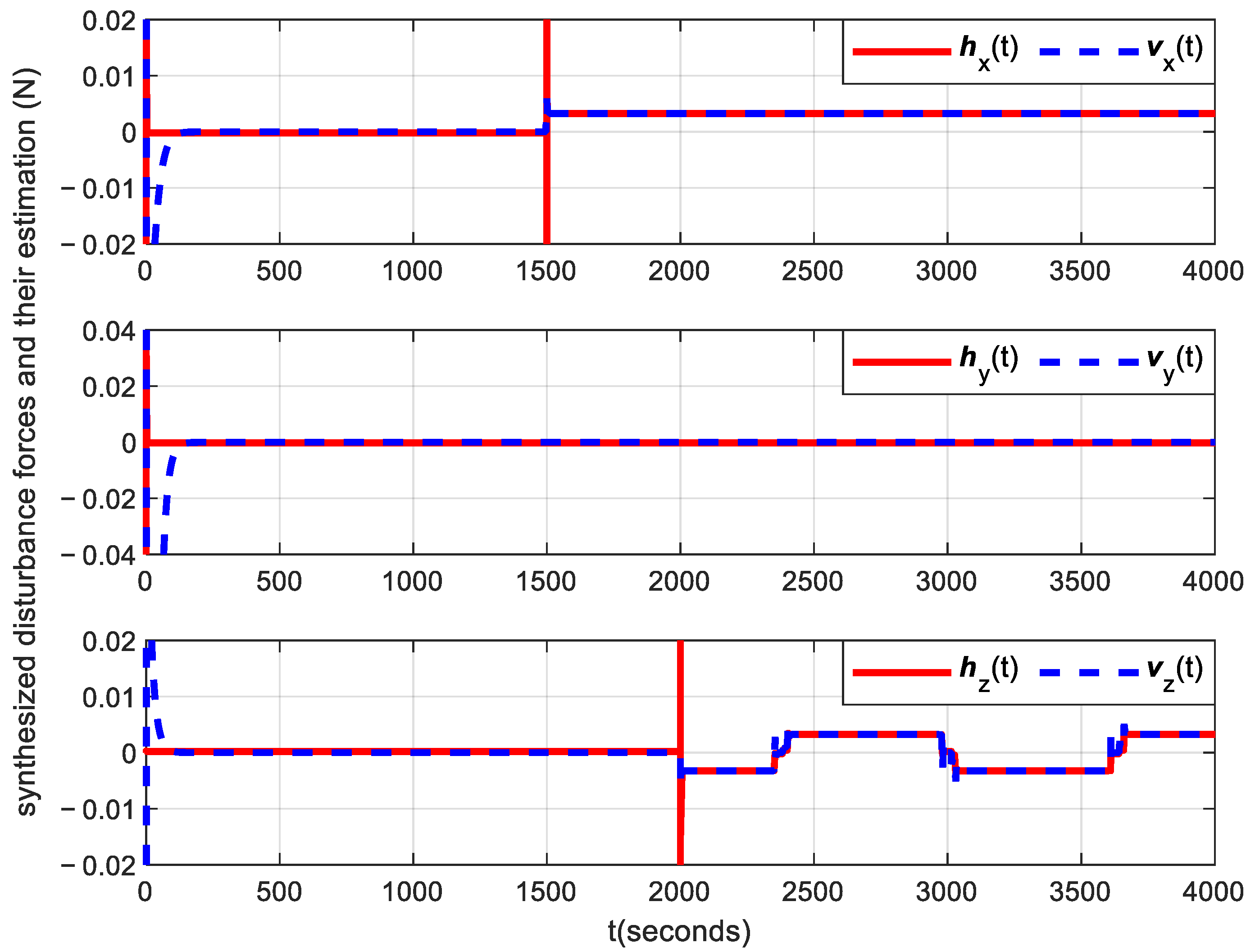
The estimated signal of synthesized disturbance is described in Figure 10, where the iterative learning algorithm could accurately estimate synthesized disturbance; this was the main reason the LOF²TC approach had a better formation maintenance performance than the COF²TC approach. Therefore, based on the designed ILO, the developed LOF²TC approach could achieve spacecraft formation maintenance with high accuracy under the space perturbations and thruster faults.

6. Conclusions

This paper investigated the issues of iterative learning algorithm-based robust thruster fault reconstruction and reconfigurable fault-tolerant control for spacecraft formation flying systems, subject to space perturbations. A novel ILO was developed for robust thruster fault reconstruction. A systematic computation approach of partial ILO gain matrices was provided using LMI optimization techniques. Based on fault-reconstruction signals, an LOF²TC approach was proposed for closed-loop spacecraft formation flying systems such that accurate spacecraft formation configuration maintenance was fulfilled. Finally, through a series of numerical simulations, the effectiveness and superiority of the proposed fault reconstruction and fault-tolerant formation control approaches were verified.

We would like to point out that the research on the proposed method in this paper was based on the linear dynamic model for two spacecrafts. There inevitably existed modeling error when considering the chief spacecraft with the elliptical orbit and long-distance formation mission. Therefore, it is an interesting issue and an extension of the proposed approaches to a more practical nonlinear spacecraft formation flying system, which will be investigated in the near future. In addition, an extension of the proposed approaches to multi-spacecraft formation flying systems is also a meaningful research topic.

References

- Wang, D.; Wu, B.; Chung, E.K.P. Satellite Formation Flying; Springer: Singapore, 2017. [Google Scholar]
- Mathavaraj, S.; Padhi, R. Satellite Formation Flying; Springer: New Delhi, India, 2021. [Google Scholar]
- Alfriend, K.T.; Vadali, S.R.; Gurfil, P.; How, J.P.; Breger, L.S. Spacecraft Formation Flying: Dynamics, Control and Navigation; Elsevier Science & Technology: London, UK, 2009. [Google Scholar]
- Scharf, D.P.; Hadaegh, F.Y.; Ploen, S.R. A survey of spacecraft formation flying guidance and control. Part II: Control. In Proceedings of the 2004 American Control Conference, Boston, MA, USA, 30 June–2 July 2004; Volume 4, pp. 2976–2985. [Google Scholar]
- Liu, Q.P.; Zhang, S.J. A survey on formation control of small satellites. Proc. IEEE 2018, 106, 440–457. [Google Scholar] [CrossRef]
- Marzat, J.; Piet-Lahanier, H.; Damongeot, F.; Walter, E. Model-based fault diagnosis for aerospace systems: A survey. Proc. Inst. Mech. Eng. Part G J. Aerosp. Eng. 2012, 226, 1329–1360. [Google Scholar] [CrossRef] [Green Version]
- Yin, S.; Xiao, B.; Ding, S.X.; Zhou, D.H. A review on recent development of spacecraft attitude fault tolerant control system. IEEE Trans. Ind. Electron. 2016, 63, 3311–3320. [Google Scholar] [CrossRef]
- Barua, A.; Khorasani, K. Hierarchical fault diagnosis and fuzzy rule-based reasoning for satellites formation flight. IEEE Trans. Aerosp. Electron. Syst. 2011, 47, 2435–2456. [Google Scholar] [CrossRef]
- Lian, X.B.; Liu, J.F.; Yuan, L.H.; Cui, N.G. Mixed fault diagnosis scheme for satellite formation. Aircr. Eng. Aerosp. Technol. 2018, 90, 427–434. [Google Scholar] [CrossRef]
- Nemati, F.; Hamami, S.M.S.; Zemouche, A. A nonlinear observer-based approach to fault detection, isolation and estimation for satellite formation flight application. Automatica 2019, 107, 474–482. [Google Scholar] [CrossRef]
- Azizi, S.M.; Khorasani, K. Cooperative state and fault estimation of formation flight of satellites in deep space subject to unreliable information. IFAC Pap. 2019, 52, 206–213. [Google Scholar] [CrossRef]
- Godard, G.; Kumar, K.D. Fault tolerant reconfigurable satellite formations using adaptive variable structure techniques. J. Guid. Control Dyn. 2010, 33, 969–984. [Google Scholar] [CrossRef]
- Cao, L.; Chen, X.Q.; Misra, A.K. Minimum sliding mode error feedback control for fault tolerant reconfigurable satellite formations with J2 perturbations. Acta Astronaut. 2014, 96, 201–216. [Google Scholar] [CrossRef]
- Lee, D.; Kumar, K.D.; Sinha, M. Fault detection and recovery of spacecraft formation flying using nonlinear observer and reconfigurable controller. Acta Astronaut. 2014, 97, 58–72. [Google Scholar] [CrossRef]
- Zhang, Z.J.; Yang, H.; Jiang, B. Decentralised fault-tolerant control of tethered spacecraft formation: An interconnected system approach. IET Control Theory Appl. 2017, 11, 3047–3055. [Google Scholar] [CrossRef]
- Li, P.; Liu, Z.; He, C.; Liu, Q.; Liu, X. Distributed adaptive fault-tolerant control for spacecraft formation with communication delays. IEEE Access 2020, 8, 118653–118663. [Google Scholar] [CrossRef]
- Cheng, P.; Wang, H.; Stojanovic, V.; He, S.; Shi, K.; Luan, X.; Liu, F.; Sun, C. Synchronous fault detection observer for 2-d markov jump systems. IEEE Trans. Cybern. 2021, 1–12. [Google Scholar] [CrossRef]
- Tao, H.F.; LI, X.H.; Paszke, W.; Stojanovic, V.; Yang, H.Z. Robust PD-type iterative learning control for discrete systems with multiple time-delays subjected to polytopic uncertainty and restricted frequency-domain. Multidimens. Syst. Signal Processing 2021, 32, 671–692. [Google Scholar] [CrossRef]
- Jia, Q.X.; Chen, W.; Zhang, Y.C.; Li, H.Y. Fault reconstruction and fault-tolerant control via learning observers in takagi–sugeno fuzzy descriptor systems with time delays. IEEE Trans. Ind. Electron. 2015, 62, 3885–3895. [Google Scholar] [CrossRef]
- Hu, Q.L.; Niu, G.L.; Wang, C.L. Spacecraft attitude fault-tolerant control based on iterative learning observer and control allocation. Aerosp. Sci. Technol. 2018, 75, 245–253. [Google Scholar] [CrossRef]
- Zhang, C.X.; Wang, J.H.; Zhang, D.X.; Shao, X.W. Learning observer based and event-triggered control to spacecraft against actuator faults. Aerosp. Sci. Technol. 2018, 78, 522–530. [Google Scholar] [CrossRef]
- Jia, Q.X.; Li, H.Y.; Chen, X.Q.; Zhang, Y.C. Observer-based reaction wheel fault reconstruction for spacecraft attitude control systems. Aircr. Eng. Aerosp. Technol. 2019, 91, 1268–1277. [Google Scholar] [CrossRef]
- Li, B.; Hu, Q.L.; Ma, G.F.; Yang, Y.S. Fault-tolerant attitude stabilization incorporating closed-loop control allocation under actuator failure. IEEE Trans. Aerosp. Electron. Syst. 2019, 55, 1989–2000. [Google Scholar] [CrossRef]
- Zhu, X.Y.; Chen, J.L.; Zhu, Z.H. Adaptive learning observer for spacecraft attitude control with actuator fault. Aerosp. Sci. Technol. 2021, 108, 106389. [Google Scholar] [CrossRef]
- Jia, Q.X.; Chen, W.; Zhang, Y.C.; Li, H.Y. Fault reconstruction for continuous-time systems via learning observers. Asian J. Control 2016, 18, 549–561. [Google Scholar] [CrossRef]
- Yang, X.B.; Cao, X.B. A new approach to autonomous rendezvous for spacecraft with limited impulsive thrust: Based on switching control strategy. Aerosp. Sci. Technol. 2015, 43, 454–462. [Google Scholar] [CrossRef]
- Peng, Z.H.; Wang, D.; Zhang, H.W. Cooperative tracking and estimation of linear multi-agent systems with a dynamic leader via iterative learning. Int. J. Control 2014, 87, 1163–1171. [Google Scholar] [CrossRef]
- Liu, M.; Shi, P. Sensor fault estimation and tolerant control for Itô stochastic systems with a descriptor sliding mode approach. Automatica 2013, 49, 1242–1250. [Google Scholar] [CrossRef]
- Garcia, G.; Bernussou, J. Pole assignment for uncertain systems in a specified disk by state feedback. IEEE Trans. Autom. Control 1995, 40, 184–190. [Google Scholar] [CrossRef]
- Yang, X.B.; Gao, H.J. Robust reliable control for autonomous spacecraft rendezvous with limited-thrust. Aerosp. Sci. Technol. 2013, 24, 161–168. [Google Scholar] [CrossRef]
Figure 1.
ECI and LVLH coordinate frames for spacecraft formation flying.
Figure 2.
The proposed control framework for maintaining the formation configuration.
Figure 3.
Reconstruction signals from the different fault scenarios.
Figure 4.
Estimation error of relative position using the designed ILO.
Figure 5.
Estimation error of relative velocity using the designed ILO.
Figure 6.
The fault-reconstructing results obtained using the newly designed ILO and the existing ILO.
Figure 7.
Relative position tracking error for formation maintenance.
Figure 8.
Relative velocity tracking error for formation maintenance.
Figure 9.
Three-dimensional tracking trajectory for spacecraft formation configuration maintenance.
Figure 10.
The estimation signal of the synthesized disturbance.
Publisher’s Note: MDPI stays neutral with regard to jurisdictional claims in published maps and institutional affiliations. |
© 2022 by the authors. Licensee MDPI, Basel, Switzerland. This article is an open access article distributed under the terms and conditions of the Creative Commons Attribution (CC BY) license (https://creativecommons.org/licenses/by/4.0/).
Share and Cite
MDPI and ACS Style
Gui, Y.; Jia, Q.; Li, H.; Cheng, Y. Reconfigurable Fault-Tolerant Control for Spacecraft Formation Flying Based on Iterative Learning Algorithms. Appl. Sci. 2022, 12, 2485. https://0-doi-org.brum.beds.ac.uk/10.3390/app12052485
AMA Style
Gui Y, Jia Q, Li H, Cheng Y. Reconfigurable Fault-Tolerant Control for Spacecraft Formation Flying Based on Iterative Learning Algorithms. Applied Sciences. 2022; 12(5):2485. https://0-doi-org.brum.beds.ac.uk/10.3390/app12052485
Chicago/Turabian StyleGui, Yule, Qingxian Jia, Huayi Li, and Yuehua Cheng. 2022. "Reconfigurable Fault-Tolerant Control for Spacecraft Formation Flying Based on Iterative Learning Algorithms" Applied Sciences 12, no. 5: 2485. https://0-doi-org.brum.beds.ac.uk/10.3390/app12052485
Note that from the first issue of 2016, this journal uses article numbers instead of page numbers. See further details here.