
On the Applicability of Approximate Rolling and Sliding Contact Algorithms in Anisothermal Problems with Thermal Softening


Abstract
:1. Introduction
2. Thermoelastoplastic Approximate Algorithms
2.1. Rate-Independent Plasticity for Isotropic Strain Hardening and Thermal Softening
2.2. Approximate Plane-Strain Rolling and Sliding Contact Algorithms
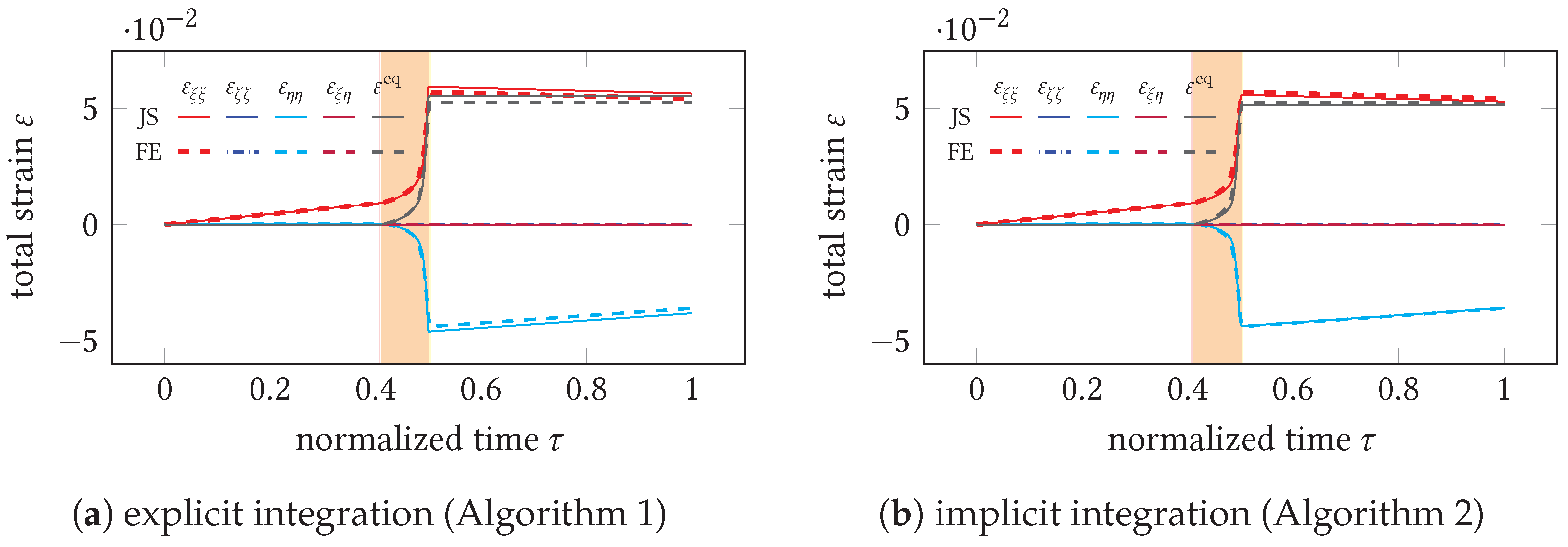
2.3. Numerical Integration Scheme
| Algorithm 1: Explicit integration of stresses and equivalent plastic strain. |
1. Determine and by solving the linear equation system: 2. Update the stresses using the solution from the previous step and as well as . 3. Compute approximations of , , and by Equation (9) with , . 4. Update the equivalent plastic strain, using , and from the previous step: |
| Algorithm 2: Implicit integration of stresses and equivalent plastic strain. |
Compute the root of the following nonlinear equation system via Newton–Raphson iteration: |
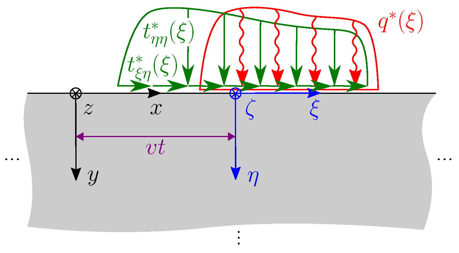
- First, we note that this computational routine needs to be repeated for each individual depth under consideration. However, since there is no direct coupling between the depths, but only indirect coupling through the elastic solution, this may be done in parallel. Generally, since stress and temperature in the elastic solution decay with distance from the loaded strip, a load imbalance should be expected when parallelizing the evaluation of different depths.
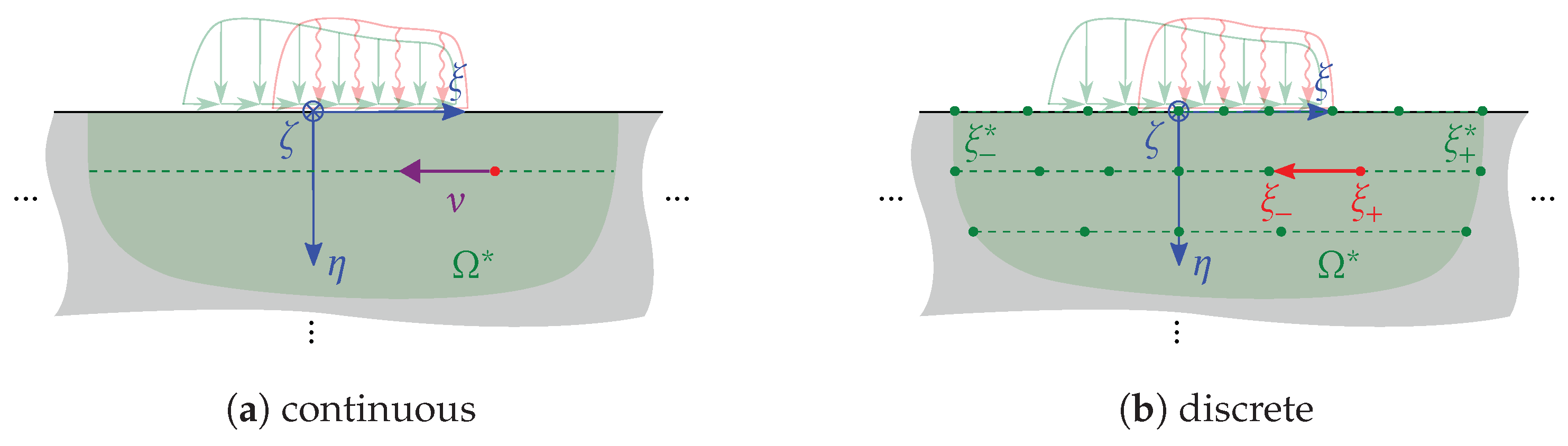
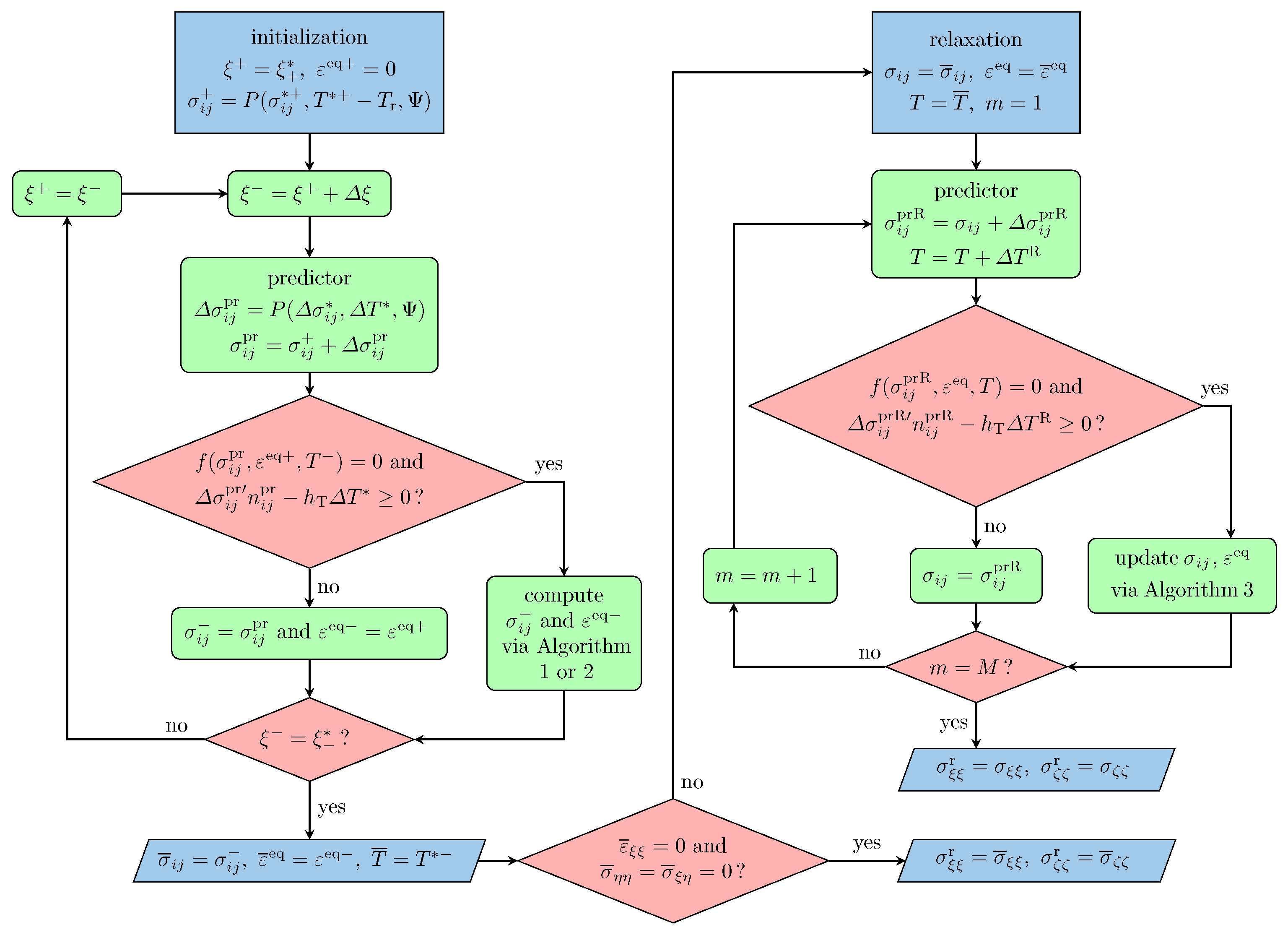
- Initial conditions for the stress and equivalent plastic strain are set at the upmost seen in Figure 2b. For efficiency, shall be set as close as possible to the surface loads while asserting that no plasticity occurs for . Thus, and given that there is no path dependency in the elastic regime, the stress can be initialized by applying the P operator Equation (31), as seen in Figure 3, which effectively yields an equivalent initial state as we would eventually obtain when starting the integration much further away just to ensure initially.
- With the loop construct in the left of Figure 3, we then proceed through the loaded region in (not necessarily constant) increments of , see Figure 2b, thus reconstructing the transient loading history a material point would be subjected to in the elastic moving surface load problem. In doing so, the elastoplastic material response is approximated within the assumptions Equations (11) or (12) by a predictor–corrector approach. Elastoplastic increments are solved using either explicit or implicit integration, as detailed in Algorithms 1 and 2, respectively.
- While the strains generally do not have to be computed explicitly during this first part of the scheme, which is entirely formulated in terms of stresses, all strain components can easily be updated at the end of each increment based on the discretized version of Equation (13). However, doing so is only strictly necessary for , since the only strain component required in the overall scheme is , for which Equation (17) has to be checked prior to potentially invoking the relaxation step.
- Similarly as discussed for the initial condition, it is desirable for efficiency reasons to choose the value of , where the integration is stopped, not too far away from the surface loads. Since the elastic solution does satisfy the Merwin–Johnson conditions Equations (16) and (17) for , which the relaxation eventually enforces, path independency in the elastic regime allows not only a coarsening of the integration step length beyond the plastic zone but also using the relaxation procedure earlier, i.e., starting at larger , to attain the conforming steady state instead of continuing integration toward some excessively far away from the loads. However, this reasoning is only admissible if elastic behavior is guaranteed beyond and likewise during relaxation from onward.
- As indicated above, the Merwin–Johnson conditions are checked for , and that result at from the first step of the scheme. If the check fails, the conditions are enforced by reducing the involved stress and strain components to zero in M increments. Since plasticity may occur during relaxation, M should be sufficiently large to track the associated loading path dependency.
- A very similar predictor–corrector scheme as before is employed during relaxation. However, due to the different set of prescribed stress and strain components, the equations for an elastoplastic relaxation increment differ slightly from the corresponding equations in the previous step of the scheme. Therefore, we collected them in Algorithm 3. Note that we limit the discussion to the case of explicit integration here, since M may conveniently be increased for accuracy, while decreasing during the first step would come at the possibly large additional cost of further evaluations of the elastic input solution.

| Algorithm 3: Integration of stresses and equivalent plastic strain during relaxation. |
1. Determine and by solving the linear equation system
2. Update the stresses using the solution from the previous step and as well as . 3. Update , and by Equation (9) using the updated stress. 4. Update the equivalent plastic strain using , , and from the previous two steps,
|
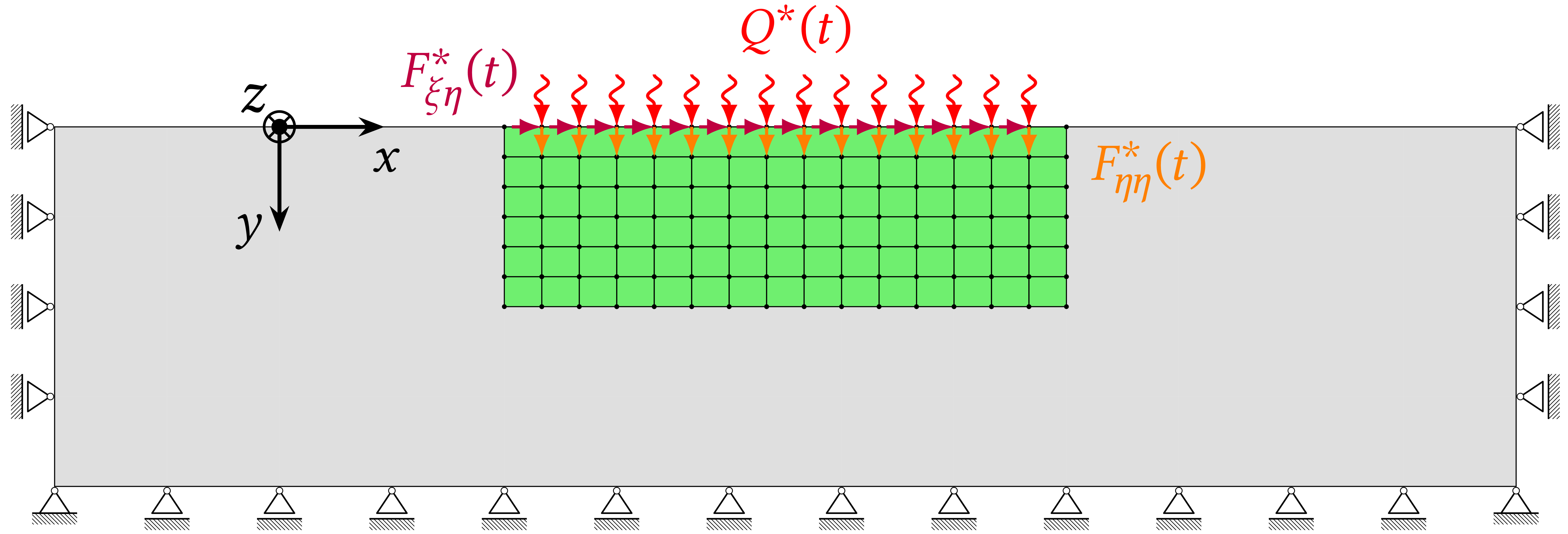
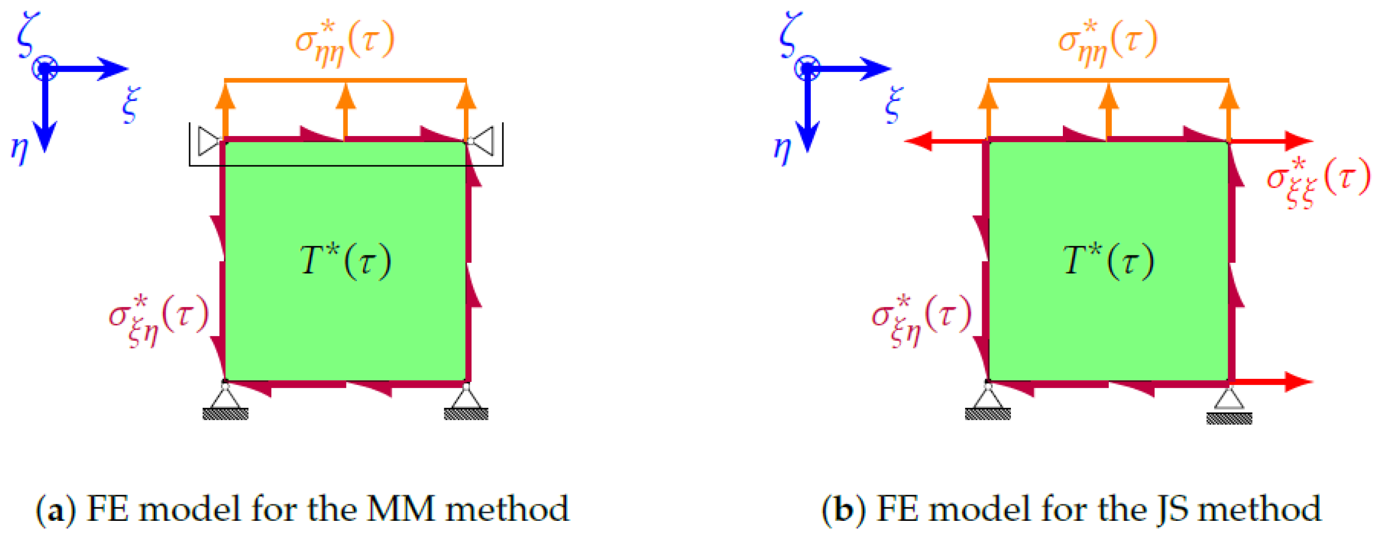
3. Finite Element Modeling
- The elastic solution , , is computed using a transient thermomechanical analysis where thermoelastic material behavior is assumed throughout. The loads are moved over a sufficiently large distance of the model’s surface so that we approximately obtain quasi-stationary fields around the loaded region in a co-moving coordinate system. Then, the analysis is stopped without relieving the mechanical loads or allowing temperature equalization such that we can directly extract the transient loading a material point would be subjected to when passing the loaded region under the preclusion of plasticity.
- To obtain the transient elastoplastic reference solution for material points passing under the surface loads, the above analysis is repeated with thermoelastoplastic material behavior.
- To compute the residual stresses, another thermoelastoplastic analysis is conducted, where the loads are relieved and the temperature is equalized in an additional transient simulation step.

4. Numerical Study and Validation of the Algorithms’ Implementations
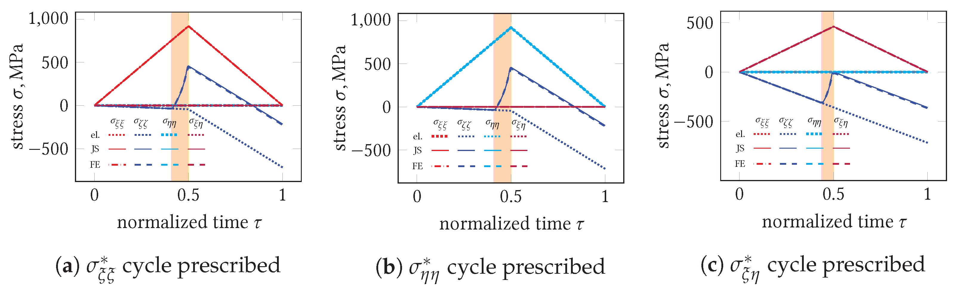
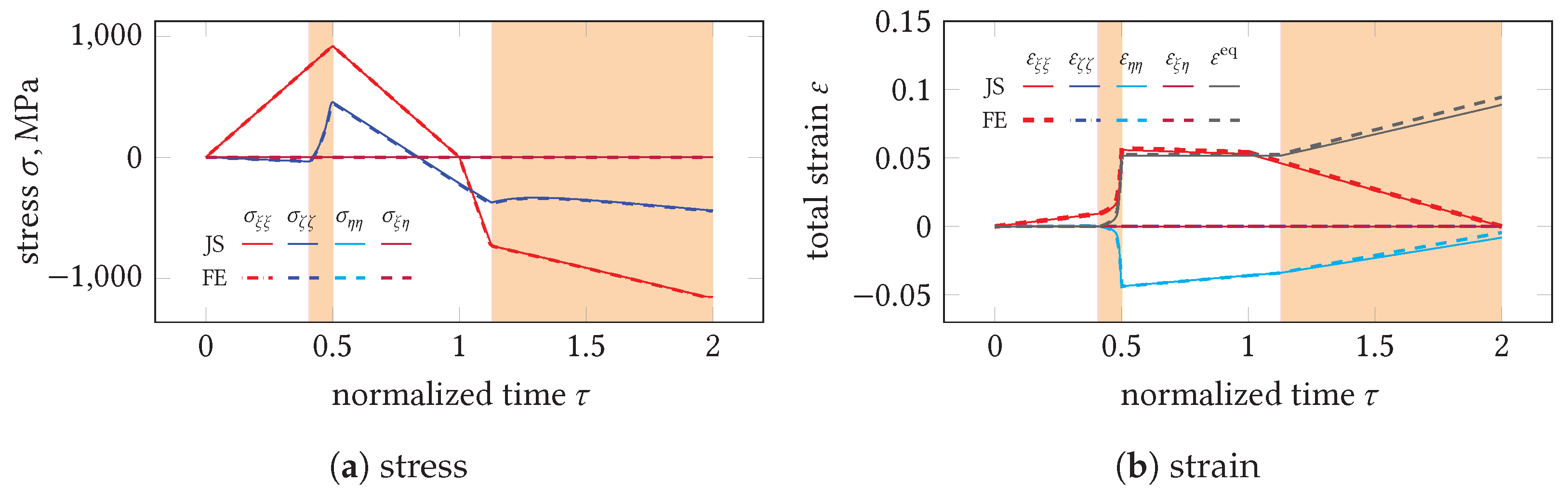
4.1. Validation of the Approximate Algorithms’ Implementation
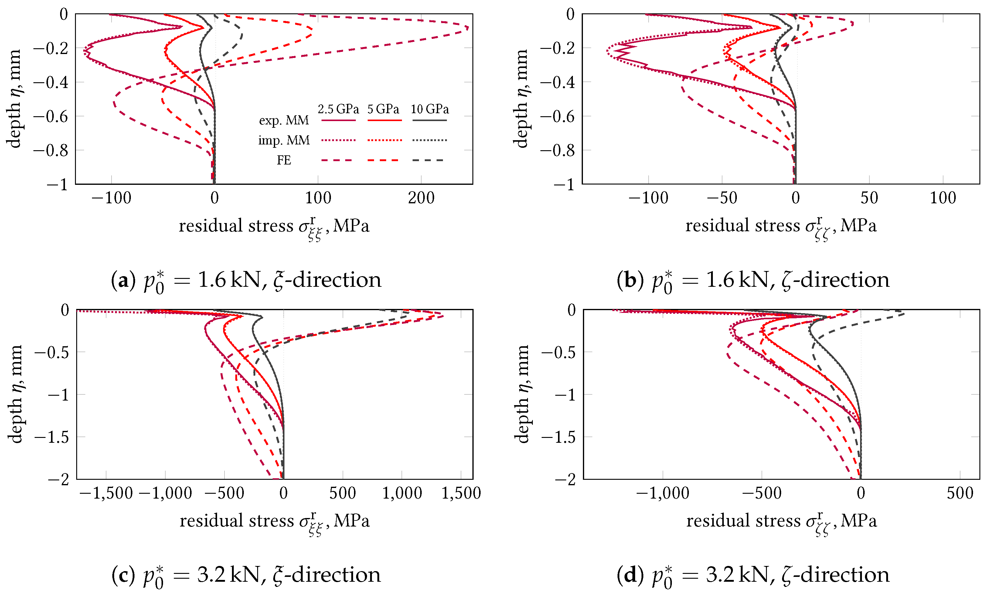
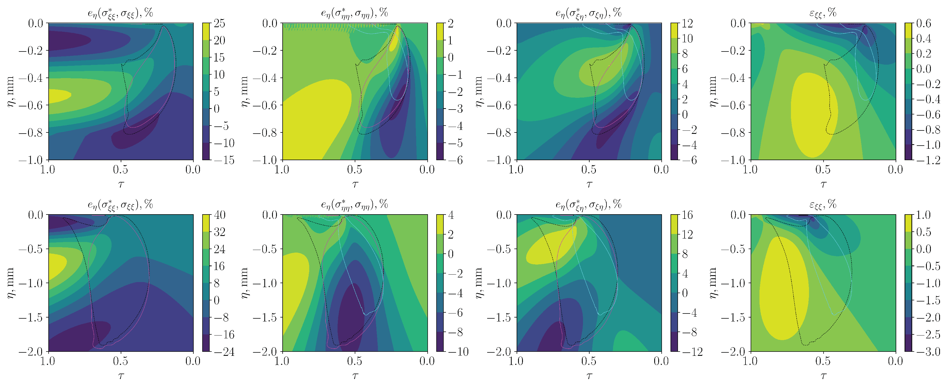
4.2. Analysis of the Approximation Quality for Half-Space Problems
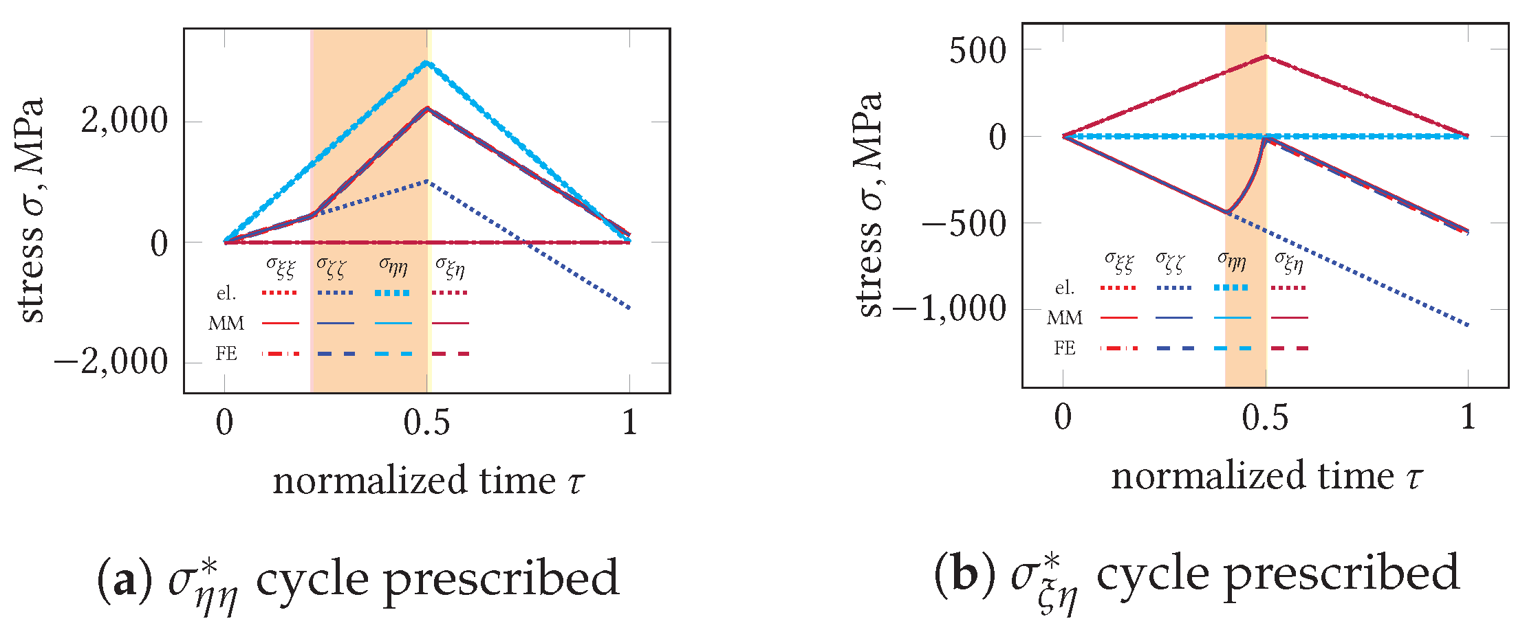
4.2.1. MM Method
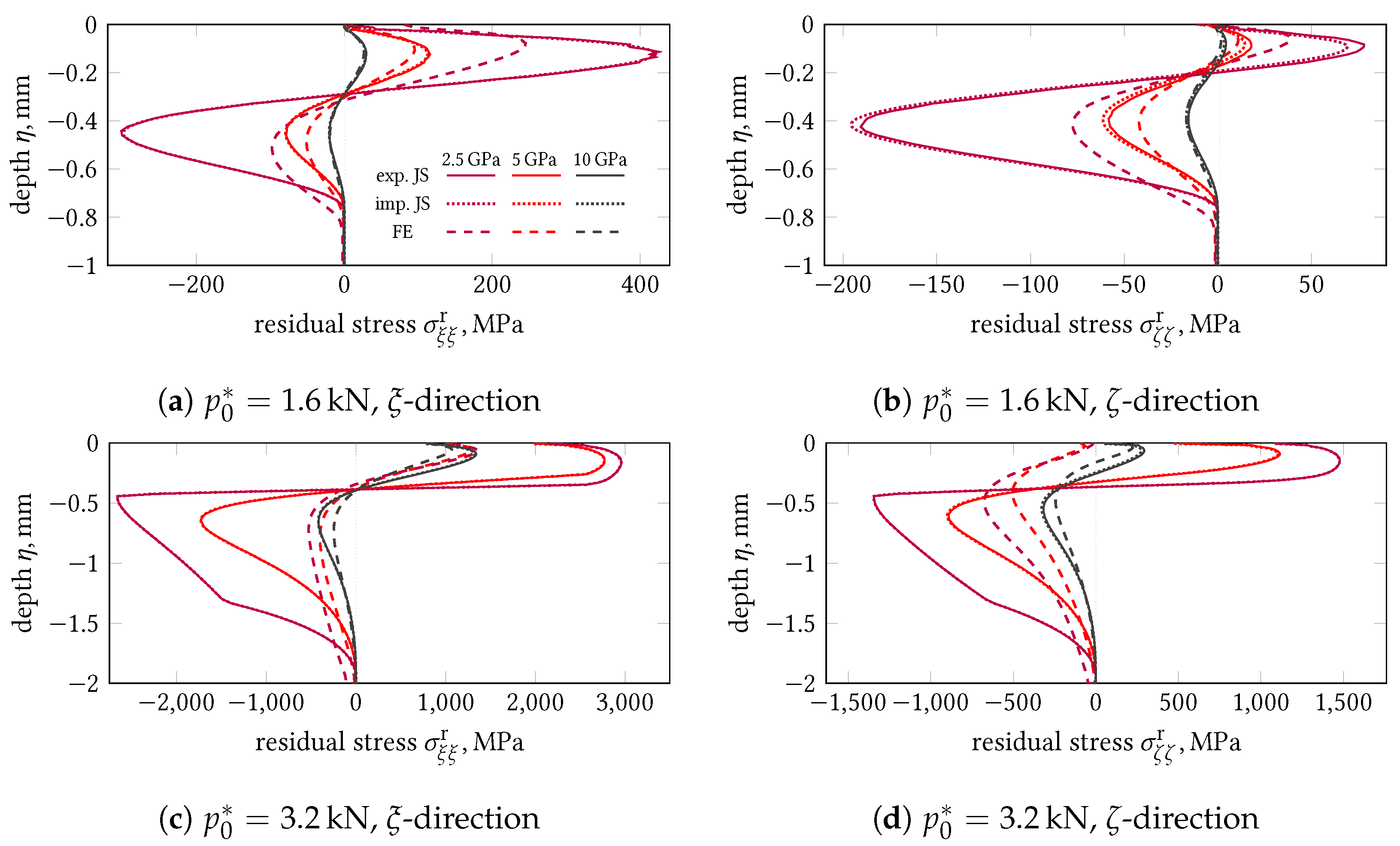
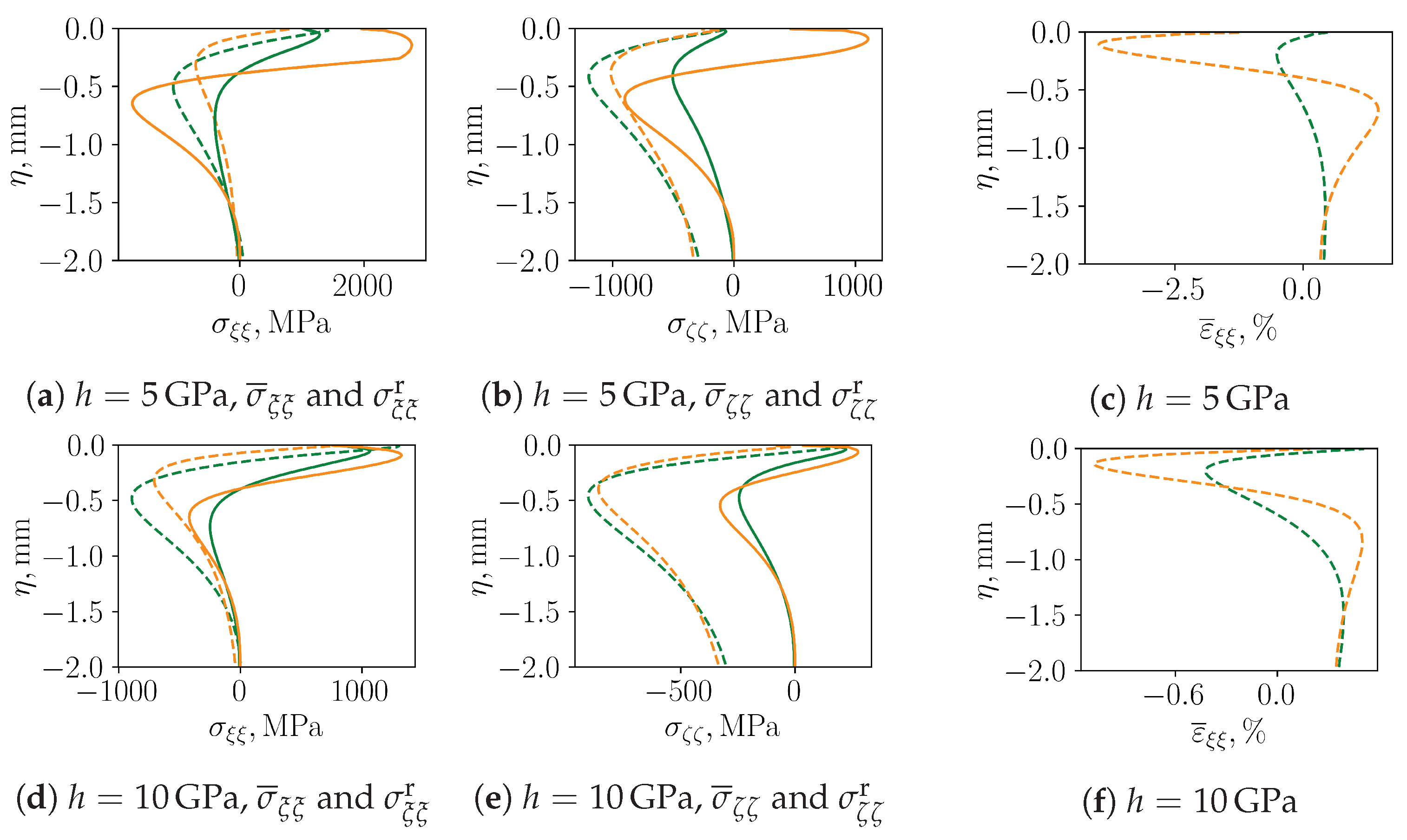
4.2.2. JS Method
5. Discussion
6. Conclusions
- The algorithms are rather sensitive to the hardening slope and require some minimum amount of strain hardening (how much is dependent on the intensity of the prescribed loading) to robustly produce reasonable predictions.
- Due to the strong dependency on the hardening slope, a careful and exact characterization of the strain-hardening behavior is indispensable in order to avoid the possible pitfall of “adjusting” the algorithms to experimental residual stress results by crude constitutive assumptions.
- The MM algorithm does not suit anisothermal problems as studied in this paper due to its inadequate assumption of zero total strain in the moving direction of the surface loads. Specifically, this kinematic constraint inappropriately predetermines the predicted residual stress components to be equal and furthermore introduces increased plastic flow to accommodate the thermal expansion, thus leading to poor approximations especially in the hot surface-near zone.
- In accordance with these limitations of the MM method, we found no obvious incentive to prefer the hybrid algorithm (which effectively reduces to the MM approach for small hardening slopes) over the JS algorithm for the considered type of problem within our investigation. While the hybrid algorithm can be somewhat readjusted to a particular loading and hardening behavior by carefully “tuning” the blending function, doing so requires the knowledge of the correct residual stress distributions beforehand and thus may be impractical when considering a large parameter space as e.g., in prediction or optimization applications.
- The JS method was demonstrated to provide excellent residual stress approximations in anisothermal problems with thermal softening if sufficiently strong strain hardening is present.
- The general approach of uncoupling the problem w.r.t. the depth coordinate , thereby relinquishing kinematic compatibility, and instead relying on the prescribed stress components from the elastic solution to ensure continuity along the depth, appears to be a weak point in all algorithms. Indeed, for larger loads and for smaller hardening slopes, the transient elastoplastic stresses within the loading pass increasingly deviate from the elastic solution, leading to the breakdown of the algorithms with this underlying simplification.
Author Contributions
Funding
Institutional Review Board Statement
Informed Consent Statement
Data Availability Statement
Conflicts of Interest
References
- Jacobus, K.; DeVor, R.E.; Kapoor, S.G. Machining-Induced Residual Stress: Experimentation and Modeling. J. Manuf. Sci. Eng. 1999, 122, 20–31. [Google Scholar] [CrossRef]
- Ulutan, D.; Özel, T. Machining induced surface integrity in titanium and nickel alloys: A review. Int. J. Mach. Tools Manuf. 2011, 51, 250–280. [Google Scholar] [CrossRef]
- Wimmer, M.; Woelfle, C.H.; Krempaszky, C.; Zaeh, M.F. The influences of process parameters on the thermo-mechanical workpiece load and the sub-surface residual stresses during peripheral milling of Ti-6Al-4V. Procedia CIRP 2021, 102, 471–476. [Google Scholar] [CrossRef]
- Wölfle, C.H.; Wimmer, M.; Hameed, M.Z.S.; Krempaszky, C.; Zäh, M.; Werner, E. Towards real-time prediction of residual stresses induced by peripheral milling of Ti–6Al–4V. Contin. Mech. Thermodyn. 2020, 33, 1023–1039. [Google Scholar] [CrossRef]
- Merwin, J.; Johnson, K. An Analysis of Plastic Deformation in Rolling Contact. Proc. Inst. Mech. Eng. Appl. Mech. Group 1963, 177, 676–690. [Google Scholar]
- McDowell, D.; Moyar, G. Effects of non-linear kinematic hardening on plastic deformation and residual stresses in rolling line contact. Wear 1991, 144, 19–37. [Google Scholar] [CrossRef]
- Jiang, Y.; Sehitoglu, H. An Analytical Approach to Elastic-Plastic Stress Analysis of Rolling Contact. ASME J. Tribol. 1994, 116, 577–587. [Google Scholar] [CrossRef]
- McDowell, D. An approximate algorithm for elastic-plastic two-dimensional rolling/sliding contact. Wear 1997, 211, 237–246. [Google Scholar] [CrossRef]
- Ulutan, D.; Alaca, B.E.; Lazoglu, I. Analytical modelling of residual stresses in machining. J. Mater. Process. Technol. 2007, 183, 77–87. [Google Scholar] [CrossRef]
- Liang, S.; Su, J.C. Residual Stress Modeling in Orthogonal Machining. CIRP Ann. 2007, 56, 65–68. [Google Scholar] [CrossRef]
- Zhang, C.; Wang, L.; Meng, W.; Zu, X.; Zhang, Z. A novel analytical modeling for prediction of residual stress induced by thermal-mechanical load during orthogonal machining. Int. J. Adv. Manuf. Technol. 2020, 109, 475–489. [Google Scholar] [CrossRef]
- Weng, J.; Liu, Y.; Zhuang, K.; Xu, D.; M’Saoubi, R.; Hrechuk, A.; Zhou, J. An analytical method for continuously predicting mechanics and residual stress in fillet surface turning. J. Manuf. Process. 2021, 68, 1860–1879. [Google Scholar] [CrossRef]
- Huang, X.; Zhang, X.; Ding, H. An analytical model of residual stress for flank milling of Ti-6Al-4V. Procedia CIRP 2015, 31, 287–292. [Google Scholar] [CrossRef] [Green Version]
- Su, J.C.; Young, K.A.; Ma, K.; Srivatsa, S.; Morehouse, J.B.; Liang, S.Y. Modeling of residual stresses in milling. Int. J. Adv. Manuf. Technol. 2013, 65, 717–733. [Google Scholar] [CrossRef]
- Yue, C.; Hao, X.; Ji, X.; Liu, X.; Liang, S.Y.; Wang, L.; Yan, F. Analytical Prediction of Residual Stress in the Machined Surface during Milling. Metals 2020, 10, 498. [Google Scholar] [CrossRef] [Green Version]
- Fergani, O.; Berto, F.; Welo, T.; Liang, S.Y. Analytical modelling of residual stress in additive manufacturing. Fatigue Fract. Eng. Mater. Struct. 2016, 40, 971–978. [Google Scholar] [CrossRef]
- Mirkoohi, E.; Li, D.; Garmestani, H.; Liang, S.Y. Analytical Modeling of Residual Stress in Laser Powder Bed Fusion Considering Volume Conservation in Plastic Deformation. Modelling 2020, 1, 242–259. [Google Scholar] [CrossRef]
- Bhargava, V.; Hahn, G.T.; Rubin, C.A. An Elastic-Plastic Finite Element Model of Rolling Contact, Part 1: Analysis of Single Contacts. J. Appl. Mech. 1985, 52, 67–74. [Google Scholar] [CrossRef]
- Bhargava, V.; Hahn, G.T.; Rubin, C.A. An Elastic-Plastic Finite Element Model of Rolling Contact, Part 2: Analysis of Repeated Contacts. J. Appl. Mech. 1985, 52, 75–82. [Google Scholar] [CrossRef]
- Xu, B.; Jiang, Y. Elastic-Plastic Finite Element Analysis of Partial Slip Rolling Contact. J. Tribol. 2001, 124, 20–26. [Google Scholar] [CrossRef]
- M’Ewen, E. XLI. Stresses in elastic cylinders in contact along a generatrix (including the effect of tangential friction). Lond. Edinb. Dublin Philos. Mag. J. Sci. 1949, 40, 454–459. [Google Scholar] [CrossRef]
- Carslaw, H.S.; Jaeger, J.C. Conduction of Heat in Solids, 2nd ed.; Clarendon Press: Oxford, UK, 1959. [Google Scholar]
- Zhou, R.; Yang, W. Analytical modeling of residual stress in helical end milling of nickel-aluminum bronze. Int. J. Adv. Manuf. Technol. 2017, 89, 987–996. [Google Scholar] [CrossRef]


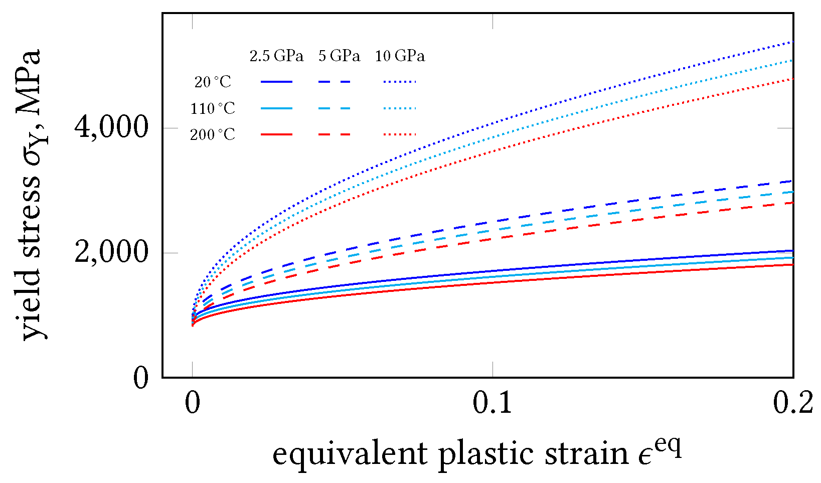
| Symbol | Value | Unit | Description |
|---|---|---|---|
| E | 113.8 | Young’s modulus | |
| 0.342 | Poisson’s ratio | ||
| 9.0 × 10⁻⁶ | K−1 | coefficient of thermal expansion | |
| 920 | initial yield stress | ||
| h | 185 | hardening slope | |
| n | 0.3 | strain-hardening exponent | |
| 20 | transition temperature | ||
| 1650 | melting temperature | ||
| m | 1 | thermal-softening exponent | |
| 4420 | kg m−3 | density | |
| 6.7 | W m−1 K−1 | thermal conductivity | |
| 526.3 | J kg−1 K−1 | specific heat capacity | |
| 20 | ambient temperature |
Publisher’s Note: MDPI stays neutral with regard to jurisdictional claims in published maps and institutional affiliations. |
© 2022 by the authors. Licensee MDPI, Basel, Switzerland. This article is an open access article distributed under the terms and conditions of the Creative Commons Attribution (CC BY) license (https://creativecommons.org/licenses/by/4.0/).
Share and Cite
Wölfle, C.H.; Krempaszky, C.; Werner, E. On the Applicability of Approximate Rolling and Sliding Contact Algorithms in Anisothermal Problems with Thermal Softening. Appl. Sci. 2022, 12, 2549. https://0-doi-org.brum.beds.ac.uk/10.3390/app12052549
Wölfle CH, Krempaszky C, Werner E. On the Applicability of Approximate Rolling and Sliding Contact Algorithms in Anisothermal Problems with Thermal Softening. Applied Sciences. 2022; 12(5):2549. https://0-doi-org.brum.beds.ac.uk/10.3390/app12052549
Chicago/Turabian StyleWölfle, Christoph Hubertus, Christian Krempaszky, and Ewald Werner. 2022. "On the Applicability of Approximate Rolling and Sliding Contact Algorithms in Anisothermal Problems with Thermal Softening" Applied Sciences 12, no. 5: 2549. https://0-doi-org.brum.beds.ac.uk/10.3390/app12052549