Multiclass Skin Lesion Classification Using a Novel Lightweight Deep Learning Framework for Smart Healthcare

Abstract

Skin lesion classification has recently attracted significant attention. Regularly, physicians take much time to analyze the skin lesions because of the high similarity between these skin lesions. An automated classification system using deep learning can assist physicians in detecting the skin lesion type and enhance the patient’s health. The skin lesion classification has become a hot research area with the evolution of deep learning architecture. In this study, we propose a novel method using a new segmentation approach and wide-ShuffleNet for skin lesion classification. First, we calculate the entropy-based weighting and first-order cumulative moment (EW-FCM) of the skin image. These values are used to separate the lesion from the background. Then, we input the segmentation result into a new deep learning structure wide-ShuffleNet and determine the skin lesion type. We evaluated the proposed method on two large datasets: HAM10000 and ISIC2019. Based on our numerical results, EW-FCM and wide-ShuffleNet achieve more accuracy than state-of-the-art approaches. Additionally, the proposed method is superior lightweight and suitable with a small system like a mobile healthcare system.

1. Introduction

Skin lesions, which are irregular skin changes compared to the neighboring tissue, can evolve into skin cancer, one of the most dangerous cancers. There are two main types of skin cancer: nonmelanoma and melanoma. Melanoma lesions are responsible for the significant increase in mortality and morbidity in recent years; they are the most destructive and dangerous among various lesion types [1]. If the physicians detect the lesions earlier, they can increase the curing rate to 90% [2]. Moreover, visual inspection for skin cancer is complex because of high similarity among different skin lesion types (e.g., nonmelanoma and melanoma), leading to misdiagnosis. A solution for healthcare systems [3] and image inspection [4] is using the automatic classification of lesion pictures by machine learning (ML).

Presently, 132,000 melanoma skin lesion cases and approximately three million nonmelanoma skin lesion cases occur yearly in the world. Furthermore, 60,000 people died due to prolonged sun exposure (12,000 nonmelanoma and 48,000 melanoma), according to the World Health Organization. Approximately 80% of skin cancer mortalities occur with melanoma lesions [5]. Besides long sun exposure, a record of sunburn has been linked to the development of skin cancer, especially melanoma. In the beginning grades, patient survival rates can be improved if melanoma is identified correctly [6]. To handle the interobservation differences, technicians are guided to recognize melanoma manually. Consequently, an automatic classification system can enhance the precision and efficiency of the early discovery of this cancer type.

Melanoma is similar to benign moles in their early stages of development; thus, it is not easy to distinguish malignant and benign (even for qualified dermatologists [7]). Several methods have been proposed to solve these problems, including handcrafted and artificial intelligence (AI) approaches.

First, low-level properties, such as border, color, and visual texture features. were used to separate melanoma and nonmelanoma lesions [8]. Celebi et al. [9] used shape, color, and texture features, but experiences with huge observed intraclass similarity led to low results. Segmentation is another approach to drop unwanted features and background, as presented in [10]. Tommasi et al. [10] used a binary mask to segment the images and a support vector machine (SVM) to classify the segmented images. The segmentation process in [11] calculates the thresholding values using Gabor filter masks, which yields poor outcomes.

The second approach is AI, an area with numerous possible utilizations, such as mining, ecology, urban planning. AI is subdivided into ML and deep learning (DL) [12]. ML builds algorithms to identify data and obtain predictions [13,14,15]. DL can study related features of images and extract the features with various architectures. Additionally, DL is highly efficient for big data investigation [16,17,18,19,20,21,22]. One of the DL prototypes is a convolutional neural network (CNN), which has presented an excellent performance in video and images processing with the development of graphics processing unit (GPU) computing systems. CNN is a powerful mechanism for bioimage examination based on a recent study [23,24,25]. Hence, it allows the high potential in melanoma classification [26,27]. Moreover, CNN ensemble approaches have shown success for this classification task [28].

Skin cancer is extremely common, and early detection is crucial. Although computer-aided diagnostic tools have been extensively studied, they still lack clinical practice. ML (and particularly DL) models have demonstrated great promise in skin lesion classification tasks; however, some challenges limit their adoption: data availability for some lesion categories and the requirement of trained professionals handling equipment (e.g., dermatoscopy to collect and annotate the data). Thus, developing powerful but efficient models that can run in decentralized devices (e.g., smartphones) is critical.

Conventional DL methods require high parameters and are not suitable for a portable system. Therefore, creating a framework for a mobile system is a challenging task. Unlike previous methods, we propose a novel approach for skin lesion classification that uses low parameters while keeping high accuracy. The proposed method is appropriate for a portable system like a mobile healthcare system. Our framework combines a novel segmentation technique and a new wide-ShuffleNet to classify skin lesions. The proposed segmentation method increases the segmentation accuracy compared with previous methods and helps the network detect the skin lesion object better boost the classification process.

The contributions of this study are as follows:

• We propose a novel method to segment the skin image using the entropy-based weighting (EW) and first-order cumulative moment (FCM) of the skin image.
• A two-dimensional wide-ShuffleNet network is applied to classify the segmented image after applying EW-FCM. To the best of our knowledge, EW-FCM and wide-ShuffleNet are novel approaches.
• Based on our numerical results on HAM10000 and ISIC2019 datasets, the proposed framework is more efficient and accurate than state-of-the-art methods.

The remainder of the paper is organized as follows. We explore the related works in Section 2. In Section 3, we present the proposed method. Section 4 presents the numerical results and analysis. Finally, Section 5 presents the conclusion and future studies.

2. Related Works

There are two strategies of skin classification: ML and DL methods [29].

2.1. ML Approaches

K-nearest neighbor (KNN) is a supervised ML algorithm used in predictive and forecasting models [30]. The accuracy of the KNN algorithm is considerably good [31]. Sajid et al. [32] proposed another KNN-based automated skin cancer diagnostic system. Their proposed system employed a median filter to remove the image noise using a collection of statistical and textural features. Textural features were extracted from a curvelet domain, whereas statistical features were extracted from lesion images. Furthermore, the proposed framework classified the input images into noncancerous or cancerous. The KNN model requires a long time to perform the output predictions, and it is unsuitable for a big dataset. Moreover, the KNN algorithm operates worst with improper feature information of high dimensional input data, making the algorithm unsuitable for the skin lesion classification [33].

Alam et al. [34] applied SVM to discover eczema. The approach in [35] manipulates several steps: image segmentation, feature determination applying texture-based data, and finally deciding the type of eczema with SVM. Upadhyay et al. [36] extracted orientation histogram, gradient, and location of skin lesion features. These features were fused and classified as malignant or benign using an SVM algorithm. The SVM algorithm is unsuitable for managing the noisy input image [37]. If the number of training samples is less than the number of feature vector parameters, SVM gives a lower performance.

The Bayesian algorithm is another approach used in skin lesion classification with multiple trained skin image databases [38]. Performing the Naïve Bayes algorithm for multiobjective areas is not easy [39]. The decision tree [40] model has been widely used for skin lesion classification, forecast of under limbs lesions, and cervical disease. Arasi et al. [41] presented intelligence techniques, decision tree, and Naïve Bayes to diagnose malignant melanoma. The extracted features are based on principle component analysis and hybrid discrete wavelet transform. These features become the input to different classification methods, such as decision tree and Naïve Bayes, for classifying the lesions as benign or malignant. The decision tree algorithm demands big training data for achieving considerable accuracy. Moreover, the decision tree model requires a large amount of memory and more computational time [42].

2.2. DL Approaches

There are two DL classification strategies for skin classification: non-segmentation [43] and segmentation approaches.

2.2.1. Non-Segmentation DL Approaches

Menegola et al. [44] applied six open datasets for lesion image classification. They used Google Inception-v4 and ResNet-101 architectures to detect seborrheic keratosis, malignant melanoma, and nevus. They also confirmed that combined datasets increase training data and improve classification accuracy. Han et al. [45] introduced Resnet-152 for the lesions image classification. The lesions include squamous cell carcinoma, basal cell carcinoma, actinic keratosis, intraepithelial carcinoma, and malignant melanoma. The factors that reduce the recognition accuracy of skin lesions are image contrast and ethnicity.

Esteva et al. [46] used Inception v3 architecture to classify the lesion into three groups. The method first distinguishes between benign and malignant and then separates seborrheic keratoses and keratinocyte carcinoma types. It also recognizes nevi and malignant melanomas.

Fujisawa et al. [47] classified skin lesions into 21 classes and introduced a four-level lesion identify method. Skin pictures are arranged in four levels using the GoogleLeNet model. Benign and malignant samples are classified first, followed by recognition of melanocytic and epithelial. The method also identified seborrheic keratosis, actinic keratosis, Bowen, and basal cell carcinoma lesions. Zhang et al. [18] inserted an attention layer at the end of ResNet architecture and created new attention residual network. They classified seborrheic keratosis, melanoma, and nevus lesion.

Mahbod et al. [48] introduced a new method to recognize skin lesions using the fine-tuned pretrained network. They first applied AlexNet, VGG16, and ResNet to extract skin image features from the last fully connected layers. Then, they applied SVM to fuse these extracted features. Harangi [49] presented a method that fuses the outcome probabilities of the four CNN models: AlexNet, GoogLeNet, VGGNet, and ResNet. The study proposed the four fusion techniques to identify skin lesions: seborrheic keratosis, melanoma, and nevus. The sum fusion provides better results than other rules (simple majority voting, product fusion, and the maximal probability).

Nyiri and Kiss [50] presented the classification of the dermatological picture using various CNN models, such as VGG19, VGG16, Inception, Xception, DenseNet, and ResNet. They applied these models to extract features of two different inputs: the original skin and segmented images. The proposed method combined these two extracted features to predict skin lesions. Numerical results confirm that ensemble CNN has a better performance than single CNN in skin classification. Consequently, ensemble architecture outperforms individual architecture.

Matsunaga et al. [51] proposed an aggregate DL technique to match three lesion classes: seborrheic keratosis, melanoma, and nevus. They used two binary classifiers on the basis of ResNet-50 architecture. The first classifier distinguishes between melanoma and another lesion. Meanwhile, the second classifier identifies the relationship between seborrheic keratosis and another lesion. The proposed method recognizes the skin lesion images by combining the output probabilities of these two binary classifiers. Li and Shen [52] combined two ResNet architectures and obtained the features at the fully connected layer of each ResNet model. They combined the extracted features to classify skin lesions into seborrheic keratosis, melanoma, and nevus.

2.2.2. Segmentation DL Approaches

Gonzalez–Diaz [53] introduced three architectures to identify skin lesions: segmentation, structure segmentation, and diagnosis stages. First, the skin picture is segmented; then, the output of this stage is used as the input of the structure segmentation stage. Finally, the diagnosis stage links the outputs of the two previous steps and forecasts the skin lesion type. The generation of a labeled training database is the main challenge to creating a structure segmentation network in which each picture has an associated ground truth. This annotation is usually hard to obtain, as it demands a massive effort of the dermatologists to outline the segmentations manually.

The study in [54] employed a DL segmentation model (U-Net) to create a segmented map of the lesion image, cluster sections of abnormal skin, and give the output to a classification network. Meanwhile, Son et al. [54] drew contours of each cluster with the output mask created by U-Net and applied a convex hull algorithm to crop each cluster. Each cluster was applied as input to the EfficientNet to predict the lesion type.

Al-Masni et al. [55] presented an integrated framework that combines skin lesion boundary segmentation and classification steps. First, the study used DL full-resolution convolutional network (FrCN) to segment the skin lesion boundaries. Then, a CNN classifier (ResNet-50, Inception-v3, DenseNet-201, and InceptionResNet-v2) was used to classify the segmented skin lesions. The segmentation step is a crucial prerequisite for skin lesion diagnosis because it extracts principal features of different skin lesions.

Table 1. Datasets of all DL methods.

Methods	Dataset	Number of Images	Number of Classes
Menegola et al. [44]	ISIC 2017	2000	2
Han et al. [45]	Asan	17,125	12
Esteva et al. [46]	DERMOFIT	1300	10
Fujisawa et al. [47]	University of Tsukuba Hospital	6009	21
Mahbod et al. [48]	ISIC 2017	2000	2
Harangi [49]	ISIC 2017	2000	2
Nyiri and Kiss [50]	ISIC 2017	2000	2
Matsunaga et al. [51]	ISIC 2017	2000	2
Li and Shen [52]	ISIC 2017	2000	2
Gonzalez-Diaz [53]	ISIC 2017	2000	2
Unet [54]	DERMNET	15,851	18
Frcn [55]	HAM10000	10,015	7

presents the datasets of all DL methods mentioned in the related work section, including the number of images and classes. Three approaches test with the extensive databases (more than 10,000 images).

Besides DL, other segmentation approaches achieved good results for different fields, such as surface defect detection and mineral separation. Truong et al. [56] presented an automatic thresholding approach that improves Otsu’s method by applying an entropy weighting scheme and overcoming the weakness of Otsu’s technique in defect detection. Zhan et al. [57] presented an ore image segmentation algorithm using a histogram accumulation moment applied to multiscenario ore object recognition. Ore pictures in three separate scenarios are used to demonstrate the effectiveness and accuracy of the proposed approach. It is reasonable to inherit these ideas into bioimage fields.

There are many methods for skin lesion classification in the literature review, including ML and DL frameworks. However, these methods suffer from one of the following drawbacks: (1) missing test results with big data, (2) having insufficiently good performance, and (3) heavy-weight model. In this study, we present a novel approach to overcome these limitations.

3. Methodology

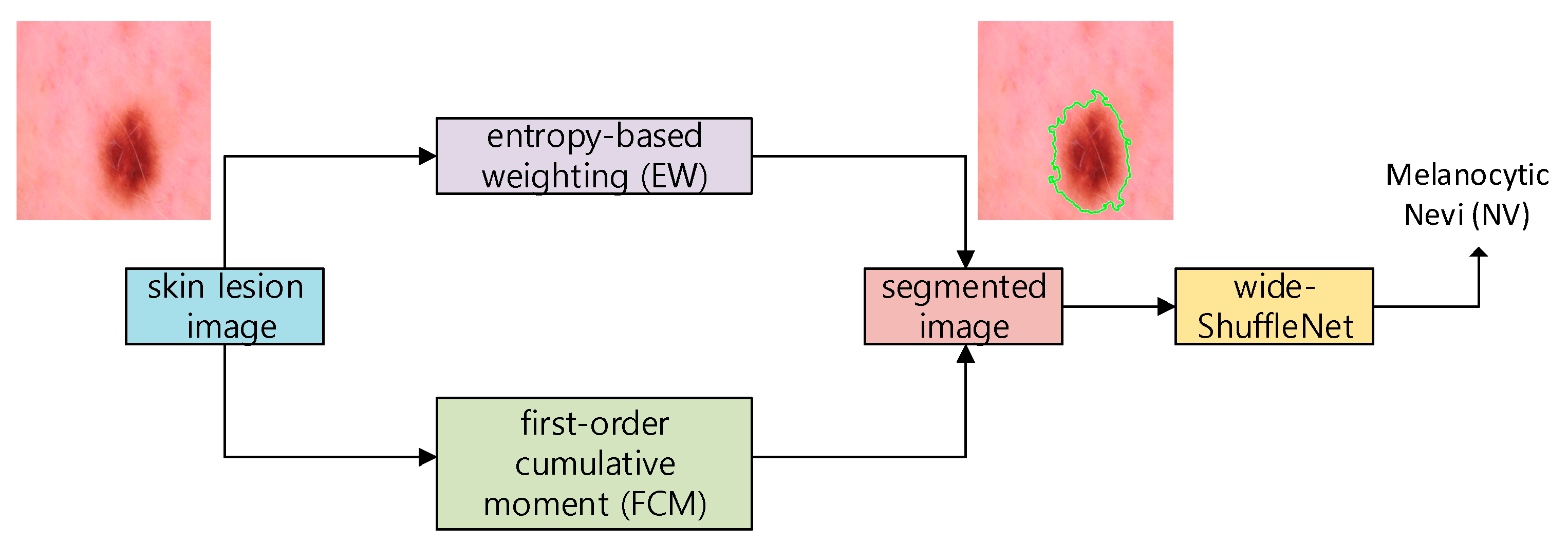
We introduce the novel EW-FCM segmentation technique and a new wide-ShuffleNet for skin lesion classification. The segmentation step helps the network separate between the skin lesion object and background and boosts the recognition process. The segmentation results (full lesion image, including background and foreground) were used as the input of wide-ShuffleNet for feature extraction and classification. Figure 1 shows the structures of the proposed method. We explain how the EW and the first-order cumulative moment were combined to form the new EW-FCM segmentation technique and maintain their good characteristics in Section 3.1. Section 3.2 introduces the wide-ShuffleNet.

3.1. EW-FCM Segmentation Technique

In this section, we first present a short analysis of the Otsu technique. Then, we introduce EW and histogram accumulation moment, including FCM. Finally, the new image threshold technique for image segmentation is presented.

Otsu is one of the most commonly referenced thresholding methods. Let I = g(x,y) be an image with the gray value belonging to the interval [0, 1, …, L − 1]. Assign $n_i$ as the pixel numbers with the gray value $i$ and the total pixel numbers in g(x,y) as $N$. The existence probability of the gray level i is given by

$$P_i=\frac{n_i}{N}.$$

(1)

Assume the threshold $th$ ($0\le th\le L-1$) divides g(x,y) into two classes: background $C_O=\left\{\left(x,y\right)\right|0\le g\left(x,y\right)\le th\}$ and object $C_B=\left\{\left(x,y\right)\right|th+1\le g\left(x,y\right)\le L-1\}$.

The medium gray level of individual class and the probability of category occurrence, respectively, are calculated as follows:

$${\mu }_o\left(th\right)={\displaystyle \sum }_{i=0}^{th}\frac{i{P}_i}{{\omega }_O\left(th\right)}, {\mu }_B\left(th\right)={\displaystyle \sum }_{i=th+1}^{L-1}\frac{i{P}_i}{{\omega }_B\left(th\right)},$$

(2)

where

$${\omega }_O\left(th\right)={\displaystyle \sum }_{i=0}^{th}{P}_i, {\omega }_B\left(th\right)={\displaystyle \sum }_{i=th+1}^{L-1}{P}_i.$$

(3)

In Otsu’s technique, the resulting threshold performance is measured by analyzing the difference between the background and foreground. The optimal threshold $t{h}^{\ast }$ when applying this criterion must maximize between-class variance as follows:

$$\begin{gathered} t{h}^{\ast }=argmax\left\{{\omega }_O\left(th\right){\mu }_O^2\left(th\right)+{\omega }_B\left(th\right){\mu }_B^2\left(th\right)\right\}. \\ 0\le th\le L-1 \end{gathered}$$

(4)

The basic idea to improve Otsu’s technique is the addition of a weight W to the objective function in Equation (4) to regulate the output threshold, given as follows:

$$\begin{gathered} t{h}^{\ast }=argmax\left\{W\left({\omega }_O\left(th\right){\mu }_O^2\left(th\right)+{\omega }_B\left(th\right){\mu }_B^2\left(th\right)\right)\right\}. \\ 0\le th\le L-1 \end{gathered}$$

(5)

Image entropy describes the properties of an image; it is a mathematical measure of randomness. Images with low entropy values possess minimal information and hold many pixels with similar intensity values. An image with zero entropy means that all pixels hold the same gray value. Reference [56] suggested an EW scheme by substituting weight W with the entropy objective function $\psi$(th) in Equation (5) to create a new objective function

$$\begin{gathered} t{h}^{\ast }=argmax\left\{\psi \left(th\right)\left({\omega }_O\left(th\right){\mu }_O^2\left(th\right)+{\omega }_B\left(th\right){\mu }_B^2\left(th\right)\right)\right\}. \\ 0\le th\le L-1 \end{gathered}$$

(6)

The entropy objective function is defined as follows:

$$\psi \left(th\right)=ln({\omega }_O\left(th\right){\omega }_B\left(th\right))+\frac{H_{th}}{{\omega }_O\left(th\right)}+\frac{H_n}{{\omega }_B\left(th\right)},$$

(7)

where

$$H_{th}=-{\displaystyle \sum }_{i=0}^{th}{P}_i\ln \left(P_i\right), H_n=-{\displaystyle \sum }_{i=0}^{L-1}{P}_i\ln \left(P_i\right).$$

(8)

Next, we discuss the first order of the cumulative moment. Let $M_O\left(th\right)$ denotes the FCM of the gray histogram, which is the mean gray value from 0 to $th$ given by

$$M_O\left(th\right)={\displaystyle \sum }_{i=0}^{th}i{P}_i.$$

(9)

The mean gray of the entire image is $M_T$, defined by

$$M_T={\displaystyle \sum }_{i=0}^{L-1}i{P}_i.$$

(10)

The FCM $M_T$ helps the optimal threshold avoid dropping into the local optimum [57].

We combine the EW $\psi$(th) and FCM to obtain the optimal threshold and create a new objective function for image segmentation as follows:

$$\begin{gathered} t{h}^{\ast }=argmax\left\{\psi \left(th\right)\left(M_T\right)\right\}. \\ 0\le th\le L-1 \end{gathered}$$

(11)

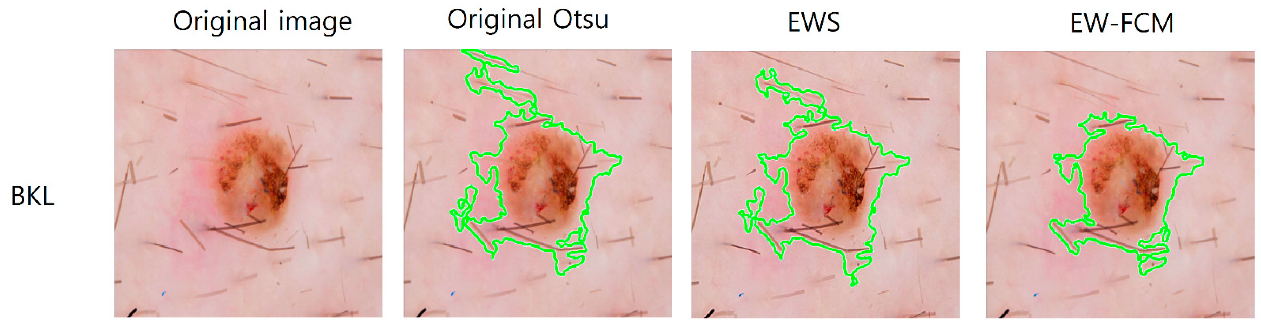
We adopt the segmentation process in reference [58], including texture filtering, threshold and binarize, and plot the boundaries. Zade [58] uses the Otsu method to calculate the threshold; meanwhile, our framework uses the new objective function in Equation (11) to determine the threshold. Our objective function provides a better segmentation technique due to the reservation of all properties of EW-FCM. Figure 2 shows the segmentation results of the original Otsu technique, EW scheme [56], and the proposed EW-FCM segmentation method. As seen in Figure 2, the proposed EW-FCM approach provides better segmentation accuracy than the original Otsu and EW scheme EWS.

3.2. Wide-ShuffleNet

We provide a brief analysis of ShuffleNet inventing for portable devices. Several terms are reviewed, including efficient model designs, group convolution, channel shuffle for group convolutions, and ShuffleNet unit. We also introduce a new variant of ShuffleNet, called wide-ShuffleNet, that has been developed for skin classification.

Efficient model designs: Recently, efficient model designs played an essential role in achieving DL networks in many computer vision tasks [59,60,61]. The growing demand for streaming high-quality DL architectures on embedded systems boosts the research of effective model designs [62]. For instance, instead of assembling convolution layers, GoogLeNet [63] expands the network depth with sufficient lower complexity. ResNet in [64,65] achieves remarkable performance using the effective bottleneck architecture. SqueezeNet [66] preserves accuracy; however, it decreases computation and parameters significantly.

Group convolution: AlexNet [59] is the first model using the idea of group convolution and spreading the network across two GPUs, and ResNeXt [67] confirms the efficacy of group convolution. MobileNet [68] applies the depthwise separable convolution (DWConv) and achieves the best results between lightweight networks. ShuffleNet performs DWConv and group convolution (GConv) in a new style.

Channel shuffle operation: In the early studies on efficient network layout, the operation of channel shuffle is seldom noticed. Lately, another study [69] applied this concept for a two-stage convolution. However, the study [69] did not examine the efficacy of channel shuffle and its application in light network layout.

Channel shuffle for group convolutions: New DL architectures [63,64,65] consist of duplicated structure blocks with identical designs. Among these architectures, ResNeXt [67] and Xception [70] offer an effective GConv or DWConv toward the structure blocks to discover an outstanding trade-off among computational cost and representation capacity. However, both architectures do not use pointwise convolutions [68] (or one-by-one convolutions), which require significant complexity. Increasing the number of one-by-one convolutions, we must restrict the number of channels to meet the complexity constraint in a small network. One possible approach is using the channel links with GConv on the one-by-one layers to handle the limitation. GConv remarkably decreases computation cost by assuring that individual convolution runs on the relative input channel group.

ShuffleNet unit was invented for the light model, benefiting from channel shuffle functioning. ShuffleNet unit gets the ideal from bottleneck unit [64] (see Figure 2a in reference [61]). Building a ShuffleNet unit, the first one-by-one layer in the bottleneck unit is replaced by pointwise GConv accompanied by a channel shuffle functioning (see Figure 2b in reference [61]). The second pointwise GConv retrieves the dimension of the channel to match with the shortcut pathway.

There are two types of ShuffleNet units: nonstride and stride. Two modifications are made to create ShuffleNet with stride (see Figure 2c in reference [61]). First, a three-by-three average pooling is added to the shortcut path. Then, the elementwise addition is altered by channel concatenation, and it is simple to expand the channel dimension with a small additional computational cost. The ShuffleNet model is formed by the ShuffleNet units. The ShuffleNet architecture is made by stacking ShuffleNet units together and classified into three stages. The first block in every stage is implemented with a stride equal to two. Other parameters in the same stage stay identical, and the number of output channels doubled for the following stage.

The proposed wide-ShuffleNet develops from ShuffleNet units and the idea of skip connections. Now, we explore the skip connections. He et al. [64] introduced skip connections that bypass one or many layers (see Figure 2 in reference [64]). Skip connections create the fundamental unit of the residual network, which is considered a residual module [71]. It maintains the feature data over all layers, having longer networks while preserving low parameter numbers. Alternately of getting a desired mapping (indicated as H(x)), the network with skip connection gets a residual mapping (indicated as F(x) + x, with F(x) = H(x) − x). Skip connections make identity mapping and add the result to the output of the two convolutional layers (see Figure 2 in reference [64]).

Next, we apply the long variant of the skip connections to extend the width of the DL architecture. An architecture with a long residual connection converges more quickly and offers excellent performance (see reference [72]). A long residual connection helps the network increase the accuracy as it enhances reused features through the entire network. It also helps the network to get the detailed and general characteristics of objects. A one-by-one convolution layer is inserted in the shortcut connection to create a long residual connection between different sized layers, making the size of two inputs of the additional layer equal.

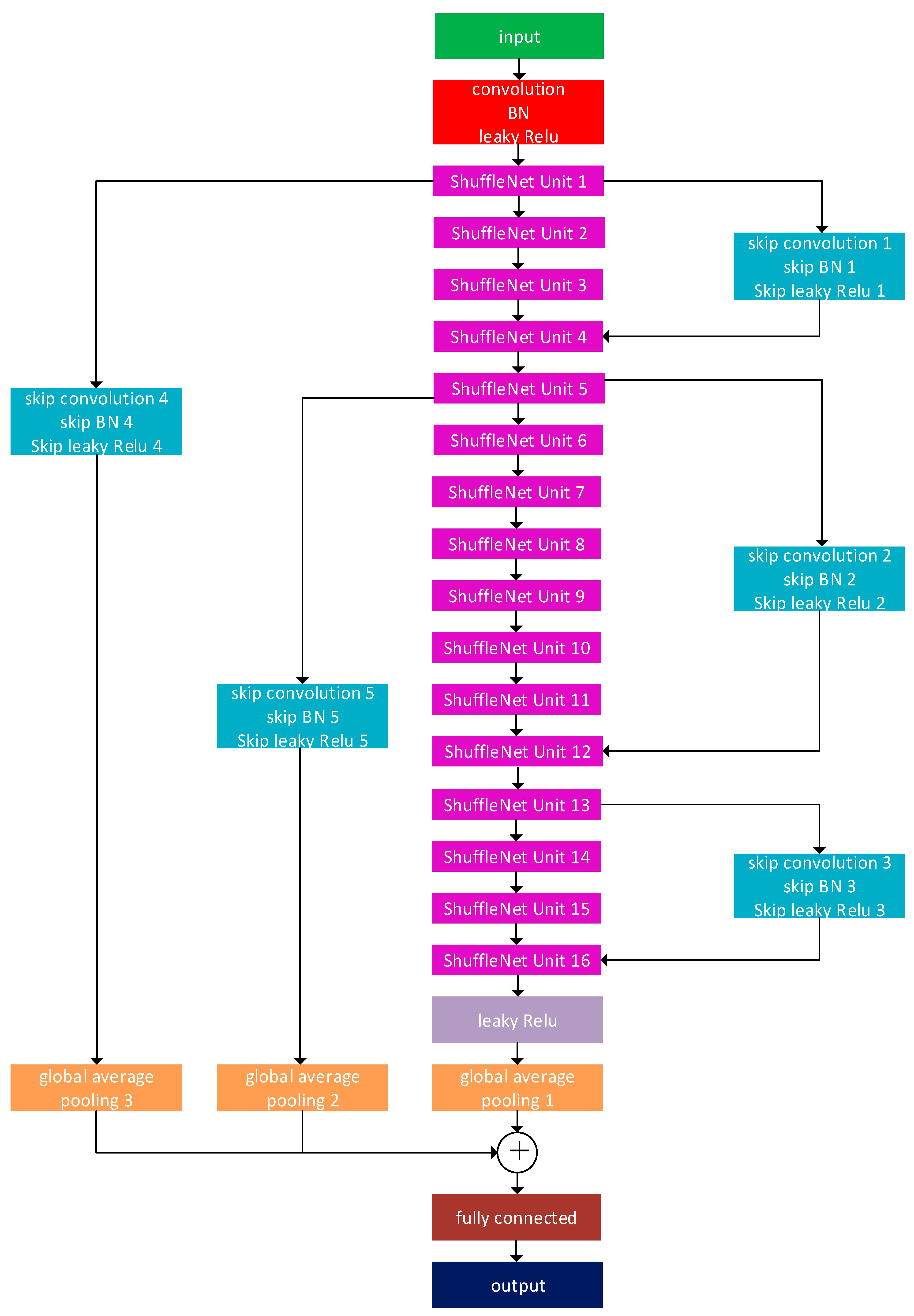
Figure 3 shows the final architecture of the proposed wide-ShuffleNet. ShuffleNet 1, 5, and 13 are stride units, whereas the others are the nonstride units. In three skip connections, we use three skip convolution layers at the same kernel size of 1 × 1 to connect the input layers of ShuffleNet units: 1, 5, 13, and an output layer of the ShuffleNet units: 4, 12, 16. Skip convolution layers: 1, 2, 3, 4, and 5 have 136, 272, 544, 544, and 544 filters, respectively. The stride for all skip convolution layers is equal to 2.

Additionally, we insert the batch normalization (BN) layer after every skip convolution layer due to some reasons. DL training process becomes quick when applying BN. Increasing the deep of the network means that the training process gets more challenging because of many problems faced while training. The architecture provides greater test data precision with the BN layer than the original model (without this layer). BN decreases the internal covariate shift; thus, improving the performance of the network. The classification accuracy significantly increases when applying BN. The position of the BN layer is after the convolutional layer and before the leaky ReLU layer. This structure speeds up the training and decreases testing and training time [73]. Furthermore, we replace all ReLU layers in all ShuffleNet units with the leaky ReLU layers. Leaky ReLU gives better results than the ReLU activation function (see reference [74]).

4. Experiment

In this section, we present the numerical results.

4.1. Datasets

The dataset plays an essential role in evaluating the performance of the proposed framework. We test the proposed method on the two datasets: HAM10000 and ISIC 2019.

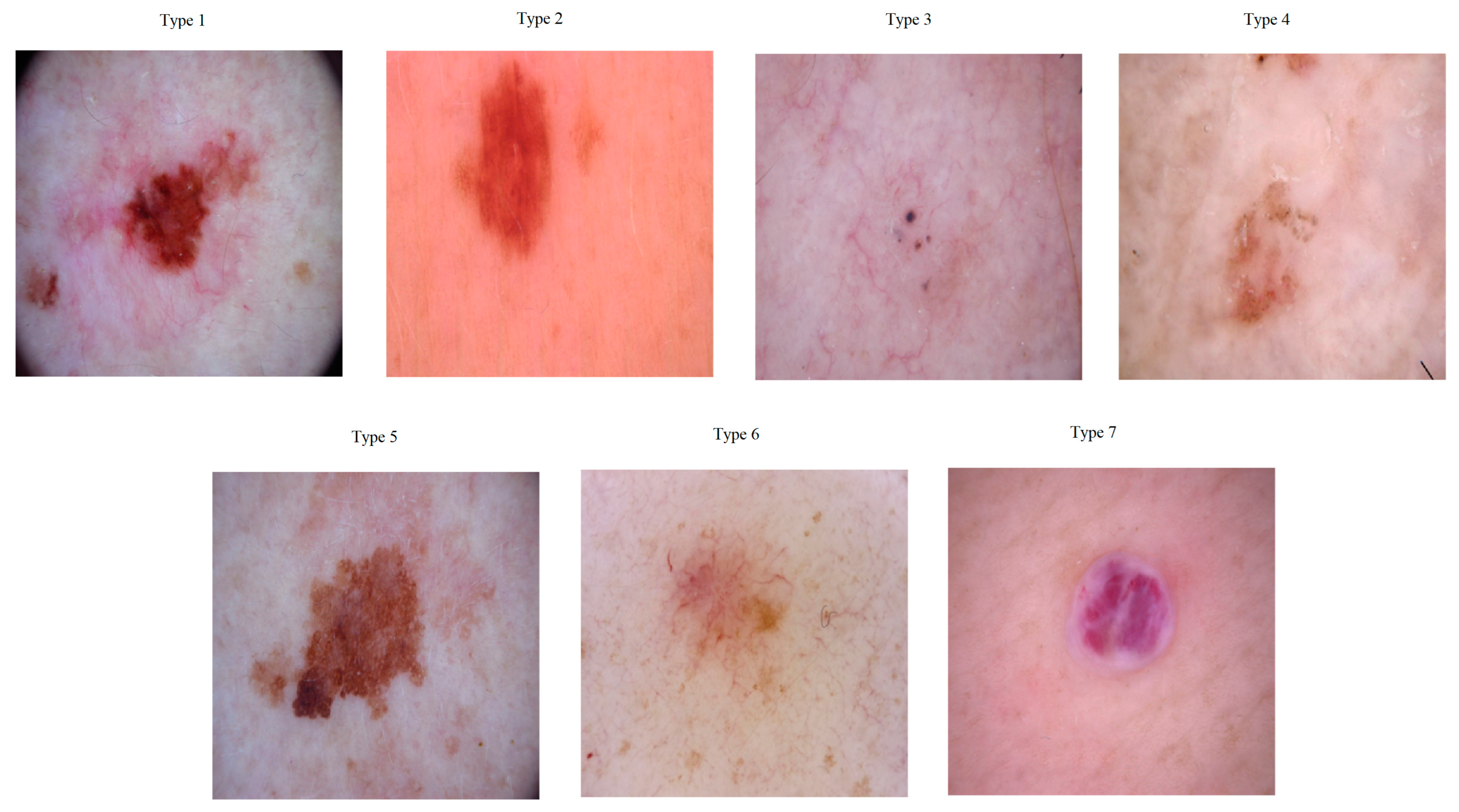
HAM10000 is the dermatoscopic database, which uses a benchmark dataset [75]. This database comprises more than 10,000 dermatoscopic pictures obtained from many people worldwide. The HAM10000 database also holds metadata formats like comma-separated-values data (.CSV), containing gender, age, and cell class. This dataset consists of seven different types of skin diseases: actinic keratoses and intraepithelial carcinoma (AKIEC), basal cell carcinoma (BCC), benign keratosis-like lesions (BKL), dermatofibroma (DF), melanoma (MEL), melanocytic Nevi (NV), and vascular lesions (VASC). The principal problem of the HAM10000 database is classes imbalance and the irregular distribution of skin disease numbers. NV class exceeds 70% of the total image numbers. This factor influences the training and creates an extreme imbalance database. The second large class is BKL, with approximately 13% of the pictures. The other classes contribute a minority number of the images. Especially, less than 2% of the total images belong to the DF class, which is the most difficult class for prediction. Figure 4 shows some sample images from the HAM10000 dataset. HAM10000 dataset is a part of the ISIC 2018 challenge with three tasks: lesion boundary segmentation (task 1), lesion attribute detection (task 2), disease classification (task 3).

The second dataset is the ISIC-2019 [76], consisting of 25,331 dermoscopic pictures belonging to eight categories: AKIEC, BCC, BKL, DF, MEL, NV, VASC, and squamous cell carcinoma (SCC). ISIC-2019 data are obtained from the following sources: BCN_20000 Dataset, HAM10000 Dataset, and MSK Dataset. The ISIC-2019 challenge has only one task: disease classification.

Table 2. Class distribution in the HAM10000 and ISIC 2019 datasets.

Class Name	HAM10000 Number of Images	ISIC2019 Number of Images
AKIEC	327	867
BCC	514	3323
BKL	1099	2624
DF	115	239
MEL	1113	4522
NV	6705	12,875
SCC	-	628
VASC	142	253
Total	10,015	25,331

gives the class distribution of the two datasets, HAM10000 and ISIC-2019.

4.2. Evaluation

We apply the following metrics to evaluate the performance of the proposed method.

$$Precision=\frac{TP}{TP+FP},$$

(12)

$$Sensitivity=\frac{TP}{TP+FN},$$

(13)

$$Specificity=\frac{TN}{TN+FP},$$

$$F1-score=2\times \frac{Precision\times Sensitivity}{Precision+Sensitivity},$$

(14)

$$Accuracy=\frac{TP+TN}{TP+FP+TN+FN},$$

(15)

where $TN$ is the true negative, $TP$ is the true positive, $FN$ is the false negative, and $FP$ is the false positive.

4.3. Implementation Details

The original HAM10000 and ISIC-2019 databases can be downloaded from the link in the Data Availability Statement. All tests were conducted on the i7 8700 PC, with 32 GB memory, GPU NVIDIA 1070, MATLAB (9.8 (R2020a), Natick, MA, USA). We apply the initial learning rate at 0.001, the mini-batch at 32, and the momentum at 0.9 for SGD for network training. After every 20 epochs, we divide the learning rate by half.

4.4. Comparison of the HAM10000 and ISIC 2019 Datasets

We evaluate the proposed method with two big datasets, HAM10000 and ISIC 2019. Then, we compare the performance of the proposed framework and that of state-of-the-art approaches for the skin lesion classification task, including non-segmentation and segmentation approaches. We split two datasets into training and testing parts with the same amount mentioned in references [23,29,76]. The HAM10000 dataset is used in the first and second experiments, with the percentages of the testing parts being 20% and 10%, respectively. The third experiment utilizes the ISCI2019 dataset, with 10% of the total images belonging to the testing part. We implemented three different experiments to make a fair comparison between the proposed EW-FCM framework and other methods. The reason is that each method uses a different dataset and a different proportion of the testing data from the whole dataset. For example, Thurnhofer-Hemsi et al. [23] use 20% of the dataset as the testing data, while Srinivasu et al. [29] use only 10% for the testing data on the same dataset HAM10000.

4.4.1. Comparison with Non-Segmentation Methods

Table 3. Comparison with different methods on the HAM10000 and ISIC2019 datasets.

Experiment	Method	ACC
Experiment 1 HAM10000 (80% training, 20% testing)	PNASNet [77]	76.00%
	ResNet-50 + gcForest [78]	80.04%
	VGG-16 + GoogLeNet Ensemble [79]	81.50%
	Densenet-121 with SVM [80]	82.70%
	DenseNet-169 [80]	81.35%
	Bayesian DenseNet-169 [81]	83.59%
	Shifted MobileNetV2 [23]	81.90%
	Shifted GoogLeNet [23]	80.50%
	Shifted 2-Nets [23]	83.20%
	The proposed method	84.80%
Experiment 2 HAM 10000 (90% training, 10% testing)	HARTS [82]	77.00%
	FTNN [83]	79.00%
	CNN [84]	80.00%
	VGG19 [85]	81.00%
	MobileNet V1 [68]	82.00%
	MobileNet V2 [86]	84.00%
	MobileNet V2-LSTM [29]	85.34%
	The proposed method	86.33%
Experiment 3 ISIC 2019 (90% training, 10% testing)	VGG19 [85]	80.17%
	ResNet-152 [64]	84.15%
	Efficient-B0 [87]	81.75%
	Efficient-B7 [87]	84.87%
	The proposed method	82.56%

presents the classification results of all approaches in three experiments.

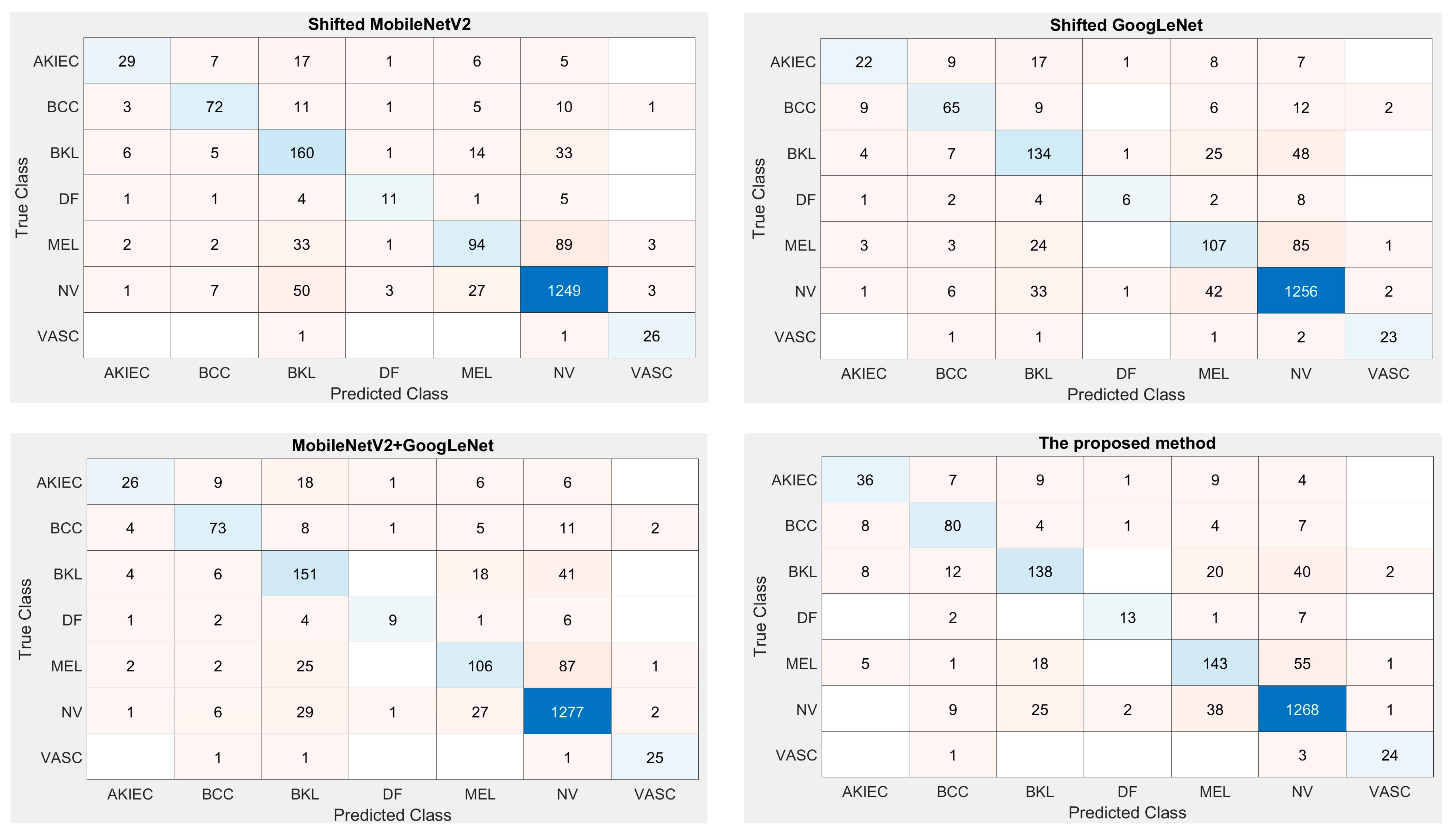
In the first experiment, the HAM10000 database is divided into two parts: one part with 8008 training images and the other part with 2007 testing images. Four methods in Table 3 provide the confusion matrix of the HAM10000 classification, including Shifted MobileNetV2, Shifted GoogLeNet, Shifted 2-Nets, and the proposed method. Shifted 2-Nets introduces an aggregate of enhanced CNN joined (ensemble of the DL approach) with a test-time regularly spaced shifting method for skin recognition. Shifted 2-Nets reached 83.20% accuracy (10.4 M parameters), whereas our framework produced 84.80% accuracy (1.8 M parameters). The proposed framework is more efficient than Shifted GoogLeNet, MobileNetV2, and Shifted 2-Nets. Figure 5 shows the confusion matrix of the four methods.

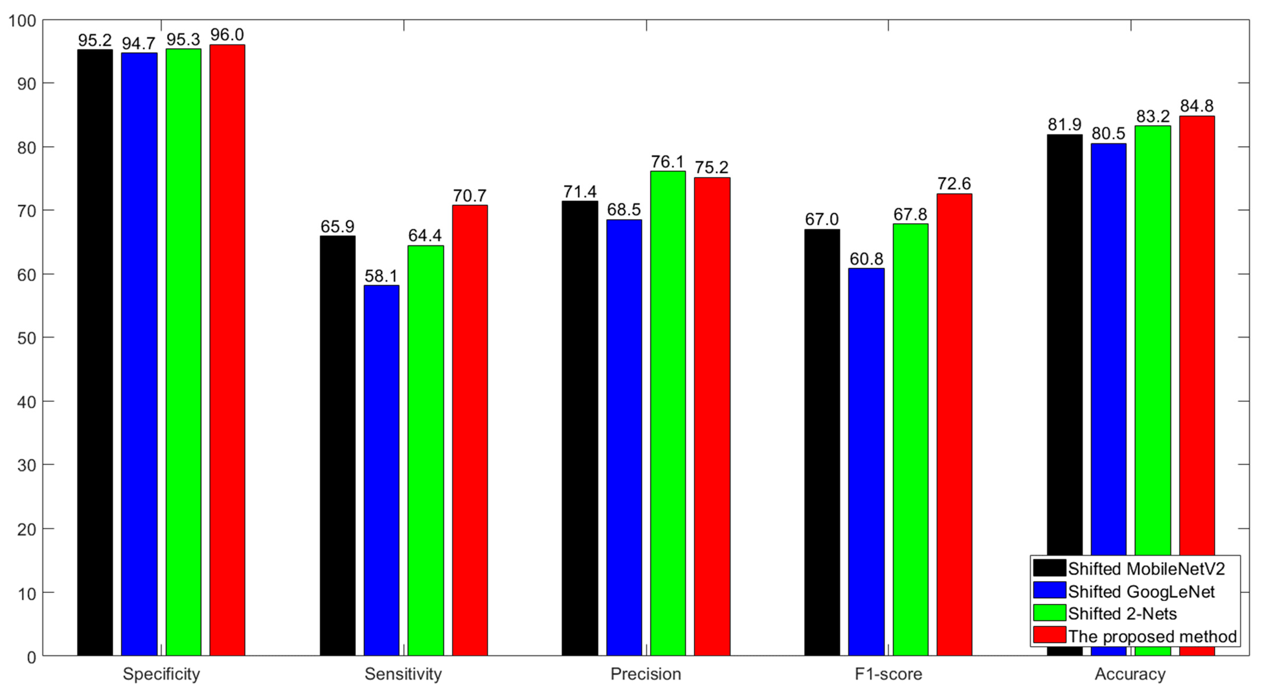
The first note is that the proposed method has a lower wrong classification than other methods. Additionally, the number of right predictions has improved for most categories: AKIEC, BCC, DF, and MEL categories. BKL, NV, and VASC are three experiments that our framework ranks as the third, second, and third positions among four approaches, respectively. We calculate the following metrics from the obtained confusion matrix: specificity, sensitivity, precision, and F1 score.

Table 4. Comparison with different methods on the HAM10000 dataset in the first experiment (macro-average).

	Methods
	Shifted MobileNetV2	Shifted GoogLeNet	Shifted 2-Nets	The Proposed Method
Specificity	95.20%	94.70%	95.30%	96.03%
Sensitivity	65.90%	58.10%	64.40%	70.71%
Precision	71.40%	68.50%	76.10%	75.15%
F1 score	67.00%	60.80%	67.80%	72.61%
Accuracy	81.90%	80.50%	83.20%	84.80%
Parameters	3.4 M	7 M	10.4 M	1.8 M

, which is visualized in Figure 6, presents our proposed framework’s performance and various approaches with five metrics: accuracy, specificity, sensitivity, precision, and F1 score (macro-average).

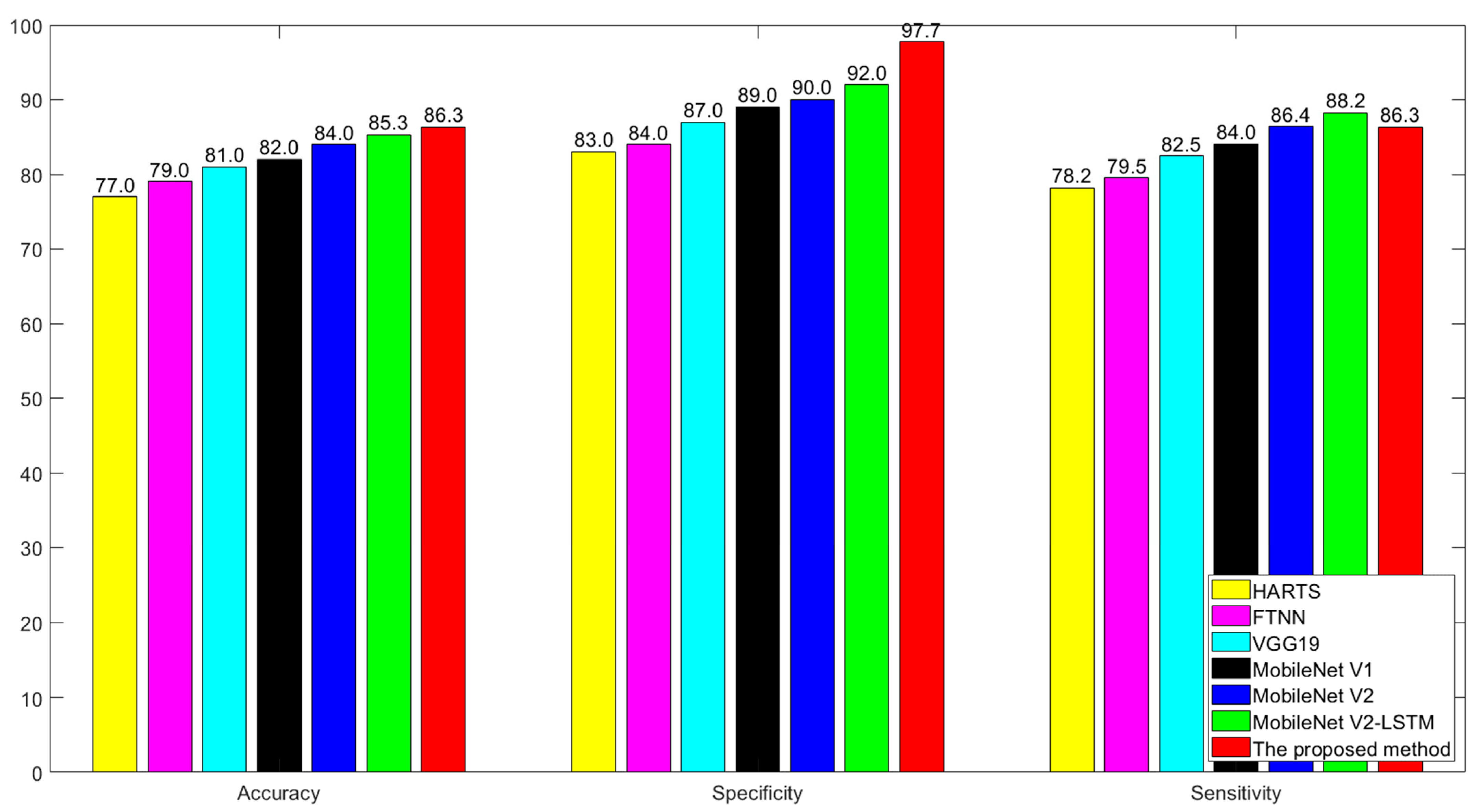
In the second experiment, the HAM10000 database is split into two parts: 90% of the total images are the training part, and the rest are the testing part. None of the methods in Table 3 in the second experiment yield the precision, F1 score, and confusion matrix (micro-average metric). We use three metrics to evaluate the performance of various methods: accuracy, sensitivity, and specificity.

Table 5. Comparison with different methods on the HAM10000 dataset in the second experiment (micro-average).

Method	Accuracy	Specificity	Sensitivity	Parameters
HARTS [82]	77.00%	83.00%	78.21%	-
FTNN [83]	79.00%	84.00%	79.54%	-
VGG19 [85]	81.00%	87.00%	82.46%	143 M
MobileNet V1 [68]	82.00%	89.00%	84.04%	4.2 M
MobileNet V2 [86]	84.00%	90.00%	86.41%	3.4 M
MobileNet V2-LSTM [29]	85.34%	92.00%	88.24%	$\approx$3.4 M
The proposed method	86.33%	97.72%	86.33%	1.8 M

presents the outcomes of all approaches. Figure 7 visualizes the results of Table 5. Our framework achieves the highest performance in terms of accuracy and specificity. Meanwhile, the MobileNet V2 with long short-term memory (LSTM) [29] component has the highest sensitivity. MobileNet V2 improves efficiency more than the first version MobileNet V1. Consequently, the number of parameters decreases 19% from 4.2 to 3.4 M. MobileNet V2 is approximately two times the parameters of our framework (1.8 M), even with lower parameters. Additionally, VGG19 has the highest number of parameters with about 143 M (79 times the proposed method). This comparison confirms the efficiency of the proposed framework.

In the third experiment, we follow the dataset divided according to the previous study [76]. The authors in reference [76] tested the skin classification on the ISIC-2019 dataset with different transfer learning models, such as state-of-the-art architecture EfficientNet. EfficientNet has eight models that start from B0 to B7 and achieve better efficiency and accuracy than earlier ConvNets. EfficientNet employs swish activation instead of applying the ReLU function (see reference [76]).

Table 6. Comparison with different methods on the ISIC2019 dataset in the third experiment (micro-average).

Method	Accuracy	Specificity	Sensitivity	Parameters
VGG19 [85]	80.17%	-	-	143 M
ResNet-152 [64]	84.15%	-	-	50 M
Efficient-B0 [87]	81.75%	-	-	5 M
Efficient-B7 [87]	84.87%			66 M
The proposed method	82.56%	97.51%	82.56%	1.8 M

compares all approaches. All methods provide only the accuracy metric, except the proposed methods. EfficientNetB0 uses a small number of parameters. It is the simplest of all eight architectures in EfficientNet. However, the total parameters of EfficientNet-B0 are approximately three times that of our method (5 M compared with 1.8 M), whereas the accuracy is lower (81.75% compared with 82.56%). EfficientNet-B7 and ResNet-152 are the first and second rank in terms of accuracy, respectively. Both architectures have high parameters (66 and 50 M, respectively) and achieved a better result than our method (the proposed network uses less than 4% of the parameters compared to these two models). VGG19 is the worst method with the highest parameters (143 M) and the lowest accuracy (80.17%).

We have already compared different methods in three experiments. Even with the highest efficiency result, our method has a weakness that could not control the imbalanced classes of two datasets: HAM10000 and ISIC2019. Data sampling methods, which are the future research work, can balance the classes distribution.

4.4.2. Comparison with Segmentation Methods

The proposed method has higher accuracy and is more efficient than other non-segmentation approaches. In this section, we compare the proposed EW-FCM with other segmentation techniques, such as non-DL and DL segmentation methods. All segmentation methods use the full lesion image (background and foreground) as the input image for the classification network.

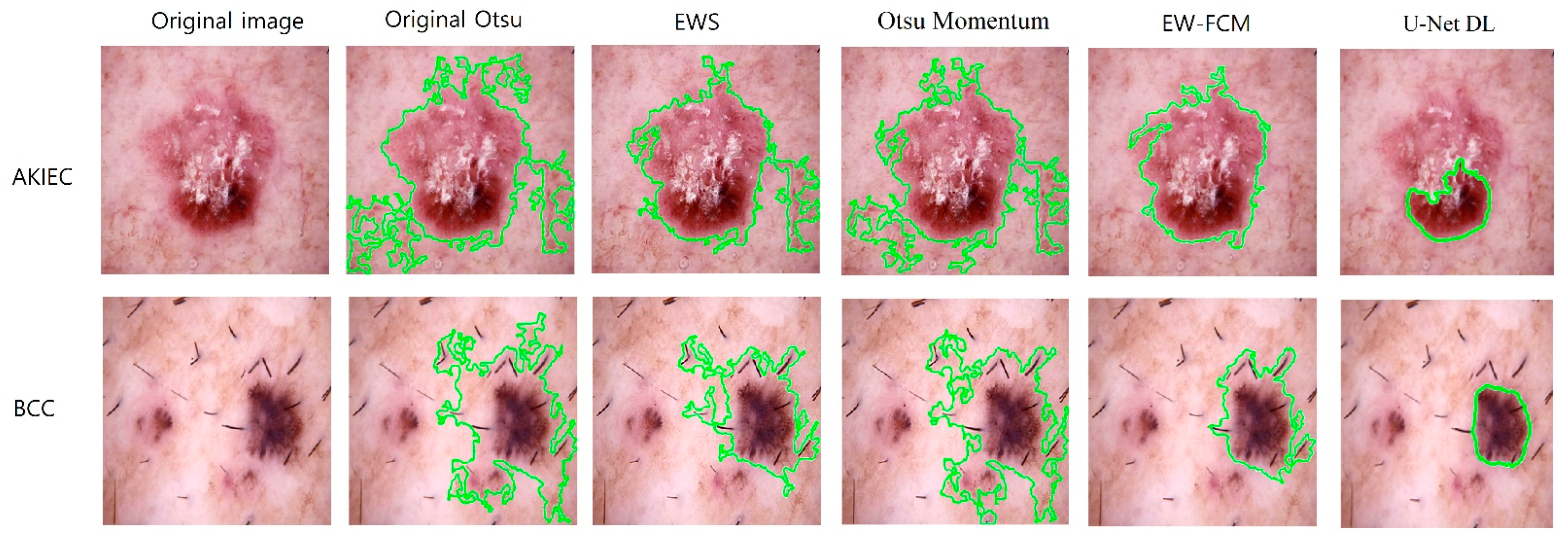
First, we compare the proposed EW-FCM with other non-DL methods, such as the original Otsu, Otsu momentum, an EW scheme.

Table 7. Comparison with segmentation methods on the HAM10000 and ISIC2019 datasets (micro-average).

Experiment	Method	ACC	Sensitivity	Specificity
Experiment 1 HAM10000 (80% training, 20% testing)	Original Otsu + wide-ShuffleNet	79.62%	79.62%	96.60%
	Otsu Momentum [57] + wide-ShuffleNet	81.51%	81.51%	96.92%
	Image Entropy [56] + wide-ShuffleNet	83.91%	83.91%	97.32%
	U-Net + wide-ShuffleNet	85.10%	85.10%	97.52%
	U-Net + EfficientNet-B0 [54]	85.65%	85.65%	97.61%
	FrCN + Inception-ResNet-v2 [55]	87.74%	-	-
	FrCN + Inception-v3 [55]	88.05%	-	-
	FrCN + DenseNet-201 [55]	88.70%	-	-
	EW-FCM + wide-ShuffleNet	84.80%	84.80%	97.48%
Experiment 2 HAM 10000 (90% training, 10% testing)	Original Otsu + wide-ShuffleNet	80.14%	80.14%	96.69%
	Otsu Momentum [57] + wide-ShuffleNet	82.54%	82.54%	97.09%
	Image Entropy [56] + wide-ShuffleNet	84.83%	84.83%	97.47%
	EW-FCM + wide-ShuffleNet	86.33%	86.33%	97.72%
Experiment 3 ISIC 2019 (90% training, 10% testing)	Original Otsu + wide-ShuffleNet	78.55%	78.55%	96.94%
	Otsu Momentum [57] + wide-ShuffleNet	80.34%	80.34%	97.19%
	Image Entropy [56] + wide-ShuffleNet	81.20%	81.20%	97.31%
	EW-FCM + wide-ShuffleNet	82.56%	82.56%	97.51%

presents the results. EW-FCM achieved the highest accuracy among non-DL segmentation approaches. Figure 8 shows the segmentation results of various segmentation methods.

Second, we compare the proposed EW-FCM with DL segmentation methods. Al-Masni et al. [55] provides only the accuracy of the training of the ISIC 2018 task 3 (HAM10000 dataset). Moreover, Al-Masni et al. [55] uses DL FrCN to segment the skin lesion and classify full lesion images with various networks, such as Inception-ResNet-v2, DenseNet-201, and Inception-v3. Meanwhile, Son et al. [54] crop the segmented image with U-Net and input the result to Efficient-B0 for classification. We adopt the idea of U-Net and Efficient-B0 in [54] to evaluate the HAM10000 dataset using the U-Net as a segmentation method with full lesion image (background and foreground). EW-FCM achieved a lower accuracy than the DL segmentation methods (see Table 7); it also achieved higher results than non-DL segmentation methods. There are two main drawbacks of the DL segmentation methods. First, creating a labeled training database is the primary challenge to creating a DL segmentation network in which each picture has an associated ground truth. A massive effort of dermatologists is used to obtain this ground truth pixel-wise segmentation. Meanwhile, the proposed EW-FCM uses a threshold technique for image segmentation and does not depend on the ground truth. As a result, we cannot calculate the quantitative analysis with the EW-FCM segmentation technique (such as using the Jaccard index). Second, the complexity increases when using DL for segmentation and classification. For instance, the total parameters of the DL segmentation U-Net and DL classification Efficient-B0 are 12.7 M (7.7 M + 5 M = 12.7 M). EW-FCM uses DL only for the classification state, thus decreasing the complexity and being suitable with a portable system.

Next, we evaluate the performance of the skin classification with various classifiers and present the results in

Table 8. Comparison with different networks on the HAM10000 and ISIC2019 datasets (micro-average).

Experiment	Method	ACC	Sensitivity	Specificity
Experiment 1 HAM10000 (80% training, 20% testing)	Original Image + ShuffleNet	76.83%	76.83%	96.14%
	Original Image + wide-ShuffleNet	77.88%	77.88%	96.31%
	EW-FCM + ShuffleNet	83.66%	83.66%	97.28%
	EW-FCM + wide-ShuffleNet	84.80%	84.80%	97.48%
	EW-FCM + EfficientNet-B0	85.50%	85.50%	97.58%
Experiment 2 HAM 10000 (90% training, 10% testing)	Original Image + ShuffleNet	77.25%	77.25%	96.21%
	Original Image + wide-ShuffleNet	78.64%	78.64%	96.44%
	EW-FCM + ShuffleNet	84.43%	84.43%	97.41%
	EW-FCM + wide-ShuffleNet	86.33%	86.33%	97.72%
	EW-FCM + EfficientNet-B0	87.23%	87.23%	97.87%
Experiment 3 ISIC 2019 (90% training, 10% testing)	Original Image + ShuffleNet	74.23%	74.23%	96.32%
	Original Image + wide-ShuffleNet	75.73%	75.73%	96.53%
	EW-FCM + ShuffleNet	81.62%	81.62%	97.38%
	EW-FCM + wide-ShuffleNet	82.56%	82.56%	97.51%
	EW-FCM + EfficientNet-B0	84.66%	84.66%	97.81%

. The proposed method improves the skin classification for two reasons: wide-ShuffleNet is better than ShuffleNet, and the new segmentation technique is better than the original image. Efficient-B0 has the highest accuracy, but its parameters increase approximately three times compared to wide-ShuffleNet. In future studies, we will investigate the performance of EW-FCM with ShuffleNet V2 (2.4 M parameters) and compare it with the proposed wide-ShuffleNet (1.8 M parameters).

5. Conclusions

Skin cancer is one of the most dangerous diseases in humans. The automated classification of skin lesions using DL will save time for physicians and increase the curing rate. Typical DL frameworks require high parameters and cannot work on the mobile system. Hence, developing the lightweight DL framework for skin lesion classification is essential.

In this paper, we propose a novel method for skin lesion classification. Our lightweight method improves the limitation of evaluating a small number of skin lesion images in the past. The numerical results show that the proposed framework is more efficient and accurate than the 20 other approaches (see Table 3). The proposed method reduces the number of the parameters to approximately 79 times that of another method (VGG19) while maintaining higher accuracy. Additionally, the proposed method achieves higher accuracy than other non-segmentation and non-DL segmentation methods and the approximate results at the level of the DL segmentation methods while reducing the complexity of the DL segmentation methods. Our framework does not require ground truth for image segmentation, whereas DL segmentation methods cannot work without ground truth. Thus, the proposed method decreases the effort of the dermatologists to manually outline the ground truth pixel-wise segmentation. We create an accurate and efficient framework by combining the new EW-FCM segmentation technique and wide-ShuffleNet.

We will compare the proposed framework with more networks in future work. Another future direction for research and development is to integrate the proposed method into real-world problems like the mobile healthcare system.

References

- Rey-Barroso, L.; Peña-Gutiérrez, S.; Yáñez, C.; Burgos-Fernández, F.J.; Vilaseca, M.; Royo, S. Optical technologies for the improvement of skin cancer diagnosis: A review. Sensors 2021, 21, 252. [Google Scholar] [CrossRef]
- Hosny, K.M.; Kassem, M.A.; Foaud, M.M. Classification of skin lesions using transfer learning and augmentation with Alex-net. PLoS ONE 2019, 14, e0217293. [Google Scholar] [CrossRef] [PubMed] [Green Version]
- Zicari, R.V.; Ahmed, S.; Amann, J.; Braun, S.A.; Brodersen, J.; Bruneault, F.; Wurth, R. Co-Design of a trustworthy AI System in healthcare: Deep learning based skin lesion classifier. Front. Hum. Dyn. 2021, 3, 40. [Google Scholar] [CrossRef]
- Mishra, N.; Celebi, M. An overview of melanoma detection in dermoscopy images using image processing and machine learning. arXiv 2016, arXiv:1601.07843. [Google Scholar]
- World Health Organization. Radiation: Ultraviolet (UV) Radiation and Skin Cancer. Available online: https://www.who.int/news-room/questions-and-answers/item/radiation-ultraviolet-(uv)-radiation-and-skin-cancer#:~:text=Currently%2C%20between%202%20and%203,skin%20cancer%20in%20their%20lifetime (accessed on 19 October 2021).
- Jerant, A.F.; Johnson, J.T.; Sheridan, C.D.; Caffrey, T.J. Early detection and treatment of skin cancer. Am. Fam. Physician 2000, 62, 357–368. [Google Scholar]
- Trufant, J.; Jones, E. Skin cancer for primary care. In Common Dermatologic Conditions in Primary Care; John, J.R., Edward, F.R., Jr., Eds.; Springer: Cham, Switzerland, 2019; pp. 171–208. [Google Scholar]
- Barata, C.; Celebi, M.E.; Marques, J.S. A survey of feature extraction in dermoscopy image analysis of skin cancer. IEEE J. Biomed. Health Inform. 2019, 23, 1096–1109. [Google Scholar] [CrossRef] [PubMed]
- Celebi, M.E.; Kingravi, H.A.; Uddin, B.; Iyatomi, H.; Aslandogan, Y.A.; Stoecker, W.V.; Moss, R.H. A methodological approach to the classification of dermoscopy images. Comput. Med. Imaging Graph. 2007, 31, 362–373. [Google Scholar] [CrossRef] [Green Version]
- Tommasi, T.; La Torre, E.; Caputo, B. Melanoma recognition using representative and discriminative kernel classifiers. In Proceedings of the International Workshop on Computer Vision Approaches to Medical Image Analysis (CVAMIA), Graz, Austria, 12 May 2006; pp. 1–12. [Google Scholar] [CrossRef]
- Pathan, S.; Prabhu, K.G.; Siddalingaswamy, P.C. A methodological approach to classify typical and atypical pigment network patterns for melanoma diagnosis. Biomed. Signal Process. Control 2018, 44, 25–37. [Google Scholar] [CrossRef]
- Taner, A.; Öztekin, Y.B.; Duran, H. Performance analysis of deep learning CNN models for variety classification in hazelnut. Sustainability 2021, 13, 6527. [Google Scholar] [CrossRef]
- Wang, W.; Siau, K. Artificial intelligence, machine learning, automation, robotics, future of work and future of humanity: A review and research agenda. J. Database Manag. 2019, 30, 61–79. [Google Scholar] [CrossRef]
- Samuel, A.L. Some studies in machine learning using the game of checkers. II—Recent progress. In Computer Games I; Springer: Berlin/Heidelberg, Germany, 1988; pp. 366–400. [Google Scholar]
- Liu, W.; Wang, Z.; Liu, X.; Zeng, N.; Liu, Y.; Alsaadi, F.E. A survey of deep neural network architectures and their applications. Neurocomputing 2017, 234, 11–26. [Google Scholar] [CrossRef]
- Qiu, Z.; Chen, J.; Zhao, Y.; Zhu, S.; He, Y.; Zhang, C. Variety identification of single rice seed using hyperspectral imaging combined with convolutional neural network. Appl. Sci. 2018, 8, 212. [Google Scholar] [CrossRef] [Green Version]
- Acquarelli, J.; Van, L.T.; Gerretzen, J.; Tran, T.N.; Buydens, L.M.; Marchiori, E. Convolutional neural networks for vibrational spectroscopic data analysis. Anal. Chim. Acta 2017, 954, 22–31. [Google Scholar] [CrossRef] [PubMed] [Green Version]
- Zhang, X.; Lin, T.; Xu, J.; Luo, X.; Ying, Y. DeepSpectra: An end-to-end deep learning approach for quantitative spectral analysis. Anal. Chim. Acta 2019, 1058, 48–57. [Google Scholar] [CrossRef] [PubMed]
- Yang, X.; Ye, Y.; Li, X.; Lau, R.Y.; Zhang, X.; Huang, X. Hyperspectral image classification with deep learning models. IEEE Trans. Geosci. Remote Sens. 2018, 56, 5408–5423. [Google Scholar] [CrossRef]
- Yu, X.; Tang, L.; Wu, X.; Lu, H. Nondestructive freshness discriminating of shrimp using visible/near-infrared hyperspectral imaging technique and deep learning algorithm. Food Anal. Methods 2018, 11, 768–780. [Google Scholar] [CrossRef]
- Yue, J.; Mao, S.; Li, M. A deep learning framework for hyperspectral image classification using spatial pyramid pooling. Remote Sens. Lett. 2016, 7, 875–884. [Google Scholar] [CrossRef]
- Signoroni, A.; Savardi, M.; Baronio, A.; Benini, S. Deep learning meets hyperspectral image analysis: A multidisciplinary review. J. Imaging 2019, 5, 52. [Google Scholar] [CrossRef] [Green Version]
- Thurnhofer-Hemsi, K.; López-Rubio, E.; Domínguez, E.; Elizondo, D.A. Skin lesion classification by ensembles of deep convolutional networks and regularly spaced shifting. IEEE Access 2021, 9, 112193–112205. [Google Scholar] [CrossRef]
- Litjens, G.; Kooi, T.; Bejnordi, B.E.; Setio, A.A.A.; Ciompi, F.; Ghafoorian, M.; van der Laak, J.A.; van Ginneken, B.; Sánchez, C.I. A survey on deep learning in medical image analysis. Med. Image Anal. 2017, 42, 60–88. [Google Scholar] [CrossRef] [PubMed] [Green Version]
- Cui, C.; Thurnhofer-Hemsi, K.; Soroushmehr, R.; Mishra, A.; Gryak, J.; Dominguez, E.; Najarian, K.; Lopez-Rubio, E. Diabetic wound segmentation using convolutional neural networks. In Proceedings of the 41th Annual International Conference of the IEEE Engineering in Medicine and Biology Society (EMBC), Berlin, Germany, 23–27 July 2019; pp. 1002–1005. [Google Scholar]
- Thurnhofer-Hemsi, K.; Domínguez, E. Analyzing digital image by deep learning for melanoma diagnosis. In Advances in Computational Intelligence; Rojas, I., Joya, G., Catala, A., Eds.; Springer: Cham, Switzerland, 2019; pp. 270–279. [Google Scholar]
- Thurnhofer-Hemsi, K.; Domínguez, E. A convolutional neural network framework for accurate skin cancer detection. Neural Process. Lett. 2021, 53, 3073–3093. [Google Scholar] [CrossRef]
- Codella, N.C.; Gutman, D.; Celebi, M.E.; Helba, B.; Marchetti, M.A.; Dusza, S.W.; Halpern, A. Skin lesion analysis toward melanoma detection: A challenge at the 2017 international symposium on biomedical imaging (ISBI), hosted by the international skin imaging collaboration (ISIC). In Proceedings of the 2018 IEEE 15th International Symposium on Biomedical Imaging (ISBI 2018), Washington, DC, USA, 4–7 April 2018; pp. 168–172. [Google Scholar] [CrossRef] [Green Version]
- Srinivasu, P.N.; SivaSai, J.G.; Ijaz, M.F.; Bhoi, A.K.; Kim, W.; Kang, J.J. Classification of skin disease using deep learning neural networks with MobileNet V2 and LSTM. Sensors 2021, 21, 2852. [Google Scholar] [CrossRef] [PubMed]
- Dang, Y.; Jiang, N.; Hu, H.; Ji, Z.; Zhang, W. Image classification based on quantum K-nearest-neighbor algorithm. Quantum Inf. Process. 2018, 17, 239. [Google Scholar] [CrossRef]
- Sumithra, R.; Suhil, M.; Guru, D.S. Segmentation and classification of skin lesions for disease diagnosis. Procedia Comput. Sci. 2015, 45, 76–85. [Google Scholar] [CrossRef] [Green Version]
- Sajid, P.M.; Rajesh, D.A. Performance evaluation of classifiers for automatic early detection of skin cancer. J. Adv. Res. Dyn. Control. Syst. 2018, 10, 454–461. [Google Scholar]
- Zhang, S.; Wu, Y.; Chang, J. Survey of image recognition algorithms. In Proceedings of the 2020 IEEE 4th Information Technology, Networking, Electronic and Automation Control Conference (ITNEC), Chongqing, China, 12–14 June 2020; pp. 542–548. [Google Scholar] [CrossRef]
- Alam, M.; Munia, T.T.K.; Tavakolian, K.; Vasefi, F.; MacKinnon, N.; Fazel-Rezai, R. Automatic detection and severity measurement of eczema using image processing. In Proceedings of the 2016 38th Annual International Conference of the IEEE Engineering in Medicine and Biology Society (EMBC), Orlando, FL, USA, 16–20 August 2016; pp. 1365–1368. [Google Scholar] [CrossRef]
- Immagulate, I.; Vijaya, M.S. Categorization of non-melanoma skin lesion diseases using support vector machine and its variants. Int. J. Med. Imaging 2015, 3, 34–40. [Google Scholar] [CrossRef] [Green Version]
- Upadhyay, P.K.; Chandra, S. An improved bag of dense features for skin lesion recognition. J. King Saud Univ. Comput. Inf. Sci. 2019; in press. [Google Scholar] [CrossRef]
- Awad, M.; Khanna, R. Support vector machines for classification. In Efficient Learning Machines; Apress: Berkeley, CA, USA, 2015; pp. 39–66. [Google Scholar]
- Hsu, W. Bayesian classification. In Encyclopedia of Database Systems, 2nd ed.; Liu, L., Özsu, M.T., Eds.; Springer: New York, NY, USA, 2018; pp. 3854–3857. [Google Scholar]
- Tahmassebi, A.; Gandomi, A.; Schulte, M.; Goudriaan, A.; Foo, S.; Meyer-Base, A. Optimized naive-bayes and decision tree approaches for fMRI smoking cessation classification. Complexity 2018, 2018, 2740817. [Google Scholar] [CrossRef]
- Seixas, J.L.; Mantovani, R.G. Decision trees for the detection of skin lesion patterns in lower limbs ulcers. In Proceedings of the 2016 International Conference on Computational Science and Computational Intelligence (CSCI), Las Vegas, NV, USA, 15–17 December 2018; pp. 677–681. [Google Scholar] [CrossRef]
- Arasi, M.A.; El-Horbaty, E.S.M.; El-Sayed, A. Classification of dermoscopy images using naive bayesian and decision tree techniques. In Proceedings of the 2018 1st Annual International Conference on Information and Sciences (AiCIS), Fallujah, Iraq, 20–21 November 2018; pp. 7–12. [Google Scholar] [CrossRef]
- Hamad, M.A.; Zeki, A.M. Accuracy vs. cost in decision trees: A survey. In Proceedings of the 2018 International Conference on Innovation and Intelligence for Informatics, Computing, and Technologies (3ICT), Sakhier, Bahrain, 18–20 November 2018; pp. 1–4. [Google Scholar] [CrossRef]
- Serte, S.; Demirel, H. Gabor wavelet-based deep learning for skin lesion classification. Comput. Biol. Med. 2019, 113, 103423. [Google Scholar] [CrossRef]
- Menegola, A.; Tavares, J.; Fornaciali, M.; Li, L.T.; Avila, S.; Valle, E. RECOD Titans at ISIC Challenge 2017. 2017. Available online: https://arxiv.org/abs/1703.04819 (accessed on 19 October 2021).
- Han, S.S.; Kim, M.S.; Lim, W.; Park, G.H.; Park, I.; Chang, S.E. Classification of the clinical images for benign and malignant cutaneous tumors using a deep learning algorithm. J. Investig. Dermatol. 2018, 138, 1529–1538. [Google Scholar] [CrossRef] [Green Version]
- Esteva, A.; Kuprel, B.; Novoa, R.A.; Ko, J.; Swetter, S.M.; Blau, H.M.; Thrun, S. Dermatologist-level classification of skin cancer with deep neural networks. Nature 2017, 542, 115–118. [Google Scholar] [CrossRef] [PubMed]
- Fujisawa, Y.; Otomo, Y.; Ogata, Y.; Nakamura, Y.; Fujita, R.; Ishitsuka, Y.; Fujimoto, M. Deep-learning-based, computer-aided classifier developed with a small dataset of clinical images surpasses boardcertified dermatologists in skin tumour diagnosis. Br. J. Dermatol. 2019, 180, 373–381. [Google Scholar] [CrossRef]
- Mahbod, A.; Ecker, R.; Ellinger, I. Skin lesion classification using hybrid deep neural networks. In Proceedings of the ICASSP 2019–2019 IEEE International Conference on Acoustics, Speech and Signal Processing (ICASSP), Brighton, UK, 12–17 May 2019; pp. 1229–1233. [Google Scholar]
- Harangi, B. Skin lesion classification with ensembles of deep convolutional neural networks. Biomed. Inf. 2018, 86, 25–32. [Google Scholar] [CrossRef] [PubMed]
- Nyíri, T.; Kiss, A. Novel ensembling methods for dermatological image classification. In Proceedings of the International Conference on Theory and Practice of Natural Computing, Dublin, Ireland, 12–14 December 2018; pp. 438–448. [Google Scholar]
- Matsunaga, K.; Hamada, A.; Minagawa, A.; Koga, H. Image classification of melanoma, nevus and seborrheic keratosis by deep neural network ensemble. arXiv 2017, arXiv:1703.03108. [Google Scholar]
- Li, Y.; Shen, L. Skin lesion analysis towards melanoma detection using deep learning network. Sensors 2018, 18, 556. [Google Scholar] [CrossRef] [Green Version]
- Díaz, I.G. Incorporating the knowledge of dermatologists to convolutional neural networks for the diagnosis of skin lesions. arXiv 2017, arXiv:1703.01976v1. [Google Scholar]
- Son, H.M.; Jeon, W.; Kim, J.; Heo, C.Y.; Yoon, H.J.; Park, J.U.; Chung, T.M. AI-based localization and classification of skin disease with erythema. Sci. Rep. 2021, 11, 1–14. [Google Scholar] [CrossRef]
- Al-Masni, M.A.; Kim, D.H.; Kim, T.S. Multiple skin lesions diagnostics via integrated deep convolutional networks for segmentation and classification. Comput. Methods Programs Biomed. 2020, 190, 105351. [Google Scholar] [CrossRef]
- Truong, M.T.N.; Kim, S. Automatic image thresholding using Otsu’s method and entropy weighting scheme for surface defect detection. Soft Comput. 2018, 22, 4197–4203. [Google Scholar] [CrossRef]
- Zhan, Y.; Zhang, G. An improved OTSU algorithm using histogram accumulation moment for ore segmentation. Symmetry 2019, 11, 431. [Google Scholar] [CrossRef] [Green Version]
- Zade, S. Medical-Image-Segmentation. Available online: https://github.com/mathworks/Medical-Image-Segmentation/releases/tag/v1.0 (accessed on 19 October 2021).
- Krizhevsky, A.; Sutskever, I.; Hinton, G.E. Imagenet classification with deep convolutional neural networks. In Proceedings of the 25th International Conference on Neural Information Processing Systems, Lake Tahoe, NV, USA, 3–6 December 2012; pp. 1097–1105. [Google Scholar]
- Ren, S.; He, K.; Girshick, R.; Sun, J. Faster R-CNN: Towards real-time object detection with region proposal networks. In Proceedings of the Advances in Neural Information Processing Systems 28 (NIPS 2015), Montreal, QC, Canada, 7–12 December 2015; pp. 91–99. [Google Scholar]
- Zhang, X.; Zhou, X.; Lin, M.; Sun, J. Shufflenet: An extremely efficient convolutional neural network for mobile devices. arXiv 2017, arXiv:1707.01083. [Google Scholar]
- He, K.; Sun, J. Convolutional neural networks at constrained time cost. In Proceedings of the IEEE Conference on Computer Vision and Pattern Recognition, Boston, MA, USA, 7–12 June 2015; pp. 5353–5360. [Google Scholar] [CrossRef] [Green Version]
- Szegedy, C.; Liu, W.; Jia, Y.; Sermanet, P.; Reed, S.; Anguelov, D.; Erhan, D.; Vanhoucke, V.; Rabinovich, A. Going deeper with convolutions. In Proceedings of the IEEE Conference on Computer Vision and Pattern Recognition, Boston, MA, USA, 8–10 June 2015; pp. 1–9. [Google Scholar] [CrossRef] [Green Version]
- He, K.; Zhang, X.; Ren, S.; Sun, J. Deep residual learning for image recognition. In Proceedings of the IEEE Conference on Computer Vision and Pattern Recognition, Las Vegas, NV, USA, 27–30 June 2016; pp. 770–778. [Google Scholar] [CrossRef] [Green Version]
- He, K.; Zhang, X.; Ren, S.; Sun, J. Identity mappings in deep residual networks. In Proceedings of the European Conference on Computer Vision, Amsterdam, The Netherlands, 11–14 October 2016. [Google Scholar] [CrossRef] [Green Version]
- Iandola, F.N.; Han, S.; Moskewicz, M.W.; Ashraf, K.; Dally, W.J.; Keutzer, K. Squeezenet: Alexnet-level accuracy with 50× fewer parameters and 0.5 mb model size. arXiv 2016, arXiv:1602.07360. [Google Scholar]
- Xie, S.; Girshick, R.; Dollár, P.; Tu, Z.; He, K. Aggregated residual transformations for deep neural networks. arXiv 2016, arXiv:1611.05431. [Google Scholar]
- Howard, A.G.; Zhu, M.; Chen, B.; Kalenichenko, D.; Wang, W.; Weyand, T.; Adam, H. Mobilenets: Efficient convolutional neural networks for mobile vision applications. arXiv 2017, arXiv:1704.04861. [Google Scholar]
- Zhang, T.; Qi, G.; Xiao, B.; Wang, J. Interleaved group convolutions for deep neural networks. arXiv 2017, arXiv:1707.02725. [Google Scholar]
- Chollet, F. Xception: Deep learning with depthwise separable convolutions. arXiv 2016, arXiv:1610.02357. [Google Scholar]
- Zagoruyko, S.; Komodaki, N. Wide residual networks. arXiv 2016, arXiv:1605.07146. [Google Scholar]
- Hoang, H.H.; Trinh, H.H. Improvement for convolutional neural networks in image classification using long skip connection. Appl. Sci. 2021, 11, 2092. [Google Scholar] [CrossRef]
- Yahya, A.A.; Tan, J.; Hu, M. A novel handwritten digit classification system based on convolutional neural network approach. Sensors 2021, 21, 6273. [Google Scholar] [CrossRef]
- Xu, B.; Wang, N.; Chen, T.; Li, M. Empirical evaluation of rectified activations in convolutional network. arXiv 2015, arXiv:1505.00853. [Google Scholar]
- Tschandl, P.; Rosendahl, C.; Kittler, H. The HAM10000 dataset, a large collection of multi-source dermatoscopic images of common pigmented skin lesions. Sci. Data 2018, 5, 180161. [Google Scholar] [CrossRef] [PubMed]
- Zanddizari, H.; Nguyen, N.; Zeinali, B.; Chang, J.M. A new preprocessing approach to improve the performance of CNN-based skin lesion classification. Med. Biol. Eng. Comput. 2021, 59, 1123–1131. [Google Scholar] [CrossRef] [PubMed]
- Milton, M.A.A. Automated skin lesion classification using ensemble of deep neural networks in ISIC 2018: Skin lesion analysis towards melanoma detection challenge. arXiv 2019, arXiv:1901.10802. [Google Scholar]
- Ray, S. Disease classification within dermascopic images using features extracted by ResNet50 and classification through deep forest. arXiv 2018, arXiv:1807.05711. [Google Scholar]
- Perez, F.; Avila, S.; Valle, E. Solo or ensemble? Choosing a CNN architecture for melanoma classification. arXiv 2019, arXiv:1904.12724. [Google Scholar]
- Gessert, N.; Sentker, T.; Madesta, F.; Schmitz, R.; Kniep, H.; Baltruschat, I.; Werner, R.; Schlaefer, A. Skin lesion diagnosis using ensembles, unscaled multi-crop evaluation and loss weighting. arXiv 2018, arXiv:1808.01694. [Google Scholar]
- Mobiny, A.; Singh, A.; Van Nguyen, H. Risk-aware machine learning classifier for skin lesion diagnosis. J. Clin. Med. 2019, 8, 1241. [Google Scholar] [CrossRef] [Green Version]
- Naga, S.P.; Rao, T.; Balas, V. A systematic approach for identification of tumor regions in the human brain through HARIS algorithm. In Deep Learning Techniques for Biomedical and Health Informatics; Academic Press: Cambridge, MA, USA, 2020; pp. 97–118. [Google Scholar] [CrossRef]
- Cetinic, E.; Lipic, T.; Grgic, S. Fine-tuning convolutional neural networks for fine art classification. Expert Syst. Appl. 2018, 114, 107–118. [Google Scholar] [CrossRef]
- Rathod, J.; Waghmode, V.; Sodha, A.; Bhavathankar, P. Diagnosis of skin diseases using convolutional neural networks. In Proceedings of the 2018 Second International Conference on Electronics, Communication and Aerospace Technology (ICECA), Coimbatore, India, 29–31 March 2018; pp. 1048–1051. [Google Scholar] [CrossRef]
- Simonyan, K.; Zisserman, A. Very deep convolutional networks for large-scale image recognition. arXiv 2014, arXiv:1409.1556. [Google Scholar]
- Hartanto, C.A.; Wibowo, A. Development of mobile skin cancer detection using faster R-CNN and MobileNet V2 model. In Proceedings of the 2020 7th International Conference on Information Technology, Computer, and Electrical Engineering (ICITACEE), Semarang, Indonesia, 24–25 September 2020; pp. 58–63. [Google Scholar]
- Tan, M.; Le, Q. Efficientnet: Rethinking model scaling for convolutional neural networks. arXiv 2019, arXiv:1905.11946. [Google Scholar]
Figure 1.
Structures of the proposed method.
Figure 2.
Segmentation results of various methods: Otsu, EWS, and EW-FCM.
Figure 3.
Proposed wide-ShuffleNet.
Figure 4.
Sample skin lesions in the HAM10000 dataset. Type 1: MEL; Type 2: NV; Type 3: BCC; Type 4: AKIEC; Type 5: BKL; Type 6: DF; Type 7: VASC.
Figure 5.
Confusion matrix of the four methods.
Figure 6.
Bar chart results of various methods in the first experiment.
Figure 7.
Bar chart results of various methods in the second experiment.
Figure 8.
Segmentation results of various segmentation methods.