
Spatial Location of Sugarcane Node for Binocular Vision-Based Harvesting Robots Based on Improved YOLOv4


1
College of Mechanical Engineering, Guangxi University, Nanning 530004, China
2
Institute of Artificial Intelligence and Big Data Application GlIT, Nanning 530004, China
*
Authors to whom correspondence should be addressed.
Appl. Sci. 2022, 12(6), 3088; https://0-doi-org.brum.beds.ac.uk/10.3390/app12063088
Submission received: 20 January 2022
/
Revised: 3 March 2022
/
Accepted: 16 March 2022
/
Published: 17 March 2022
(This article belongs to the Collection Agriculture 4.0: From Precision Agriculture to Smart Farming)
Abstract
:Spatial location of sugarcane nodes using robots in agricultural conditions is a challenge in modern precision agriculture owing to the complex form of the sugarcane node when wrapped with leaves and the high computational demand. To solve these problems, a new binocular location method based on the improved YOLOv4 was proposed in this paper. First, the YOLOv4 deep learning algorithm was improved by the Channel Pruning Technology in network slimming, so as to ensure the high recognition accuracy of the deep learning algorithm and to facilitate transplantation to embedded chips. Secondly, the SIFT feature points were optimised by the RANSAC algorithm and epipolar constraint, which greatly reduced the mismatching problem caused by the similarity between stem nodes and sugarcane leaves. Finally, by using the optimised matching point to solve the homography transformation matrix, the space location of the sugarcane nodes was for the first time applied to the embedded chip in the complex field environment. The experimental results showed that the improved YOLOv4 algorithm reduced the model size, parameters and FLOPs by about 89.1%, while the average precision (AP) of stem node identification only dropped by 0.1% (from 94.5% to 94.4%). Compared with other deep learning algorithms, the improved YOLOv4 algorithm also has great advantages. Specifically, the improved algorithm was 1.3% and 0.3% higher than SSD and YOLOv3 in average precision (AP). In terms of parameters, FLOPs and model size, the improved YOLOv4 algorithm was only about 1/3 of SSD and 1/10 of YOLOv3. At the same time, the average locational error of the stem node in the Z direction was only 1.88 mm, which totally meets the demand of sugarcane harvesting robots in the next stage.
1. Introduction
Sugarcane is an important ingredient for sugar production. Although it is widely planted in China, less than 15% of sugarcane is harvested mechanically. The current sugarcane harvesters are mainly large non-intelligent combined harvesters with a high impurity content and high broken root rate, which is not suitable for the small hilly planting areas in southern China. Therefore, it is necessary to develop a small sugarcane harvester with high sugarcane harvesting quality that is suitable for small plots. Inspired by human sugarcane harvesting, the intelligent identification and location of the stem node and cutting position can effectively reduce the impurity rate and broken root rate. In order to realise a sugarcane harvesting robot that can simulate manual harvesting, the key is to identify and locate the cutting position of the sugarcane by simulating human eyes.
For a harvesting robot, the most important thing is to complete the task of identifying and locating the harvesting target in space. This task can be divided into two stages. The first stage is the target identification and two-dimensional location; the second stage is the three-dimensional location. At present, on the basis of the two-dimensional location, the three-dimensional positioning of the harvesting robot is acquired by obtaining depth information through 3D sensors, such as a time-of-flight (TOF) 3D camera, stereo camera, or structured light camera. For example, Silwal et al. [1] designed a 7-DOF apple-picking robot with a precise location ability. The Circular Hough Transformation (CHT) was adopted to identify clearly visible individual apples in clusters, and Blob Analysis (BA) was applied in an iterative fashion to identify partially visible apples. Then, a TOF-based 3D camera (Camcube 3.0) was used to obtain the spatial three-dimensional coordinates of the apple. Zhang et al. [2] put forward a method of identifying and locating apple stems and calyxes based on near infrared array structured light and 3D reconstruction. Firstly, identification of the apple stems and calyxes was completed by an image processing algorithm, and then their depth information was obtained by structured light. Williams et al. [3] designed a novel multi-arm kiwifruit harvesting robot, which detected kiwifruit by the FCN-8S algorithm and located the fruit by several stereo cameras installed below. In the literature there have been many research works on the identification and spatial location of apple [1,2], kiwifruit [3], tomato [4], litchi [5] and other crops in the natural environment, but research on the identification and spatial location of sugarcane nodes in the natural environment has rarely been reported. A few scholars have studied the identification of the stem nodes of sugarcane without leaves in constant light [6,7,8].
There are several difficulties in locating sugarcane nodes in a complex environment. Firstly, in the stage of stem node identification, the complex form of sugarcane and the light changes in the natural environment, such as clumped growth, stalk cover and being wrapped by sugarcane leaves, lead to the need for a huge amount of recognition data collection, a large number of image features, and result in reduced recognition accuracy. In order to solve the problem of identifying the complex form of stem nodes, Chen et al. [9] introduced the deep learning algorithm YOLOv4 [10] as a preliminary study on the identification of stem nodes in the complex field environment. However, although the series of YOLO algorithms and their improved methods [11,12] have high detection accuracy in the agricultural field, their model parameters are huge and the demand for a GPU is too high, limiting their application on the embedded chip of the harvesting robot. Secondly, in the three-dimensional location stage of sugarcane nodes, mismatching often occurs due to the similarity of the root stem node and sugarcane leaves, which leads to larger location error. Therefore, it is a great challenge for the harvesting robot to identify and spatially locate the stem node in the field.
In order to solve the above problems, a new binocular location method based on the improved YOLOv4 was proposed in this paper, which for the first time achieved the recognition and spatial location of sugarcane nodes on the embedded chip of a harvesting robot. The deep learning algorithm of YOLOv4 was improved by the channel pruning technology in network slimming, so that the algorithm can be successfully deployed to the embedded chip. Meanwhile, SIFT feature points were optimised by the RANSAC algorithm and epipolar constraint and reduced the mismatching problem caused by the similarity between stem nodes and sugarcane leaves. Finally, the optimised matching point pairs were used to solve the homography transformation matrix so as to achieve the three-dimensional spatial coordinates of the complex form stem nodes and verify the spatial location accuracy of the nodes.
2. Prior Work
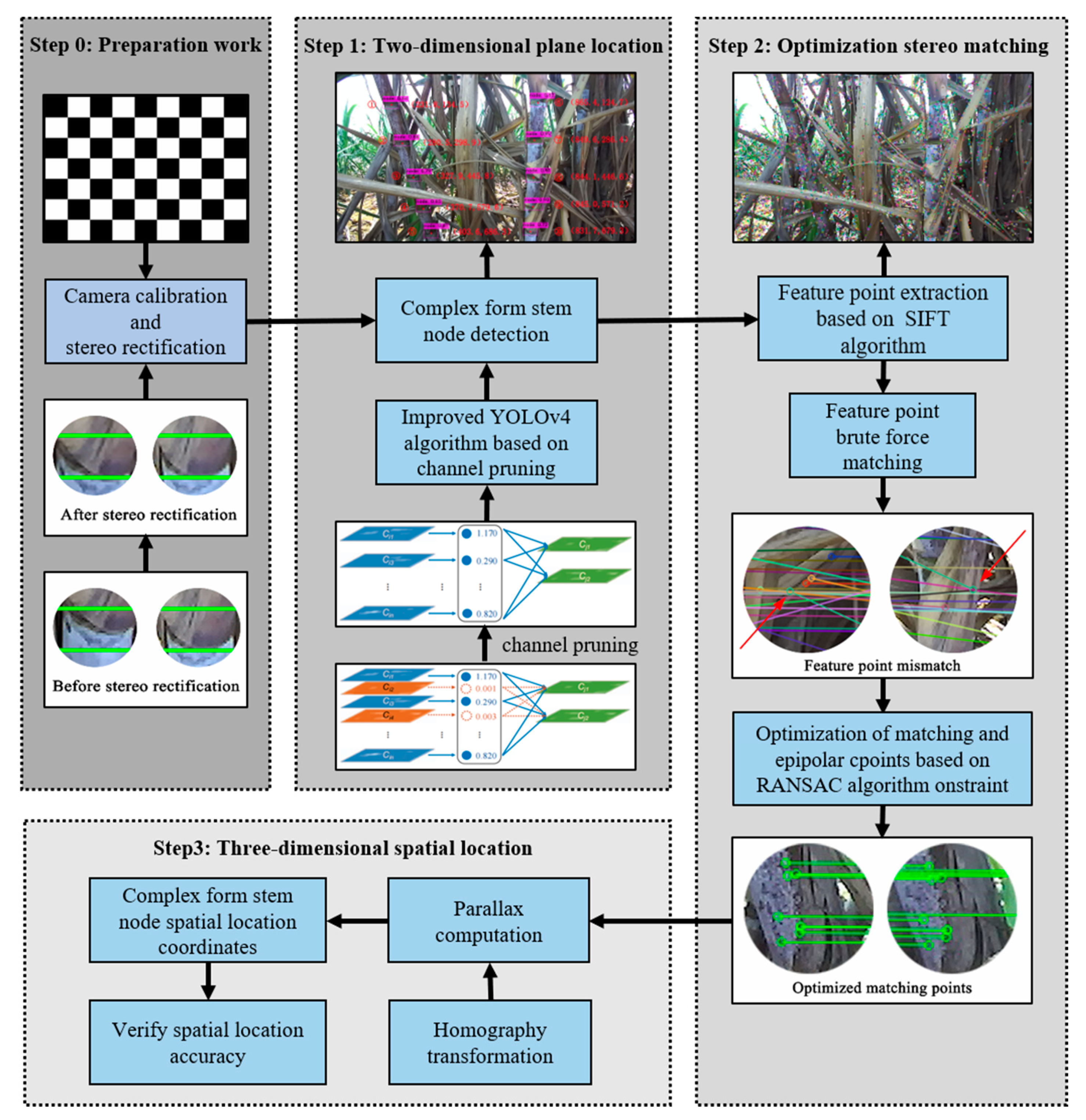
Figure 1 shows the systematic research route of the new binocular spatial location of sugarcane nodes based on the improved YOLOv4, which includes binocular camera calibration and stereo rectification to ensure the reliability of the hardware.
2.1. Binocular Stereo Vision Location Theory
2.1.1. Camera Imaging Model
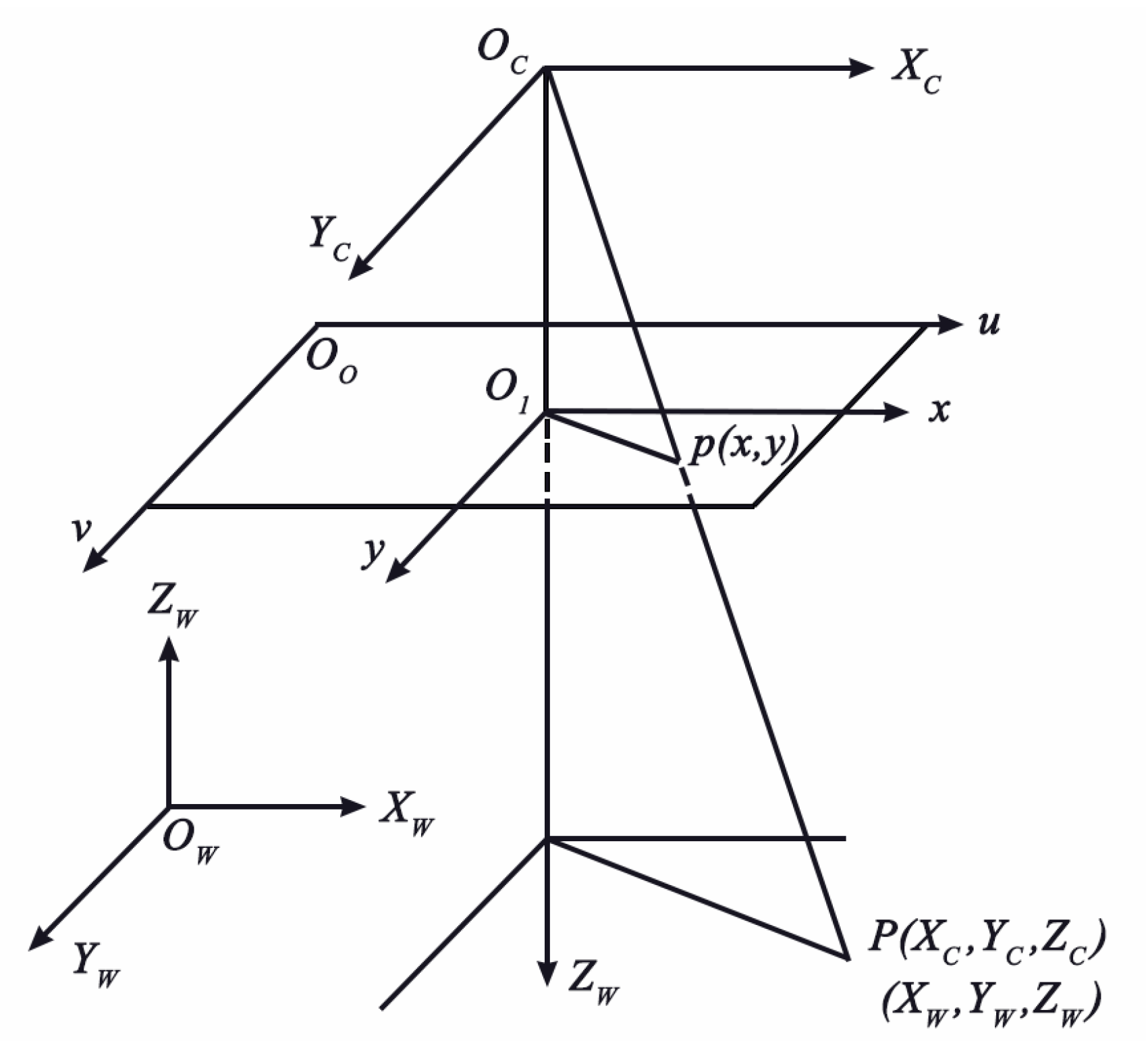
The camera imaging model describes the image formation of the geometric mathematical model transformation, and establishes the coordinate transformation relationship between the two-dimensional image plane and three-dimensional space. Camera imaging models are generally divided into linear models and nonlinear models, of which the most commonly used is the pinhole imaging model, a linear model [13]. In order to describe an object in the world coordinate system as an image in a plane two-dimensional image coordinate system, four coordinate systems of the pinhole imaging model need to be established to complete this transformation, which are the pixel coordinate system (O0-uv), image coordinate system (O1-xy), camera coordinate system (Oc-XcYcZc) and world coordinate system (Ow-XwYwZw), as shown in Figure 2.
For the ideal pinhole imaging model, the relationship between the world coordinate system and the pixel coordinate system can be established by mutual transformation of the four coordinate systems, as shown in Formula (1).
The four parameters fx, fy, u0 and v0 are internal parameters of the camera, which are determined by the internal structure of the camera when it was manufactured. Correspondingly, R and t are the external parameters of the camera. The internal and external parameters of the camera are all obtained by camera calibration. From Formula (1), if the internal parameter matrix M and the external parameter matrix N are known, the position (u, v) of any point in space with the coordinates (Xw, Yw, Zw, 1)T can be acquired in the image pixel coordinate system. However, since M is a 3 × 4 irreversible matrix, the position of the point (u, v) in the world coordinate system cannot be derived by its coordinates in the image pixel coordinate system. Hence, a stereo vision system is required.
2.1.2. Binocular Stereo Vision System Imaging Model
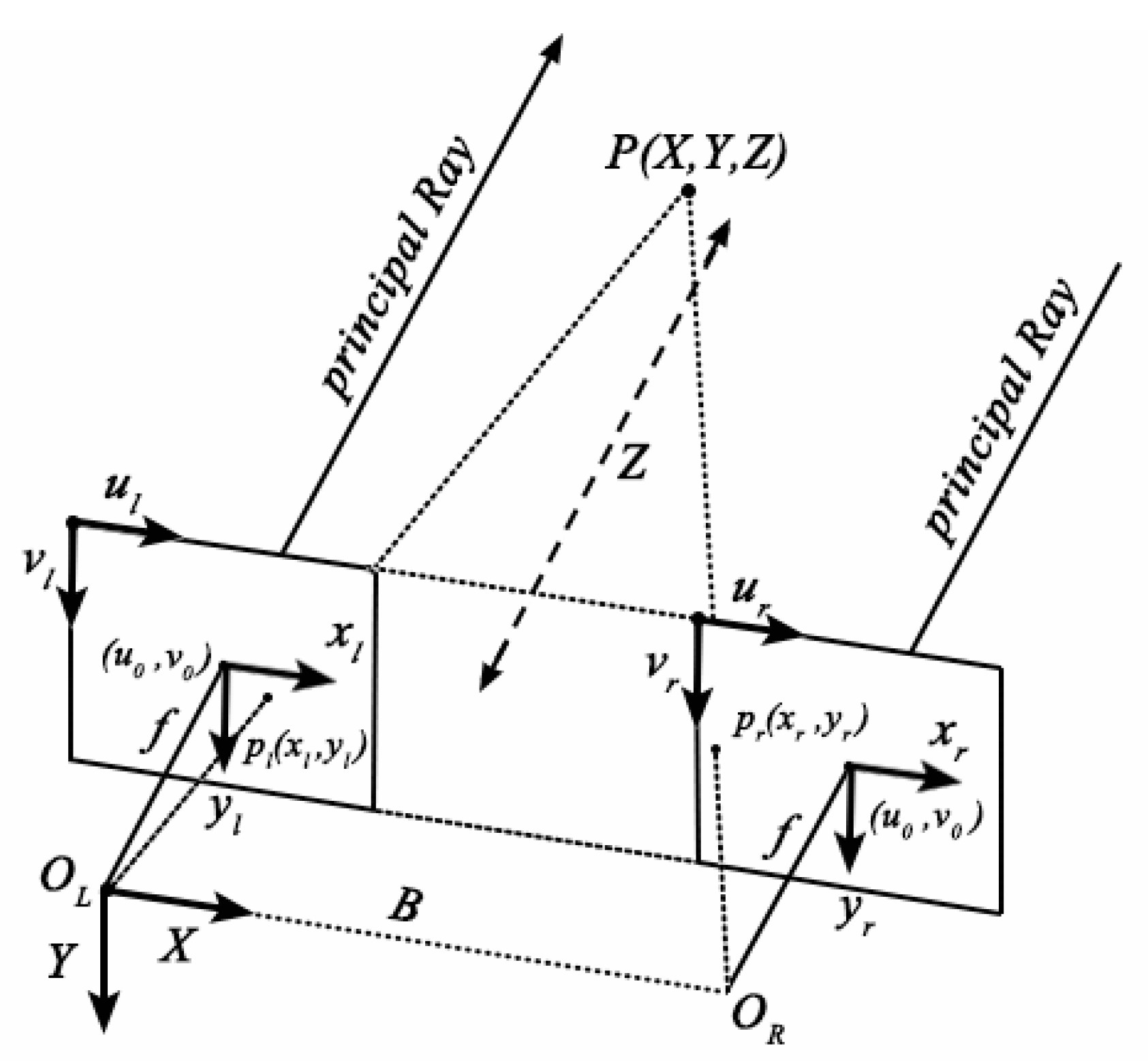
Binocular stereo vision [13] refers to using two cameras to film the same object from different angles; then, based on triangulation principle, the three-dimensional space position of the object is obtained by calculating the parallax, as shown in Figure 3.
In the parallel binocular vision model, the projection of any point in the camera coordinate system on the left and right camera planes is , , respectively. When , then according to the triangulation principle:
Furthermore:
where f is the focal length of the camera, and B is the baseline distance between the left and right cameras, both of which are fixed parameters of the camera. is the unknown parameter of the parallax. The object position in three-dimensional space can be restored only by calculating the parallax.
2.2. Calibration and Rectification of Binocular Camera
2.2.1. Calibration of Binocular Camera
The ZED2 binocular camera producing an RGB image with a resolution of 1280 × 720 pixels at 60 fps was used in this paper. Since the internal and external parameters of the camera are important for restoring 3D spatial location information, they can be obtained through the camera calibration. 30 pairs of pictures (60 images) with the calibration chessboard collected by a ZED2 binocular camera were put into the camera calibration box of MATLAB to calibrate the ZED2 binocular camera, as shown in Figure 4.
The camera parameters were calibrated by identifying the corners on the chessboard picture collected by the camera. After both cameras were calibrated, the calibration error was analysed by re-projecting the calibration results of the left and right cameras, respectively. The error analysis found that the errors of the left camera in the X and Y directions were 0.48406 and 0.39770 pixels, and the errors of the right camera in the X and Y directions were 0.4940 and 0.36554 pixels, which meet the accuracy requirements of the research. After calibrating the rotation matrix and translation matrix of the two cameras, the rotation matrix R was found to be similar to the identity matrix, which showed that the optical axes of the left and right cameras were nearly parallel. Meanwhile, the rotation angle between them was very small. The coordinate system was established by the optical centre position of the left camera as the origin, and the translation vector was acquired. This showed that the distance between the two cameras in the X-axis direction was 119.79 mm, which was very close to the given baseline length of 120 mm. At the same time, the deviation in the Y- and Z-axis directions was very small (0.138 mm and 0.504 mm, respectively). Through calibration, the camera was confirmed as meeting the needs of sugarcane location.
2.2.2. Stereo Rectification of Binocular Camera
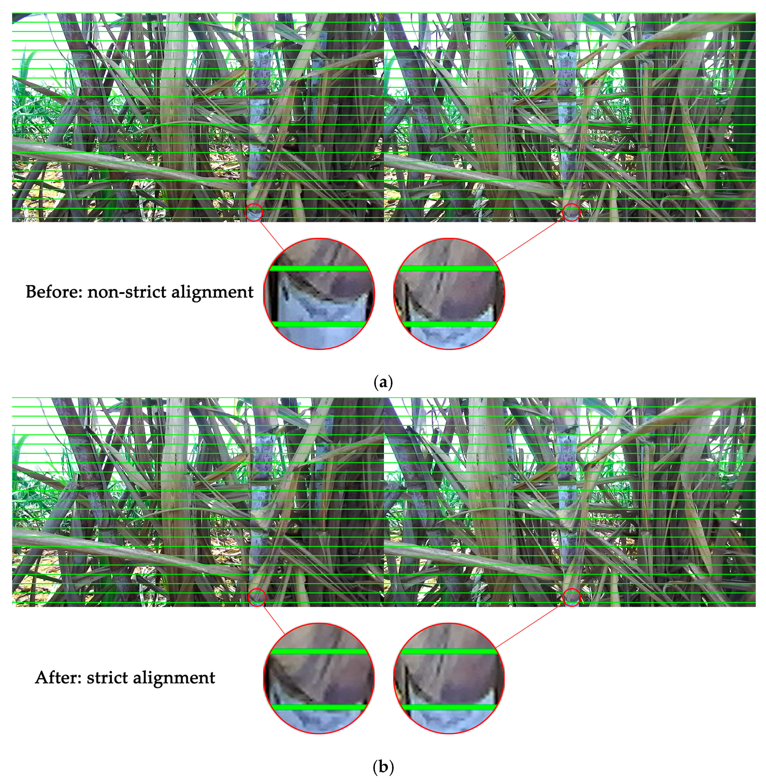
Ideally, the image planes of both cameras lie in the same plane. In this case, the pixels in the images taken by the left and right cameras are strictly aligned. However, the actual situation is more complicated. Due to the existence of errors, it is often necessary to mathematically correct the imaging plane of the camera to ensure the strict alignment of the pixels of the two images, which we call stereo rectification. In this study, the Bouguet stereo correction algorithm [14] was used to perform stereo rectification of the binocular cameras, and the camera parameters obtained from the previous calibration were imported into Visual Studio 2017, combined with the Opencv3.4.1 visual development library for stereo rectification. The binocular image pairs before and after stereo rectification are shown in Figure 5.
3. Methodology
3.1. YOLOv4 Model Improved by Channel Pruning Technology
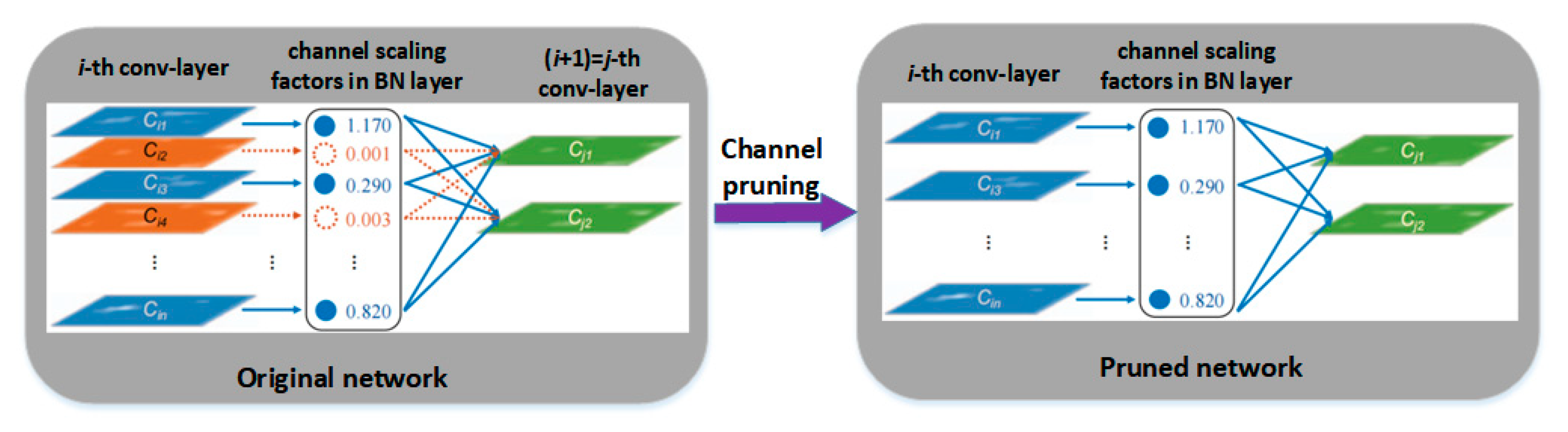
Previous research [9] by our team found that from comparative experiments of various target detection algorithms, YOLOv4 was the most suitable algorithm for detecting complex form stem nodes so far. However, the disadvantages of this algorithm are also obvious. It has a very complex network structure and a large number of network parameters, which requires high GPU processing power and is not suitable for transplanting to the embedded chip of a harvesting robot. Therefore, the model needs to be compressed. Channel Pruning Technology (CPT) [15] greatly reduces the size of the model but hardly affects the identification accuracy by means of eliminating the ineffective channels and their related inputs and outputs after identifying network channels. In this paper, the CPT was adopted to simplify the YOLOv4 algorithm model, and the Gamma (γ) coefficient of the Batch Normalization (BN) layer was selected as the evaluation index of the channel importance. According to the distribution of the γ coefficient and the pruning rate set by the optimal solution, the network channels of the algorithm were reduced by reserving the channels that played a greater role (blue part) and deleting the channels with γ coefficients approaching zero (orange part), as shown in Figure 6.
The experimental environment used in this improved experiment is as follows: Hardware: Intel Xeon Gold 5218 CPU @ 2.3 GHz processor, 64 GB memory; NVIDIA RTX 2080Ti GPU, 11 GB memory; Environment: CUDA10.2, cuDNN7.6.5, python3.6, pytorch1.8.1; Windows10 64 bit operating system.
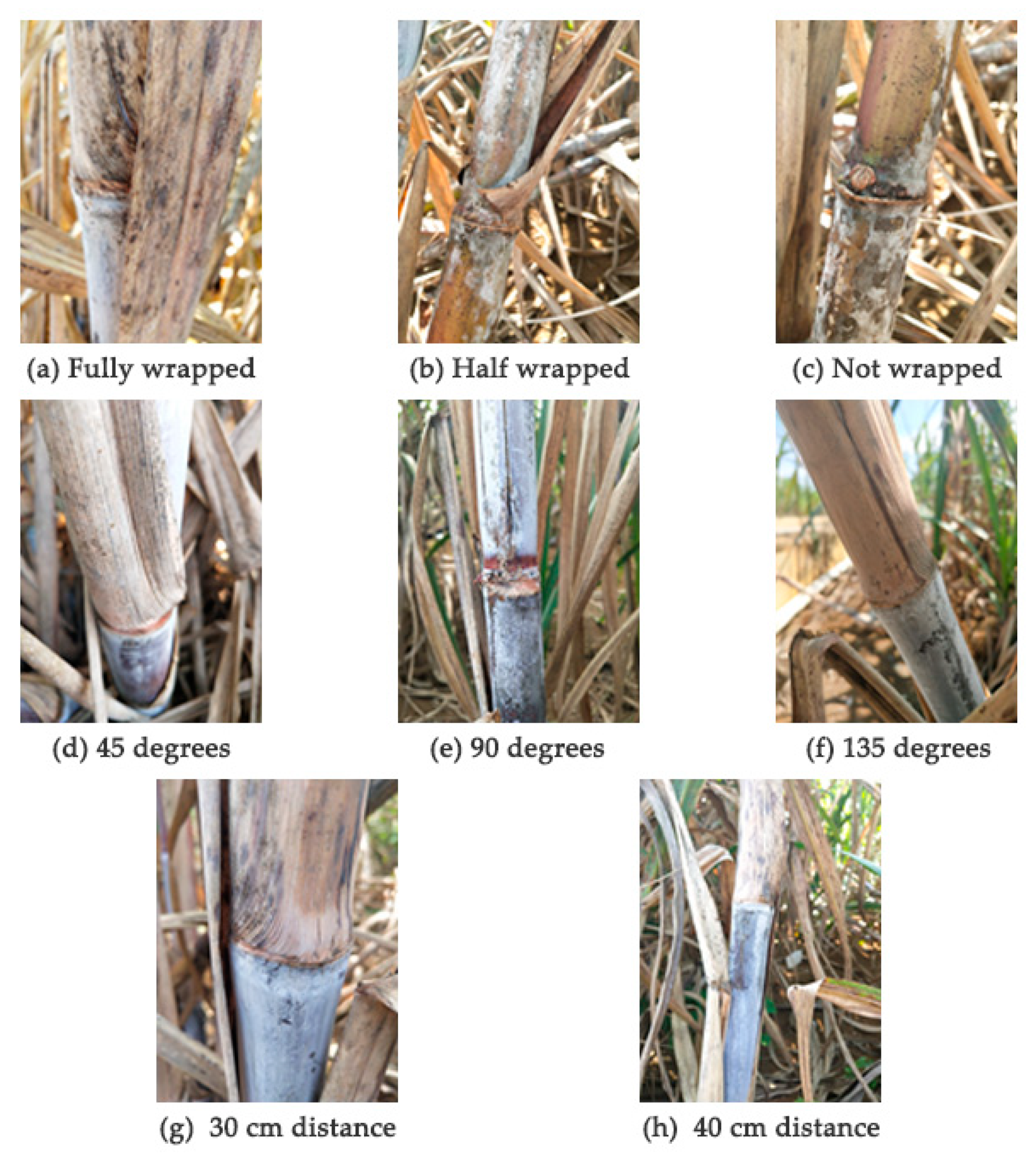
The dataset used in this improved experiment was sugarcane node images self-collected from the sugarcane planting base in Agricultural New Town, Guangxi University, China. The sugarcane variety was Guitang No. 49, and the average stem diameter was about 2.5 cm. To collect the complex field environment data, images of sugarcane nodes completely wrapped, half wrapped and unwrapped by sugarcane leaves from different angles and distances of the camera were collected at different time periods, as shown in Table 1. The stem node samples collected in different modes are shown in Figure 7.
At the same time, the samples were expanded by changing the saturation, sharpness, contrast and brightness of the images, and rotating them by 30 degrees. The dataset consisted of single sugarcane images with a single stem node, single sugarcane images with three stem nodes averagely and multiple sugarcane images with more than five stem nodes averagely. Finally, a dataset of 8000 images was obtained, of which 7200 were used as training sets and 800 as test sets. The method of the YOLOv4 model improved by CPT is as follows.
- (1)
- Normal training. A convergent and accurate YOLOv4 sugarcane node identification model is trained normally.
- (2)
- Sparse training. The L1 regularisation training is carried out on the BN layer of the normal training model, so that the γ coefficient of the BN layer is as close to 0 as possible, and the sparse weights are redistributed to other effective layers of the network.
- (3)
- Pruning. The channels in the BN layer with the γ coefficients approaching zero are picked out, and the channels are pruned according to the set pruning ratio to generate a simplified model that occupies less memory space.
- (4)
- Fine-tuning of the pruned model. All the BN layers are pruned at one time and then re-trained to fine-tune to overcome the decline of model accuracy after channel pruning.
The hyperparameters are the parameters set before training, seen in Table 2. In order to prevent over-fitting and under-fitting, they were optimized by Random Search (RS). Firstly, the selection range of each parameter was divided into several large intervals, and the parameter was randomly selected in each large interval. Secondly, the interval with the best training effect was selected, and further subdivided into several cells, before randomly selecting the parameter in small intervals. Finally, the above process was repeated until the optimal parameter combination was obtained. The main parameter settings of the experimental dataset modelling are shown in Table 2.
3.2. Identification of Sugarcane Nodes Based on Improved YOLOv4
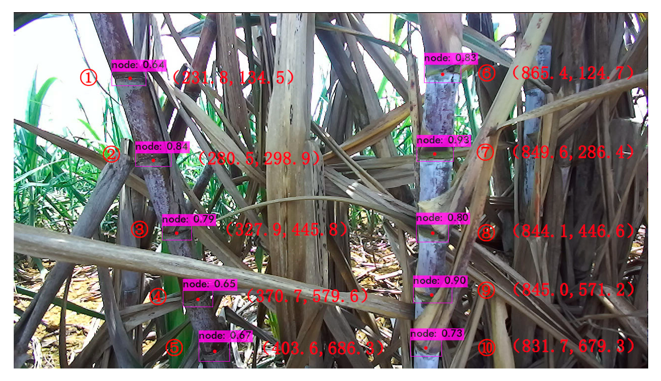
The weights file and the configuration file of the YOLOv4 model improved by Channel Pruning Technology were extracted and deployed to the embedded chip. The plane position of the stem nodes in the images collected by the left camera was identified and detected by the improved YOLOv4 algorithm. The centre point coordinates (x, y) of the stem node in the pixel coordinate system were also outputted. Furthermore, the detected stem nodes were labelled from top to bottom and left to right to verify the location accuracy, as shown in Figure 8.
3.3. Spatial Location of Sugarcane Nodes Based on Binocular Vision
3.3.1. Stereo Matching Based on SIFT Feature Points
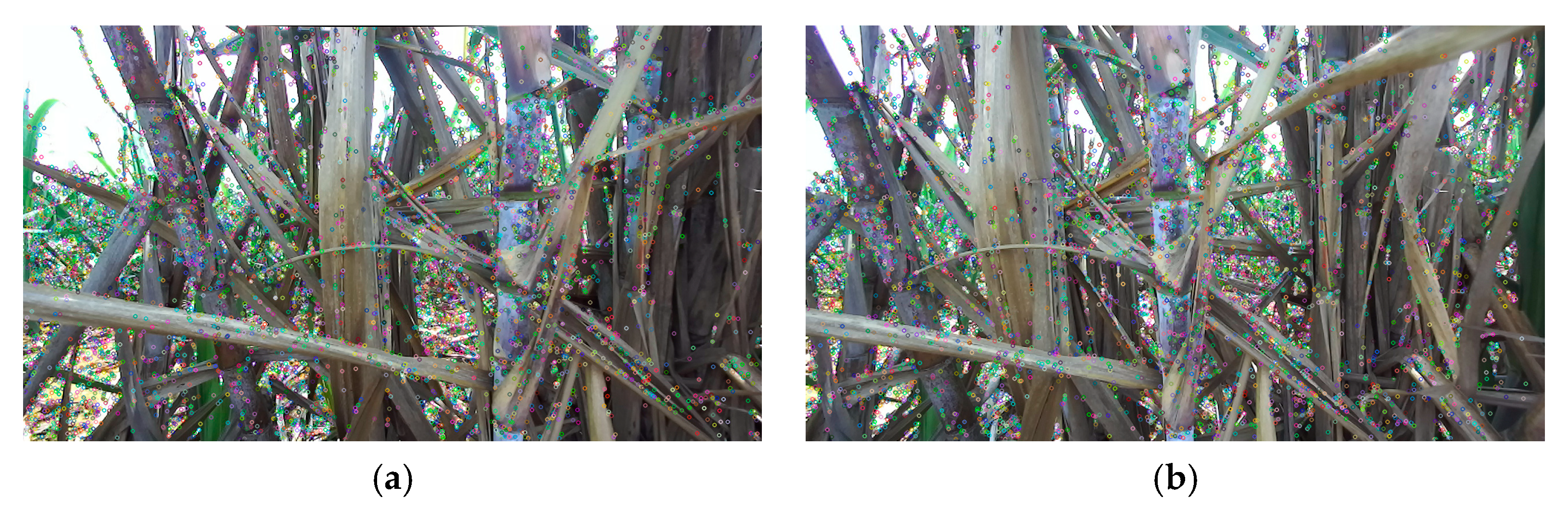
After the identification and plane location of the sugarcane nodes, we needed to locate the nodes in space. In the binocular stereo vision system, stereo matching is the most important step to get the spatial position information of objects. The stereo matching can find the correspondence of the same point in the two images taken by the left and right cameras. According to the different matching elements, stereo matching can be divided into matching algorithms based on the regional grey [16], the phase [17] and the features [18]. Due to the complex growing environment of sugarcane and frequent changes of field light, a feature-based matching algorithm that does not depend excessively on the image grey level and has good anti-interference performance against external factors is more suitable for the stereo matching of sugarcane nodes in this study. Scale-invariant feature transform (SIFT) [19] is a computer vision algorithm used to detect and describe local features in images by finding extreme points in spatial scales and extracting their position, scale and rotation invariants. It has good anti-interference performance against external light and noise. Figure 9 is the SIFT feature point extraction of the left and right cameras.
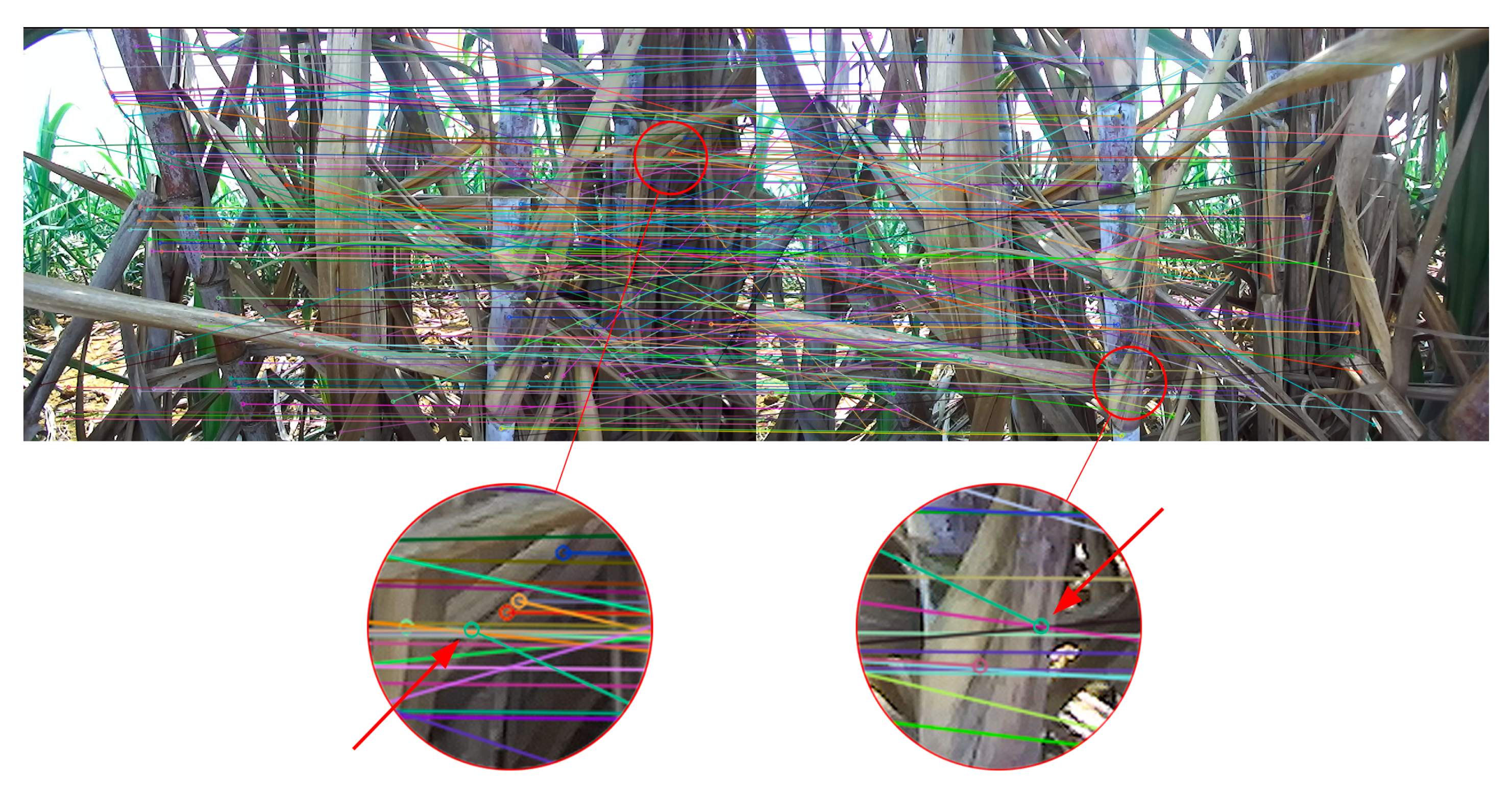
The extracted feature points of the left and right images must be matched one by one. However, stem nodes covered or shaded by leaves are too similar to other sugarcane leaves in the field, so the feature points are often mismatched, as shown in Figure 10.
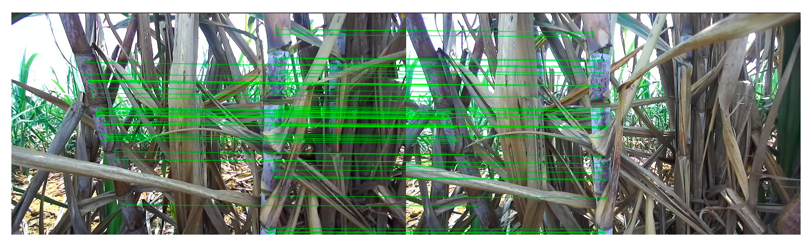
In order to improve the matching accuracy, the matching constraints were introduced to eliminate the wrongly matched pairs. Random sample consensus (RANSAC) [20] is an iterative algorithm to correctly estimate the parameters of a mathematical model from a set of data containing outliers. “Outliers” generally refer to the noise in the data, such as wrongly matched points in the above matching. Therefore, we can eliminate these by introducing the RANSAC algorithm. On the other hand, after stereo correction, we have aligned the row pixels of the left and right images. Moreover, we can use the epipolar constraint whereby the connection between matching point pairs can only be a specific straight line in order to eliminate feature point pairs with inconsistent pixels in the right row of the left and right images. With the introduction of the RANSAC algorithm and the epipolar constraint, the mismatch problem has been basically solved, as shown in Figure 11.
3.3.2. Solution of Homography Matrix H
In order to obtain the three-dimensional coordinates of sugarcane nodes, it is necessary to know the parallax of the nodes in the left and right camera images, which is the difference in values between the X coordinates of the nodes in the left and right camera image coordinate systems. The homography matrix H [21] reflects the mapping relationship of corresponding points between the left camera image and the right camera image in the binocular camera. It can be obtained through the optimised stereo matching feature points. Assuming a pair of optimised matching feature points, the pixel coordinate in the left camera image is , its corresponding point in the right camera image is , and the homography matrix is H, then:
The above formula is expanded as follows:
Substituting the third equation in Equation (5) into the first two equations, there are eight unknown parameters in matrix H, in which s is the scale factor (s ≠ 0). Because each pair of matching points can provide two equations, the homography matrix H can be obtained by only four pairs of matching points. Since the optimised pairs of matching points in our stereo matching experiment above are far more than four pairs, this is enough to solve the homography matrix H. In order to improve the robustness, the RANSAC algorithm is introduced into the process of solving the homography matrix, so as to achieve the optimal correspondence matrix H.
3.3.3. Spatial Location of Sugarcane Nodes
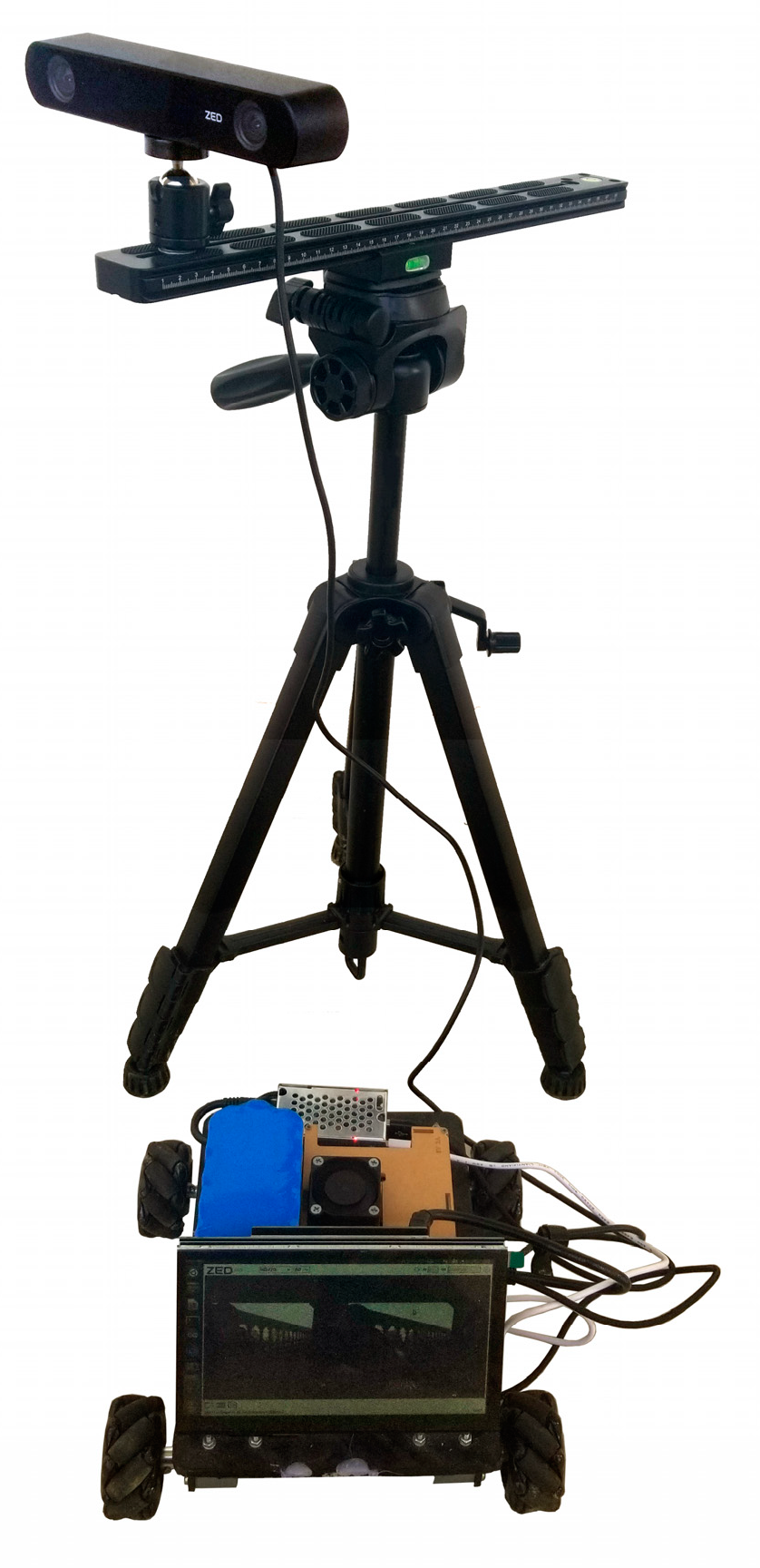
The centre point coordinates of the stem node in the left camera detected by the improved YOLOv4 algorithm are recorded as . The corresponding point in the right picture was obtained by putting into Formula (5), then the parallax . Finally, the three-dimensional spatial coordinates of the stem node can be acquired by Formula (3). Because the most important index to evaluate the reliability of a binocular vision system is the accuracy of the coordinate in the Z-axis under spatial location, the left camera coordinate system was selected as the world coordinate system to verify the accuracy of the coordinates in the Z-axis under spatial location. Figure 12 shows the experimental platform of the spatial location of the binocular camera. The ZED2 binocular camera was used for image acquisition, and NVIDIA Jetson Nano was applied as an embedded chip for data processing, which communicate with each other through USB3.0. The overall platform was equipped with a camera-moving guide with a precise scale, as well as a power supply, screen and other related accessories.
Due to the difficulty in accurately measuring the distance from each node to the XOY plane of the left camera coordinate system, the relative distance was used to measure the location accuracy of the coordinate in the Z-axis. The experimental process was as follows:
- (1)
- The binocular camera was fixed on the bracket guide rail with a scale, and the position of the guide rail where the camera was currently located was recorded. Subsequently, the sugarcane images in the field were collected and the spatial location experiment was carried out according to the method mentioned above. After sampling three times, the average XYZ coordinates of each node were recorded as the coordinates before moving. At the same time, the time spent in each location experiment was recorded.
- (2)
- The position of the binocular camera in the X and Y directions was kept unchanged, the camera was moved on the guide rail in the Z direction by D = 100 mm, the spatial location experiment was conducted again, and the average xyz coordinates of each node were recorded as the moved coordinates. In addition, the time required for each location experiment was recorded again.
- (3)
- The Z coordinate was subtracted before and after moving to get the average distance difference of two positions, and finally D was subtracted from the difference to get the location error in the Z coordinate.
4. Results and Discussion
4.1. Target Detection Results of YOLOv4 Improved by Channel Pruning Technology
The loss function of the model after sparse training in Section 3.1 is shown in Formula (6):
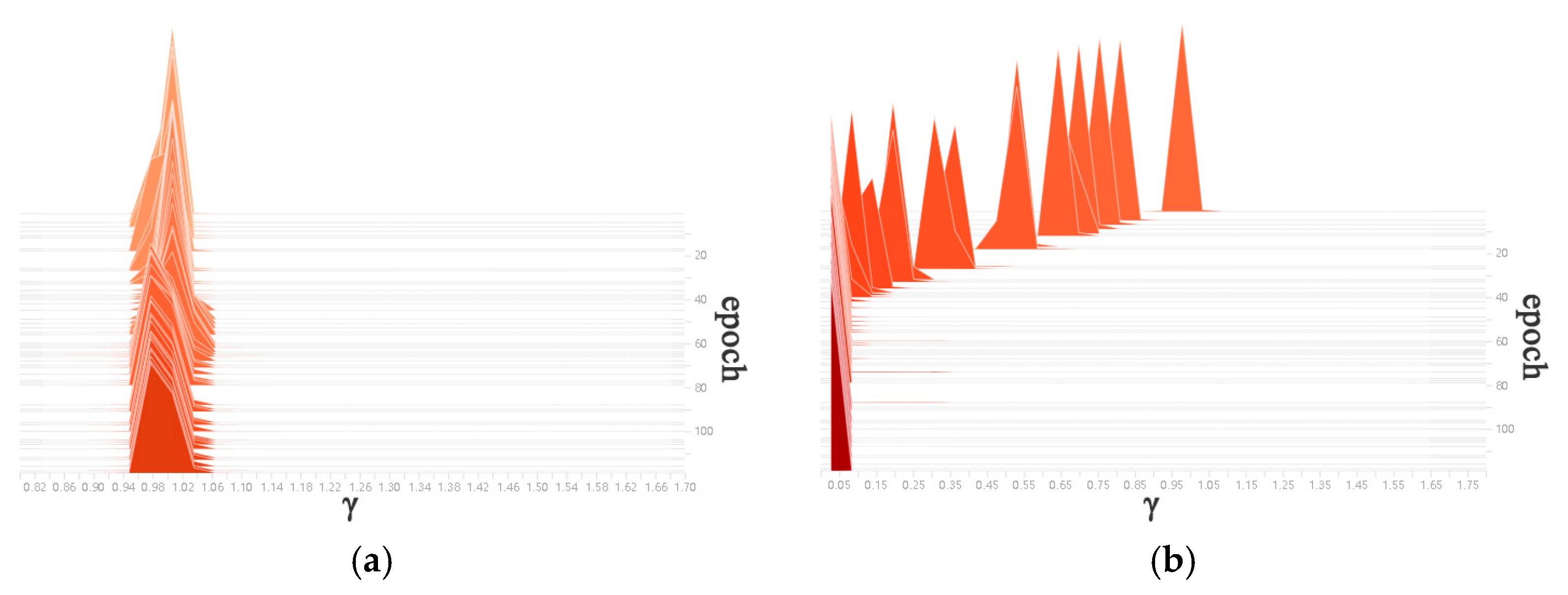
is the training loss of the network, x and y are the input and output of model training, respectively, and W is the training parameter in the network. is the L1 regular constraint term of the γ coefficient of the BN layer, and λ is the penalty factor. The distribution diagram of the γ coefficient of the BN layer during normal training is shown in Figure 13a, and was mainly distributed around 1. The distribution diagram of the γ coefficients of the BN layer during the sparse training is shown in Figure 13b. In the sparse training process, as the number of epochs increased, the γ coefficient of the BN layer gradually approached zero, which indicated that the γ coefficient gradually became sparse. By the 120th epoch, the sparsity change gradually became weak, and the sparsity training was saturated.
Five commonly used indicators, average precision (AP), Params, Floating Point operations (FLOPs), model size and speed, were used to verify the performance of the improved model. The definition of average precision (AP) is shown in Formula (7), where P(r) represents a PR curve with precision (P) as the horizontal axis and recall (R) as the vertical axis:
The Params and Floating Point operations (FLOPs) are defined as shown in Formulas (8) and (9), where H and W represent the width and height of the input image, K is the convolution kernel size, and Cin and Cout represent the number of convolution kernels input and output.
On the premise that the accuracy was not reduced greatly, 0.6 was selected as the pruning rate to shrink the YOLOv4 target detection model after sparse training. Finally, the Params, FLOPs and model size were all decreased by about 89.1% after 19,331 channels were cut off, while the average precision (AP) decreased by only 0.1% (from 94.5% to 94.4%). To be specific, the Params decreased from 63,937,686 to 6,973,211, the FLOPs decreased from 29.88 G to 3.26 G, and the model size decreased from 244 M to 26.7 M, which indicated that the pruned model was much smaller than the original one and the improved algorithm was successful.
4.2. Comparison between Improved YOLOv4 and Other Target Detection Algorithms
Three target detection algorithms that are often used in crop identification were selected to further verify the effectiveness and superiority of the improved algorithm. The self-collected data sets of stem nodes in the wild field environment were used to test and evaluate their performance, as shown in Table 3. In order to ensure robustness, we have conducted several experiments, but we found that there was almost no difference in the results of each performance evaluation experiment. The following, main reasons might explain why this is the case. First of all, the training set and test set was the same dataset to verify the performance of each algorithm, which can greatly reduce the randomness of the results. Secondly, the above-mentioned deep learning algorithm ensures a fair degree of robustness through the large amount of data, and the error can be corrected within the neural network. Finally, because the recognition object of this paper is only a single target, which greatly reduces the difficulty of recognition, the difference between each experiment is very small. Therefore, under the condition of the same experimental hyperparameter settings, the differences between the repeated experiments were inconsiderable.
From Table 3, the improved YOLOv4 algorithm had the strongest comprehensive performance among the four algorithms. In terms of average precision (AP), the improved YOLOv4 model was 1.3% and 0.3% higher than SSD and YOLOv3, and only 0.1% lower than before the improvement. However, in terms of the Params, FLOPs and model size, the improved YOLOv4 algorithm was only about 1/3 of SSD and 1/10 of YOLOv3 and YOLOv4. The comparison of results adequately illustrated the superiority of the improved YOLOv4 algorithm model.
4.3. Analysis of Spatial Location Accuracy of Sugarcane Nodes
In Figure 7, the three-dimensional spatial coordinates of each sugarcane node were calculated by Formula (3). Now the spatial location coordinate and its accuracy are shown in Table 4.
According to Table 4, the maximum and minimum errors of the Z coordinate of the sugarcane node spatial location were 2.86 mm and 1.13 mm, and the average error was 1.88 mm. It should be noted that the position of the XOY plane will have a slight deviation with the movement, which is reflected in the slight coordinate difference in the X- and Y-axis before and after moving.
4.4. Real-Time Performance of the Proposed Method
Although the training time of the improved YOLOv4 model was about 14 h, the time for identifying stem nodes with the improved model was very short. By program statistics, the total execution time spent in the sugarcane stem node spatial location is shown in Table 5. The extraction and matching of feature points and the subsequent elimination of mismatching points occupied most of the time by the proposed method. It should be noted that the other time in Table 5 refers to the time for feature point extraction and matching and the subsequent elimination of mismatching points. Additionally, the before (after) move- 1/2/3 refers to the three location experiments before (after) the camera moves D = 100 mm in the verification experiment of stem node location accuracy.
4.5. Location Methods Comparison and Discussion
The new binocular location method based on improved YOLOv4 proposed in this paper not only successfully solved the difficult problem of stem node location, but also achieved better results in location accuracy than traditional crop location methods. For example, Xiong et al. [25] proposed a binocular vision method for picking point positioning of disturbance litchi cluster, and the H component of litchi image was directly used for stereo matching. This method does not extract and optimize feature points as present in this paper, resulting in the maximum location error of 58 mm in Z direction. Xie et al. [26] identified the position of beef tomato based on R-CNN and binocular imaging technology. It directly used the SDK of the binocular camera to measure the distance without considering the targeted improvement for the location object, which led to a large number of mismatches. Therefore, the maximum location error of its Z axis was 18.6 mm, which was not ideal for small crops location. Luo et al. [27] obtained the position information of grape clusters based on the dense disparity calculation method of gray value matching, and finally the maximum location error of Z axis was 12 mm. Because the gray value might be affected by illumination, the location accuracy based on the matching method of gray value was lower than that of the feature point-based. In the previous finding of Wang et al. [28], which used two CCD color cameras integrated with a window zooming-based algorithm to locate multiple fruits and vegetables, results showed that the maximum Z-axis location error was 7.5 mm. On the contrary, the maximum Z-axis location error of the method proposed in this paper was only 2.86 mm, which was far lower than the location methods in the above-mentioned literatures. This fully demonstrates the superiority of the method proposed in this paper. The main reason that this might be applied is because the improved YOLOv4 algorithm can still keep high accuracy with greatly reduced complexity. At the same time, a large number of mismatching points are eliminated by RANSAC algorithm and epipolar constraint, thus further improving the location accuracy.
5. Conclusions
In this paper, a new binocular location method based on an improved YOLOv4 was proposed to solve the problem of the difficulty of sugarcane nodes spatial location due to the complex form characteristics in the field environment and the high demand for computational capability.
- (1)
- The deep learning algorithm of YOLOv4 was improved by the Channel Pruning Technology in network slimming, so as to ensure the high recognition accuracy of the deep learning algorithm and to facilitate transplantation to embedded chips. The experimental results showed that the Params, FLOPs and model size were all reduced by about 89.1%, while the average precision (AP) decreased by only 0.1% (from 94.5% to 94.4%). To be specific, the Params decreased from 63,937,686 to 6,973,211, the FLOPs decreased from 29.88 G to 3.26 G, and the model size decreased from 244 M to 26.7 M, which greatly reduced the computational demand.
- (2)
- Compared with other deep learning algorithms, the improved YOLOv4 algorithm also has great advantages. Specifically, the improved algorithm was 1.3% and 0.3% higher than SSD and YOLOv3 in average precision (AP). In terms of parameters, FLOPs and model size, the improved YOLOv4 algorithm was only about 1/3 of SSD and 1/10 of YOLOv3. The above data sufficiently demonstrated the superiority of the improved YOLOv4 algorithm model.
- (3)
- The SIFT algorithm, with its strong anti-light interference ability, was used to extract feature points from complex form sugarcane pictures. Furthermore, the SIFT feature points were optimised by the RANSAC algorithm and epipolar constraint, which effectively reduced the mismatching problem caused by the similarity between stem nodes and sugarcane leaves.
- (4)
- The optimised matching point pairs were used to solve the homography transformation matrix, so as to obtain the three-dimensional spatial coordinates of the complex form stem nodes and verify their spatial location accuracy. The experimental results showed that the maximum error of the Z coordinate in the spatial location of complex form stem nodes was 2.86 mm, the minimum error was 1.13 mm, and the average error was 1.88 mm, which totally meet the demand of sugarcane harvesting robots in the next stage.
Considering the requirements for extended application on extreme environments, further research investigating effects of the stem node recognition and location on the night time with supplementary light may be beneficial. The parameters of the supplementary lights, including the angle of supplementary lights, the number of lights, the change of illuminance and the interference of surrounding light source, are worth being discussed.
Author Contributions
Conceptualization, C.Z.; methodology, C.Z.; software, C.Z.; validation, S.H., H.G., Y.L. and C.W.; formal analysis, C.Z. and Y.L.; investigation, C.Z. and S.H.; resources, S.H., Y.L. and H.G.; data curation, C.Z.; writing—original draft preparation, C.Z.; writing—review and editing, S.H., Y.L. and C.W.; visualization, C.Z.; supervision, S.H. and H.G.; project administration, S.H. and H.G.; funding acquisition, S.H., Y.L. and H.G. All authors have read and agreed to the published version of the manuscript.
Funding
This study was supported by the National Nature Science Foundation of China (No. 51965004).
Institutional Review Board Statement
Not applicable.
Informed Consent Statement
Not applicable.
Data Availability Statement
Not applicable.
Acknowledgments
The authors would like to thank Wen Chen for his contribution to this article, and thank Kang Yu, Yonggang Huang and Shun’an Lai for their contributions to data set labeling.
Conflicts of Interest
The authors declare that the research was conducted in the absence of any commercial or financial relationships that could be construed as a potential conflict of interest.
References
- Silwal, A.; Davidson, J.R.; Karkee, M.; Mo, C.; Zhang, Q.; Lewis, K. Design, integration, and field evaluation of a robotic apple harvester. J. Field Robot. 2017, 34, 1140–1159. [Google Scholar] [CrossRef]
- Zhang, B.; Huang, W.; Wang, C.; Gong, L.; Zhao, C.; Liu, C.; Huang, D. Computer vision recognition of stem and calyx in apples using near-infrared linear-array structured light and 3D reconstruction. Biosyst. Eng. 2015, 139, 25–34. [Google Scholar] [CrossRef]
- Williams, H.A.; Jones, M.H.; Nejati, M.; Seabright, M.J.; Bell, J.; Penhall, N.D.; Barnett, J.J.; Duke, M.D.; Scarfe, A.J.; Ahn, H.S. Robotic kiwifruit harvesting using machine vision, convolutional neural networks, and robotic arms. Biosyst. Eng. 2019, 181, 140–156. [Google Scholar] [CrossRef]
- Ling, X.; Zhao, Y.; Gong, L.; Liu, C.; Wang, T. Dual-arm cooperation and implementing for robotic harvesting tomato using binocular vision. Robot. Auton. Syst. 2019, 114, 134–143. [Google Scholar] [CrossRef]
- Li, J.; Tang, Y.; Zou, X.; Lin, G.; Wang, H. Detection of fruit-bearing branches and localization of litchi clusters for vision-based harvesting robots. IEEE Access 2020, 8, 117746–117758. [Google Scholar] [CrossRef]
- Meng, Y.; Ye, C.; Yu, S.; Qin, J.; Zhang, J.; Shen, D. Sugarcane node recognition technology based on wavelet analysis. Comput. Electron. Agric. 2019, 158, 68–78. [Google Scholar] [CrossRef]
- Chen, J.; Wu, J.; Qiang, H.; Zhou, B.; Xu, G.; Wang, Z. Sugarcane nodes identification algorithm based on sum of local pixel of minimum points of vertical projection function. Comput. Electron. Agric. 2021, 182, 105994. [Google Scholar] [CrossRef]
- Lu, S.; Wen, Y.; Ge, W.; Peng, H. Recognition and features extraction of sugarcane nodes based on machine vision. Trans. Chin. Soc. Agric. Mach. 2010, 41, 190–194. [Google Scholar]
- Chen, W.; Ju, C.; Li, Y.; Hu, S.; Qiao, X. Sugarcane stem node recognition in field by deep learning combining data expansion. Appl. Sci. 2021, 11, 8663. [Google Scholar] [CrossRef]
- Bochkovskiy, A.; Wang, C.; Liao, H.M. YOLOv4: Optimal speed and accuracy of object detection. arXiv 2020, arXiv:2004.10934. [Google Scholar]
- Suo, R.; Gao, F.; Zhou, Z.; Fu, L.; Song, Z.; Dhupia, J.; Li, R.; Cui, Y. Improved multi-classes kiwifruit detection in orchard to avoid collisions during robotic picking. Comput. Electron. Agric. 2021, 182, 106052. [Google Scholar] [CrossRef]
- Liu, G.; Nouaze, J.C.; Touko Mbouembe, P.L.; Kim, J.H. YOLO-tomato: A robust algorithm for tomato detection based on YOLOv3. Sensors 2020, 20, 2145. [Google Scholar] [CrossRef] [PubMed] [Green Version]
- Yang, L.; Wang, B.; Zhang, R.; Zhou, H.; Wang, R. Analysis on location accuracy for the binocular stereo vision system. IEEE Photonics J. 2017, 10, 7800316. [Google Scholar] [CrossRef]
- Bouguet, J. Camera Calibration Toolbox for Matlab. 2004. Available online: http://www.vision.caltech.edu/bouguetj/calib_doc/index.html (accessed on 19 January 2022).
- Liu, Z.; Li, J.; Shen, Z.; Huang, G.; Yan, S.; Zhang, C. Learning efficient convolutional networks through network slimming. In Proceedings of the IEEE International Conference on Computer Vision, Venice, Italy, 22–29 October 2017. [Google Scholar]
- Wang, Z.; Zheng, Z. A region based stereo matching algorithm using cooperative optimization. In Proceedings of the 2008 IEEE Conference on Computer Vision and Pattern Recognition, Anchorage, AK, USA, 23–28 June 2008. [Google Scholar]
- Zhao, H.; Wang, Z.; Jiang, H.; Xu, Y.; Dong, C. Calibration for stereo vision system based on phase matching and bundle adjustment algorithm. Opt. Laser. Eng. 2015, 68, 203–213. [Google Scholar] [CrossRef]
- Birinci, M.; Diaz-De-Maria, F.; Abdollahian, G.; Delp, E.J.; Gabbouj, M. Neighborhood matching for object recognition algorithms based on local image features. In Proceedings of the 2011 Digital Signal Processing and Signal Processing Education Meeting (DSP/SPE), Sedona, AZ, USA, 4–7 January 2011. [Google Scholar]
- Lowe, D.G. Distinctive image features from scale-invariant keypoints. Int. J. Comput. Vision 2004, 60, 91–110. [Google Scholar] [CrossRef]
- Fischler, M.A.; Bolles, R.C. Random sample consensus: A paradigm for model fitting with applications to image analysis and automated cartography. Commun. ACM 1981, 24, 381–395. [Google Scholar] [CrossRef]
- Barath, D.; Kukelova, Z. Homography from two orientation-and scale-covariant features. In Proceedings of the 2019 IEEE/CVF International Conference on Computer Vision, Seoul, Korea, 27–28 October 2019. [Google Scholar]
- Peng, H.; Huang, B.; Shao, Y.; Li, Z.; Zhang, C.; Chen, Y.; Xiong, J. General improved SSD model for picking object recognition of multiple fruits in natural environment. Trans. Chin. Soc. Agric. Eng. 2018, 34, 155–162. [Google Scholar]
- Jing, L.; Wang, R.; Liu, H.; Shen, Y. Orchard pedestrian detection and location based on binocular camera and improved YOLOv3 algorithm. Trans. Chin. Soc. Agric. Eng. Mach. 2020, 51, 34–39. [Google Scholar]
- Yuan, W.; Choi, D. UAV-based heating requirement determination for frost management in apple orchard. Remote Sens. 2021, 13, 273. [Google Scholar] [CrossRef]
- Xiong, J.; He, Z.; Lin, R.; Liu, Z.; Bu, R.; Yang, Z.; Peng, H.; Zou, X. Visual positioning technology of picking robots for dynamic litchi clusters with disturbance. Comput. Electron. Agric. 2018, 151, 226–237. [Google Scholar] [CrossRef]
- Hsieh, K.; Huang, B.; Hsiao, K.; Tuan, Y.; Shih, F.; Hsieh, L.; Chen, S.; Yang, I. Fruit maturity and location identification of beef tomato using R-CNN and binocular imaging technology. J. Food Meas. Charact. 2021, 15, 5170–5180. [Google Scholar] [CrossRef]
- Luo, L.; Tang, Y.; Zou, X.; Ye, M.; Feng, W.; Li, G. Vision-based extraction of spatial information in grape clusters for harvesting robots. Biosyst. Eng. 2016, 151, 90–104. [Google Scholar] [CrossRef]
- Wang, C.; Luo, T.; Zhao, L.; Tang, Y.; Zou, X. Window zooming–based localization algorithm of fruit and vegetable for harvesting robot. IEEE Access 2019, 7, 103639–103649. [Google Scholar] [CrossRef]
Figure 1.
The systematic research route of the new binocular spatial location of sugarcane nodes based on the improved YOLOv4.
Figure 1.
The systematic research route of the new binocular spatial location of sugarcane nodes based on the improved YOLOv4.

Figure 2.
Four coordinate systems in the pinhole imaging model.

Figure 3.
Binocular stereo vision imaging model.

Figure 4.
Image pairs used in binocular camera calibration. (a) Image taken by left camera. (b) Image taken by right camera.
Figure 4.
Image pairs used in binocular camera calibration. (a) Image taken by left camera. (b) Image taken by right camera.

Figure 5.
Binocular image pairs before and after stereo rectification. (a) Binocular image pairs before stereo rectification. (b) Binocular image pairs after stereo rectification.
Figure 5.
Binocular image pairs before and after stereo rectification. (a) Binocular image pairs before stereo rectification. (b) Binocular image pairs after stereo rectification.

Figure 6.
The process of channel pruning in this paper.

Figure 7.
The stem node samples collected in different modes.

Figure 8.
Sugarcane nodes identification and plane position detection based on improved YOLOv4.

Figure 9.
SIFT feature point extraction effect of image collected by left and right cameras. (a) left camera. (b) right camera.
Figure 9.
SIFT feature point extraction effect of image collected by left and right cameras. (a) left camera. (b) right camera.

Figure 10.
Schematic diagram of feature point error matching.

Figure 11.
Feature point match map optimised based on RANSAC algorithm and epipolar constraint.

Figure 12.
Experimental platform of the spatial location of binocular camera.

Figure 13.
Distribution diagram of γ coefficient of BN layer. (a) Normal training epochs. (b) Sparse training epochs.
Figure 13.
Distribution diagram of γ coefficient of BN layer. (a) Normal training epochs. (b) Sparse training epochs.


Table 1.
Data collection of stem nodes in a complex field environment.
| Time | Fully Wrapped | Half Wrapped | Not Wrapped | 45 Degrees | 90 Degrees | 135 Degrees | 30 cm Distance | 40 cm Distance | Total |
|---|---|---|---|---|---|---|---|---|---|
| 08:00 a.m. | 50 | 50 | 50 | 50 | 50 | 50 | 50 | 50 | 400 |
| 13:00 p.m. | 100 | 100 | 100 | 100 | 100 | 100 | 100 | 100 | 800 |
| 18:00 p.m. | 50 | 50 | 50 | 50 | 50 | 50 | 50 | 50 | 400 |
Table 2.
The main parameter settings of the experimental dataset modelling.
| Stage | Parameter Name | Parameter Value |
|---|---|---|
| Sparse training | Training batch size | 8 |
| Learning rate | 0.002 | |
| Epoch | 120 | |
| Sparseness rate | 0.001 | |
| Channel pruning | Pruning rate | 0.6 |
| Fine-tune model | Epoch | 120 |
| Training batch size | 8 |
Table 3.
Comparison of improved YOLOv4 algorithm with SSD, YOLOv3 and YOLOv4 algorithm.
| Algorithm | AP (%) | Params | FLOPs | Model Size | Speed (s) |
|---|---|---|---|---|---|
| SSD [22] | 93.1 | 23,612,246 | 30.44 G | 90.5 M | 0.023 |
| YOLOv3 [23] | 94.1 | 61,523,734 | 32.76 G | 235 M | 0.042 |
| YOLOv4 [24] | 94.5 | 63,937,686 | 29.88 G | 244 M | 0.035 |
| Pruned YOLOv4 | 94.4 | 6,973,211 | 3.26 G | 26.7 M | 0.032 |
Table 4.
The spatial location coordinate and its accuracy of sugarcane nodes.
| Node Number | Coordinate before Move (mm) | Coordinate after Move (mm) | Z-Coordinate D-Value (mm) | Actual D-Value (mm) | Z-Coordinate Error (mm) |
|---|---|---|---|---|---|
| 1 | (−237.98, 131.46, 370.52) | (−236.26, 133.02, 468.25) | 97.73 | 100 | −2.27 |
| 2 | (−209.58, 35.62, 382.81) | (−208.17, 36.94, 481.17) | 98.36 | 100 | −1.64 |
| 3 | (−181.95, −50.02, 403.56) | (−179.97, −48.98, 502.43) | 98.87 | 100 | −1.13 |
| 4 | (−157.01, −128.03, 422.13) | (−155.64, −126.08, 520.72) | 98.59 | 100 | −1.41 |
| 5 | (−137.82, −190.23, 438.76) | (−136.56, −189.20, 536.67) | 97.91 | 100 | −2.09 |
| 6 | (131.41, 137.18, 273.34) | (133.42, 138.83, 371.46) | 98.12 | 100 | −1.88 |
| 7 | (122.20, 42.91, 288.73) | (123.62, 44.29, 386.64) | 97.91 | 100 | −2.09 |
| 8 | (118.98, −50.49, 302.48) | (119.48, −49.21, 401.29) | 98.81 | 100 | −1.19 |
| 9 | (119.52, −123.13, 320.42) | (120.98, −121.68, 418.16) | 97.74 | 100 | −2.26 |
| 10 | (111.76, −186.15, 328.24) | (113.04, −184.36, 425.38) | 97.14 | 100 | −2.86 |
Table 5.
The execution time spent in the stem node spatial location.
| Number | Identification Time (ms) | Other Time (ms) | Total Time (ms) |
|---|---|---|---|
| Before move—1 | 32 | 1533 | 1565 |
| Before move—2 | 33 | 1537 | 1570 |
| Before move—3 | 30 | 1539 | 1569 |
| After move—1 | 32 | 1538 | 1570 |
| After move—2 | 31 | 1540 | 1571 |
| After move—3 | 34 | 1535 | 1569 |
| Average time | 32 | 1537 | 1569 |
Publisher’s Note: MDPI stays neutral with regard to jurisdictional claims in published maps and institutional affiliations. |
© 2022 by the authors. Licensee MDPI, Basel, Switzerland. This article is an open access article distributed under the terms and conditions of the Creative Commons Attribution (CC BY) license (https://creativecommons.org/licenses/by/4.0/).
Share and Cite
MDPI and ACS Style
Zhu, C.; Wu, C.; Li, Y.; Hu, S.; Gong, H. Spatial Location of Sugarcane Node for Binocular Vision-Based Harvesting Robots Based on Improved YOLOv4. Appl. Sci. 2022, 12, 3088. https://0-doi-org.brum.beds.ac.uk/10.3390/app12063088
AMA Style
Zhu C, Wu C, Li Y, Hu S, Gong H. Spatial Location of Sugarcane Node for Binocular Vision-Based Harvesting Robots Based on Improved YOLOv4. Applied Sciences. 2022; 12(6):3088. https://0-doi-org.brum.beds.ac.uk/10.3390/app12063088
Chicago/Turabian StyleZhu, Changwei, Chujie Wu, Yanzhou Li, Shanshan Hu, and Haibo Gong. 2022. "Spatial Location of Sugarcane Node for Binocular Vision-Based Harvesting Robots Based on Improved YOLOv4" Applied Sciences 12, no. 6: 3088. https://0-doi-org.brum.beds.ac.uk/10.3390/app12063088
Note that from the first issue of 2016, this journal uses article numbers instead of page numbers. See further details here.