Article

Adaptive Sliding Mode Control Integrating with RBFNN for Proton Exchange Membrane Fuel Cell Power Conditioning

1
China North Vehicle Research Institute, Beijing 100072, China
2
Faculty of Automotive and Construction Machinery Engineering, Warsaw University of Technology, 00-661 Warszawa, Poland
3
School of Mechanical Engineering, Beijing Institute of Technology, Beijing 100081, China
*
Author to whom correspondence should be addressed.
Submission received: 14 December 2021 / Revised: 2 March 2022 / Accepted: 10 March 2022 / Published: 18 March 2022

Abstract

:
Proton exchange membrane fuel cells (PEMFC) are considered a promising solution for renewable energy application. To meet industrial requirements, the power source consisting of PEMFC is required to be power regulator to generate a stable and desired current and/or voltage under various working conditions. In this article, the adaptive sliding mode control integrating with the radial basis function neural network (RBFNN) approach for DC/DC buck converter-based PEMFC is presented to address perturbations from inner parameters as well as external disturbances in terms of power conditioning. Sliding mode control (SMC) and backstepping schemes are integrated to tackle the nonlinear and coupled outputs resulting in large control errors and slow response caused by PEMFC characteristics. To accurately estimate the parametric uncertainties and disturbance injections, such as buck converter parameter varying and PEMFC operation point changing, the RBFNN adaptive law is developed according to the defined Lyapunov and Gaussian functions overcoming the limitations of non-/linear parameter estimating. Simulations and experiments on the PEMFC power supply prototype governed by the DS1104 board are carried out. The comparative results indicate that the proposed RBFNN estimation associated with the backstepping SMC can reduce up to 7.5% overshoot and smooth PEMFC voltage and inductor current when disturbance changes in a voltage regulation experiment. Thus, the proposed method can regulate the current or voltage of a PEMFC power supply with robustness, adaptivity, and no chattering phenomenon.

1. Introduction

Proton exchange membrane fuel cells (PEMFC) are a promising clean power source for various industrial applications benefitting from its zero emission, high efficiency, as well as low working temperature [1,2]. To meet the electricity demand, such as a stable and constant service voltage, or desired output current, the PEMFC is usually adopted by DC/DC converters to configure a PEMFC-fed DC power supply [3,4,5,6]. DC/DC converters act as the power conditioner for the stepping up/down output voltage and regulating inductor current. In an automotive application, high and low voltages are needed to power the motor and appliances, where the low DC link is generated according to a buck converter governed by the high input/output voltage conversion ratio [7,8,9]. In particular, the PEMFC with the step-down mode converters have been reported to supply a constant terminal voltage for a synchronous generator momentarily [10] and charge the battery pack in a constant voltage or current mode [11].
A general DC/DC buck converter in the continuous conduction mode (CCM) exhibits linear characteristics, whereas internal parameters are time variable or even mismatched, and external load demands can also be changed that result in uncertainties as well as disturbances. Robust control approaches such as linear matrix inequalities (LMI) combined with a Takagi-Sugeno (T-S) fuzzy controller [12] and a structured singular value-based µ-method [13] were proposed to solve the robustness when uncertainty and disturbance were taken into consideration. To apply optimal control schemes to achieve performance index minimization with robust stability, a linear matrix inequalities and linear-quadratic regulator (LMI-LQR) control was introduced, where a convex optimization problem was finally transformed [14]. Similarly, the piecewise-affine (PWA) equations were introduced to solve the constrained model predictive control (MPC) [15,16], in which Geyer et al. [15] determined that disturbances in the buck converter input voltage were effectively rejected, and Liu et al. [16] focused on a fast MPC by constructing a sparse QP problem for the linear parameter-varying (LPV) system of a buck converter in a low CPU runtime. Moreover, a disturbance estimator for observing the disturbance caused by load changes [17] and real-time parameter estimation based on the Kalman filter [18] were presented to improve the tracking performance under the buck converter working condition of disturbance and model parameter perturbation.
A variable structure control based on the sliding mode control (SMC) has been considered as a powerful method for regulating DC/DC converters. SMC exhibits many benefits when applied in DC/DC converters such as a wide range stability, robustness against parameter vibrations, and fast dynamic response. However, oscillations of the state tracking around the sliding manifold may cause a chattering phenomenon. Ding et al. [19] proposed a second-order sliding-mode (SOSM) to achieve output voltage tracking problems in the presence of model uncertainties and external disturbances, and the results showed that SOSM had a faster dynamic response and smaller chattering phenomenon compared with first-order SMC. Aiming at the smooth output of the boost-buck converter used in PEMFC systems under perturbations and load disturbances, the high-order sliding mode controller (HOSM) was developed in [20]. To eliminate the chattering phenomenon, the backstepping scheme can be used in combination with SMC. The advantage of the backstepping scheme is that it divides the system into several linear subsystems, and each is easily controlled. Backstepping methods have been widely used in the DC/DC converter control. A backstepping-based control was proposed to solve the robust problems of unmodeled nonlinearities and dynamics of a boost converter [21]. Fehr et al. [22] presented a backstepping method for two-level voltage source converter trajectory planning. An indirect backstepping approach was introduced to regulate the output voltage for flyback-type DC/DC converters [23]. To track the maximum power point of a photovoltaic system, Dahech et al. [24] designed a backstepping SMC. In addition, the adaptive control can handle system uncertainties, such as parameters varying and being mismatched, as well as external disturbances. Estimations of system perturbations including variations of capacitance, inductance and load resistance [25,26,27,28], and the inductor current observation [27] were developed according to adaptive backstepping techniques to improve the robustness.
PEMFC outputs nonlinear stack voltages under the different working currents, temperatures, and pressures of reactants [1,2,3,4,5,28]. Additionally, in the combined PEMFC-fed buck converter, the input voltage of the converter supplied by PEMFC is coupled with a load current that may result in the energy conversion system operation point varying when the load is changing. Neural network control is a competitive method of addressing the nonlinear and coupled features of the control plant; it has outstanding advantages in extracting and learning knowledge and strong control robustness. Wang et al. [29] presented a control scheme with back propagation (BP) neural network for the buck circuit and realized the idea of introducing neural network into DC/DC converter control, and the simulation results showed that under the condition of rapid fluctuation of input voltage and load, the controller had good dynamic response characteristics. The BP network is a global approximation network. Each time the network learns, it needs to iteratively update the weights of all layers, which leads to a slow training speed. At the same time, the BP algorithm often causes many local minimal points, which makes the algorithm unable to guarantee the convergence to the optimal solution. Zhang et al. [30] proposed a radial basis function neural network (RBFNN) control scheme with good dynamic and static performance to tuning proportion integration differentiation (PID) control in an improved bidirectional DC/DC converter. Neural network disturbance observer has diversity, such as RBF, Elman neural network [31], fuzzy neural network [32], and Hermite neural network [33]. In particular, the RBF network is a local approximation network with the advantage of avoiding the local minimum problem. The linear mapping of the RBF neural network (RBFNN) from the hidden layer to the output layer is the only parameter that needs to be adjusted during the learning process of the RBFNN; because this linear relationship ensures that the error surface is quadratic, it is easy to find the minimum value and greatly improve the learning speed. In addition, the RBFNN can perform partial weight modification without parameter iteration; therefore, the RBFNN is selected for regulating the abovementioned PEMFC-fed power supply in this study. Unmanned aerial vehicle (UAV) modeling and attitude controls via robust neural network estimation were reported in [34,35]. Moreover, in the hybrid energy system [36] and the motor-driven control [37], neural networks showed the superiority of the tracking performance against disturbances. A series of the DC/DC buck converter adaptive control by using neural network estimator are presented in [38,39,40], and the results indicated a fast and accurate response with the disturbance rejection ability.
To address the inner parameter perturbations and external disturbances of PEMFC power supply, the backstepping SMC integrated with RBFNN estimation controller of PEMFC power conditioning is proposed. The main works and innovations of this paper are summarized as follows: (1) The proposed PEMFC-fed DC/DC buck converter power supply can be applied to meet low voltage requirements, such as air conditioning and charging ports, and the input voltage of DC/DC buck converter is coupled with load current, so it is not modeled as a state variable. (2) To settle the chattering phenomenon as well as system uncertainties, the RBFNN adaptive law-based backstepping scheme was proposed. (3) RBFNN approximation was developed to estimate system uncertainties as well as external disturbances. Compared with conventional adaptive estimator, it has the characteristic of approximating any continuous function. In addition, the estimated accuracy can be enhanced. The rest of the paper is organized as below. Following this part, PEMFC power supply modeling is presented in Section 2. Current as well as voltage adaptive controls of the power supply are developed in Section 3. Simulations via MATLAB/Simulink and their discussions are described in Section 4. To validate the analytical results, experiments on the prototype of PEMFC-fed DC/DC buck converter through dSPACE (DS1104) controller board were carried out, and the experimental results are given in Section 5. Finally, the conclusion is summarized in Section 6.

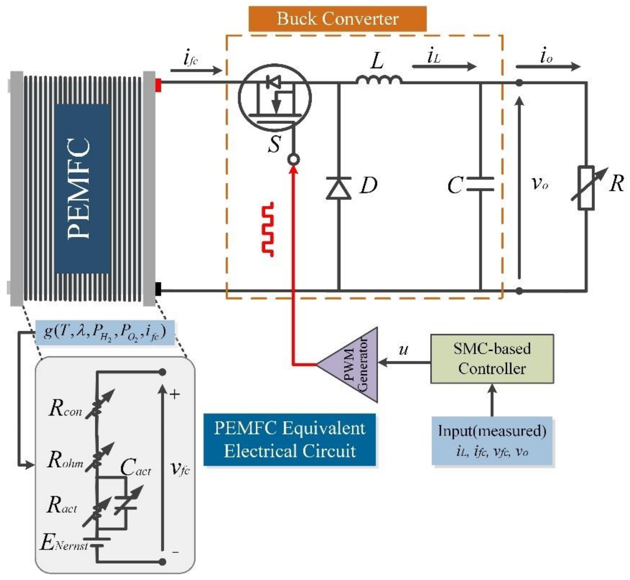
2. PEMFC Power Supply Modeling

The power supply system consists of a PEMFC and DC/DC buck converter. The PEMFC generates electricity, and DC/DC buck converter regulates load current or stabilizes the output voltage, which can be used for battery constant current charging or constant voltage charging in the electric vehicles [41,42]. The model of the power supply system is constructed based on the equivalent circuit methods.

2.1. Model of PEMFC

Equations (1) and (2) involve static and dynamic characteristics of PEMFC, respectively. The variable double-layer capacitor effect is applied to simulate the dynamics of PEMFC [3,4].
v f c = N E N e r n s t V o h m V c o n V C
d V C d t = 1 C a c t i f c V C R a c t
where ENernst is the reversible voltage, and Vohm is the ohmic drop. VC is the voltage of capacitor Cact, and Vact is the activation drop. vfc is PEMFC voltage, and N is the number of cells. ifc is PEMFC current, and Cact is variable capacity. Ract is activation polarization resistance.
The relation between vfc and ifc can be described as [4]:
v f c = g i f c , P H 2 , P O 2 , T
where T is the working temperature of PEMFC. λ is the average water content in the membrane, which is based on the membrane humidity [3]. P H 2 and P O 2 are the pressure of hydrogen and oxygen, respectively.

2.2. Model of PEMFC Power Supply System

The circuit diagram of the power supply is shown in Figure 1. It is composed of an inductor L, a capacitor C, an output load R, a MOSFET switch S, and a diode D. In addition, vfc, io, and vo represent stack voltage, load current, and load voltage, respectively.
The average model of PEMFC-fed DC/DC buck converter is described as:
d i L d t = 1 L u v f c v o d v o d t = 1 C i L v o R
where iL is inductive current and vo is the output load voltage. u represents the switch status, ranging from 0 (switch is OFF) to 1 (switch is ON).
The following assumptions are introduced to simplify the plant for the control-orientation.
Assumption 1.
The inductance is large enough to provide continuous inductive current to ensure the system is operating under a continuous conduction mode (CCM).
Assumption 2.
When the MOSFET S is on, the resistance of it is zero while the diode D has no drop voltage.
Assumption 3.
All the passive elements are ideal.
Assumption 4.
The working pressure of PEMFC is presented at P H 2 = 20,265 Pa, P A i r = 101,325 Pa. In addition, T = 333.15 K, a high efficiency operation temperature is used.
In practice, there may be parametric uncertainties and disturbance injections existing in the average model. A practical model is considered as [39]:
d i L d t = 1 L 0 + Δ L u g u i L v o d v o d t = 1 C 0 + Δ C i L v o R 0 + Δ R
where L0, C0, and R0 are the nominal values of L, C, and R, respectively. ΔL, ΔC, and ΔR are variations of L, C, and R, respectively.
Assumption 5.
The variations of L, C, and R are not measurable and unknown. ΔL, ΔC, and ΔR are bounded by positive constants Lm, Cm, and Rm, respectively. That is:
Δ L L m , Δ C C m , Δ R R m
The parameters of DC/DC buck converter and PEMFC system are listed in Table 1.

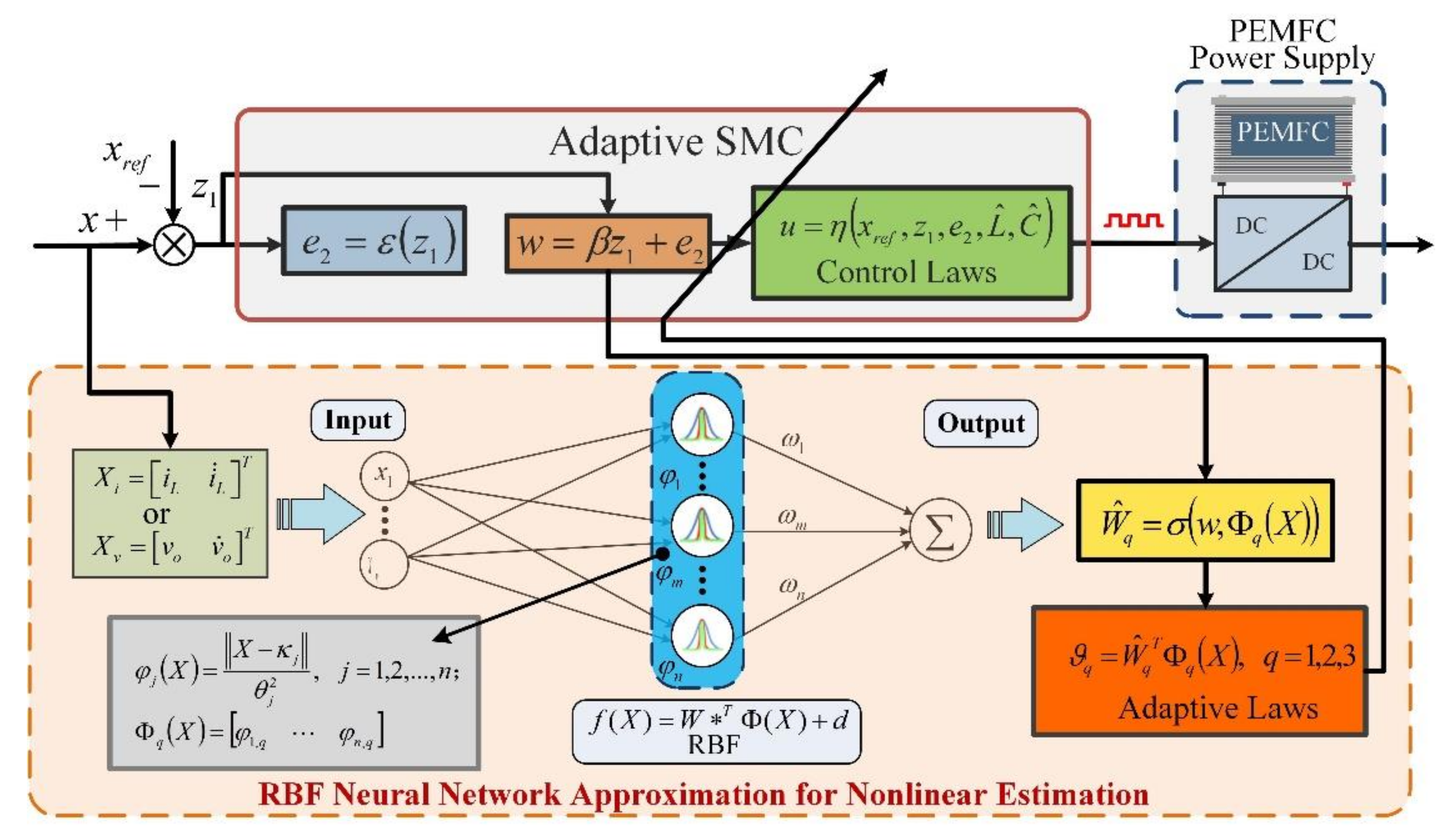
3. Adaptive Control of PEMFC Power Supply

To handle the nonlinearity and uncertainties of PEMFC power supply, an adaptive control based on backstepping SMC and RBFNN estimation is proposed. A SMC controller is firstly designed in this section. An adaptive backstepping SMC is then introduced. Finally, the RBFNN estimator for parametric uncertainties and external disturbance is developed. The proposed controllers meet the demands of the Lyapunov stability theory.

3.1. Model of PEMFC

The control law of SMC is selected in the form of:
u = 1 2 1 s i g n s
where s = i L i L , r e f .
Then, the derivation of s can be obtained by:
s ˙ = 1 L v o + 1 2 1 s i g n s v f c L
where, in the case of s > 0, s i g n s = 1 , s ˙ = 1 L v o 0 ; when s < 0, s i g n s = 1 , s ˙ = v o v f c L 0 , since the output load voltage of the buck converters is smaller than the input voltage. Therefore, the inductor current control is manipulated by the control law represented by Equation (7) satisfying the Lyapunov stability condition ( V ˙ 0 ). Moreover, the output voltage regulation can be calculated by the indirect current controller according to the equations in [43].

3.2. Adaptive SMC Design

In order to address the nonlinearity of PEMFC, the control plant backs up to subsystems z1 and z2, which is combing with SMC to formulate backstepping SMC.
Assumption 6.
The desired value iL,ref and vo,ref are bounded and have n-order derivative. Meanwhile, I L , r e f = i L , r e f i ˙ L , r e f i L , r e f n T and V o , r e f = v o , r e f v ˙ o , r e f v o , r e f n T are bounded.
Remark 1.
If there is an i under a certain parameter, it represents the parameter used in current regulating, and the same as v, i.e., ci is the parameter c used in current regulating and p is the parameter pv used in voltage regulating.
Lemma 1.
If f(x) is a uniformly continuous function and lim t o t f x d x exists, then f(x) converges to zero asymptotically.
The tracking errors z1 are defined as below, where z1,i and z1,v denote current error and voltage error, respectively:
z 1 , i = i L i L , r e f
z 1 , v = v o v o , r e f
To ensure the stability, define the first Lyapunov function V1:
V 1 , i = 1 2 z 1 , i 2
V 1 , v = 1 2 z 1 , v 2
The virtual control values p is represented by:
p i = α i z 1 , i
p v = α v z 1 , v
where αi and αv are positive constants. Via the virtual control values, the second backstepping variables z2 can be obtained by:
z 2 , i = i ˙ L i ˙ L , r e f + p i
z 2 , v = v ˙ o v ˙ o , r e f + p v
The derivative of V1 is expressed as:
V ˙ 1 , i = α i z 1 , i 2 + z 1 , i z 2 , i
V ˙ 1 , v = α v z 1 , v 2 + z 1 , v z 2 , v
Then, the sliding manifolds s are selected as:
s i = β i z 1 , i + z 2 , i
s v = β v z 1 , v + z 2 , v
where β i , β v are positive constants.
To guarantee the stability and to maintain iL and vo on the sliding manifolds, the second Lyapunov function V 2 are defined as:
V 2 , i = V 1 , i + 1 2 s i 2
V 2 , v = V 1 , v + 1 2 s v 2
The control law u is formulated by:
u ˙ i = L 0 v f c β i α i z 1 , i + z 2 , i 1 L 0 C 0 + 1 L 0 C 0 R 0 + u i v f c α i α i L 0 α i i ˙ L , r e f i ¨ L , r e f + m i s i + n i s i g n s i
u v = L 0 C 0 g v f c β v α v z 1 , v + z 2 , v 1 L 0 C 0 1 R 0 C 0 2 + 1 R 0 2 C 0 2 + α v i L C 0 1 R 0 C 0 α v v ˙ o , r e f v ¨ o , r e f + m v s v + n i s i g n s v
where m and n are positive constants.
The derivative of V 2 can be obtained by:
V ˙ 2 , i = α i z 1 , i 2 + z 1 , i z 2 , i m i s i 2 m i n i s i + M i = Z i T α i + m i β i 2 1 2 + m i β i 1 2 + m i β i m i Z i m i n i s i + M i = Z i T Λ Z i m i n i s i + M i
Similarly, V ˙ 2 , v = Z v T Ρ Z V m v n v s v + M v ,
where Ρ = α v + m v β v 2 1 2 + m v β v 1 2 + m v β v m v , Z i = z 1 , i z 2 , i T , Z v = z 1 , v z 2 , v T , α i + m i β i 2 > 0 , α v + m v β v 2 > 0 , M i and M v can be regarded as disturbance caused by ΔL, ΔC, and ΔR.
To make Λ and Ρ positive define matrix, α, m and β, are satisfying:
α m 1 4 + m β > 0
According to Assumption 5, ΔL, ΔC, and ΔR are limited by Lm, Cm, and Rm, respectively. Thus, the maximum values of Mi and Mv are bounded by M i and M v .
Then:
V ˙ 2 , i = Z i T Λ Z i m i n i s i + M i m i n i s i + M i
V ˙ 2 , v = Z v T Ρ Z V m v n v s v + M v m v n v s v + M v
m and n are limited by:
V ˙ 2 m n s + M 0
By integrating Equation (29), yields:
0 m n s M d x 0 V ˙ 2 d x = V 2 0 V 2 <
where l i m x 0 t m n s M ¯ d x is bounded, according to Lemma 1, m n s M converges to zero when t → ∞. In other words, it converges to zero asymptotically. Therefore, the system is asymptotically stable.
Furthermore, the adaptive laws are proposed to estimate parametric variations. L ^ , C ^ , and R ^ are defined as the estimations of L, C, and R, respectively.
Then, the model denoted by Equation (5) can be estimated by:
i ˙ L = ξ 1 T ϑ ^ v ˙ o = ξ 2 T ϑ ^
where ξ 1 = v f c u v o 0 0 , ξ 2 = 0 i L v o T , ϑ ^ = 1 L ^ 1 C ^ 1 R ^ C ^ .
The second backstepping variables e 2 is defined as:
e 2 , i = z 2 , i ξ 1 T ϑ ˜
e 2 , v = z 2 , v ξ 2 T ϑ ˜
where ϑ ˜ = ϑ ϑ ^ .
The sliding manifold w is selected as:
w i = γ i z 1 , i + e 2 , i
w v = γ v z 1 , v + e 2 , v
where γ i and γ v are positive constants.
Define the second Lyapunov function A 2 :
A 2 i = V 1 i + 1 2 e i 2
A 2 v = V 1 v + 1 2 e v 2
To estimate ϑ ^ , define the third Lyapunov function A3:
A 3 , i = A 2 , i + 1 2 ϑ ˜ T Ψ i 1 ϑ ˜
A 3 , v = A 2 , v + 1 2 ϑ ˜ T Ψ v 1 ϑ ˜
where Ψi and Ψv are positive definite matrix.
To eliminate the estimation error ϑ ˜ existing in Equations (38) and (39), the adaptive laws ϑ ˙ are formulated by:
ϑ ^ ˙ i = Ψ i ς 1 , i + w i γ i ξ 1 + α i ξ 1 ϑ ^ 1 ξ 2
ϑ ^ ˙ v = Ψ v ς 1 , v + w v γ v ξ 2 + α v ξ 2 ϑ ^ 3 ξ 2 + ϑ ^ 2 ξ 1
Then, the control law is calculated by:
u ˙ i = 1 v f c ϑ ^ 1 γ i α i z 1 , i + e 2 , i + u i g ˙ u i i L ϑ ^ 1 ϑ ˙ 1 ξ 2 T ϑ ^ 1 + α i ξ 1 T ϑ ^ + ξ 1 T ϑ ^ ˙ α i i ˙ L , r e f i ¨ L , r e f + a i w i + b i s i g n w i
u v = 1 v f c ϑ ^ 1 ϑ ^ 2 γ v α v z 1 , v + e 2 , v v o ϑ ^ 2 ϑ ^ 1 ϑ ^ 3 ξ 2 T ϑ ^ + α v ξ 2 T ϑ ^ + ξ 2 T ϑ ^ ˙ α v v ˙ o , r e f v ¨ o , r e f + a v w v + b v s i g n w v
where a and b are positive constants.
Substitute Equations (40)–(43) into derivative of Equations (38) and (39), A ˙ 3 can be obtained by:
A ˙ 3 , i = α i z 1 , i 2 + z 1 , i e 2 , i a i w i 2 a i b i w i = Z i T α i + a i γ i 2 1 2 + a i γ i 1 2 + a i γ i a i Z i a i b i w i z 1 , i ξ 1 T ϑ ˜ = Z i T Τ Z i a i b i w i z 1 , i ξ 1 T ϑ ˜
Similarly,
A ˙ 3 , v = Z v T Y Z v a v b v w v z 1 , v ξ 2 T ϑ ˜
where Y = α i + a v γ v 2 1 2 + a v γ v 1 2 + a v γ v a v .
If α, a, and γ are satisfying α a 1 4 + a γ > 0 , the matrix T and Y are positive define matrix. Then,
A ˙ 3 , i a i b i w i z 1 , i ξ 1 T ϑ ˜
A ˙ 3 , v a v b v w v z 1 , v ξ 2 T ϑ ˜
Moreover,
z 1 , i ξ 1 T ϑ ˜ = i L i L , r e f v f c v o 1 L 0 + Δ L 1 L ^
z 1 , v ξ 2 T ϑ ˜ = v o v o , r e f i L 1 C 0 + Δ C 1 C ^ v o 1 R 0 + Δ R C 0 + Δ C 1 R ^ C ^
According to Assumption 5, z 1 , i ξ 1 T ϑ ˜ and z 1 , v ξ 2 T ϑ ˜ are bounded, and the upper bound are defined as:
z 1 , i ξ 1 T ϑ ˜ N i
z 1 , v ξ 2 T ϑ ˜ N v
If a and b are satisfied as:
N i a i b i w i 0
N v a v b v w v 0
Then:
A ˙ 3 , i N i a i b i w i 0
A ˙ 3 , v N v a v b v w v 0
Yielding,
0 a v w N d x 0 A ˙ 3 d x <
According to Lemma 1, a b w N converges to zero. The system is stable asymptotically.

3.3. RBFNN Estimation

The nonlinear estimator based on the RBFNN is developed to deal with the complicated perturbations. The control schematic diagram is shown in Figure 2, and x represents iL or vo when inductor current or load voltage is regulated.
Lemma 2.
RBFNN can model the unknown and continuous function f(X): Rl → R with an ideal weight vector ω* ϵ Rn, the basic function vector Φ X = φ 1 X φ n X T . f(X) is described by RBFNN as:
f X = W * T Φ X + d  
where d is an approximation error bounded by d d . W * = ω 1 * ω n * T , ω* is denoted as the weigh to minimize the norm of approximation error for all X Ω R l , expressed by:
ω j * = arg m i n ω ^ Ω s u p X Ω f X ω ^ T φ X , j = 1 , 2 , n  
where W ^ R n is the estimation of RBF optimal weight vector W * . The Gaussian function is chosen as the basic function,
φ j X = exp || X κ j || θ j 2 , j = 1 , 2 , . . , n  
where κj is the position of the j-th neuron, θj is the center width of the j-th neuron.
The approximation of f(X) is given by:
f ^ X = W ^ T Φ X
and for the system f ^ X = ϑ ^ X , ω ^ = 1 L ^ 1 C ^ 1 R ^ C ^ T .
Determine the inputs of RBFNN by:
X i = i L i ˙ L T
X v = v o v ˙ o T
The estimations are formulated by:
ϑ ^ q = W ^ q T Φ q X
where W ^ q = ω 1 , q ω n , q T and Φ q X = φ 1 , q X φ n , q X T , q = 1, 2, 3.
Define Lyapunov function B3:
B 3 = A 2 + 1 2 χ 1 W ˜ a T W a + 1 2 χ 2 W ˜ b T W b + 1 2 χ 3 W ˜ c T W c
where χ r (r = 1, 2, 3) are positive constants, W ˜ = W * W ^ .
The weight vector adaptive laws W ^ ˙ and control laws u are selected as:
W ^ ˙ a , i = w i χ 1 , i Φ a , i u i v ˙ f c + u ˙ i v f c ϑ ^ 1 i L + v o ϑ ^ 3 + α i ( u i v ˙ f c ) α i v o
W ^ ˙ b , i = w i χ 2 , i Φ b , i ϑ ^ 1 i L
W ^ ˙ c , i = w i χ 3 , i Φ c , i v o ϑ ^ 1
u ˙ i = 1 v f c ϑ ^ 1 γ i α i z 1 , i + e 2 , i + u i v ˙ f c ϑ ^ 1 ϑ ^ 1 ϑ ^ 2 i L + ϑ ^ 1 ϑ ^ 3 v o + ϑ ^ 1 α i v ˙ f c u i v o α i i ˙ L , r e f i ¨ L , r e f + a i w i + b i s i g n w i
W ^ ˙ a , v = w v χ 1 , v Φ a , v v f c u v v o ϑ ^ 2
W ^ ˙ b , v = w v χ 2 , v Φ b , v v f c u v v o ϑ ^ 1 i L ϑ ^ 3 + α v i L
W ^ ˙ c , v = w v χ 3 , v Φ c , v i L ϑ ^ 2 α v v o
u v = 1 v f c ϑ ^ 2 ϑ ^ 1 γ v α v z 1 , v + e 2 , v v o ϑ ^ 2 ϑ ^ 1 + v o ϑ ^ 3 2 i L ϑ ^ 2 ϑ ^ 3 + α v i L ϑ ^ 2 α v v o ϑ ^ 3 α v v ˙ o , r e f v ¨ o , r e f + a v w v + b v s i g n w v
Similar to Equations (44)–(56), the stable solutions can be found. Compared to Equations (40) and (41), the uncertainties and disturbances are estimated via nonlinear Gaussian function Φ(X). The approach can improve the accuracy of the estimation even complicated perturbations occurring.

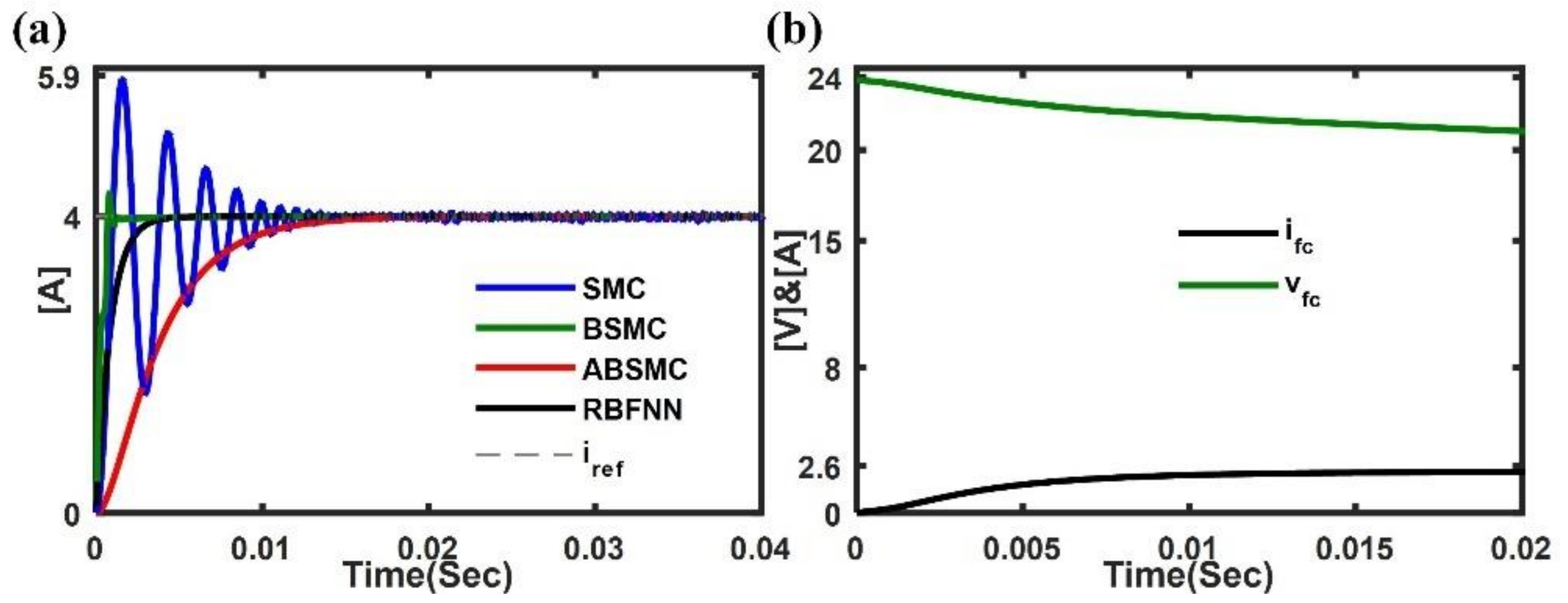
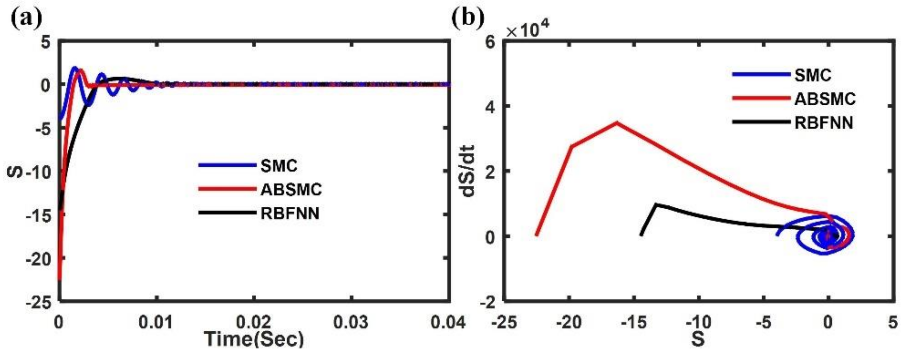
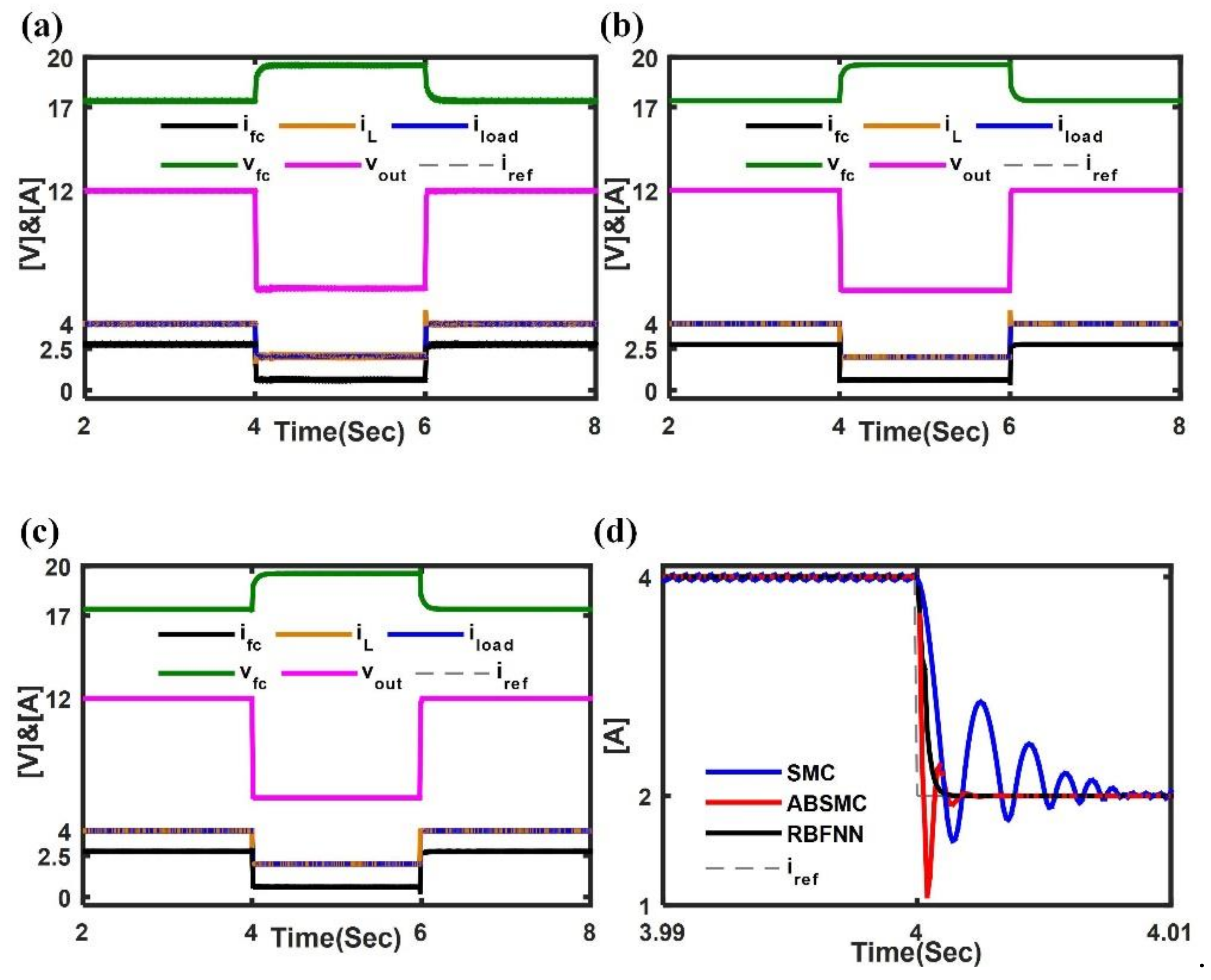
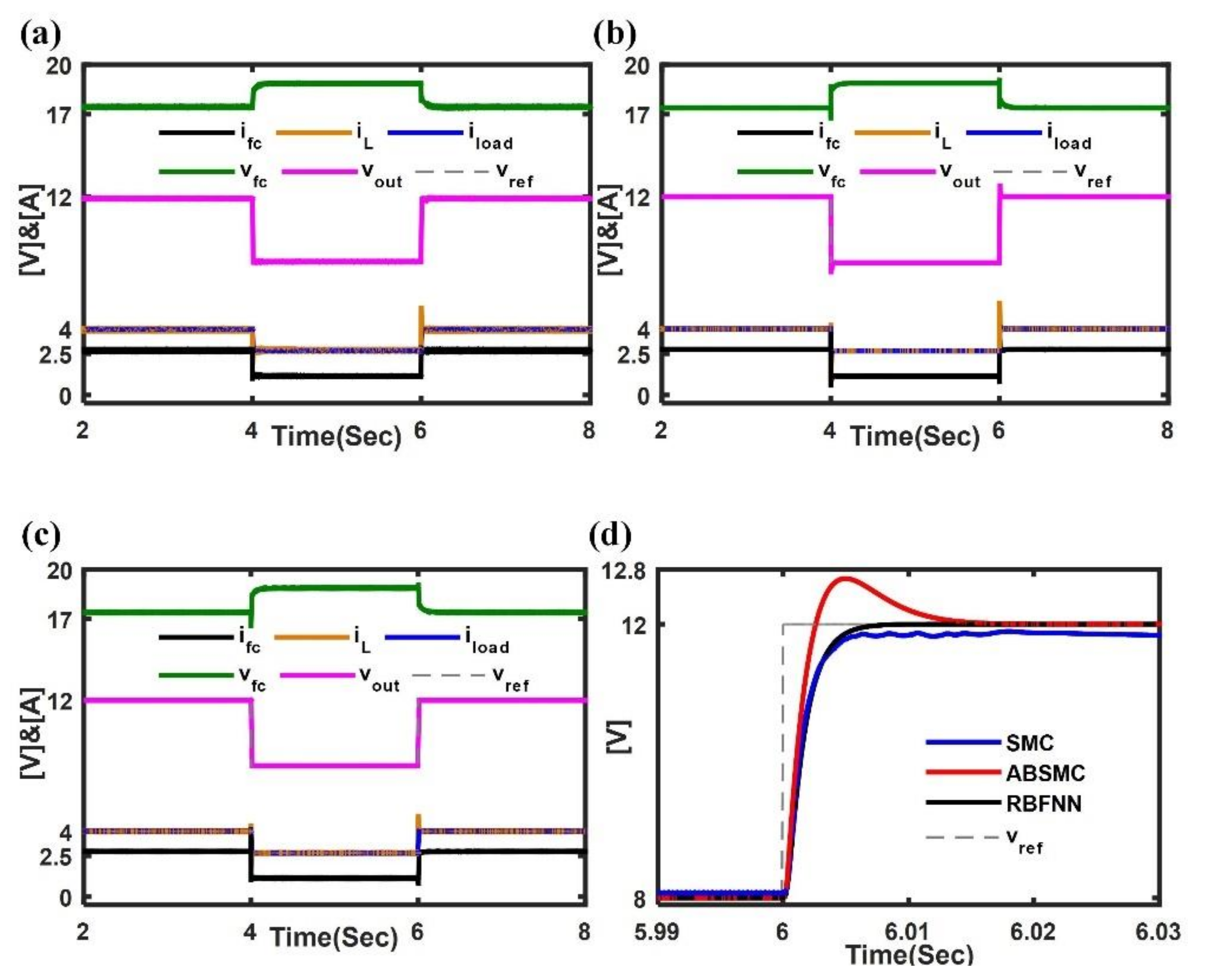
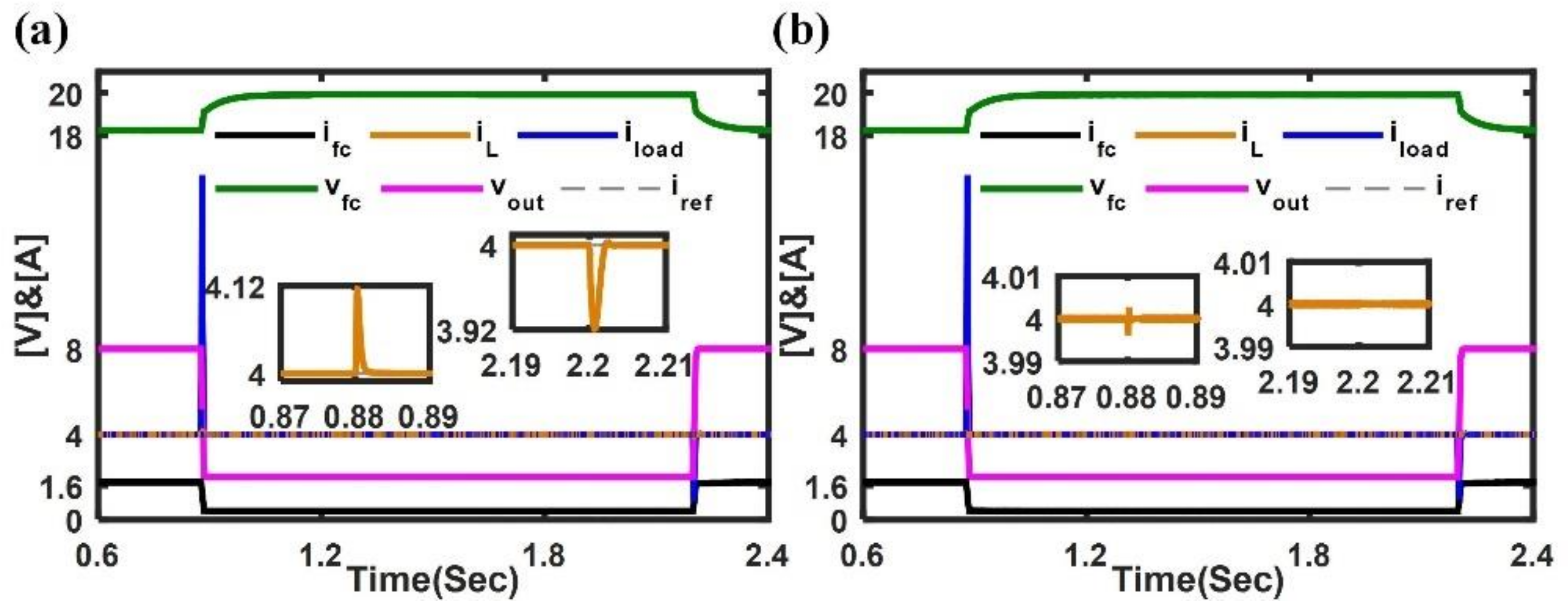
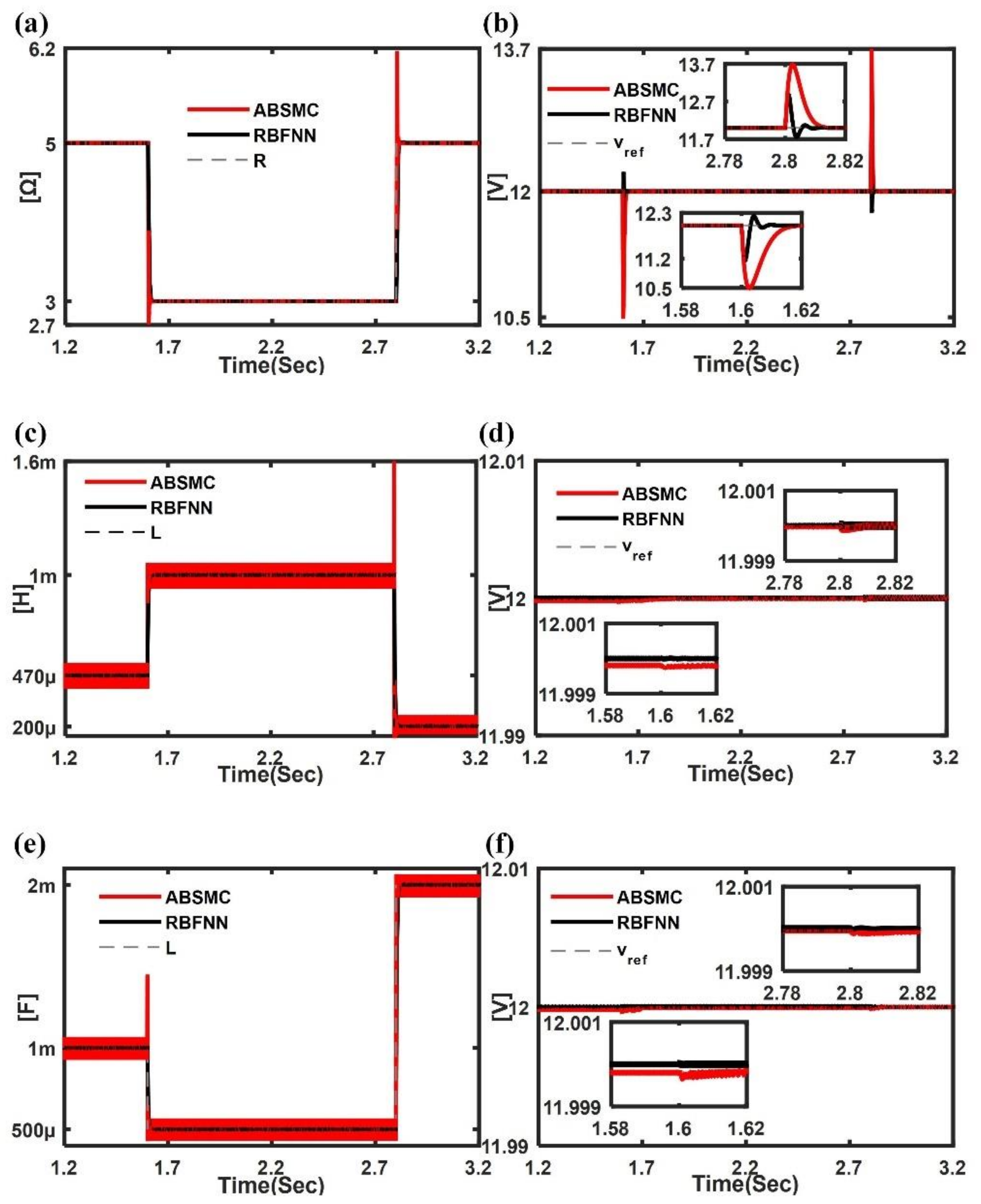
4. Simulation and Discussion

Numerical simulation and experimental tests are carried out on PEMFC power supply for the proposed controllers and observers under the given test conditions listed in Table 2.
H-100 PEMFC with 100 W rate power is selected to feed DC/DC buck converter to configure the power supply, and L0 = 470 μH and C0 = 1000 μF are the nominal values of the converter. The test conditions are mainly used for checking the transient response and the tracking performance as well as the robustness against uncertainties and disturbances.
The results of different control techniques in Condition 1 are shown in Figure 3. The simulation analysis results show that the response time of the output current controlled by backstepping SMC (BSMC) is the fastest, but the overshoot of the output current is obvious. The response time of the output current controlled by SMC is 0.014 s, which is similar to the control result of adaptive backstepping SMC (ABSMC). Compared with RBF control performance, it is 0.011 s slower. In addition, from the response stage, the current controlled by the SMC has an obvious oscillation phenomenon. Regardless of whether it is considered from the protection of the life of the fuel cell or the utilization of electric energy on the output side, this phenomenon will have an adverse effect. In contrast, the output current response stage of ABSMC and RBF control is relatively smooth. At the same time, the RBF adaptive controller has the advantages of faster response speed, no overshoot, no overshoot phenomenon in the output voltage, and the fuel cell current/voltage overshoot range is within an acceptable range.
Moreover, by exploring the sliding manifolds and the associate trajectories in the phase plane displayed in Figure 4a,b, the typical reaching behaviors of the designed controllers were manifested, and the RBFNN presented a high convergence precision.
In Condition 2, the tracking setpoints were abruptly changed at the constant load condition. The load was rapidly changing from 4 A to 2 A at 4 s and 2 A to 4 A at 6 s. The current controlled by the SMC and ABSMC has an obvious oscillation phenomenon. The controller with RBFNN indicates the best performance (see Figure 5), where the settling time in current tracking control is 0.002 s and 0.005 s in output voltage tracking control. In Condition 3 and 4, the tracking setpoints were abruptly changed at the constant load condition, the controller with RBFNN indicates the best performance (see Figure 6 and Figure 7), where the settling time in current tracking control is 0.002 s and 0.006 s in output voltage tracking control, without overshoot and undershoot. Additionally, small chattering problems on PEMFC voltage and current were observed when SMC acted, and small undershoots on PEMFC current were caused by tracking step-down reference voltage governed by adaptive controllers. Due to the load demand changing, the PEMFC operation point may vary to adapt for the converter desired output voltage or current.
Figure 7a,b exhibited the simulation results regulated by the adaptive backstepping SMC and RBFNN, respectively. In the adaptive backstepping SMC, the settling time in current tracking control is 0.0015 s. The maximum overshoot is about 3% (0.12 A), and the maximum undershoot is about 2% (0.08 A). In addition, depending on RBFNN estimation, the overshoots and undershoots are almost eliminated.
The external disturbance estimation was presented in Figure 8a where the load was rapidly changing from 5 Ω to 3 Ω at 1.6 s and 3 Ω to 5 Ω at 2.8 s as the Condition 5 depicted. The traditional adaptive law and RBFNN achieved resistance estimation; however, the traditional scheme led in large overshoot or undershoot of resistance that might postpone output reach to setpoint as illustrated in Figure 8b. In the adaptive backstepping SMC, the maximum overshoot is about 14.2% (1.7 V), and the maximum undershoot is about 12.5% (1.5 V). In the RBFNN, the maximum overshoot is about 5.8% (0.7 V), and the maximum undershoot is about 1.7% (0.2 V). Furthermore, to investigate the structural parameters variation caused by perturbations on the inductor and capacitor of the power supply, the traditional adaptive law and RBFNN are also compared. The simulation profiles of L and C were shown in Figure 8c–e, the estimations based on RBFNN matched the real profiles of both L and C well. Additionally, the output voltage tracking control in the cases of L or C variations via the proposed methods demonstrated good performance. The results of comparison tests under Conditions 1–5 are presented in Table 3.

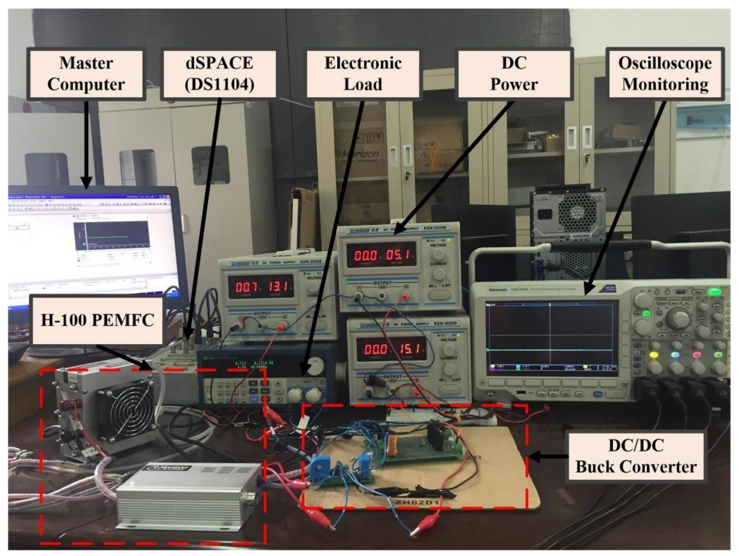
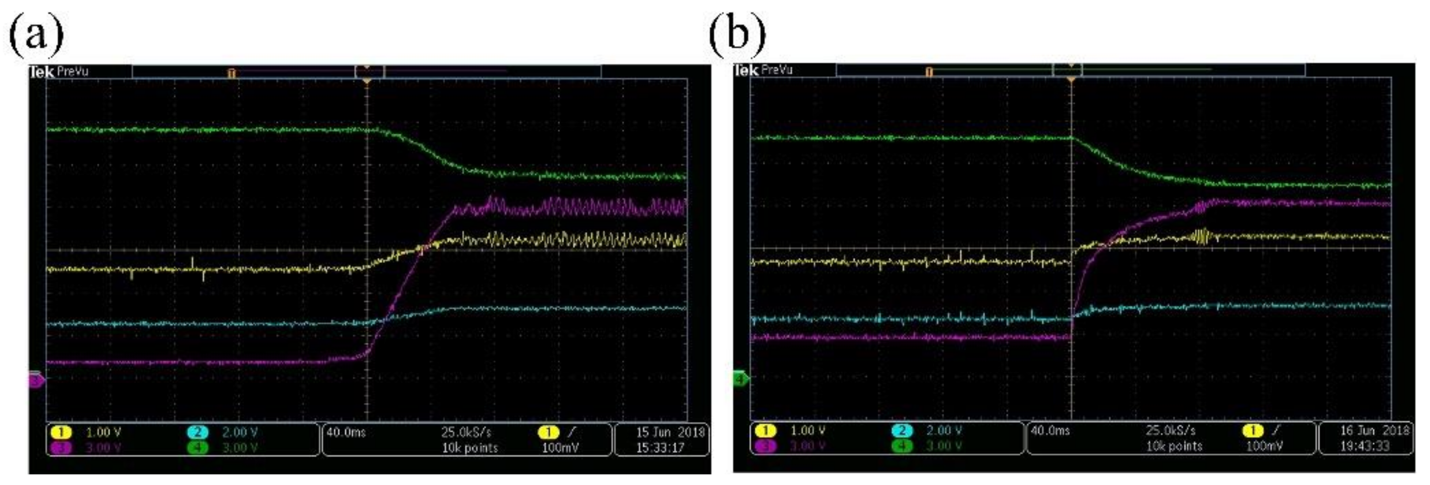
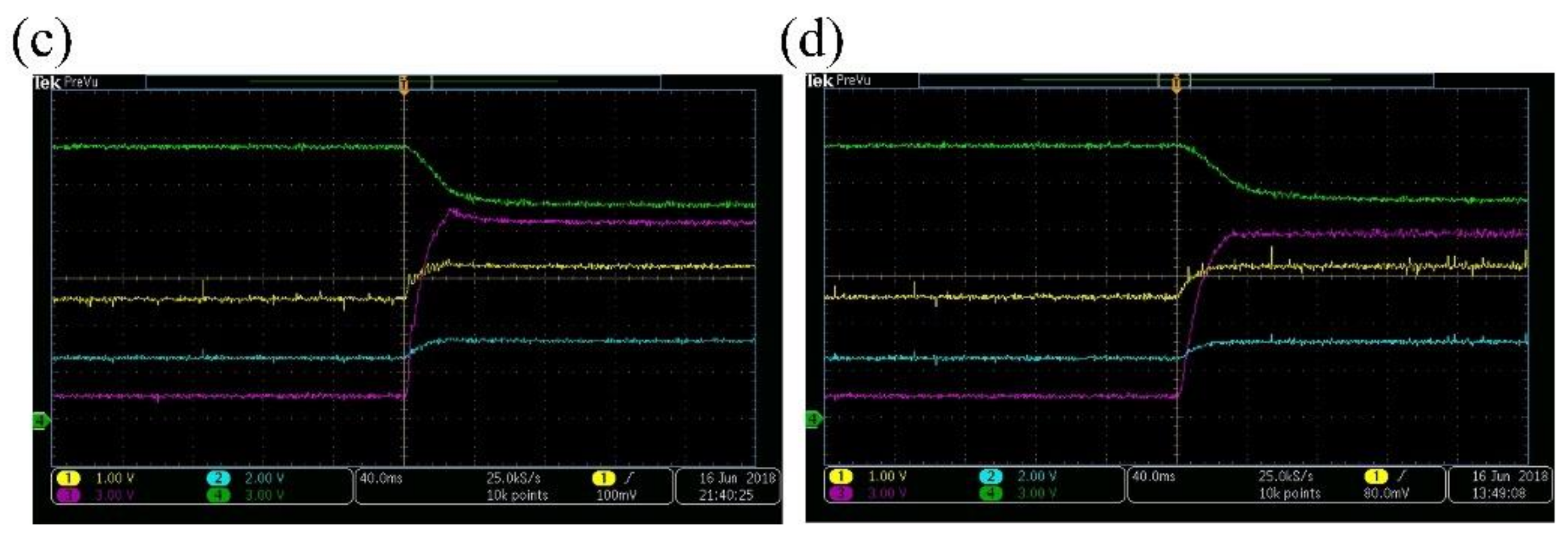
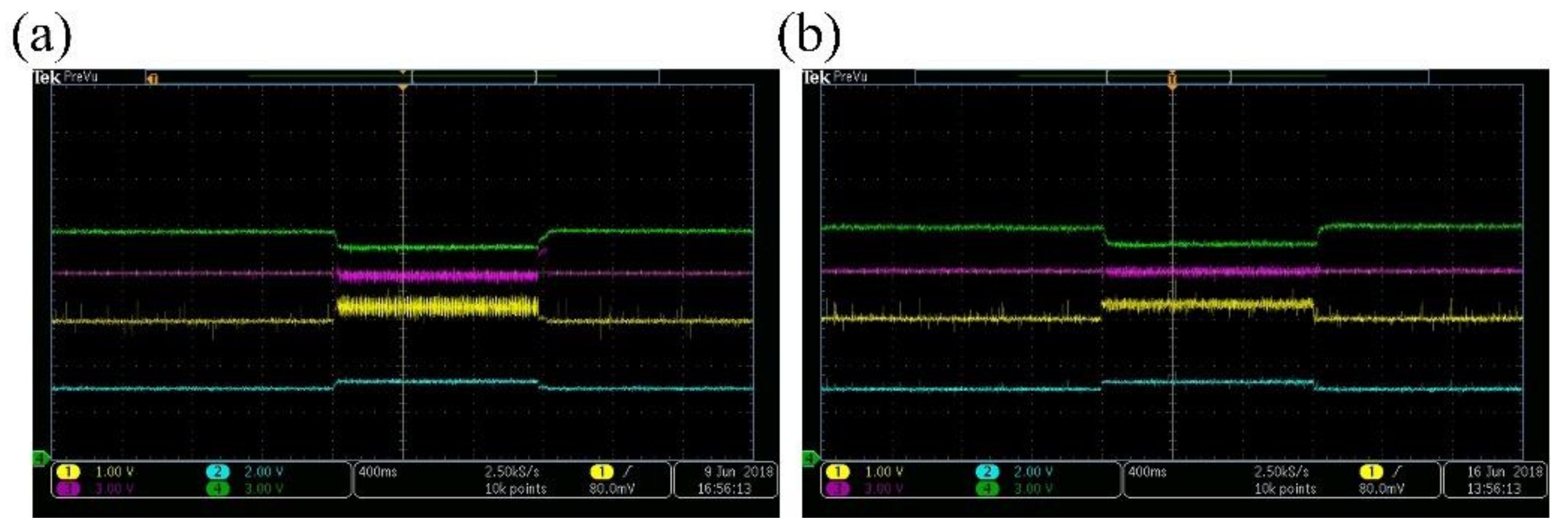
5. Experimental Validation

An experimental PEMFC power supply prototype is set up to validate the efficiency of the proposed control approaches. Besides the H-100 PEMFC and DC/DC buck converter, a dSPACE DS1104 controller board, M9710 DC electronic load, KXN-3020D DC power source, and Tektronix MDO3054 digital phosphor oscilloscope comprise the test platform, as shown in Figure 9. The currents were measured by HCS-LSP hall sensor by the conversion relation between sensor output voltage Uo and real measured current Ir, i.e., Ir = (Uo−2.5) × 5. Figure 10 and Figure 11 illustrated the experimental results where Channel 1 to Channel 4 represented inductor current, load current, load voltage, and PEMFC voltage, respectively.
In Figure 10a,b, the transient responses (tested in Condition 1) of inductor current tracking control were given, where the traditional SMC presented a chattering phenomenon and the maximum amplitude was about 4.5 A, and the results of traditional adaptive backstepping SMC exhibited local chattering. RBFNN-based current and voltage control results were shown in Figure 10c,d, and their transient performances exhibiting fast settling time and no overshoot were better than the traditional methods.
Finally, the load resistance variation experiments (tested in Condition 5) were conducted to examine the disturbance rejection ability. Figure 11 indicated that the adaptive output voltage controls tracked setpoint, and RBFNN reduced up to 7.5% overshoot and smoothed PEMFC voltage and inductor current while disturbance was changing.

6. Conclusions

This paper introduces the RBFNN estimation-based adaptive SMC technique for PEMFC integrated with DC/DC buck converter power supply system. The model of the presented PEMFC power supply has been introduced, where the state and input disturbance of the plant are highly coupled. A Gaussian-based RBF neural network adaptive law with a backstepping SMC scheme is developed according to the defined Lyapunov functions to handle the parametric uncertainties and disturbance injections, such as buck converter parameter-varying and PEMFC operation point changing. The comparative study is carried out to regulate PEMFC power supply current/voltage on H-100 PEMFC supplied DC/DC buck converter with rapid control prototyping among traditional SMC, adaptive backstepping SMC, and RBF neural network. The simulation analysis and experimental results indicate that the proposed method can track the desired current/voltage with enhanced robustness; for instance, compared with the traditional adaptive law, even with the abrupt change of load occurring, about 3% overshoot was reduced in the case of inductor current control simulation, and up to 7.5% overshoot was reduced in output voltage regulation experimental test. The proposed control system can be applied in many industrial applications, such as automotive air conditioning and charging energy storage devices, such as batteries and super-capacitors, with the desired charging current or terminal voltage.

Author Contributions

Conceptualization, X.X. and H.H.; methodology, X.X., J.L. and H.H.; software, J.C.; validation, H.H., Y.C. and J.C.; formal analysis, X.X.; investigation, J.L. and Y.C.; resources, H.H.; data curation, X.X. and H.H.; writing—original draft preparation, X.X. and J.L.; writing—review and editing, X.X., J.L., Y.C. and H.H.; visualization, X.X.; supervision, J.L. and H.H.; project administration, H.H. and J.C.; funding acquisition, J.L. and H.H. All authors have read and agreed to the published version of the manuscript.

Funding

This research received no external funding.

Institutional Review Board Statement

This study did not involve humans.

Informed Consent Statement

This study did not involve humans.

Data Availability Statement

This study did not report any data.

Conflicts of Interest

The authors declare no conflict of interest.

Nomenclature

vVoltage (V)
iCurrent (A)
λAverage water content
PPressure (Pa)
TTemperature (K)
CCapacity (F)
RResistance (Ω)
LInductance (H)
uControl law
pVirtual control values
ALyapunov function
BLyapunov function
WWeight
Subscripts
0Nominal value
actActivation
AirAir
CCapacitor
conConcentration
ohmOhmic
fcFuel cell
H2Hydrogen
iUsed in current regulating
O2Oxygen
refReference
vUsed in voltage regulating

References

  1. Chatrattanawet, N.; Hakhen, T.; Kheawhom, S.; Arpornwichanop, A. Control structure design and robust model predictive control for controlling a proton exchange membrane fuel cell. J. Clean. Prod. 2017, 148, 934–947. [Google Scholar] [CrossRef]
  2. Harrag, A.; Messalti, S. How fuzzy logic can improve PEM fuel cell MPPT performances. Int. J. Hydrog. Energy 2018, 43, 537–550. [Google Scholar] [CrossRef]
  3. Giaouris, D.; Stergiopoulos, F.; Ziogou, C.; Banerjee, S.; Zahawi, B.; Pickert, V.; Voutetakis, S.; Papadopoulou, S. Nonlinear stability analysis and a new design methodology for a PEM fuel cell fed DC–DC boost converter. Int. J. Hydrog. Energy 2012, 37, 18205–18215. [Google Scholar] [CrossRef]
  4. Wang, Y.X.; Yu, D.H.; Chen, S.A.; Kim, Y.B. Robust DC/DC converter control for polymer electrolyte membrane fuel cell application. J. Power Sources 2014, 261, 292–305. [Google Scholar] [CrossRef]
  5. Debenjak, A.; Petrovčič, J.; Boškoski, P.; Musizza, B.; Juričić, Đ. Fuel cell condition monitoring system based on interconnected DC–DC converter and voltage monitor. IEEE Trans. Ind. Electron. 2017, 62, 5293–5305. [Google Scholar] [CrossRef]
  6. Valdez-Resendiz, J.; Rosas-Caro, V.S.J.; Maldonado, M.; Sierra, J.; Barbosa, R. Continuous input-current buck-boost DC-DC converter for PEM fuel cell applications. Int. J. Hydrog. Energy 2017, 42, 30389–30399. [Google Scholar] [CrossRef]
  7. Sun, F.; Xiong, R.; He, H. A systematic state-of-charge estimation framework for multi-cell battery pack in electric vehicles using bias correction technique. Appl. Energy 2016, 162, 1399–1409. [Google Scholar] [CrossRef]
  8. Wang, Y.X.; Ou, K.; Kim, Y.B. Modeling and experimental validation of hybrid proton exchange membrane fuel cell/battery system for power management control. Int. J. Hydrog. Energy 2015, 40, 11713–11721. [Google Scholar] [CrossRef]
  9. Afsharinejad, A.; Asemani, M.H.; Dehghani, M.; Abolpour, R.; Vafamand, N. Optimal gain-scheduling control of proton exchange membrane fuel cell: An LMI approach. IET Renew. Power Gener. 2022, 16, 459–469. [Google Scholar] [CrossRef]
  10. Bayram, M.B.; Sefa, I.; Balci, S. A static exciter with interleaved buck converter for synchronous generators. Int. J. Hydrog. Energy 2017, 42, 17760–17770. [Google Scholar] [CrossRef]
  11. Wang, Y.X.; Ou, K.; Kim, Y.B. Power source protection method for hybrid polymer electrolyte membrane fuel cell/lithium-ion battery system. Renew. Energy 2017, 111, 381–391. [Google Scholar] [CrossRef]
  12. Lian, K.Y.; Liou, J.J.; Huang, C.Y. LMI-based integral fuzzy control of DC-DC converters. IEEE Trans. Fuzzy Syst. 2006, 14, 71–80. [Google Scholar] [CrossRef]
  13. Sumsurooah, S.; Odavic, M.; Bozhko, S.; Boroyevich, D. Robust stability analysis of a DC/DC buck converter under multiple parametric uncertainties. IEEE Trans. Power Electron. 2017, 33, 5426–5441. [Google Scholar] [CrossRef] [Green Version]
  14. Olalla, C.; Leyva, R.; El Aroudi, A.; Queinnec, I. Robust LQR control for PWM converters: An LMI approach. IEEE Trans. Ind. Electron. 2009, 56, 2548–2558. [Google Scholar] [CrossRef]
  15. Geyer, T.; Papafotiou, G.; Morari, M. Hybrid model predictive control of the step-down DC–DC converter. IEEE Trans. Control Syst. Technol. 2008, 16, 1112–1124. [Google Scholar] [CrossRef]
  16. Liu, Z.; Xie, L.; Lu, S.; Bemporad, A. Fast linear parameter varying model predictive control of buck DC–DC converters based on FPGA. IEEE Access 2018, 6, 52434–52446. [Google Scholar] [CrossRef]
  17. Wang, J.; Li, S.; Yang, J.; Wu, B.; Li, Q. Extended state observer-based sliding mode control for PWM-based DC–DC buck power converter systems with mismatched disturbances. IET Control Theory Appl. 2015, 9, 579–586. [Google Scholar] [CrossRef]
  18. Ahmeid, M.; Armstrong, M.; Gadoue, S.; Gadoue, S.; Algreer, M.; Missailidis, P. Real-time parameter estimation of DC–DC converters using a self-tuned Kalman filter. IEEE Trans. Power Electron. 2016, 32, 5666–5674. [Google Scholar] [CrossRef] [Green Version]
  19. Ding, S.; Zheng, W.-X.; Sun, J.; Wang, J. Second-order sliding-mode controller design and its implementation for buck converters. IEEE Trans. Ind. Inform. 2017, 14, 1990–2000. [Google Scholar] [CrossRef]
  20. Ma, R.; Wu, Y.; Breaz, E.; Huangfu, Y.; Briois, P.; Gao, F. High-order sliding mode control of DC–DC converter for PEM fuel cell applications. In Proceedings of the 2018 IEEE Industry Applications Society Annual Meeting (IAS), Portland, OR, USA, 23–27 September 2018; pp. 1–7. [Google Scholar]
  21. Hernández-Méndez, A.; Linares-Flores, J.; Sira-Ramírez, H.; Guerrero-Castellanos, J.F.; Mino-Aguilar, G. A backstepping approach to decentralized active disturbance rejection control of interacting boost converters. IEEE Trans. Ind. Appl. 2017, 53, 4063–4072. [Google Scholar] [CrossRef]
  22. Fehr, H.; Gensior, A. On trajectory planning, backstepping controller design and sliding modes in active front-ends. IEEE Trans. Power Electron. 2016, 31, 6044–6056. [Google Scholar] [CrossRef]
  23. Sker, M.; Zergeroglu, E. Nonlinear control of flyback type DC to DC Converters: An indirect backstepping approach. In Proceedings of the 2011 IEEE International Conference on Control Applications (CCA), Denver, CO, USA, 28–30 September 2011; pp. 65–69. [Google Scholar]
  24. Dahech, K.; Allouche, M.; Damak, T.; Tadeo, F. Backstepping sliding mode control for maximum power point tracking of a photovoltaic system. Electr. Power Syst. Res. 2017, 143, 182–188. [Google Scholar] [CrossRef]
  25. Salimi, M.; Soltani, J.; Markadeh, G.A.; Abjadi, N.R. Indirect output voltage regulation of DC–DC buck/boost converter operating in continuous and discontinuous conduction modes using adaptive backstepping approach. IET Power Electron. 2013, 6, 732–741. [Google Scholar] [CrossRef] [Green Version]
  26. McIntyre, M.L.; Schoen, M.; Latham, J. Simplified adaptive backstepping control of buck DC:DC converter with unknown load. In Proceedings of the 2013 IEEE 14th Workshop on Control and Modeling for Power Electronics (COMPEL), Salt Lake City, UT, USA, 23–26 June 2013; pp. 1–7. [Google Scholar]
  27. Nizami, T.K.; Chakravarty, A.; Mahanta, C. Analysis and experimental investigation into a finite time current observer based adaptive backstepping control of buck converters. J. Frankl. Inst. 2018, 355, 4996–5017. [Google Scholar] [CrossRef]
  28. Zuniga-Ventura, Y.A.; Langarica-Cordoba, D.; Leyva-Ramos, J.; Diaz-Saldierna, L.H.; Ramírez-Rivera, V.M. Adaptive backstepping control for a fuel cell/boost converter system. IEEE J. Emerg. Sel. Top. Power Electron. 2018, 6, 686–695. [Google Scholar] [CrossRef]
  29. Wang, C.; Tian, H. Research on Control Strategy of Interleaved BUCK Circuit Based on BP Neural Network Model. In Proceedings of the 2019 14th IEEE Conference on Industrial Electronics and Applications (ICIEA), Xi’an, China, 19–21 June 2019; pp. 2009–2013. [Google Scholar]
  30. Zhang, L.; Chen, K.; Chi, S.; Lyu, L.; Ma, H.; Wang, K. The Bidirectional DC/DC Converter Operation Mode Control Algorithm Based on RBF Neural Network. In Proceedings of the 2019 IEEE Innovative Smart Grid Technologies—Asia (ISGT Asia), Chengdu, China, 21–24 May 2019; pp. 2138–2143. [Google Scholar]
  31. Jin, H.; Zhao, X. Complementary sliding mode control via elman neural network for permanent magnet linear servo system. IEEE Access 2019, 7, 82183–82193. [Google Scholar] [CrossRef]
  32. Chu, Y.; Hou, S.; Fei, J. Continuous terminal sliding mode control using novel fuzzy neural network for active power filter. Control Eng. Pract. 2021, 109, 104735. [Google Scholar] [CrossRef]
  33. Liu, Y.-C.; Laghrouche, S.; N’Diaye, A.; Cirrincione, M. Hermite neural network-based second-order sliding-mode control of synchronous reluctance motor drive systems. J. Frankl. Inst. 2021, 358, 400–427. [Google Scholar] [CrossRef]
  34. Peng, C.; Bai, Y.; Gong, X.; Gao, Q.; Zhao, C.; Tian, Y. Modeling and robust backstepping sliding mode control with adaptive RBFNN for a novel coaxial eight-rotor UAV. IEEE/CAA J. Autom. Sin. 2015, 2, 56–64. [Google Scholar]
  35. Fu, C.; Hong, W.; Lu, H.; Zhang, L.; Guo, X.; Tian, Y. Adaptive robust backstepping attitude control for a multi-rotor unmanned aerial vehicle with time-varying output constraints. Aerosp. Sci. Technol. 2018, 78, 593–603. [Google Scholar] [CrossRef]
  36. Xu, D.; Liu, J.; Yan, X.-G.; Yan, W. A novel adaptive neural network constrained control for a multi-area interconnected power system with hybrid energy storage. IEEE Trans. Ind. Electron. 2018, 65, 6625–6634. [Google Scholar] [CrossRef]
  37. Wang, Z.; Hu, C.; Zhu, Y.; He, S.; Yang, K.; Zhang, M. Neural network learning adaptive robust control of an industrial linear motor-driven stage with disturbance rejection ability. IEEE Trans. Ind. Inf. 2017, 13, 2172–2183. [Google Scholar] [CrossRef]
  38. Zeng, X.; Li, Z.; Wan, J.; Zhang, J.; Ren, M.; Gao, W.; Li, Z.; Zhang, B. Embedded hardware artificial neural network control for global and real-time imbalance current suppression of parallel connected IGBTs. IEEE Trans. Ind. Electron. 2019, 67, 2186–2196. [Google Scholar] [CrossRef]
  39. Chi, X.; Quan, S.; Chen, J.; Wang, Y.-X.; He, H. Proton exchange membrane fuel cell-powered bidirectional DC motor control based on adaptive sliding-mode technique with neural network estimation. Int. J. Hydrog. Energy 2020, 45, 20282–20292. [Google Scholar] [CrossRef]
  40. Srinivasan, S.; Tiwari, R.; Krishnamoorthy, M.; Lalitha, M.P.; Raj, K.K. Neural network based MPPT control with reconfigured quadratic boost converter for fuel cell application. Int. J. Hydrog. Energy 2021, 46, 6709–6719. [Google Scholar] [CrossRef]
  41. Peng, J.; He, H.; Xiong, R. Rule based energy management strategy for a series–parallel plug-in hybrid electric bus optimized by dynamic programming. Appl. Energy 2017, 185, 1633–1643. [Google Scholar] [CrossRef]
  42. Yan, M.; Li, M.; He, H.; Peng, J.; Sun, C. Rule-based energy management for dual-source electric buses extracted by wavelet transform. J. Clean. Prod. 2018, 189, 116–127. [Google Scholar] [CrossRef]
  43. Utkin, V. Sliding mode control of DC/DC converters. J. Frankl. Inst. 2013, 350, 2146–2165. [Google Scholar] [CrossRef] [Green Version]
Figure 1. Circuit diagram of PEMFC power supply.
Applsci 12 03132 g001
Figure 2. RBFNN estimation control schematic diagram.
Applsci 12 03132 g002
Figure 3. Simulation results in Condition 1: (a) by different control methods; (b) PEMFC current and voltage response when regulated by RBFNN.
Applsci 12 03132 g003
Figure 4. Current control transient response: (a) sliding manifold S; (b) S vs. dS/dt.
Applsci 12 03132 g004
Figure 5. Simulation results in Condition 2: (a) by SMC; (b) by adaptive backstepping SMC; (c) by RBFNN; (d) inductor current controlled by different control methods, enlarged view at 4 s.
Applsci 12 03132 g005
Figure 6. Simulation results in Condition 3: (a) by SMC; (b) by adaptive backstepping SMC; (c) by RBFNN; (d) output voltage controlled by different control methods, enlarged view at 6 s.
Applsci 12 03132 g006
Figure 7. Simulation results in Condition 4: (a) by adaptive backstepping SMC; (b) by RBFNN.
Applsci 12 03132 g007
Figure 8. Simulation results under parametric variations: (a) Condition 5 R estimation (b) Condition 5 voltage response; (c) L estimation; (d) voltage response depending on L profile; (e) C estimation; (f) voltage response depending on C profile.
Applsci 12 03132 g008
Figure 9. Experimental test for the power supply prototype.
Applsci 12 03132 g009
Figure 10. Transient response: (a) current control by SMC; (b) current control by adaptive backstepping SMC; (c) current control by RBFNN; (d) voltage control by RBFNN.
Applsci 12 03132 g010aApplsci 12 03132 g010b
Figure 11. Disturbance change when applying load step: (a) voltage control by adaptive backstepping SMC; (b) voltage control by RBFNN.
Applsci 12 03132 g011
Table 1. The parameters of DC/DC buck converter and PEMFC system.
ParametersValueUnit
PEMFC power (Pfc)100W
Number of cells (N)20-
Thickness of the membrane (lfc)0.0178cm
Area of the membrane (Afc)22.5cm2
Inductor (L0)470mH
Capacitor (C0)1000μF
Constant resistance (R0)2.05 × 10⁻²Ω
Table 2. Parameters of the test conditions.
Test ConditionsParameters with Time
SetpointsLoad Resistor
Condition 1: current transient responseiL,ref = 4 AR = 3 Ω
Condition 2: step response for different currentiL,ref = 2 A @ [4,6] s; iL,ref = 4 A at other timeR = 3 Ω
Condition 3: step response for different voltagevo,ref = 8 V @ [4,6] s; vo,ref = 12 V at other timeR = 3 Ω
Condition 4: disturbance injection in current controliL,ref = 4 AR = 0.5 Ω @ [0.88, 2.2] s; R = 2 Ω at other time
Condition 5: disturbance injection in voltage controlvo,ref = 12 VR = 3 Ω @ [1.6, 2.8] s; R = 5 Ω at other time
Table 3. Control comparison results under Conditions 1–5.
ConditionsMethodsSettling Time (s)RSME
CurrentVoltageCurrentVoltage
Condition 1ABSMC0.014/0.6317/
RBFNN0.003/0.2836/
Condition 2ABSMC0.003/0.0782/
RBFNN0.002/0.0232/
Condition 3ABSMC/0.012/0.1279
RBFNN/0.006/0.1216
Condition 4ABSMC0.015//0.0284
RBFNN0.001//0.0284
Condition 5ABSMC/0.0100.2018/
RBFNN/0.0040.1794/
Publisher’s Note: MDPI stays neutral with regard to jurisdictional claims in published maps and institutional affiliations.

