
Efficient Fixed-Switching Modulated Finite Control Set-Model Predictive Control Based on Artificial Neural Networks


Abstract
:1. Introduction
2. Conventional FCS-MPC for the 3-Phase 2L-VSI Based on SVPWM
| Algorithm 1: Pseudocode of the conventional MPC with the studied 2L-VSI. |
 |
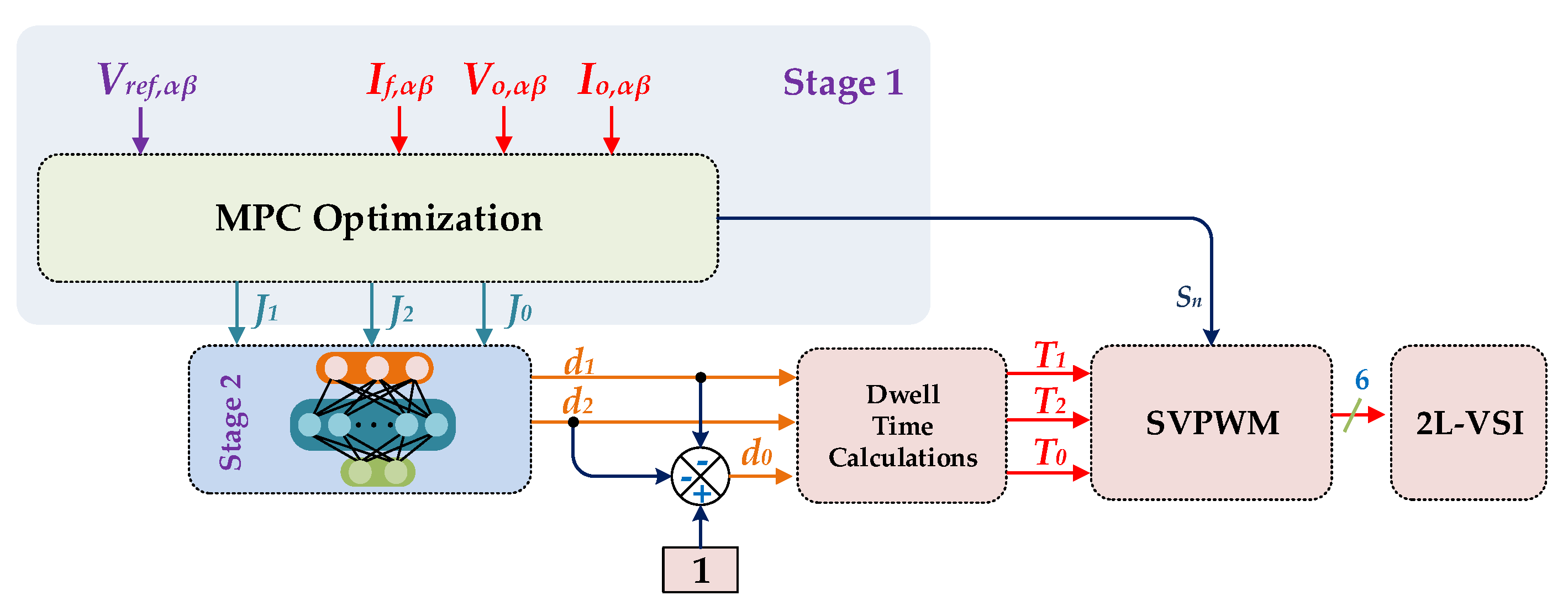
3. Proposed MPC Based-ANN for the 2L-VSI
3.1. Motivation of Using ANN in the Proposed System
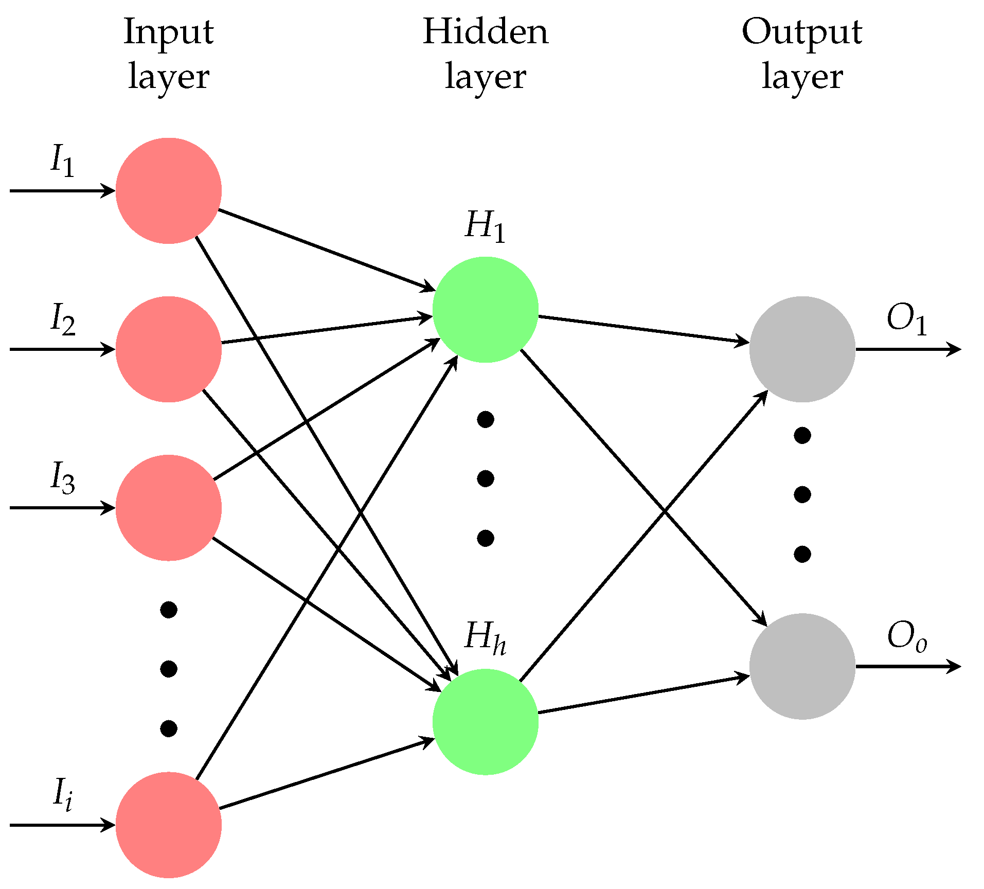
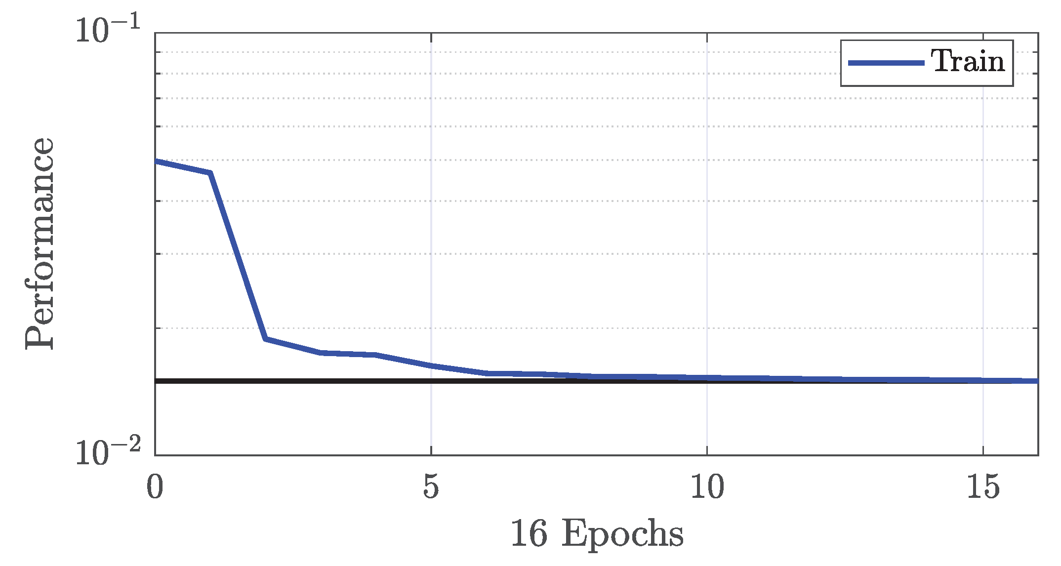
3.2. Description of the Implemented ANN Network
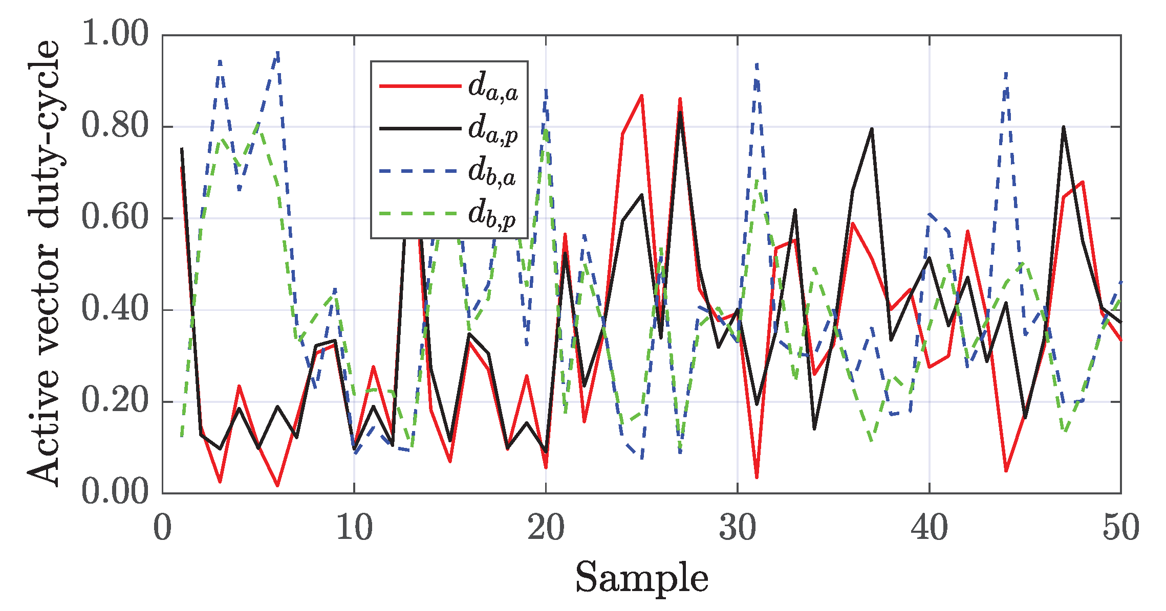
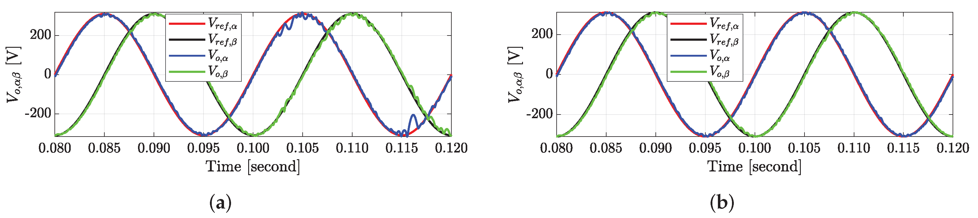
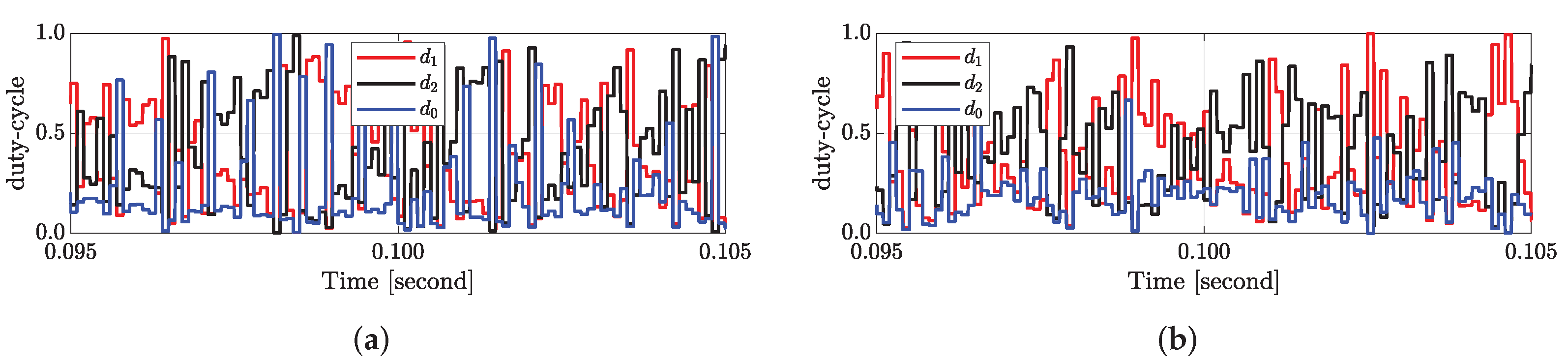
4. Simulation Results and Discussion
5. Conclusions
Author Contributions
Funding
Institutional Review Board Statement
Informed Consent Statement
Data Availability Statement
Conflicts of Interest
References
- Carrasco, J.M.; Franquelo, L.G.; Bialasiewicz, J.T.; Galván, E.; PortilloGuisado, R.C.; Prats, M.M.; León, J.I.; Moreno-Alfonso, N. Power-electronic systems for the grid integration of renewable energy sources: A survey. IEEE Trans. Ind. Electron. 2006, 53, 1002–1016. [Google Scholar] [CrossRef]
- Geldenhuys, J.M.; du Toit Mouton, H.; Rix, A.; Geyer, T. Model predictive current control of a grid connected converter with LCL-filter. In Proceedings of the 2016 IEEE 17th Workshop on Control and Modeling for Power Electronics (COMPEL), Trondheim, Norway, 27–30 June 2016; pp. 1–6. [Google Scholar] [CrossRef]
- Mohamed, I.S.; Zaid, S.A.; Abu-Elyazeed, M.F.; Elsayed, H.M. Classical methods and model predictive control of three-phase inverter with output LC filter for UPS applications. In Proceedings of the 2013 International Conference on Control, Decision and Information Technologies (CoDIT), Hammamet, Tunisia, 6–8 May 2013; pp. 483–488. [Google Scholar]
- Rodriguez, J.; Cortes, P. Predictive Control of Power Converters and Electrical Drives, 1st ed.; John Wiley & Sons: Hoboken, NJ, USA, 2012; Volume 40, Chapter 5; p. 181. [Google Scholar]
- Nauman, M.; Hasan, A. Efficient implicit model-predictive control of a three-phase inverter with an output LC filter. IEEE Trans. Power Electron. 2016, 31, 6075–6078. [Google Scholar] [CrossRef]
- Vazquez, S.; Rodriguez, J.; Rivera, M.; Franquelo, L.G.; Norambuena, M. Model predictive control for power converters and drives: Advances and trends. IEEE Trans. Ind. Electron. 2017, 64, 935–947. [Google Scholar] [CrossRef] [Green Version]
- Cortés, P.; Ortiz, G.; Yuz, J.I.; Rodríguez, J.; Vazquez, S.; Franquelo, L.G. Model predictive control of an inverter with output LC filter for UPS applications. IEEE Trans. Ind. Electron. 2009, 56, 1875–1883. [Google Scholar] [CrossRef]
- Alhasheem, M. Improvement of Transient Power Sharing Performance in Parallel Converter System and Microgrids. Ph.D. Thesis, Faculty of Engineering and Science, Aalborg University, Aalborg, Denmark, 2019; 91p. [Google Scholar]
- Aguirre, M.; Kouro, S.; Rojas, C.A.; Rodriguez, J.; Leon, J.I. Switching frequency regulation for fcs-mpc based on a period control approach. IEEE Trans. Ind. Electron. 2018, 65, 5764–5773. [Google Scholar] [CrossRef]
- Zhang, Y.; Liu, J.; Fan, S. On the inherent relationship between finite control set model predictive control and SVM-based deadbeat control for power converters. In Proceedings of the IEEE Energy Conversion Congress and Exposition (ECCE), Cincinnati, OH, USA, 1–5 October 2017; pp. 4628–4633. [Google Scholar] [CrossRef]
- Riveros, J.A.; Rivera, M.; Rodriguez, C.; Galea, M.; Buticchi, G.; Wheeler, P. Predictive Torque Control with Fixed Switching Frequency for Induction Motor Drives. In Proceedings of the IEEE International Conference on Industrial Technology (ICIT), Buenos Aires, Argentina, 26–28 February 2020; pp. 211–216. [Google Scholar] [CrossRef]
- Jiang, C.; Du, G.; Du, F.; Lei, Y. A Fast Model Predictive Control with Fixed Switching Frequency Based on Virtual Space Vector for Three-Phase Inverters. In Proceedings of the IEEE International Power Electronics and Application Conference and Exposition (PEAC), Shenzhen, China, 4–7 November 2018; pp. 1–7. [Google Scholar] [CrossRef]
- Rojas, F.; Kennel, R.; Cardenas, R.; Repenning, R.; Clare, J.C.; Diaz, M. A new space-vector-modulation algorithm for a three-level four-leg NPC inverter. IEEE Trans. Energy Convers. 2017, 32, 23–35. [Google Scholar] [CrossRef]
- Osman, I.; Xiao, D.; Alam, K.S.; Shakib, S.M.; Akter, M.P.; Rahman, M.F. Discrete Space Vector Modulation-Based Model Predictive Torque Control with No Suboptimization. IEEE Trans. Ind. Electron. 2020, 67, 8164–8174. [Google Scholar] [CrossRef]
- Guo, L.; Jin, N.; Gan, C.; Xu, L.; Wang, Q. An improved model predictive control strategy to reduce common-mode voltage for two-level voltage source inverters considering dead-time effects. IEEE Trans. Ind. Electron. 2019, 66, 3561–3572. [Google Scholar] [CrossRef]
- Alsofyani, I.M.; Lee, K.B. Improved Deadbeat FC-MPC Based on the Discrete Space Vector Modulation Method with Efficient Computation for a Grid-Connected Three-Level Inverter System. Energies 2019, 12, 3111. [Google Scholar] [CrossRef] [Green Version]
- De Bosio, F.; de Souza Ribeiro, L.A.; Freijedo, F.D.; Pastorelli, M.; Guerrero, J.M. Effect of state feedback coupling and system delays on the transient performance of stand-alone VSI with LC output filter. IEEE Trans. Ind. Electron. 2016, 63, 4909–4918. [Google Scholar] [CrossRef] [Green Version]
- Zhang, Y.; Qu, C. Model Predictive Direct Power Control of PWM Rectifiers Under Unbalanced Network Conditions. IEEE Trans. Ind. Electron. 2015, 62, 4011–4022. [Google Scholar] [CrossRef]
- Alhasheem, M.; Blaabjerg, F.; Davari, P. Davari, Performance Assessment of Grid Forming Converters Using Different Finite Control Set Model Predictive Control (FCS-MPC) Algorithms. Appl. Sci. 2019, 9, 3513. [Google Scholar] [CrossRef] [Green Version]
- Cortés, P.; Kazmierkowski, M.P.; Kennel, R.M.; Quevedo, D.E.; Rodríguez, J. Predictive control in power electronics and drives. IEEE Trans. Ind. Electron. 2008, 55, 4312–4324. [Google Scholar] [CrossRef]
- Rivera, M. A new predictive control scheme for a VSI with reduced common mode voltage operating at fixed switching frequency. In Proceedings of the IEEE 5th International Conference on Power Engineering, Energy and Electrical Drives (POWERENG), Riga, Latvia, 11–13 May 2015; pp. 617–622. [Google Scholar] [CrossRef]
- Pinto, J.O.; Bose, B.K.; Da Silva, L.B.; Kazmierkowski, M.P. A neural network based space vector PWM controller for voltage-fed inverter induction motor drive. IEEE Trans. Ind. Electron. 2000, 36, 1628–1636. [Google Scholar]
- Chen, J.; Chen, Y.; Tong, L.; Peng, L.; Kang, Y. A Back propagation Neural Network-Based Explicit Model Predictive Control for DC–DC Converters with High Switching Frequency. IEEE J. Emerg. Sel. Top. Power Electron. 2020, 8, 2124–2142. [Google Scholar] [CrossRef]
- Wang, D.; Yin, X.; Tang, S.; Zhang, C.; Shen, Z.J.; Wang, J.; Shuai, Z. A Deep Neural Network Based Predictive Control Strategy for High Frequency Multilevel Converters. In Proceedings of the IEEE Energy Conversion Congress and Exposition, Portland, OR, USA, 23–27 September 2018; pp. 2988–2992. [Google Scholar]
- Mohamed, I.S.; Rovetta, S.; Do, T.D.; Dragicević, T.; Diab, A.A.Z. A Neural-Network-Based Model Predictive Control of Three-Phase Inverter with an Output LC Filter. IEEE Access 2019, 7, 124737–124749. [Google Scholar] [CrossRef]
- Novak, M.; Dragicevic, T. Supervised imitation learning of finite set model predictive control systems for power electronics. IEEE Trans. Ind. Electron. 2020, 68, 1717–1723. [Google Scholar] [CrossRef]
- Lucia, S.; Navarro, D.; Karg, B.; Sarnago, H.; Lucia, O. Deep Learning-based Model Predictive Control for Resonant Power Converters. IEEE Trans. Ind. Inform. 2020, 17, 409–420. [Google Scholar] [CrossRef] [Green Version]
- Dragičević, T.; Novak, M. Weighting Factor Design in Model Predictive Control of Power Electronic Converters: An Artificial Neural Network Approach. IEEE Trans. Ind. Electron. 2018, 66, 2124–2142. [Google Scholar]
- Bakeer, A.; Magdy, G.; Chub, A.; Bevrani, H. A sophisticated modeling approach for photovoltaic systems in load frequency control. Int. J. Electr. Power Energy Syst. 2022, 134, 107330. [Google Scholar] [CrossRef]
- Awad, M.; Qasrawi, I. Enhanced RBF neural network model for time series prediction of solar cells panel depending on climate conditions (temperature and irradiance). Neural Comput. Appl. 2016, 30, 1757–1768. [Google Scholar] [CrossRef]


| Scenario | [mH] | [F] | R [] | L [mH] | [s] |
|---|---|---|---|---|---|
| 1 | 1 | 40 | 10 | 1 | 40 |
| 2 | 1 | 55 | 11 | 2 | 40 |
| 3 | 0.85 | 50 | 15 | 3 | 60 |
| 4 | 0.50 | 55 | 10 | 4 | 35 |
| 5 | 0.75 | 35 | 12 | 5 | 40 |
| 6 | 0.90 | 45 | 25 | 6 | 50 |
| 7 | 1 | 40 | 10 | 10 | 50 |
| Parameter | Symbol | Value |
|---|---|---|
| Input voltage | 700 V | |
| Filter inductance | 2 mH | |
| Filter capacitance | 50 μF | |
| Switching frequency | 10 kHz | |
| Sampling time | 100 μs | |
| Nominal RMS output voltage (L-L) | 380 V |
Publisher’s Note: MDPI stays neutral with regard to jurisdictional claims in published maps and institutional affiliations. |
© 2022 by the authors. Licensee MDPI, Basel, Switzerland. This article is an open access article distributed under the terms and conditions of the Creative Commons Attribution (CC BY) license (https://creativecommons.org/licenses/by/4.0/).
Share and Cite
Bakeer, A.; Alhasheem, M.; Peyghami, S. Efficient Fixed-Switching Modulated Finite Control Set-Model Predictive Control Based on Artificial Neural Networks. Appl. Sci. 2022, 12, 3134. https://0-doi-org.brum.beds.ac.uk/10.3390/app12063134
Bakeer A, Alhasheem M, Peyghami S. Efficient Fixed-Switching Modulated Finite Control Set-Model Predictive Control Based on Artificial Neural Networks. Applied Sciences. 2022; 12(6):3134. https://0-doi-org.brum.beds.ac.uk/10.3390/app12063134
Chicago/Turabian StyleBakeer, Abualkasim, Mohammed Alhasheem, and Saeed Peyghami. 2022. "Efficient Fixed-Switching Modulated Finite Control Set-Model Predictive Control Based on Artificial Neural Networks" Applied Sciences 12, no. 6: 3134. https://0-doi-org.brum.beds.ac.uk/10.3390/app12063134