
Computational Wear Prediction of TKR with Flatback Deformity during Gait


1
Department of Biomedical Engineering, Dongguk University, Goyang 10326, Korea
2
Research Institute for Commercialization of Biomedical Convergence Technology, Dongguk University, Goyang 10326, Korea
*
Author to whom correspondence should be addressed.
Appl. Sci. 2022, 12(7), 3698; https://0-doi-org.brum.beds.ac.uk/10.3390/app12073698
Submission received: 11 January 2022
/
Revised: 23 March 2022
/
Accepted: 4 April 2022
/
Published: 6 April 2022
(This article belongs to the Special Issue Biomechanical and Biomedical Factors of Knee Osteoarthritis)
Abstract
:Loss of lumbar lordosis in flatback patients leads to changes in the walking mechanism like knee flexion. Such variations in flatback patients are predicted to alter the characteristics of total knee replacement (TKR) contact, so their TKR will show different wear characteristics with a normal gait. However, the relevant study is limited to predicting the wear depth of TKR for normal gait mechanisms or collecting and analyzing kinematic data on flatback gait mechanisms. The objective of this study was to compare wear in TKR of flatback patients with people without flatback syndrome. The main difference between the normal gait mechanism and the flat back gait mechanism is the knee flexion remain section and the tendency to change the vertical force acting on the knee. Thus, in this paper, A finite element-based computational wear simulation for the gait cycle using kinematic data for normal gait and flat gait were performed, and substituting the derived contact pressure and slip distance into the Archard formula, a proven wear model, wear depth was predicted. The FE analysis results show that the wear volume in flatback patients is greater. The results obtained can provide guidance on the TKR design to minimize wear on the knee implant for flatback patients.
1. Introduction
Flatback syndrome results in muscular pain in the upper back and lower cervical area, knee pain, and inability to stand erect, and is also referred to as “fixed sagittal imbalance” [1,2]. Flatback syndrome is diagnosed as follows. A plumb line is dropped vertically from the center of the C7 body, and the horizontal linear distance between the plumb line and the posterior-superior part of the sacral end plate is measured. If this distance is more than ±3 cm, it is judged that the spine has deformed [3,4]. Among the known symptoms associated with flatback syndrome is difficulty in maintaining an upright posture is due to loss of lumbar lordosis [2]. As a result, the body compensates for the posture in various ways to maintain the correct posture, one of which is the flexion of the knee as shown in Figure 1. However, this mechanism to compensate for posture through knee flexion increases the load on the knee joint and causes the progression to knee arthritis, causing knee pain [5].
Limits in knee extension and knee pain due to continuous knee flexion can be improved by total knee replacement (TKR) [5]. As shown in Figure 2, a knee artificial joint consists of the femoral components and tibial insert. The femoral component is a metal that is applied to the distal ends of the femur, and the tibial insert is a specially made plastic plate that acts as cartilage inserted to reduce friction. The tibial insert is prone to wear as it absorbs shocks and allows the knee joints to move smoothly during lower limb exercise. The wear of the tibial insert has been regarded as the most important cause of complications after TKR, and many studies have been conducted on this [6,7,8]. However, due to the loss of lumbar lordosis, flatback patients are predicted to have different wear characteristics from normal gait because the gait mechanism is different from that of people without flatback syndrome, and changes the contact characteristics of the knee artificial joint.
Currently, related research can confirm the study on the wear of the knee artificial joint in the normal gait mechanism [6,8,10,11,12,13,14,15,16] or study the study on the compensation mechanism of the spine and knee by collecting and analyzing kinematic data during gait of flatback patients [2,5,17,18,19,20,21]. These researchers have presented the results of their study, such as a comparison of wear volume according to materials used for friction surface of the knee artificial joint, a comparison of wear volume of the knee artificial joint by experiment and computational simulation, a comparison of wear volume of the knee artificial joint by ISO standards, and an analysis of the effects of loss of lumbar lordosis on the knee in flatback patients by comparing the kinematic data of people without flatback syndrome. However, there has been no study to predict the wear on the knee artificial joint considering the gait mechanism of the flatback patients that is different from that of people without flatback syndrome. Therefore, a comparative study was conducted on the wear characteristics of the gait mechanism of flatback patients, which is different from the gait mechanism of people without flatback syndrome, and it is necessary to present this result as a design guideline for knee artificial joint in flatback patients.
The purpose of this study is to predict the wear characteristics of the knee artificial joint in normal gait mechanism and flatback gait mechanism. To obtain the wear characteristics in flatback patients due to differences from normal gait mechanisms, we used the finite element (FE) method in this study. Performing a wear experiment requires a lot of time and cost, so it is more efficient in terms of time and cost to predict and analyze knee artificial joint wear through computational simulation using finite element analysis. After the creation of the finite element model, finite element analysis was performed by applying constraint and loading conditions for Modified ISO 14243-3 in the case of people without flatback syndrome and for experimental results of previous research [15] in the case of flatback patients. Through this analysis, contact pressure and sliding distance for one gait cycle were obtained, and the wear depth was calculated by using Archard’s Law [22,23,24]. The wear in the flatback patient’s gait mechanism and the wear in the normal gait mechanism were compared by the wear area and contact area results after 5,000,000 cycles. The study about wear can contribute to guiding TKR design and positioning to reduce wear for flatback patients.
This paper consists of five sections. Following this section, a finite element model is performed to derive the contact pressure distribution of the knee artificial joint. Then, Archard’s Law, which derives the wear depth using the obtained contact pressure, is introduced, and the process for deriving the wear depth of the artificial joint bearing after 5,000,000 cycles is presented. In the third section, numerical results obtained by employing the finite element analysis model are exhibited and the accuracy of the results is verified by comparing the actual experimental results. Furthermore, we compare and analyze the contact pressure, maximum sliding distance, wear depth, and wear area of the normal gait mechanism and the flat gait mechanism. In the fourth section, the discussions related to the results are given. In particular, the effect of the difference in contact pressure very during the gait cycle due to the difference in the gait mechanism on wear was analyzed. Finally, conclusions are made in the final section.
2. Methods
2.1. Finite Element Analysis Model
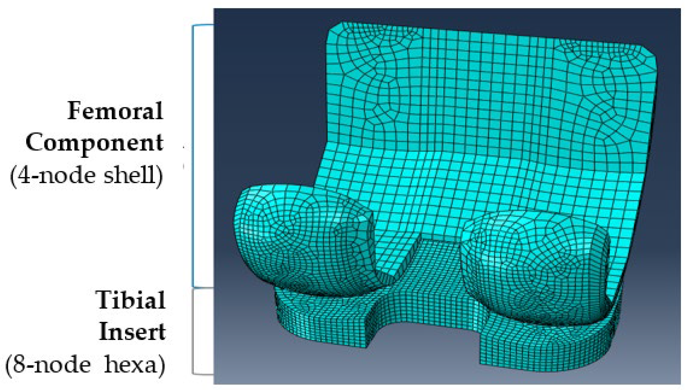
The 3D CAD model of the femoral component and tibial insert of the knee artificial joint was made using SolidWorks 2020 (Solidworks Corp., Waltham, MA, USA). The femoral component was modeled as a rigid body with 4-node-shell elements and the tibial insert was modeled with 8-node hexahedral elements (See Figure 3). Meshing, analysis and post-processing were performed using ABAQUS 2016 (Abaqus, Inc., Johnston, RI, USA). Ultra-high molecular weight polyethylene (UHMWPE) was applied as the material of the tibial insert. UHMWPE material was modeled using the J-2 Plasticity model with a density of 9.4 × 10⁻¹⁰ tonne/mm3, an elastic modulus of 1051 MPa and a Poisson’s ratio of 0.46. The stress–strain data used in the J-2 Plasticity model are shown in Table 1 [15].
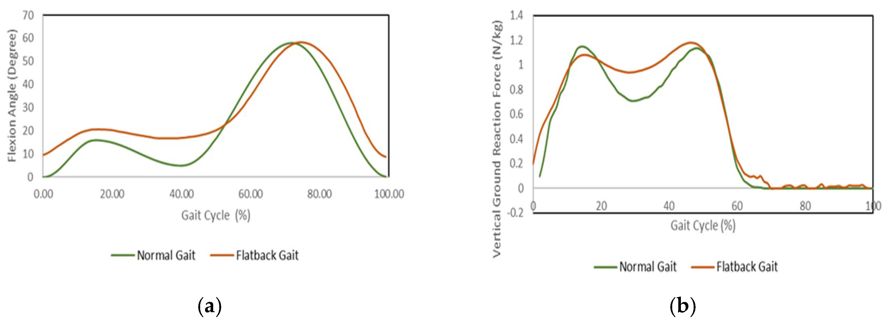
A penalty-based method was applied to define the contact between the femoral component and the tibial insert of the knee artificial joint. For the efficiency of the computational simulation, the femoral component was modeled as a rigid body [8,10]. However, the tibial insert was modeled as a flexible body to consider wear and deformation. The friction coefficient was set to 0.04, which is the result obtained in the experiment of the previous study [11,14,15]. To apply the motion of the knee artificial joint during the gait cycle (see Figure 4), in the normal gait mechanism, the knee flexion–extension angle (see Figure 5a), anterior–posterior displacement (see Figure 5d), and adduction–abduction angle (see Figure 5c) applied the conditions of the modified ISO 14243-3 [14]. Furthermore, in the flatback gait mechanism, the knee flexion–extension angle (see Figure 6a, red line) applied the kinematic data obtained through the experiment on flatback patients in a previous study [2], but the anterior–posterior displacement (see Figure 5d) and adduction–abduction angle (see Figure 5d) applied the same data as for the normal gait mechanism. For the vertical force acting on the knee artificial joint, experimental data (see Figure 6b) from a previous study [2] were applied for both gait mechanisms. The anterior–posterior displacement and adduction–abduction angle data for the flatback gait mechanism could not be confirmed in a related previous study. Furthermore, a previous study comparing the kinematic data during normal gait and flatback gait also focused on the knee flexion–extension angle and the vertical force acting on the knee. Therefore, it can be inferred that the application of the data of normal gait case to the anterior–posterior displacement and adduction–abduction angle of the flatback gait case does not have a significant effect on the comparison of the two gait mechanisms.
The boundary conditions and loading conditions were set according to ISO 14243-3 [26]. As shown in Figure 7, IE rotation (see Figure 5c) and AP displacement (see Figure 5d) were applied to the tibial insert as boundary conditions at a reference point located at the center of mass of the tibial insert. Medial/lateral (ML) displacement of the tibial insert was left free, and flexion–extension rotation of the tibial insert was fixed. Flexion–extension rotation was applied to the femoral component as boundary conditions and other directional degrees of freedom were fixed. All displacement conditions given to the femoral component were given to the rigid reference point of the femoral component. The loading point on the tibial insert was offset to the medial side by a distance of 0.07 times the width of the tibial insert according to ISO 14243-3 [26]. The summary of the boundary conditions given to the femoral component and tibial insert can be seen in Figure 7.
Since this study is a comparison of the distribution of contact pressure and wears characteristics in the normal gait mechanism and in the flatback gait mechanism, the experimental result values from the previous study [2] that obtained the load condition of the flatback gait mechanism were also applied to the load condition in the normal gait mechanism. The previous experimental result values are given as standardized vertical ground reaction force values. Since the vertical ground reaction force is proportional to the axial compression force across the knee joint, it was used by multiplying the appropriate value to fit the load conditions in ISO 14243-3 [26] (see Figure 5b).
The major difference between the normal gait mechanism and the flatback gait mechanism is that the knee flexion and vertical reaction force [2,26] are maintained continuously (see Figure 6). Since the vertical ground reaction force approaches indirectly in proportion to the axial compressive force across the knee joint, it can be inferred that the axial force applied to the knee is also maintained continuously in the flatback gait mechanism. Furthermore, this seems to affect the wear on the knee artificial joint.
2.2. Wear Prediction by Using Archard’s Law
To calculate the wear depth on the tibial insert, it was numerically formulated using Archard’s Law. Archard’s Law is an equation introduced to evaluate the linear wear depth perpendicular to the wear surface between two metal surfaces sliding relative to each other. The formula known as Archard’s Law of wear is as follows [22]:
where H is the linear wear depth, Kw is an experimentally determined wear factor, p is contact pressure, and S is the sliding distance. For the wear factor Kw, a value of 2.64 × 10⁻⁷ mm3/Nm is generally used in a previous study [11].
In the formula mentioned above, the factor that most influences the wear depth is the contact pressure [13,23]. Therefore, in this study, the wear depth and wear area will be predicted through the magnitude and distribution of the contact pressure for one gait cycle.
The process for deriving the wear depth was carried out according to the sequence shown in Figure 8. After performing a finite element nonlinear transient analysis for one gait cycle, the contact pressure and sliding distance are obtained from the output file, respectively. In the finite element software ABAQUS used in this paper, the contact pressure and sliding distance is obtained from CPRESS and CSLIP of the field output file, which is the ABAQUS result file. where CSLIP is the sum of the tangential distances of the node of the tibial insert including the slave surface. Therefore, for every time-step, the INCSLIP value, which is the value of subtracting the CSLIP of the previous time-step from the CSLIP of the current time-step, is applied. By substituting the obtained contact pressure and sliding distance into Equation (1), the wear depth at each node was derived, and the wear depth was multiplied by 500,000. The position of each node was updated by the derived wear depth after 500,000 cycles, and the worn contact surface shape was updated. By repeating this process 10 times, the wear depth after 5,000,000 gait cycles can be derived. Additionally, the position update cycle reflecting the wear depth of each node was applied to the results of a previous study that the result of updating node position every 500,000 cycles has convergence [10].
3. Results
3.1. Model Validation
A convergence study was performed to find the optimum mesh size in the tibial insert (see Figure 9). Mesh convergence was selected as the mesh size when the maximum contact pressure values were all within 5% of the following two mesh sizes [27,28,29,30,31]. The average mesh size suitable for that criterion was 1.1 mm and the number of elements was 16,376. The mesh size of the face where the femoral component contacts the tibial insert was the same as the mesh size of the tibial insert and the number of elements in the femoral part was 7102.
To verify the wear simulation model performed by finite element analysis, the wear simulation results were compared with the wear results of a previous study [15]. For the finite element analysis performed, the load and displacement conditions were applied to the standard of ISO 14243-3:2004 [26] to match the actual test conditions, and the results of the wear rate at 4,000,000 cycles were derived and compared. The wear rate was obtained by subtracting the mass of the tibial insert after 4,000,000 cycles of analysis from the mass of the tibial insert before performing the wear analysis. As shown in Table 2, the wear rate (8.26 mg/MC) of the finite element analysis performed in this study and the wear rate (8.66 mg/MC) of the finite element analysis performed in the previous study [15] show similar results. Therefore, it can be judged that the reliability of the model proposed in this study has been verified. However, this wear rate is larger than the experimental wear rate (2.96~7.32 mg/MC) of the previous study. This difference can be explained by not considering the viscoelastic effect in the material model used in this study. Considering the viscoelastic effect of a knee artificial joint using UHMWPE (ultra high molecular weight polyethylene) material, it was found that the contact pressure decreased by more than 10% when the compressive force was continued [32]. Since the wear depth is proportional to the contact pressure, considering the viscoelastic effect of the UHMWPE material, the wear rate will decrease as the wear depth decreases. However, since the purpose of this study is to analyze the difference in wear trends according to other gait characteristics rather than to derive an accurate wear rate, the viscoelastic effect was not considered for the simplification of the analysis model and faster analysis time.
Additionally, in order to verify the finite element model, the graph of maximum contact pressure during one gait cycle was compared with the graph of the results of a previous study [11,16,33]. The axial force applied to the presented FE model was used the modified ISO 14243-3 [14] (see Figure 5b). As shown in Figure 10, the maximum contact pressure tendency in the previous study showed that the peak value appeared twice before the gait cycle of 20%. Next, the peak value appeared immediately after the gait cycle of 40%. Finally, decreases and the low value were maintained after the gait cycle of 60%. The maximum contact pressure graph during one gait cycle obtained as the analysis results of this study coincided with the position of the pressure peak points and the position where the value decreased compared to the graph of the maximum contact pressure of the previous study. Above all, in the graph of the previous study, the section where the value decreased significantly after 60% of the gait cycle was also well shown in the graph of the analysis result of this study. This study does not aim to verify whether the finite element model can replace the experimental model, but to compare the wear characteristics of knee artificial joints in normal and flatback gait mechanisms. Therefore, it is judged that the finite element model proposed in this study is reliable in comparing the wear characteristics of the knee artificial joint according to the gait mechanism.
3.2. Comparison of Contact Pressure of Normal Gait Mechanism and Flatback Gait Mechanism
Figure 11 shows the graph of the maximum contact pressure in one gait cycle for the normal gait mechanism and flatback gait mechanism. The major difference between the two gait mechanisms was that in the section after 20% of the gait cycle, there was a section in which the maximum contact pressure decreased in the normal gait mechanism, but the flatback gait mechanism did not exist. In addition, the magnitude of the maximum contact pressure at the start of the gait cycle had a value of 15.89 MPa for the normal gait mechanism, while 23.80 MPa for the flatback gait mechanism was higher than that of the normal gait mechanism. Therefore, during one gait cycle, flatback patients are expected to have a greater depth of wear because they receive higher contact pressure than normal.
Figure 12 shows the contact pressure distribution of the tibial insert in one gait cycle for the normal gait mechanism and flatback gait mechanism. The contact point was similar in both gait mechanisms, but the contact area showed a difference between the two mechanisms. Until the 60% gait cycle, the contact area of the flatback gait mechanism was 10–20% greater than that of the normal gait mechanism. However, after the 60% gait cycle, on the contrary, the normal gait showed slightly larger values than the flatback gait. This phenomenon can be inferred that the gait mechanism with a greater magnitude of the maximum contact pressure in each phase of the compared gait cycle presses the contact surface with a greater force, which resulted in a greater contact area.
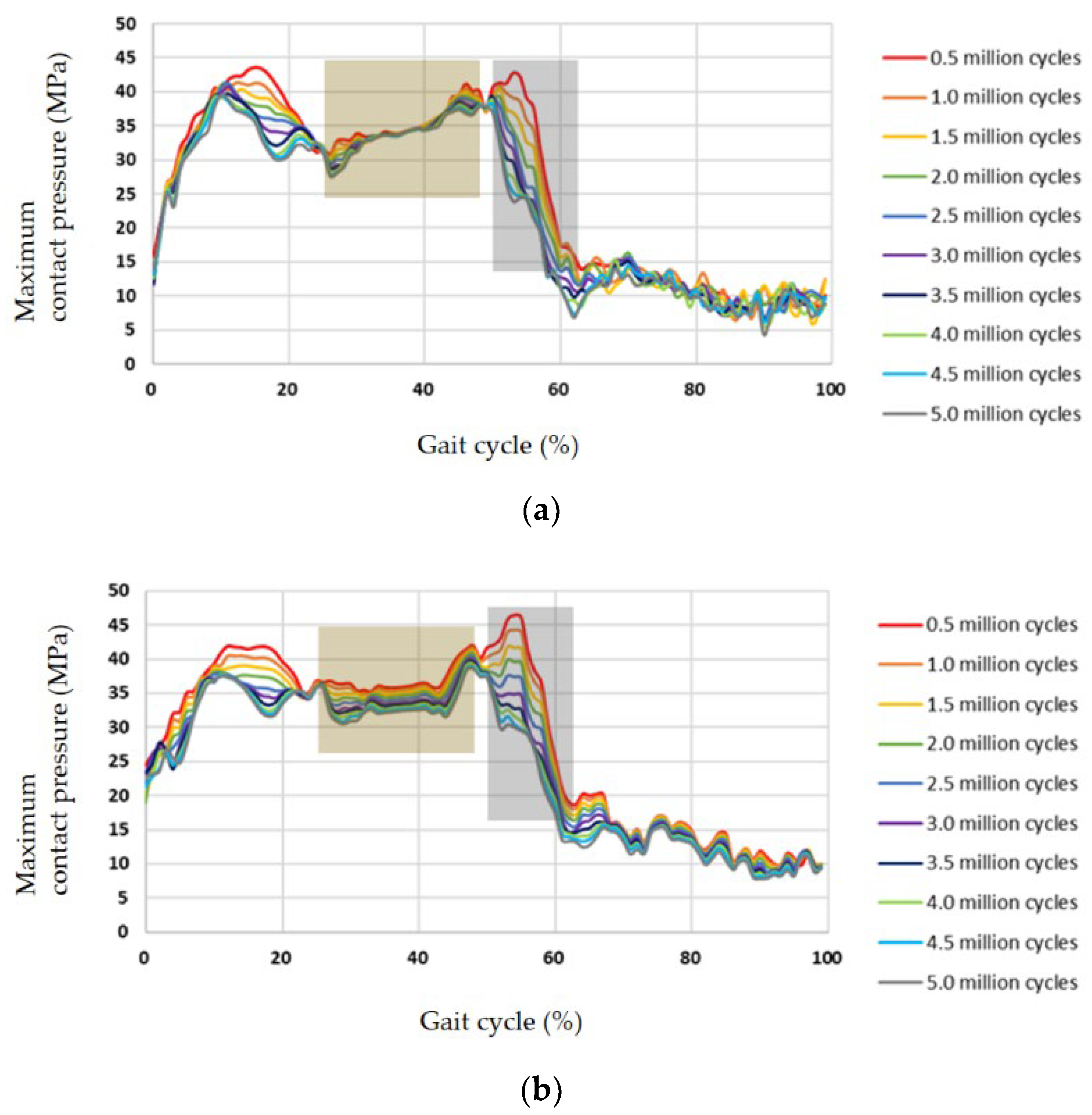
In the wear simulation, the contact surface shape of the tibial insert is updated at intervals of 500,000 gait cycles. The maximum contact pressure variation during one gait cycle due to the contact surface shape updated every 500,000 cycles is shown in Figure 13. Overall, as the gait cycle increases, the contact area increases due to wear in both the normal gait mechanism and the flatback gait mechanism, and the maximum contact pressure tends to decrease. However, in the 25–50% gait cycle, the two gait mechanisms show different aspects. In this section, the maximum contact pressure in the normal gait mechanism did not decrease significantly even when the number of gait cycles increased, whereas in the flatback gait mechanism, the maximum contact pressure decreased remarkably as the gait cycles increased. This phenomenon can be predicted that more wear occurs on the contact surface of the knee artificial joint in the case of flatback patients in the 25–50% gait cycle.
In order to confirm the wear depth in one gait cycle, the graph of the maximum wear depth after 5,000,000 cycles was compared. As shown in Figure 14, the peak value of the maximum wear depth was greater in the normal gait mechanism, but the tendency to maintain the maximum wear depth during the gait cycle was greater in the flatback gait mechanism. The average value of the maximum wear depth during one gait cycle was 1.7953 × 10⁻⁹ mm for the normal gait mechanism and 1.8146 × 10⁻⁹ mm for the flatback gait mechanism, and there was no significant difference. However, this graph can find meaning in predicting the wear volume for each gait cycle section. The peak value of the maximum wear depth appeared just before 60% of the gait cycle for both gait mechanisms, and generally maintained a large value after 50% of the gait cycle. In the case of the normal gait mechanism, the maximum wear depth was greater than that of the flatback gait mechanism in the 0–20% gait cycle. Furthermore, in the case of the flatback gait mechanism, the maximum wear depth was greater than that of the normal gait mechanism in the 20–40% gait cycle.
4. Discussion
The purpose of this study was to compare the maximum contact pressure, distribution of contact pressure and wear depth from the flatback gait mechanism against the normal gait mechanism. Unlike the normal gait mechanism, the flatback gait mechanism maintains the knee flexion and maintains the vertical force applied to the knee, so it can be expected that the wear characteristics of the two gait mechanisms will be different.
When the finite element analysis was performed for 5,000,000 gait cycles, the maximum contact pressure of the flatback gait mechanism decreased as the cycles increased in the 25–50% gait cycle section, unlike the normal gait mechanism (see Figure 13). This reduction in contact pressure causes more contact pressure to be applied to the tibia insert in a specific gait section, resulting in more wear. It can be inferred that the generated wear increases the conformity of the shape of the joint contact surface, so the contact area is widened and the contact pressure is dispersed, resulting in a decrease in the maximum contact pressure. In the maximum wear depth graph, it was confirmed that the maximum wear depth of the flatback gait mechanism was generally greater than the wear depth of the normal gait mechanism in the 25–50% gait cycle section (see Figure 14).
For the contact pressure distribution, it is important to analyze the difference in the contact area rather than the contact pressure distribution point. The contact pressure distribution area was larger in the case of the flatback gait mechanism, and it can be seen that the contact pressure was also greater in this gait cycle. From this result, we can infer that the increase in the contact pressure region is not the effect of distributing the load, but is due to the increase in the applied contact pressure. Since the simultaneous increase of the contact pressure and the contact area can be judged as an increase in the wear volume, it can be predicted that the wear volume will be greater in the flatback gait mechanism. In relation to this, as shown in Figure 13, the large decrease of the maximum contact pressure in the case of flatback gait mechanism in the 25–45% gait cycle can be analyzed as a phenomenon in which the load is distributed because the contact area is widened due to wear even when the same load is applied.
The maximum wear depth showed a generally great value after 50% of the gait cycle, just before the swing phase for both gait mechanisms (see Figure 14). This can be thought of as a large increase in the maximum wear depth because the sliding distance increases when the foot is off the ground and the joint rotates freely. In addition, as the maximum wear depth is greater in the 20–40% gait cycle for the flatback gait mechanism, the fact that the maximum wear depth, which is directly related to the wear volume, shows different trends in the two gait mechanisms can be considered as different wear points. Due to this, it can be expected that the shape of the deformed tibial insert and the femoral component will appear differently for the two gait mechanisms. One of the ways to reduce the wear of the knee artificial joint is to increase the conformity of the tibial insert and the femoral component [34,35]. Therefore, if you increase the conformity of the knee joint artificial joint, for this reason, the contact pressure can be reduced, so it can be inferred that the wear depth and the wear volume will decrease. In conclusion, it is necessary to predict wear patterns in consideration of gait characteristics different from those of normal persons in order to improve the conformity of the femur and bearing during TKR (total knee arthroplasty) in the case of flatback patients.
5. Conclusions
In this study, using the finite element method, the wear phenomenon of a knee artificial joint was compared with the flatback gait mechanism and the normal gait mechanism and analyzed according to the gait cycle. For the load and boundary conditions applied to the finite element analysis, the data of ISO 14243-3:2004 were used for the normal gait mechanism, and the kinematic data of the flatback patient obtained through the experiment [15] were used for the flatback gait mechanism. As a result of the finite element analysis, the maximum contact pressure and the sliding distance of the wear surface during one gait cycle were derived, and the wear depth was calculated using these results and Archard’s law. The flatback gait mechanism and the normal gait mechanism showed differences in the magnitude and distribution of the maximum contact pressure. During one gait cycle, a zone in which the maximum contact pressure decreased is observed in the normal gait mechanism but in the flatback gait mechanism, no zone of decreasing maximum contact pressure appeared and a tendency to maintain a high value was observed. The difference in these results could be predicted to have a greater effect of wear on the knee artificial joint in the flatback gait mechanism than in the normal gait mechanism. Therefore, more research is needed on the wear of the knee artificial joint using the gait mechanism of flatback patients with an inequality that is different from the normal gait mechanism.
This paper has a limitation in that the wear analysis was performed by applying the anterior–posterior displacement and adduction–abduction angular displacement of the flatback patients identically to the normal gait data. Therefore, in a future study, the anterior–posterior displacement and adduction–abduction angular displacement of flatback gait mechanism be obtained for the experiment, and, if this result is applied to the results of flatback patients, it is thought that it will be possible to identify the difference in wear characteristics more accurately.
Author Contributions
Conceptualization, S.M.K. and H.S.L.; Data curation, H.K.L.; Formal analysis, H.K.L.; Funding acquisition, H.S.L.; Investigation, S.M.K.; Methodology, H.S.L.; Software, H.K.L.; Supervision, S.M.K.; Visualization, H.K.L.; Writing—original draft, H.K.L.; Writing—review and editing, H.S.L. All authors have read and agreed to the published version of the manuscript.
Funding
This research was funded by the Ministry of Education, Korea, grant number NRF-2020R1I1A1A01068607. This work was supported by Research Staff Program of the Ministry of Education, Republic of Korea. (NRF-2020R1I1A1A01068607).
Institutional Review Board Statement
Not applicable.
Informed Consent Statement
Patient consent was waived due to this study used only the human body data presented in the references.
Conflicts of Interest
The authors declare no conflict of interest.
References
- Lu, D.C.; Chou, D. Flatback Syndrome. Neurosurg. Clin. N. Am. 2007, 18, 289–294. [Google Scholar] [CrossRef] [PubMed]
- Sarwahi, V.; Boachie-Adjei, O.; Backus, S.I.; Taira, G. Characterization of Gait Function in Patients With Postsurgical Sagittal (Flatback) Deformity: A Prospective Study of 21 Patients. Spine 2002, 27, 2328–2337. [Google Scholar] [CrossRef] [PubMed]
- Berven, S.H.; Deviren, V.; Smith, J.A.; Emami, A.; Hu, S.S.; Bradford, D.S. Management of Fixed Sagittal Plane Deformity : Results of the Transpedicular Wedge Resection Osteotomy. Spine 2001, 26, 2036–2043. [Google Scholar] [CrossRef] [PubMed]
- Potter, B.K.; Lenke, L.G.; Kuklo, T.R. Prevention and management of iatrogenic flatback deformity. J. Bone Jt. Surg. 2004, 86, 1793–1808. [Google Scholar] [CrossRef] [Green Version]
- Oshima, Y.; Watanabe, N.; Iizawa, N.; Majima, T.; Kawata, M.; Takai, S. Knee-Hip-Spine Syndrome: Improvement in Preoperative Abnormal Posture following Total Knee Arthroplasty. Adv. Orthop. 2019, 2019, 8484938. [Google Scholar] [CrossRef]
- Netter, J.; Hermida, J.; Flores-Hernandez, C.; Steklov, N.; Kester, M.; D’Lima, D.D. Prediction of Wear in Crosslinked Polyethylene Unicompartmental Knee Arthroplasty. Lubricants 2015, 3, 381–393. [Google Scholar] [CrossRef]
- Fregly, B.J.; Sawyer, W.; Harman, M.K.; Banks, S. Computational wear prediction of a total knee replacement from in vivo kinematics. J. Biomech. 2005, 38, 305–314. [Google Scholar] [CrossRef]
- Kang, K.-T.; Son, J.; Kim, H.-J.; Baek, C.; Kwon, O.-R.; Koh, Y.-G. Wear predictions for UHMWPE material with various surface properties used on the femoral component in total knee arthroplasty: A computational simulation study. J. Mater. Sci. Mater. Electron. 2017, 28, 105. [Google Scholar] [CrossRef]
- Geetha, M.; Singh, A.K.; Asokamani, R.; Gogia, A.K. Ti based biomaterials, the ultimate choice for orthopaedic implants—A review. Prog. Mater. Sci. 2009, 54, 397–425. [Google Scholar] [CrossRef]
- Knight, L.A.; Pal, S.; Coleman, J.C.; Bronson, F.; Haider, H.; Levine, D.L.; Taylor, M.; Rullkoetter, P.J. Comparison of long-term numerical and experimental total knee replacement wear during simulated gait loading. J. Biomech. 2007, 40, 1550–1558. [Google Scholar] [CrossRef]
- Abdelgaied, A.; Liu, F.; Brockett, C.; Jennings, L.; Fisher, J.; Jin, Z. Computational Wear Prediction of Artificial Knee Joints Based on a New Wear Law and Formulation. J. Biomech. 2011, 44, 1108–1116. [Google Scholar] [CrossRef] [PubMed]
- Pal, S.; Haider, H.; Laz, P.J.; Knight, L.A.; Rullkoetter, P.J. Probabilistic computational modeling of total knee replacement wear. Wear 2008, 264, 701–707. [Google Scholar] [CrossRef]
- Noh, T.-H.; Chun, H.-J. Analysis of Contact Pressure for Material Combination in Unicompartmental Knee Implant. J. Comput. Struct. Eng. Inst. Korea 2018, 31, 23–29. [Google Scholar] [CrossRef]
- Wang, X.-H.; Zhang, W.; Song, D.-Y.; Li, H.; Dong, X.; Zhang, M.; Zhao, F.; Jin, Z.-M.; Cheng, C.-K. The impact of variations in input directions according to ISO 14243 on wearing of knee prostheses. PLoS ONE 2018, 13, e0206496. [Google Scholar] [CrossRef] [PubMed] [Green Version]
- Mell, S.P.; Fullam, S.; A Wimmer, M.; Lundberg, H.J. Finite element evaluation of the newest ISO testing standard for polyethylene total knee replacement liners. Proc. Inst. Mech. Eng. Part H J. Eng. Med. 2018, 232, 545–552. [Google Scholar] [CrossRef] [PubMed]
- Willing, R.; Kim, I.Y. Three dimensional shape optimization of total knee replacements for reduced wear. Struct. Multidiscip. Optim. 2009, 38, 405–414. [Google Scholar] [CrossRef]
- Murata, Y.; Takahashi, K.; Yamagata, M.; Hanaoka, E.; Moriya, H. The Knee-Spine Syndrome: Association Between Lumbar Lordosis and Extension of the Knee. J. Bone Jt. Surg Br. 2003, 85, 95–99. [Google Scholar] [CrossRef]
- Haddas, R.; Belanger, T. Clinical Gait Analysis on a Patient Undergoing Surgical Correction of Kyphosis from Severe Ankylosing Spondylitis. Int. J. Spine Surg. 2017, 11, 18. [Google Scholar] [CrossRef] [Green Version]
- Hirose, D.; Ishida, K.; Nagano, Y.; Takahashi, T.; Yamamoto, H. Posture of the trunk in the sagittal plane is associated with gait in community-dwelling elderly population. Clin. Biomech. 2004, 19, 57–63. [Google Scholar] [CrossRef]
- Chow, S.B.; Moffat, M. Relationship of Thoracic Kyphosis to Functional Reach and Lower-Extremity Joint Range of Motion and Muscle Length in Women with Osteoporosis or Osteopenia: A Pilot Study. Top. Geriatr. Rehabil. 2004, 20, 297–306. [Google Scholar] [CrossRef]
- Tauchi, R.; Imagama, S.; Muramoto, A.; Tsuboi, M.; Ishiguro, N.; Hasegawa, Y. Influence of spinal imbalance on knee osteoarthritis in community-living elderly adults. Nagoya J. Med. Sci. 2015, 77, 329–337. [Google Scholar] [PubMed]
- Archard, J.F. Contact and Rubbing of Flat Surfaces. J. Appl. Phys. 1953, 24, 981–988. [Google Scholar] [CrossRef]
- Archard, J.F.; Hirst, W. The wear of metals under unlubricated conditions. Proc. R. Soc. Lond. Ser. A Math. Phys. Sci. 1956, 236, 397–410. [Google Scholar] [CrossRef]
- Rabinowicz, E.; Mutis, A. Effect of abrasive particle size on wear. Wear 1965, 8, 381–390. [Google Scholar] [CrossRef]
- Abid, M.; Mezghani, N.; Mitiche, A. Knee Joint Biomechanical Gait Data Classification for Knee Pathology Assessment: A Literature Review. Appl. Bionics Biomech. 2019, 2019, 7472039. [Google Scholar] [CrossRef] [PubMed] [Green Version]
- ISO 14243-3:2004; Implants for Surgery—Wear of Total Knee-Joint Prostheses—Part 3: Loading and Displacement Parameters for Wear-Testing Machines with Displacement Control and Corresponding Environmental Conditions for Test. ISO: Geneva, Switzerland, 2014.
- Al-Ahmari, A.; Nasr, E.A.; Moiduddin, K.; Anwar, S.; Al Kindi, M.; Kamrani, A. A comparative study on the customized design of mandibular reconstruction plates using finite element method. Adv. Mech. Eng. 2015, 7, 1–11. [Google Scholar] [CrossRef] [Green Version]
- Tadepalli, S.C.; Erdemir, A.; Cavanagh, P.R. Comparison of hexahedral and tetrahedral elements in finite element analysis of the foot and footwear. J. Biomech. 2011, 44, 2337–2343. [Google Scholar] [CrossRef]
- Ramlee, M.H.; Kadir MR, A.; Murali, M.R.; Kamarul, T. Biomechanical evaluation of two commonly used external fixators in the treatment of open subtalar dislocation—A finite element analysis. Med. Eng. Phys. 2014, 36, 1358–1366. [Google Scholar] [CrossRef]
- Kwon, O.-R.; Kang, K.-T.; Son, J.; Suh, D.-S.; Baek, C.; Koh, Y.-G. Importance of joint line preservation in unicompartmental knee arthroplasty: Finite element analysis. J. Orthop. Res. 2016, 35, 347–352. [Google Scholar] [CrossRef]
- Kwon, O.-R.; Kang, K.-T.; Son, J.; Kwon, S.-K.; Jo, S.-B.; Suh, D.-S.; Choi, Y.-J.; Kim, H.-J.; Koh, Y.-G. Biomechanical comparison of fixed- and mobile-bearing for unicomparmental knee arthroplasty using finite element analysis. J. Orthop. Res. 2014, 32, 338–345. [Google Scholar] [CrossRef]
- Rullkoetter, P.; Gabriel, S. Viscoelastic behavior of UHMWPE TKR components. In Proceedings of the 46th Annual Meeting, Orthopaedic Research Society, Orlando, FL, USA, 12–15 March 2000. [Google Scholar]
- Halloran, J.P.; Petrella, A.J.; Rullkoetter, P.J. Explicit finite element modeling of total knee replacement mechanics. J. Biomech. 2005, 38, 323–331. [Google Scholar] [CrossRef] [PubMed]
- Fregly, B.J.; Marquez-Barrientos, C.; Banks, S.A.; DesJardins, J.D. Increased Conformity Offers Diminishing Returns for Reducing Total Knee Replacement Wear. J. Biomech. Eng. 2010, 132, 021007. [Google Scholar] [CrossRef] [PubMed] [Green Version]
- Dall’Oca, C.; Ricci, M.; Vecchini, E.; Giannini, N.; Lamberti, D.; Tromponi, C.; Magnan, B. Evolution of TKA design. Acta Biomed. 2017, 88, 17–31. [Google Scholar] [PubMed]
Figure 1.
Standing posture in ambulatory patients with flatback: (left) Patient with flatback who was unable to maintain an upright posture with the knee extended fully; (right) Knee and hip flexion as a compensatory mechanism allows for an erect torso, protects the hip extensors and spine, but increases the demand on the quadriceps (reprinted with permission from ref. [2]. Copyright 2002 Wolters Kluwer Health, Inc., Philadelphia, PA, USA).

Figure 2.
Knee implants replacements (reprinted with permission from ref. [9]. Copyright 2009 Elsevier).
Figure 2.
Knee implants replacements (reprinted with permission from ref. [9]. Copyright 2009 Elsevier).

Figure 3.
FE model of knee artificial joints.

Figure 4.
An illustration of gait phases (reprinted with permission from ref. [25]. Copyright 2019 Mariem Abid et al.).
Figure 4.
An illustration of gait phases (reprinted with permission from ref. [25]. Copyright 2019 Mariem Abid et al.).

Figure 5.
Input function for load and displacement conditions according to modified ISO 14243-3: (a) flextion–extension angle; (b) vertical force; (c) anterior–posterior displacement; (d) abduction–adduction angle.
Figure 5.
Input function for load and displacement conditions according to modified ISO 14243-3: (a) flextion–extension angle; (b) vertical force; (c) anterior–posterior displacement; (d) abduction–adduction angle.


Figure 6.
The difference between the normal gait mechanism and the flatback gait mechanism: (a) flexion angle; (b) vertical ground reaction force.
Figure 6.
The difference between the normal gait mechanism and the flatback gait mechanism: (a) flexion angle; (b) vertical ground reaction force.

Figure 7.
Boundary and loading conditions of the FE model used in this study.

Figure 8.
The flow chart of the process of deriving the results of the wear depth.

Figure 9.
Mesh size convergence check graph.

Figure 10.
Tendency of maximum contact pressure: (a) present study; (b) Abdelgaied et al. (reprinted with permission from ref. [11]. Copyright 2011 Elsevier); (c) Willing et al. (reprinted with permission from ref. [16]. Copyright 2008 Springer Nature); (d) Halloran et al. (reprinted with permission from ref. [33]. Copyright 2011 Elsevier).

Figure 11.
Comparison of maximum contact pressure in two gait mechanisms: (a) Normal gait mechanism; (b) Flatback gait mechanism.
Figure 11.
Comparison of maximum contact pressure in two gait mechanisms: (a) Normal gait mechanism; (b) Flatback gait mechanism.

Figure 12.
Contact pressure distribution of tibial insert for normal and flatback gait mechanism.

Figure 13.
Comparison of maximum contact pressure variation during 5,000,000 cycles in two gait mechanisms: (a) Normal gait mechanism; (b) Flatback gait mechanism.
Figure 13.
Comparison of maximum contact pressure variation during 5,000,000 cycles in two gait mechanisms: (a) Normal gait mechanism; (b) Flatback gait mechanism.

Figure 14.
Comparison of maximum wear depth after 5,000,000 cycles in two gait mechanisms: (a) Normal gait mechanism; (b) Flatback gait mechanism.
Figure 14.
Comparison of maximum wear depth after 5,000,000 cycles in two gait mechanisms: (a) Normal gait mechanism; (b) Flatback gait mechanism.


Table 1.
The stress–strain data for the J-2 Plasticity model.
| Stress (MPa) | Strain |
|---|---|
| 12.1 | 0.00 |
| 21.4 | 0.03 |
| 23.8 | 0.11 |
| 44.0 | 0.55 |
| 92.4 | 0.98 |
| 135.0 | 1.09 |
| 515.0 | 1.34 |
Publisher’s Note: MDPI stays neutral with regard to jurisdictional claims in published maps and institutional affiliations. |
© 2022 by the authors. Licensee MDPI, Basel, Switzerland. This article is an open access article distributed under the terms and conditions of the Creative Commons Attribution (CC BY) license (https://creativecommons.org/licenses/by/4.0/).
Share and Cite
MDPI and ACS Style
Lee, H.K.; Kim, S.M.; Lim, H.S. Computational Wear Prediction of TKR with Flatback Deformity during Gait. Appl. Sci. 2022, 12, 3698. https://0-doi-org.brum.beds.ac.uk/10.3390/app12073698
AMA Style
Lee HK, Kim SM, Lim HS. Computational Wear Prediction of TKR with Flatback Deformity during Gait. Applied Sciences. 2022; 12(7):3698. https://0-doi-org.brum.beds.ac.uk/10.3390/app12073698
Chicago/Turabian StyleLee, Hye Kyeong, Sung Min Kim, and Hong Seok Lim. 2022. "Computational Wear Prediction of TKR with Flatback Deformity during Gait" Applied Sciences 12, no. 7: 3698. https://0-doi-org.brum.beds.ac.uk/10.3390/app12073698
Note that from the first issue of 2016, this journal uses article numbers instead of page numbers. See further details here.