
Modal Identification of Structures with Interacting Diaphragms
by
 , and
, and
Rosario Ceravolo
1,2,* ,
,
Erica Lenticchia
1,2,
Gaetano Miraglia
1,2,
Valerio Oliva
1 and
Linda Scussolini
1 1
Department of Structural, Geotechnical and Building Engineering-DISEG, Politecnico di Torino, Corso Duca degli Abruzzi 24, 10129 Turin, Italy
2
Responsible Risk Resilience Interdepartmental Center (R3C), Politecnico di Torino, Corso Duca degli Abruzzi 24, 10129 Turin, Italy
*
Author to whom correspondence should be addressed.
Appl. Sci. 2022, 12(8), 4030; https://0-doi-org.brum.beds.ac.uk/10.3390/app12084030
Submission received: 25 March 2022
/
Revised: 13 April 2022
/
Accepted: 14 April 2022
/
Published: 15 April 2022
(This article belongs to the Special Issue Novel Approaches for Structural Health Monitoring II)
Abstract
:System identification proves in general to be very efficient in the extraction of modal parameters of a structure under ambient vibrations. However, great difficulties can arise in the case of structures composed of many connected bodies, whose mutual interaction may lead to a multitude of coupled modes. In the present work, a methodology to approach the identification of interconnected diaphragmatic structures, exploiting a simplified analytical model, is proposed. Specifically, a parametric analysis has been carried out on a numerical basis on the simplified model, i.e., a multiple spring–mass model. The results were then exploited to aid the identification of a significant case study, represented by the Pavilion V, designed by Riccardo Morandi as a hypogeum hall of the Turin Exhibition Center. The structure is indeed composed of three blocks separated by expansion joints, whose characteristics are unknown. As the main result, light was shed on the contribution of the stiffness of the joints to the global dynamic behavior of structures composed of interacting diaphragms, and, in particular, on the effectiveness of the joints of Pavilion V.
1. Introduction
The study of the dynamic response of structures under ambient vibrations is fundamental in many engineering fields, including, but not limited to, Structural Health Monitoring (SHM). Even in the range of small linear deformations, such as are observed under ambient excitation, understanding the dynamic behavior of a system might be challenging, especially when testing rigid and massive structures. To make things more difficult, there are then the interactions with the surrounding environment, the uncertainty in geometry, materials characteristics, details, and above all the difficulty in defining the constraints, which often call for simplified models to drive the modal identification process.
In its broadest sense, system identification can be defined as the field of study where models are fitted into measured data [1]. In civil engineering, output-only modal identification techniques allow to significantly extend the range of structures where modal analysis can be applied [2], overcoming the difficulty deriving from producing and measuring proper excitations in large-sized structures. Practically, ambient vibration testing is used in all contexts in which only the dynamic response can be measured, while excitation (e.g., wind, traffic, environmental noise, etc.) is known only in a probabilistic sense or is even unknown [3,4]. Like in any other kind of experimental modal analysis, the measured data come from the record of the sensors at different locations of the structure [3]. A comprehensive amount of literature on the comparison of output-only modal techniques can be found in [4,5,6,7,8].
Throughout the years, output-only dynamic identification relied primarily on the time-domain approach, which declines in many robust and accurate algorithms [7]. Since the theoretical part overcomes the goal of this paper, references can be found in [9,10,11,12,13]. Time-domain techniques, in particular, are demonstrated to be very effective in the detection of closely spaced modes, easy to optimize, and automate [13]. It should be also pointed out that, in the presence of strong non-stationary components, a possible option is recurring in time–frequency representations and algorithms [14].
The main results deriving from linear identification techniques are the modal parameters of the structure, as they result from diagrams of stabilization to the varying of the order of the system used in the identification. The discrimination of authentic modal components from spurious ones is achieved with the use of modal assurance criteria, and sometimes exploiting clustering techniques, which consist in dividing different data from a data set into property-based groups. However, the detection and classification of the authentic modal parameters from the numerical solutions to the inverse problem are not exempt from criticalities.
The main critical aspect certainly lies in the well-known limitations of experimental modal analysis procedures in massive or otherwise rigid structures. Indeed, identification algorithms have been successfully applied to structures presenting a diaphragmatic behavior, for instance on multi-span concrete bridges, e.g., see [10,13,15,16]. However, the sensitivity of the identification process to the external or mutual constraints of these diaphragms has never been investigated.
The second criticality concerns the choice of the model used in the identification process. In structures with complex, sometimes non-linear, interactions, a choice could be to adopt black-box models [17,18]. In spite of many successful applications of such an approach, the solution of the inverse problem strongly depends on the choice of the parameters of the black-box model [19]. Thus, an alternative approach consists of the improvement of analytical models using test data [20], possibly recurring to surrogate models to increase the computational efficiency of the whole process [21]. In fact, this tool not only allows to overcome the problem of the high number of modes resulting from the identification but also to identify and differentiate local modes from global ones, especially regarding tight couplings between vertical and horizontal modes. In the case of bridges [22], the local damage can be detected often at very high modes, better identified by a surrogate model. Similar results can be obtained on specific schemes by using model reduction techniques, as far as applicable.
The main purpose of the present work is to propose a methodology to approach interconnected diaphragmatic structures (interacting at their joints, at the external constraints, and the surrounding environment, e.g., embankment), and the identification of their modal parameters, aided by parametric analyses on simplified/reduced analytical models.
To accomplish the scope stated above, the case study of the Pavilion V of Turin Exhibition Center is analyzed. This hypogeum pavilion, designed in 1959 by Riccardo Morandi, represents a fascinating case study of a structure composed of three macro blocks separated by two joints. The fundamental static scheme of the structure is a version of Morandi’s balanced beam. The diaphragmatic and massive behavior of the roofing system, with post-tensioned concrete ribs, the uncertainties related to the soil-structure interaction, and the effectiveness of the joints are just a few elements that contribute to the high complexity of the building’s dynamics.
The paper is organized as follows. In Section 2, the dynamic equation for rigid diaphragms interacting at linear elastic joints is developed. The methodology is then applied in Section 3 on a numerical benchmark to demonstrate the effective contribution of the joints to the dynamic behavior of the structure. As a result, the effects of the variation of the stiffness of the springs governing the interaction are investigated, and, consequently, a discrimination between the global and the local modes is provided. In Section 4, the case study of Pavilion V is first introduced and then the description of the experimental setups of a test campaign carried out in 2019 is reported. The modal identification of the structure is then finally carried out by exploiting a simplified analytical model and the modal parameters are extracted in Section 5. The outcomes of an analysis to investigate the effectiveness of the joints are reported in Section 6. Conclusions are drawn in Section 7.
2. Dynamic Equilibrium Equation for Structures with Interacting Diaphragms
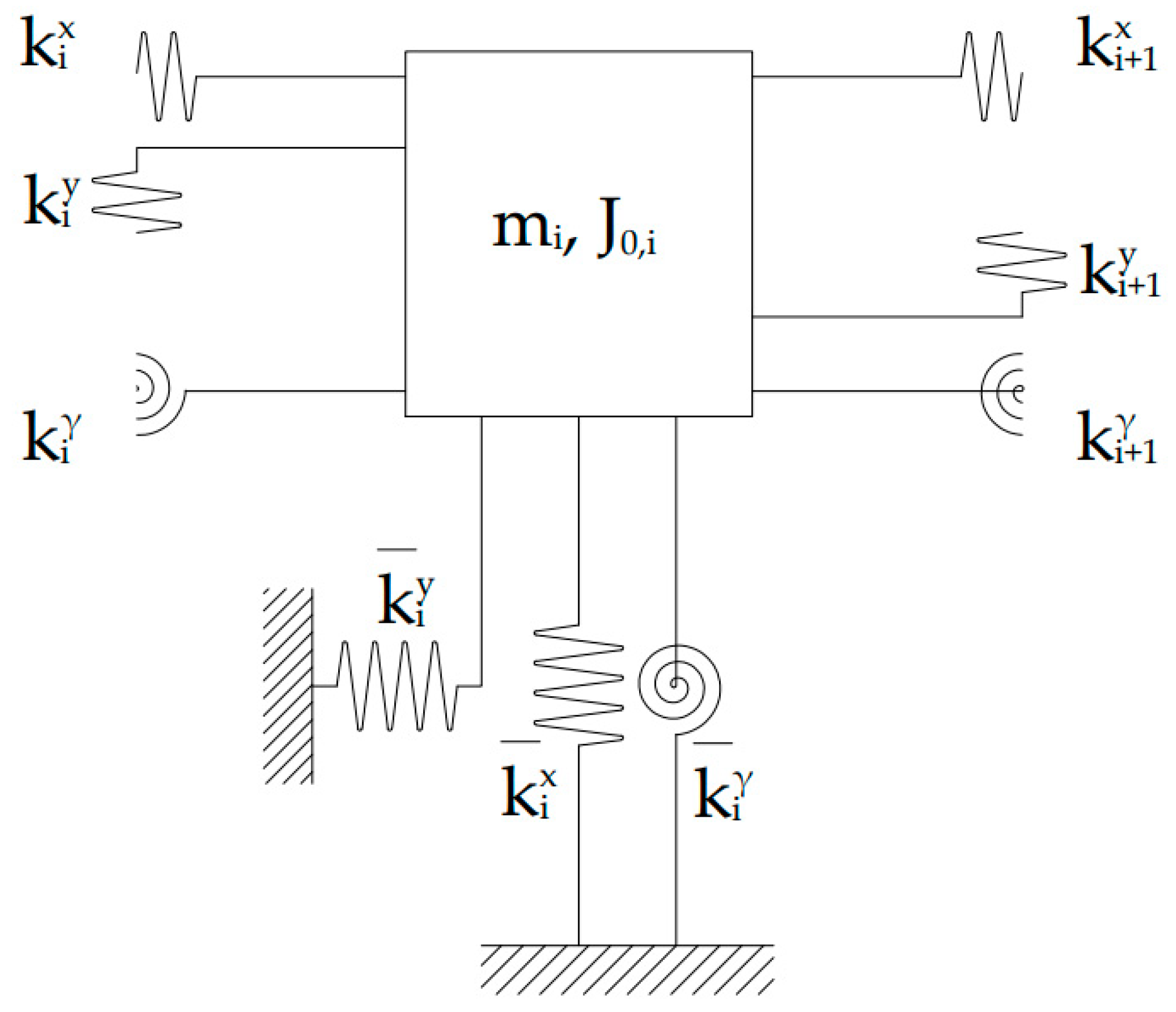
For simplicity, diaphragms are assumed to have only three degrees of freedom, namely two in-plane translations, along x- and y-directions, and the rotation around the z-direction.
Referring to the i-th diaphragm, one can define as the mass, as the polar moment of inertia and and as static moments, and as, respectively, the translational stiffnesses in the x-direction and in the y-direction, as the torsional stiffness, and mixed stiffness terms that regulate the coupling between the translational and rotational degree of freedom, and , and as the displacements in the x-direction, in the y-direction, and the rotation, respectively.
In free undamped vibration conditions, the dynamic equilibrium of the i-th diaphragm, if connected only to the ground, writes:
Now assume that the generic i-th diaphragm is part of a system of n interacting diaphragms. The interaction is assumed to be chain-like, i.e., only between adjacent diaphragms, and it is described by means of linear springs.
In analogy with Equation (1), it is possible to define the mass matrices of the system and , the matrix of polar moments of inertia and the matrices of the static moments and , as well as the stiffness matrices along the three directions , and , and the mixed terms stiffness matrices and , so that the equilibrium equation in compact form writes in terms of 3n × 3n matrices:
Defining then the translational stiffness of the springs connecting the i-th diaphragm with two adjacent diaphragms in the x-direction as and , the stiffness matrix along the x-direction writes:
Similarly to Equation (3), also the stiffness matrix along the y-direction, , and rotation γ, , can be formulated.
The interaction between the i-th diaphragm and the adjacent ones by means of linear springs is described in Figure 1.
3. Numerical Benchmark: System with Three Interacting Diaphragms
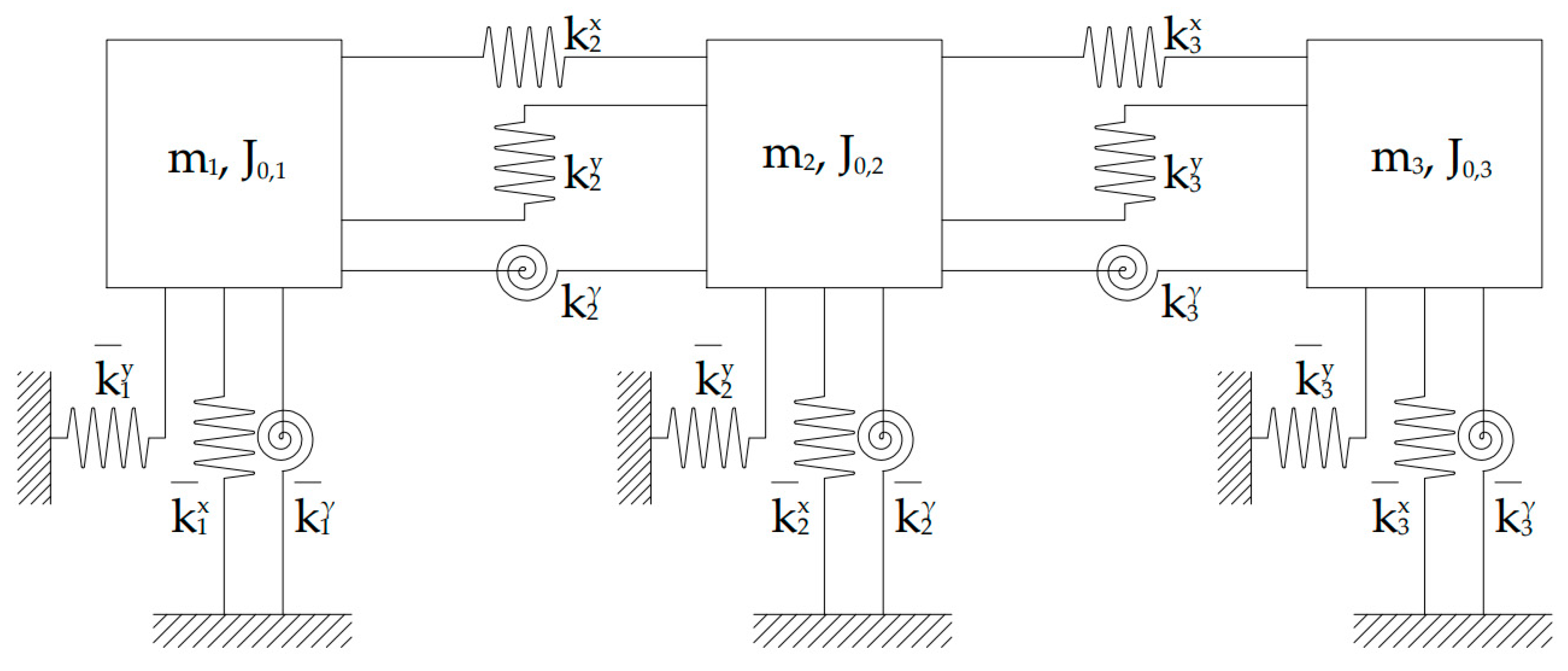
The lumped mass model of three adjacent interacting diaphragms represented in Figure 2 is now considered. The system, presenting a diaphragmatic behavior with a chain-like interaction, is composed of three masses , and , and their respective polar moments of inertia , and .
The values of the translational stiffnesses along the x-direction, , and , the translational stiffnesses along the y-direction, , and , the torsional stiffnesses , and around γ, were chosen to represent typical values of square concrete diaphragms of 50 m on each side. The mixed terms of stiffnesses , , and , , , and the static moments , , and , , have been calculated accordingly. The numerical values of masses, polar moments of inertia, static moments, and stiffnesses are reported in Table 1.
The stiffnesses describing the interaction , , , and , , are set as a fraction (factor varying between 0 and 2), defined as , of the values reported in Table 1, which corresponds to the continuity of the spring. The eigenvalue problem of the above-mentioned system has been then solved to extract the modal parameters, i.e., natural frequencies and mode shapes of the system.
Parametric simulations were conducted to study the relative variation of the modal frequencies of the system with respect to . A simultaneous uniform variation of , , , and , , has been considered. To this aim, the modal frequencies of the system, generally called (with r varying from 1 to 9), were normalized with respect to the fundamental frequency.
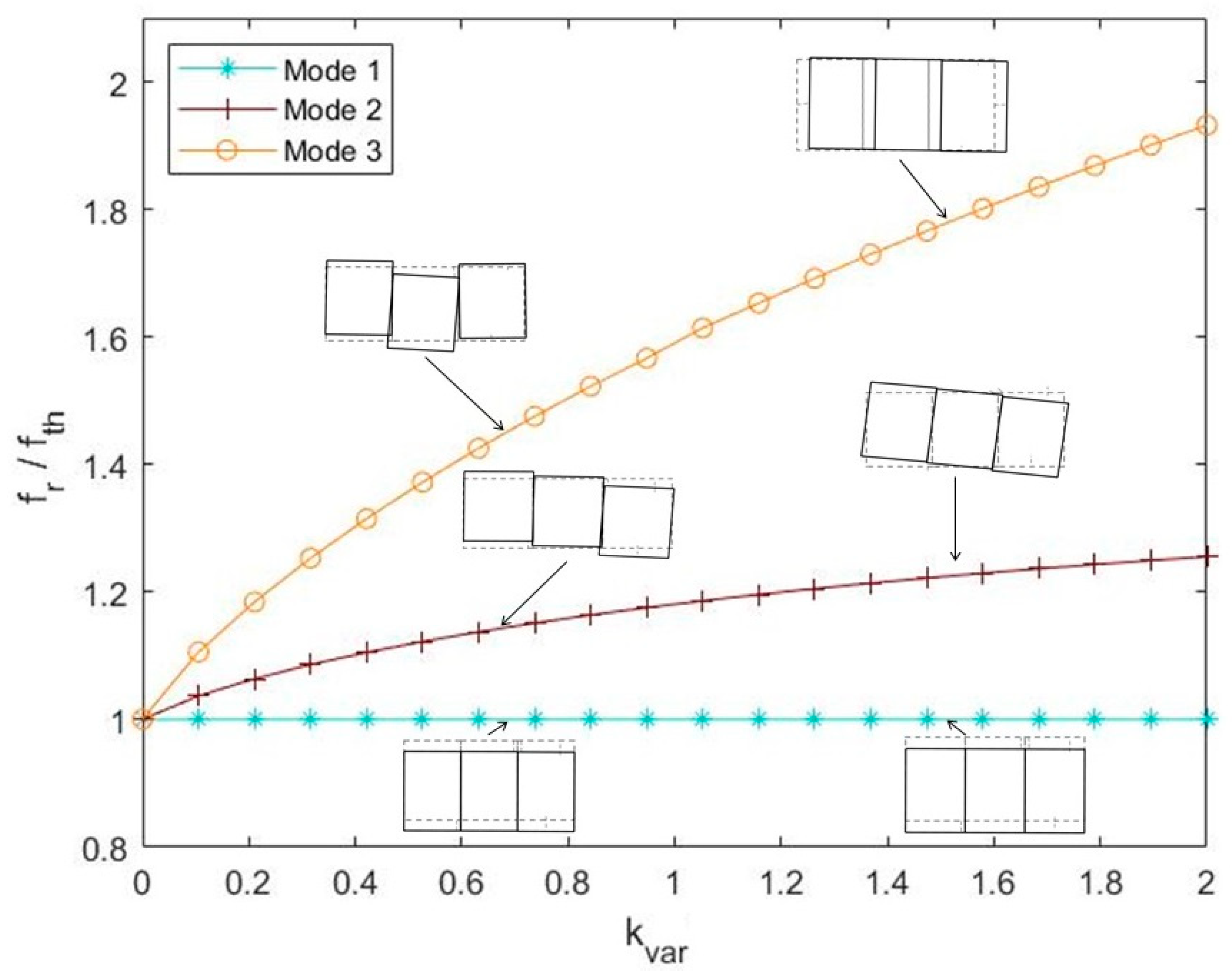
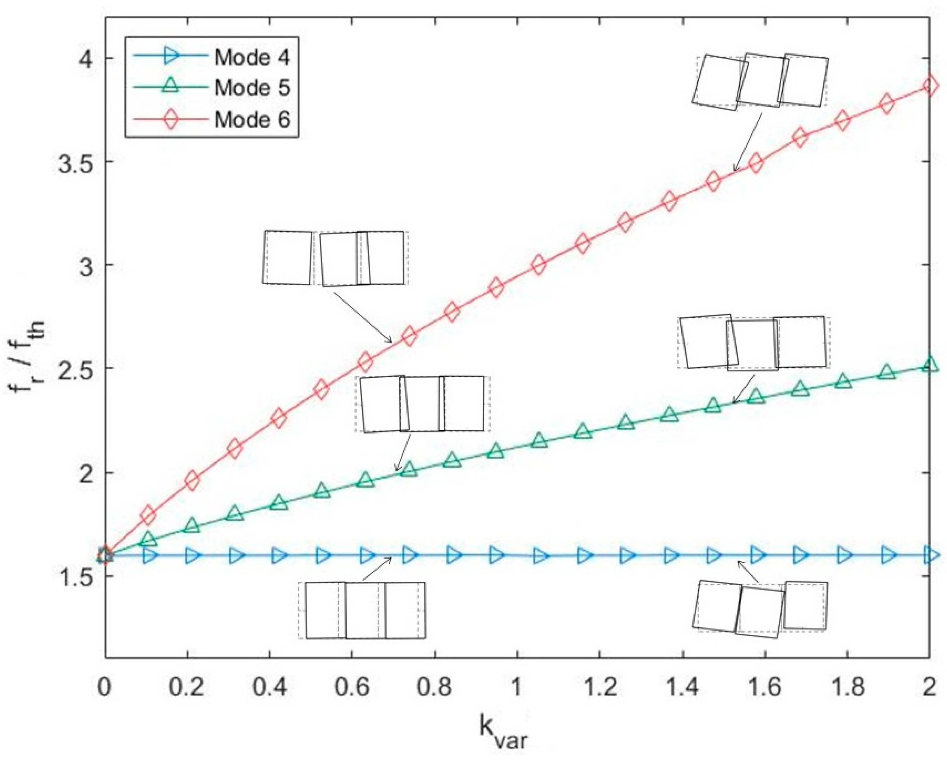
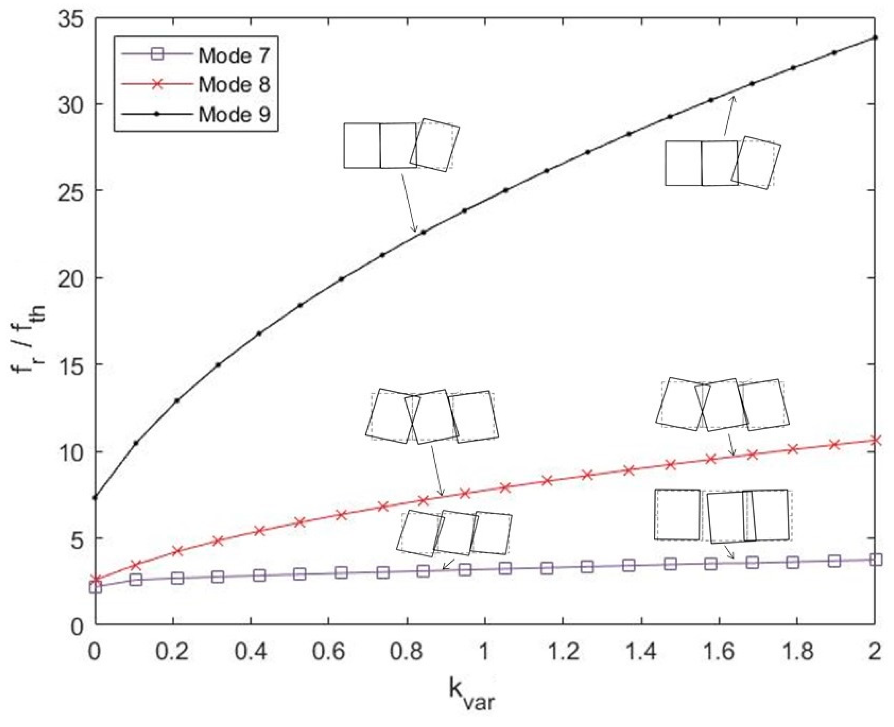
Figure 3, Figure 4 and Figure 5 represent the variation of the 9 modes and of the 9 natural frequencies of the system with respect to . To have a better visualization, the representation is divided into groups of 3 modes each: Figure 3 represents the modes from 1 to 3, Figure 4 from 4 to 6, and Figure 5 from 7 to 9. It is worth noting that the y-axis scales of Figure 3, Figure 4 and Figure 5 are different.
Considerations can be made concerning the modal parameters of the system. In general, an increasing linear trend can be observed in the case of the natural frequencies. Figure 3 shows that the curve corresponding to the first natural frequency is almost flat, while a clear variation of can be observed for the curves corresponding to the second and the third ones ( and ). A similar trend is observed for the other two groups reported in Figure 4 and Figure 5. Therefore, it can be said that increasing values of the stiffness characterizing the interaction clearly affect the higher modal frequencies of each group more. Comparing the three figures, it is noticeable that in the case of the groups of frequencies , , and , , , for values of equal to 0, the numerical value of the frequencies is almost the same. The same behavior is not found for the group of frequencies , and , where the numerical value of is almost double the numerical values of and .
Concerning the mode shapes, when is equal to 0 the diaphragms are uncoupled and show the same three modes. The first mode corresponds to a translational mode along the transversal direction (y-direction) of the system, while the second mode corresponds to a rotational one. While the first mode does not change as a function of , in the case of the second mode, the stiffening effect of the springs characterizing the interaction can be clearly observed: indeed, if the presence of the interaction is clearly visible for values of equal to 0.8, in the case of higher values of the three masses tend to rotate as one single mass, showing therefore a monolithic behavior (see Figure 3).
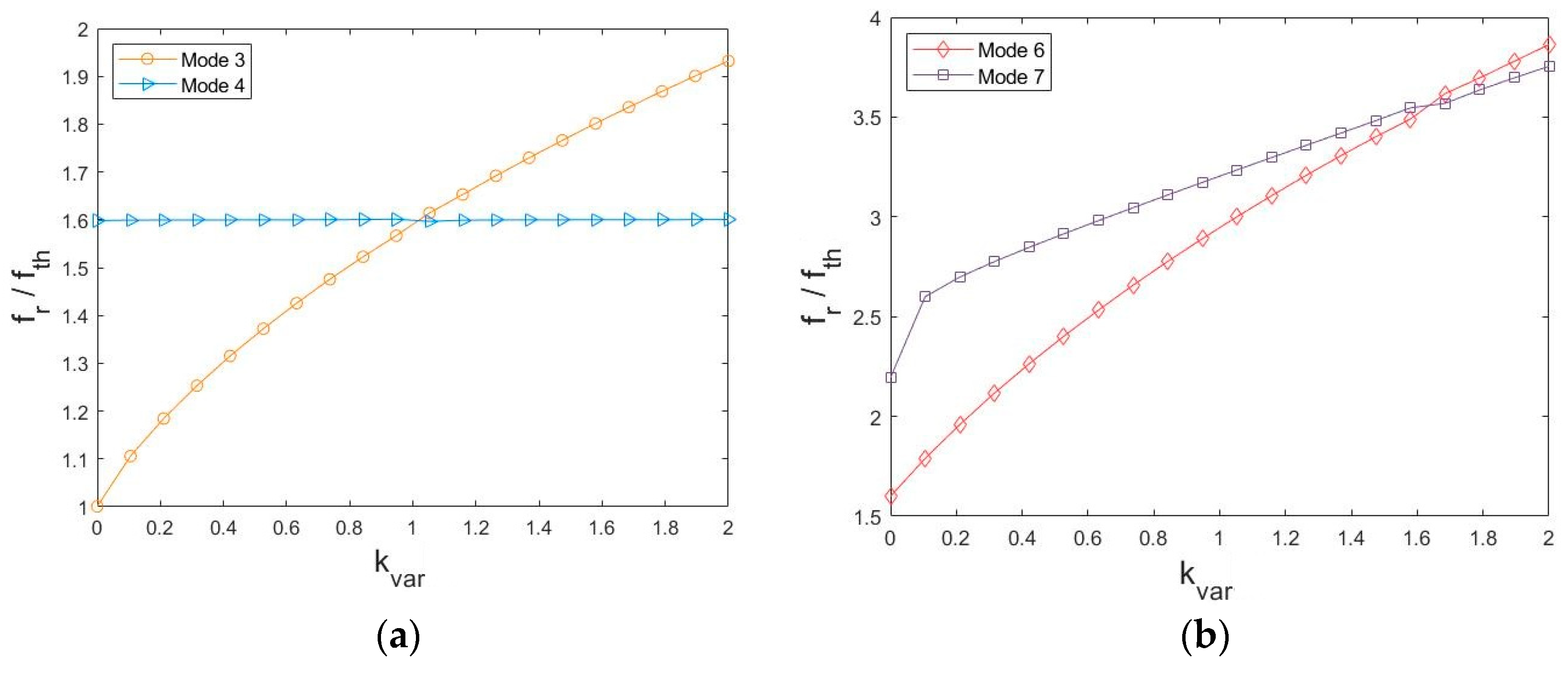
If the frequency curves present a crossing, the modes undergo the so-called re-ordering phenomenon, consisting of a change of order of the modes of the system. In the case of this numerical benchmark, a re-ordering can be observed in two cases, as reported in Figure 6.
A first re-ordering of modes can be observed in correspondence with the third and fourth natural frequencies and of the system for increasing values of (Figure 6a): indeed, in the case of the third one, a translational mode along the longitudinal direction (x-direction) is observed for high values of , instead of a mixed torsional-bending one, observed at low values of (the mode shapes can be found in Figure 3 and Figure 4). A similar situation (Figure 6b) can be observed for the sixth and seventh mode (the mode shapes can be found in Figure 4 and Figure 5).
Consequently, it can be said that for very high values of , i.e., when the three masses behave as one single mass, the first three modes result to be the global modes of the system, corresponding to the translations in the directions x and y and to the rotation. On the other hand, the modes from 4 to 9 can be defined as local modes of the system.
The application of the reported dynamic equation on a numerical benchmark highlights the influence of the interaction between adjacent diaphragms on the dynamic behavior of the system.
4. The Case Study of Morandi’s Hypogeum Pavilion in Turin
Having numerically analyzed the interaction between adjacent diaphragms, which plays a key role in the comprehension of the dynamic behavior of a system, the dynamic model developed in Section 2 can be now exploited in the identification of the modal parameters of a significant case study, represented by Morandi’s Pavilion V of the Turin Exhibition Center. First, a description of the pavilion including some historical background is provided. Then, the experimental setups of a vast dynamic test campaign carried out in 2019 are introduced and described.
4.1. Description of the Pavilion
The Pavilion V, also known as the hypogeum pavilion, was built by Riccardo Morandi in the years 1958–1959 as part of the Turin Exhibition Center. The project was commissioned by Società Torino Esposizioni, almost entirely owned by FIAT motor company, and it was conceived as an extension of the existing Nervi’s halls, mainly aimed at hosting the annual Automobile Show, also considering the upcoming celebrations for the 100th anniversary of Italy’s unification [23].
The pavilion was not only an occasion for Morandi to show his structural art but also an opportunity to exploit the long years of experimentation on prestressed reinforced concrete. The scheme adopted by Morandi for Pavilion V is the so-called balanced beam scheme, widely used by the designer between the 1950s and 1960s, for example in the construction of bridges and overpasses [24]. In particular, Morandi used a version of the balanced beam with subtended tie rods as the main resistant element.
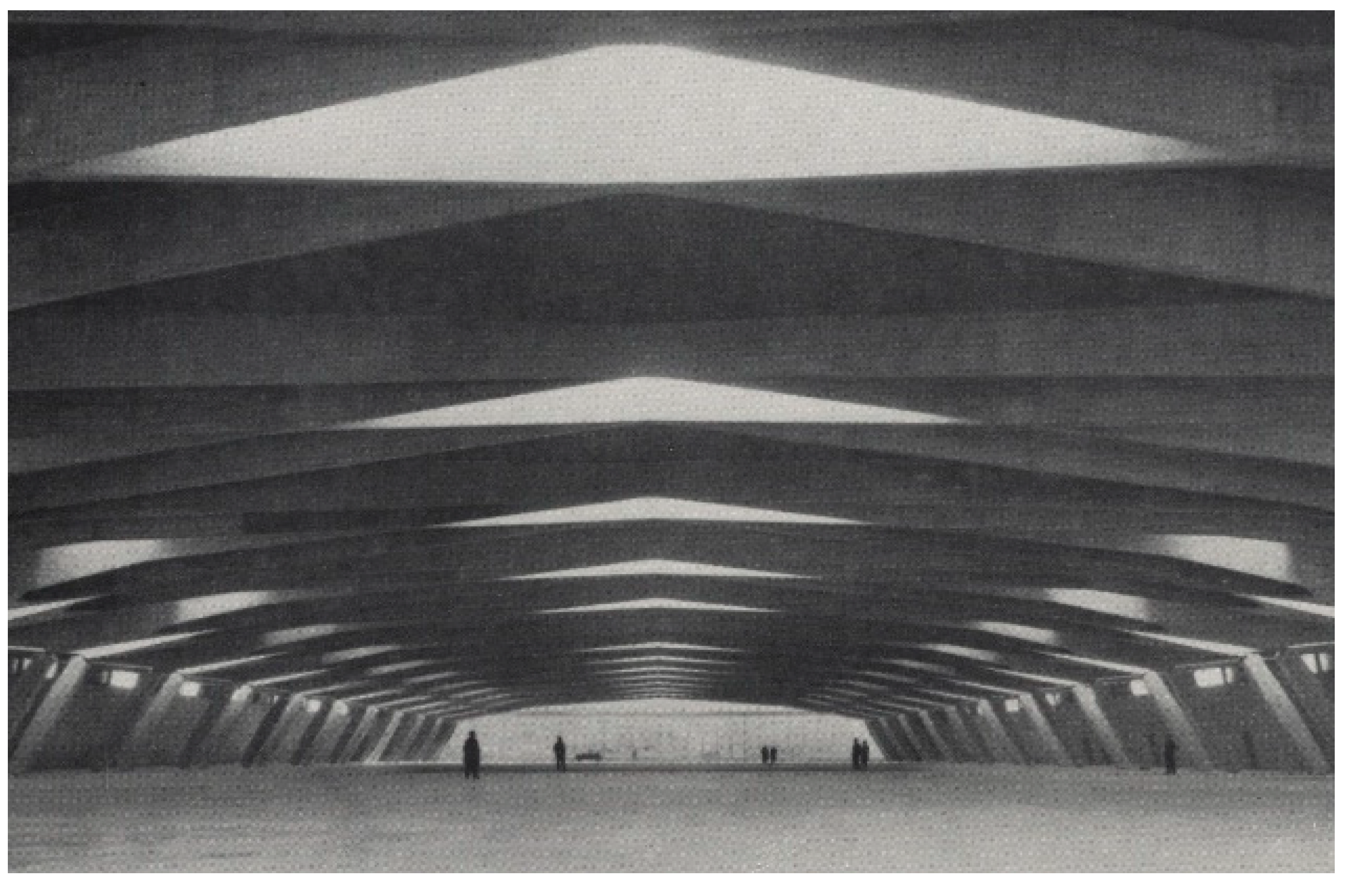
The pavilion is composed of a single large hall with a width of 69 m and a length of 151 m positioned 8 m below the middle level of the surrounding streets. A general view of the pavilion is reported in Figure 7.
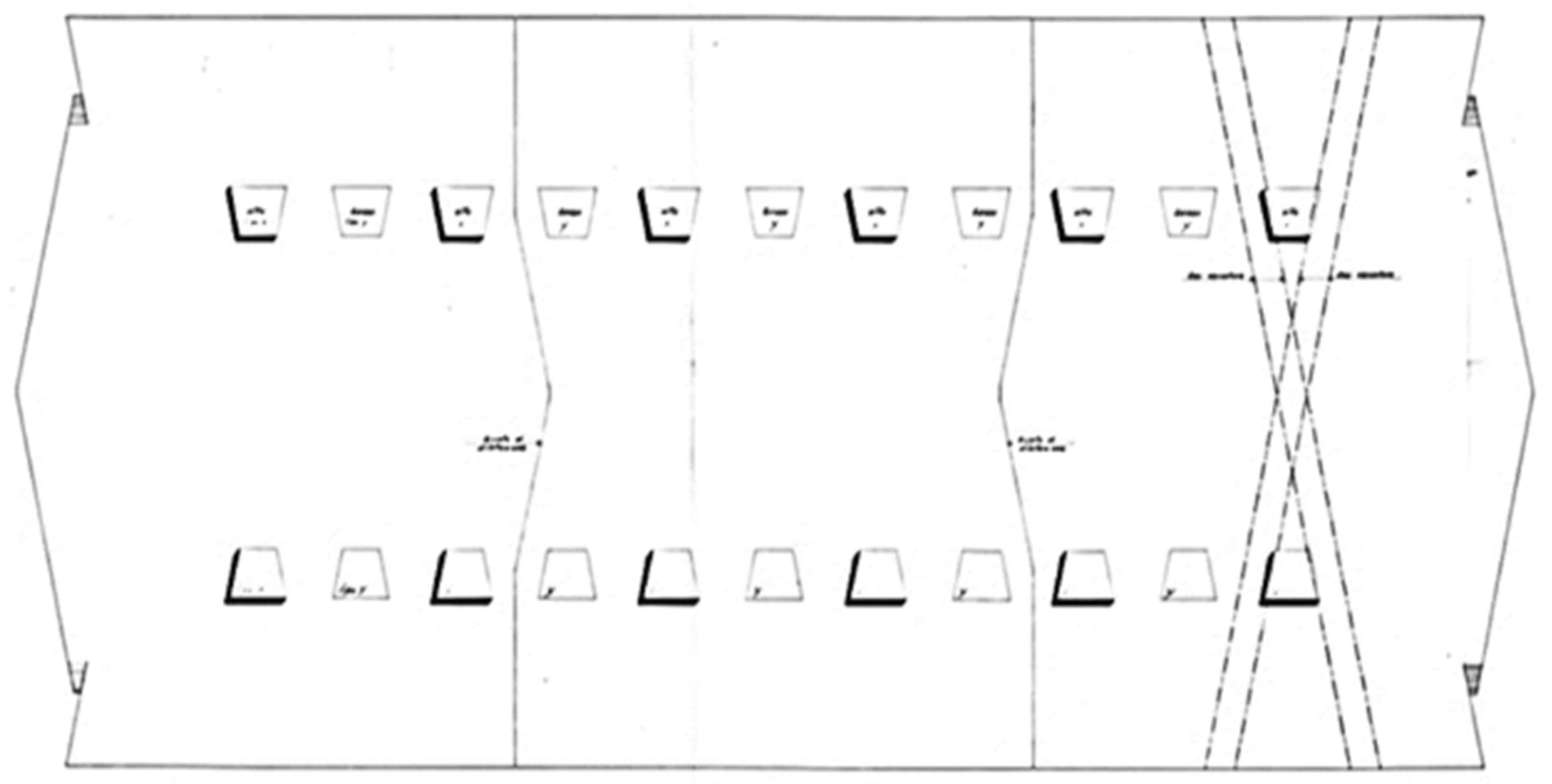
The structure is composed of three blocks linked by two expansion joints, crossing the roof and the external walls. The division of the underground structure into three blocks is clearly observable in Figure 8.
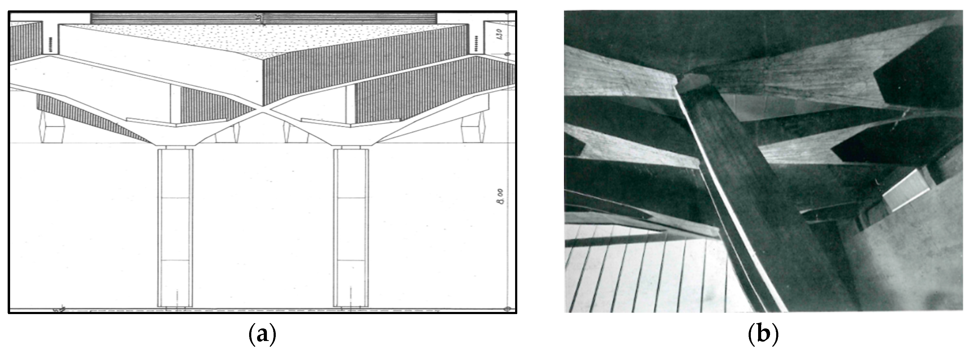
A system of intertwining thin beams in prestressed reinforced concrete composes the roof slab, defining the pavilion’s space. The roof is composed of hollow core concrete and supported by 3.2 m spaced main ribs in prestressed concrete, resting on the pairs of inclined intermediate struts and anchored to the perimeter walls by small strut beams 1 m tall, 50 cm wide, and of variable section. Inside the small rods, the vertical prestressing cables are placed, with the aim to reduce the moment stress arising in the span of the ribs. The bending stresses in the roof and in the crossed ribs are reduced by the inclination of the struts. The balance constraint is produced by the perimeter walls that contain the ground, as well as support the roofing system. The thin ribs would be singularly unstable, but their intertwining makes the structure mostly rigid and robust. One of the intersections is in correspondence with the inclined struts, creating a dovetail geometry [25], as shown in Figure 9.
4.2. Dynamic Test Campaign
A vast test campaign was conducted in February 2019, as reported in [25]. Indeed, non-invasive tests represent an efficient tool to investigate dynamic properties not only for modern civil structures [26] but also for heritage buildings [27]. Among other tests, dynamic acquisitions were carried out employing 20 monoaxial piezoelectric accelerometers, positioned on the ribs and struts. In greater detail, the acquisition system was composed of 20 PCB piezoelectric monoaxial capacitive accelerometers with a sensitivity of 1 V/g, a measurement range between 0 and 3 g, and a resolution of 30μg, whose mass is 17.5 g. The accelerometers were connected via coaxial cables to an acquirer that amplifies the signals, then the signals are sent to a laptop on which the acquisition software was installed. With the intention of favoring modal decoupling, the design of two setups was carried out, based on a preliminary FE model. The first setup allowed to acquire information mainly on the horizontal direction. In fact, the structure exhibits horizontal components of the three diaphragmatic blocks, possibly interacting at their joints, and fixed at the vertical members (longer and shorter strut beams), that define the translational and rotational stiffnesses. The boundary conditions are very clear, in which they reflect the balanced beam conceived by Morandi (see the restraints in Figure 9). A second setup focused instead on the vertical dynamic behavior, which is not accounted for by the model described in Section 2.
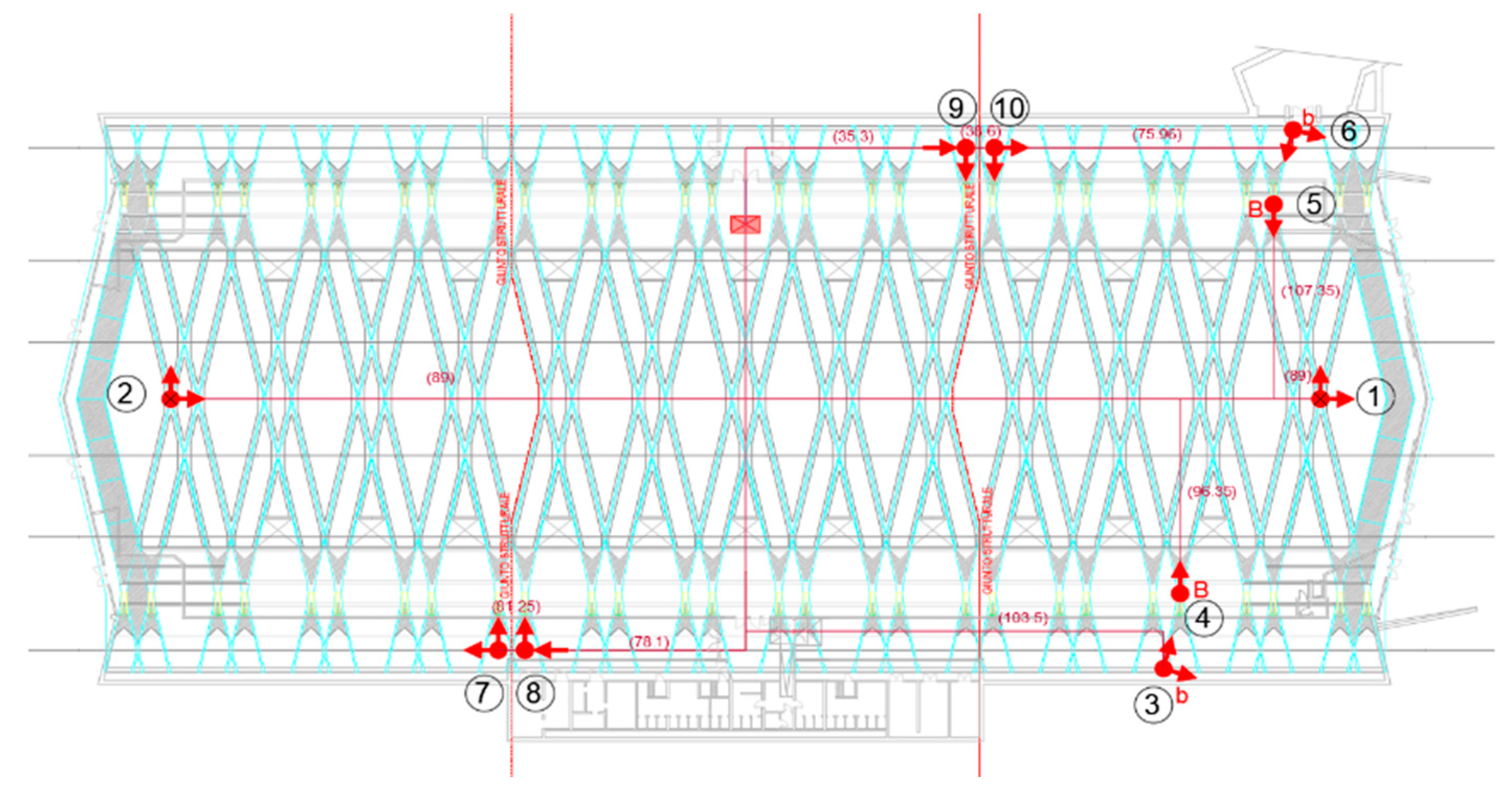
Among the 20 accelerometers used, 8 were positioned in the x-direction, 10 in the y-direction, and 2 in the vertical direction. Only the sensors measuring horizontal components are reported in Figure 10 with red arrows.
The positioning of sensors was designed to study both the global and the local behavior of the structure. In particular, accelerometers 1 and 2 were positioned on the main ribs composing the roof, while accelerometers 4 and 5 were positioned on the large struts. Accelerometers 3 and 6 were positioned on the small struts.
Accelerometers with positions 7, 8, 9, and 10 were placed in correspondence with the joints linking the blocks, to investigate how the interaction affects the dynamic horizontal behavior of the three distinct bodies.
Only ambient excitation signals were used, with acquisitions length between 18 and 98 min and two different sampling frequencies (128 Hz and 256 Hz).
5. Dynamic Identification
5.1. System Identification Procedure
In the case of Pavilion V, the system identification was carried out with algorithm 3 of [28], belonging to the Stochastic Subspace Identification (SSI) family. The aim of this procedure was to understand the horizontal dynamic behavior of the structures, potentially ascribed to dynamic interactions at the joints.
The identification process resulted in the typical stabilization and clustering diagrams [29]. The assumed weighting scheme was that of the classical Canonical Variate Analysis (CVA, SSI-CVA). For the clustering analysis, the Agglomerative Hierarchical cluster method described in [29] has been adopted. The average criterion was then used to identify the cluster reference points, focusing on a bandwidth of the spectrum limited in the 0.5–25 Hz range, in accordance with the preliminary data cleansing.
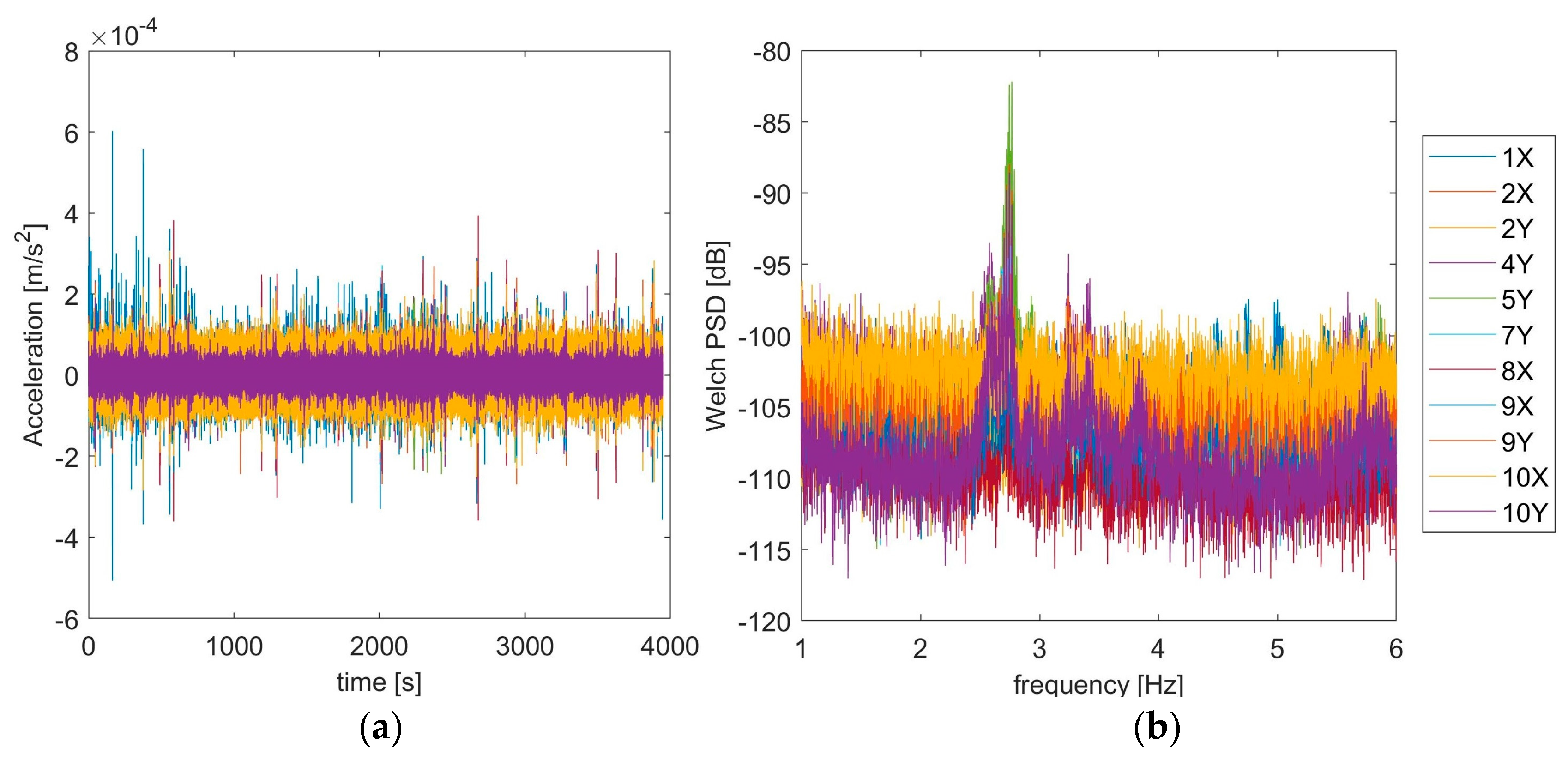
The data were sampled at 256 Hz, in accordance with typical values used for civil structures. The retained signals (horizontal) were detrended and filtered with a band-pass Butterworth filter between 0.5 and 25 Hz with order 5. The signal length is about 64 min; thus, identification sessions were performed on both the entire signal and 8 sessions of 8 min each.
The measured acceleration responses and their Power Spectral Density (PSD) estimate are reported in Figure 11.
5.2. Identified Modes
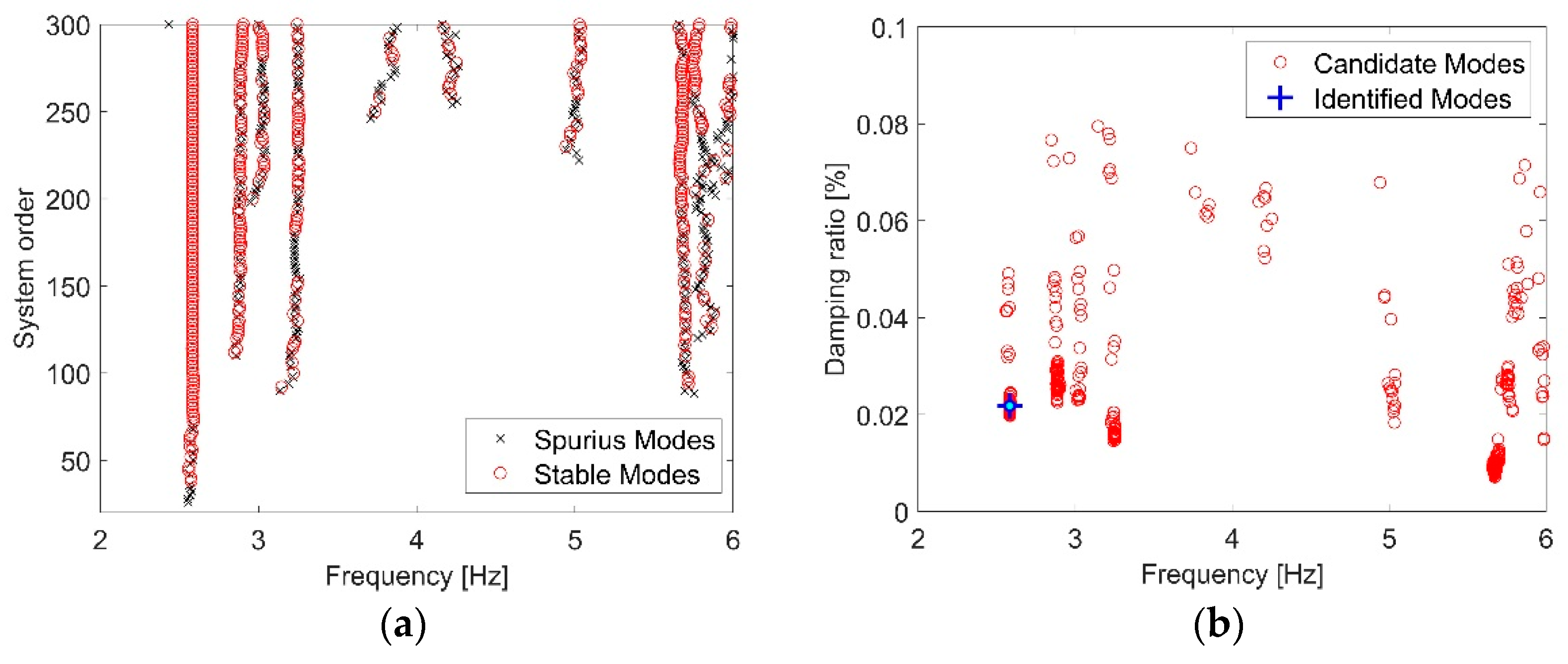
The most recurrent experimental mode was seen to be the one at 2.57 Hz. By way of example, the stabilization and clustering diagrams of the identification of a sub-signal are reported in Figure 12.
The main identified modes are reported in Table 2 in terms of natural frequency and damping ratio. From Figure 12, it can be observed that several clusters are likely to indicate authentic modes. For instance, additional modes are detectable at 3.24 Hz and 5.67 Hz. However, it is worth pointing out that the results presented in this work descend from the assumption that the three blocks belong to the same dynamic system, and a safe attribution, in the presence of a limited number of sensors, will require an accurate mechanical FE model to be calibrated. Due to the redundancy of the measured degrees of freedom with respect to the ones of the diaphragmatic model, the representation of the modal shapes would require an optimization problem to be solved, as reported in Section 6 for the first horizontal mode.
6. Interpretation of the Results and Discussion
For a hypogeum pavilion, vertical modes are relatively more amplified than horizontal ones, especially in the presence of important slab spans. Consequently, the identification of horizontal modes can be affected by unfavorable levels of signal-to-noise ratio (SNR), with respect to the vertical ones. This resulted from a comparison between the normalized spectral entropy of vertical and horizontal channels data, which indicates how close is a spectrum to the Gaussian noise condition. For further details about the relation between entropy and SNR, one can refer to [30,31]. Furthermore, in Morandi’s pavilion, the roofing system is connected at the extrados by non-structural materials, including waterproofing layers. In particular, while the expansion joints between the blocks measure about 0.04 m, the blocks are connected by a thin concrete screed (approximately 0.05 m tick) to create continuity on the walking surface. It was precisely the uncertainty described above that prompted the authors to aid the identifications with the analytical model reported in Section 2.
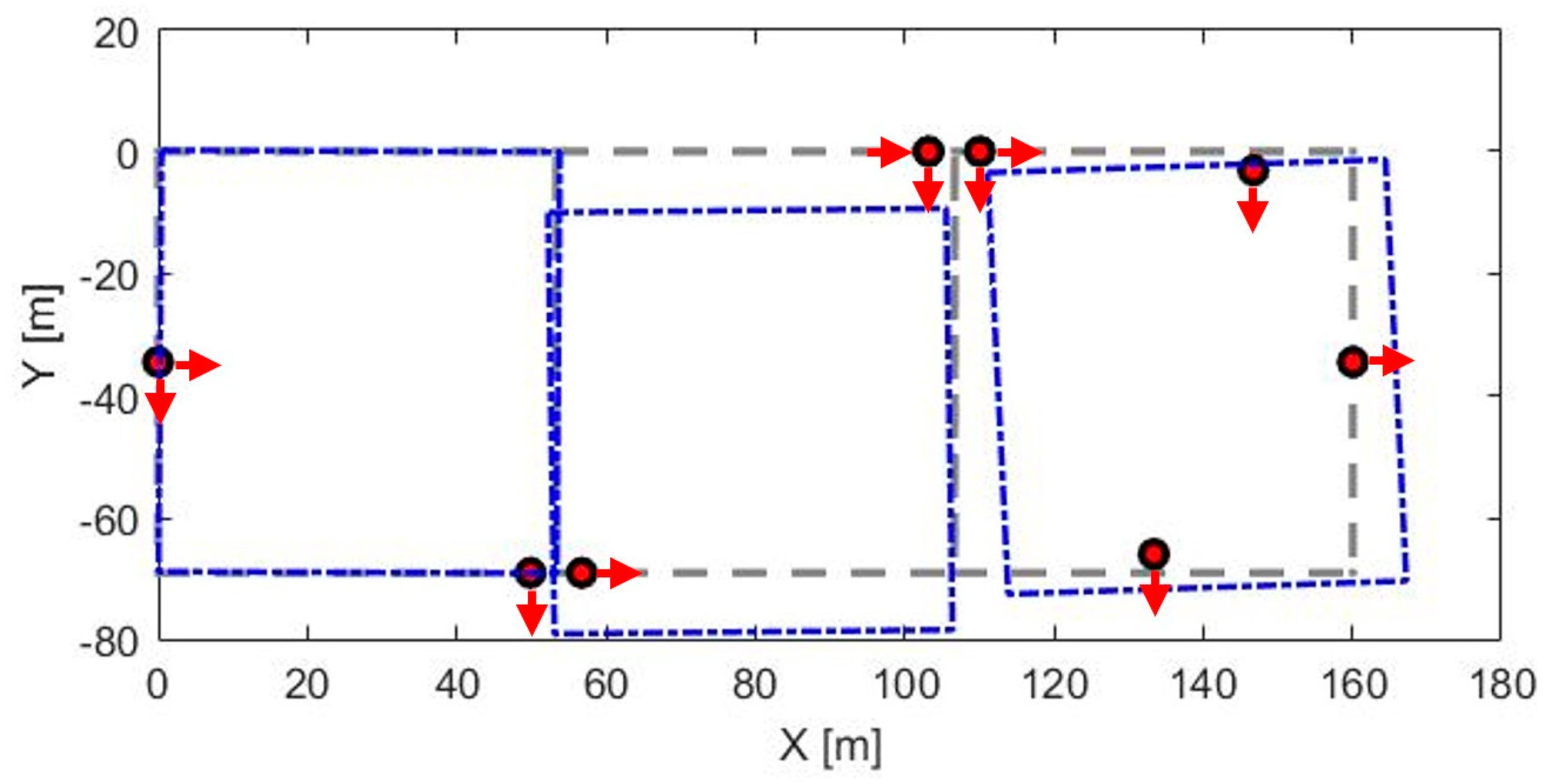
As said before, since the model admits only diaphragmatic degrees of freedom, to compare the experimental results with the model prediction, the horizontal components of the first horizontal mode (identified at 2.57 Hz) have been estimated with the least squares method, also to reduce spillover effects. If denotes the identified eigenvector matrix, the equivalent diaphragmatic body mode components of the eigenvectors can be estimated with a linear transformation matrix D as , where contains the diaphragmatic components, i.e., the two horizontal translations and the rotation about the vertical axis of each block, and is the linear transformation matrix. In accordance with the theoretical model of Section 2, Figure 13 limits the representation to the horizontal components of the examined mode (undeformed configuration in dashed lines, with sensor positions).
From a preliminary analysis of the first mode, the blocks are not appreciably affected by mutual interaction, this being indicative of the full effectiveness of the joints. In other words, the three blocks are likely to behave as fairly separated dynamic systems. This observation can be extended also to joints with relatively low nominal stiffnesses (see Figure 3, Figure 4 and Figure 5). On the other hand, this uncoupled behavior is reflected in Figure 13.
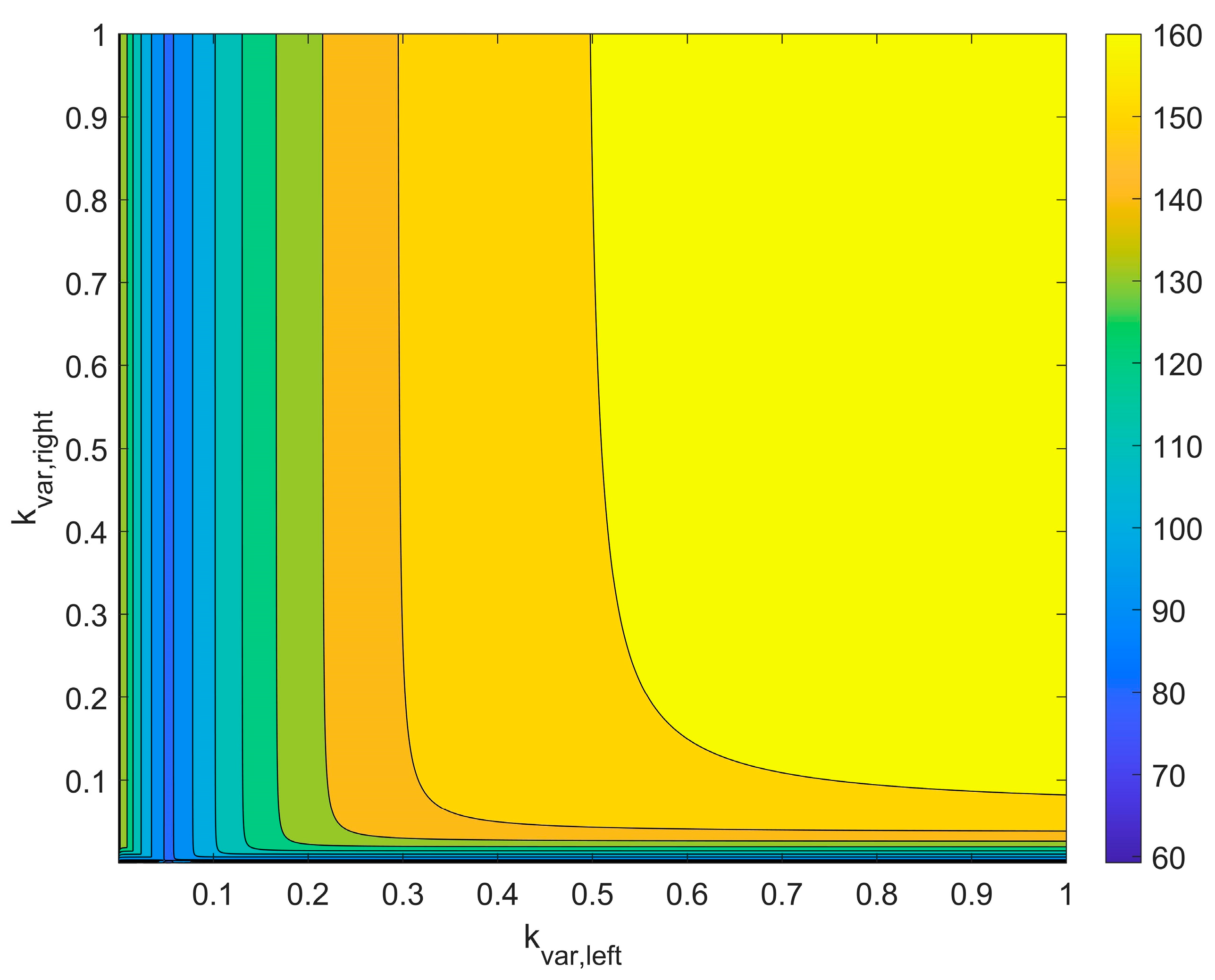
To shed light on the effectiveness of the joints, a numerical analysis was carried out on the nominal values of the model stiffnesses of the joints. The multiplier of the three stiffness components of each joint was varied between 0 and 1. In particular, with reference to Figure 10, two multipliers have been defined as and , respectively. The Modal Assurance Criterion (MAC) [32] between the identified mode shape and the predicted ones was then calculated for each combination of the two multipliers. Defining as the double of the number of modes, the objective function writes [33,34]:
where, for each j-th combination of the two multipliers, and are the weights of the residuals in frequency and mode shapes, respectively, is the j-th identified natural frequency, is the j-th predicted natural frequency, and is the j-th MAC between the identified mode shape and the j-th predicted mode shape.
Figure 14 reports the resulting plot of the objective function, with the assumption to consider only the first vibration mode.
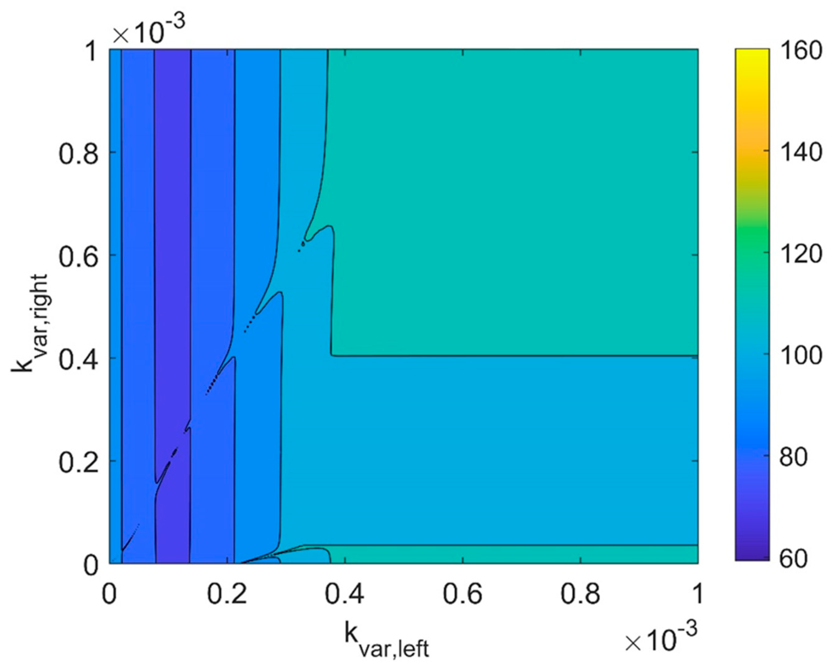
It can be observed from Figure 14 that the objective function tends to decrease dramatically for very low values of and , corresponding to full effectiveness of all the joints. A local minimum is also visible, which is associated with the frequency residual only. Therefore, a further investigation has been conducted for the values of and varying between 0 and 1 × 10⁻³. The results obtained for very low values of the joint stiffnesses are reported in Figure 15, showing that the absolute minimum happens when the joints are fully effective.
The above-described analyses also highlighted a high sensitivity of the joint stiffnesses for values of and close to zero.
7. Conclusions
The dynamics of many civil engineering structures, e.g., multi-span bridges and buildings with interacting bodies, are influenced by the presence of joints, this introducing complexity in the modal response. In particular, uncertainties related to the possible degradation of materials as well as in boundary conditions make it difficult to infer the modal parameters. Consequently, modal identification, even if conducted in the linear field, can become a difficult task, calling for simplified models to unravel different components and aid the mode attribution process.
Morandi’s Pavilion V of the Turin Exhibition Center is an example of a building with interacting bodies, thus reflecting all the previously stated criticalities. A further problem of this structure is related to its underground configuration, which results in low SNR unfavorably affecting the operational modal analysis.
From the results of this work, the following general conclusions can be drawn:
- Not only the presence of joints does result in modal complexity, but also in very high sensitivity of the stiffness parameters, especially when the joints are fully effective.
- This complexity also affects the design of the experimental setups, which often are not able to capture the whole-body dynamics.
Possible development of the analysis will contemplate the identification of the three blocks as independent bodies with the consequent updating of a high-fidelity numerical model. It is worth noting that the results reported in this paper are valid in operational conditions. This means that, in the presence of a strong excitation (e.g., an earthquake), the stiffness of the joints could be activated in the non-linear field, giving rise to even more complex behavior.
Author Contributions
Conceptualization, R.C., L.S., V.O., E.L. and G.M.; methodology, R.C., L.S., V.O., E.L. and G.M.; software, L.S. and G.M.; validation, R.C., L.S., E.L., V.O. and G.M.; formal analysis, L.S. and G.M.; investigation, R.C., L.S., V.O., E.L. and G.M.; resources, R.C., L.S., V.O., E.L. and G.M.; data curation, R.C., L.S., V.O., E.L. and G.M.; writing—original draft preparation, L.S. and V.O.; writing—review and editing, R.C., E.L. and G.M.; visualization, R.C., L.S., V.O., E.L. and G.M.; supervision, R.C., E.L., and G.M.; project administration, R.C.; funding acquisition, R.C. and E.L. All authors have read and agreed to the published version of the manuscript.
Funding
This research received no external funding.
Institutional Review Board Statement
Not applicable.
Informed Consent Statement
Not applicable.
Data Availability Statement
Not applicable.
Conflicts of Interest
The authors declare no conflict of interest.
References
- Reynders, E. System identification methods for (operational) modal analysis: Review and comparison. Arch. Comput. Methods Eng. 2012, 19, 51–124. [Google Scholar] [CrossRef]
- Brincker, R.; Ventura, C.; Andersen, P. Why output-only modal testing is a desirable tool for a wide range of practical applications. In Proceedings of the International Modal Analysis Conference (IMAC) XXI, Kissimmee, FL, USA, 3–6 February 2003; Volume 265. [Google Scholar]
- Ren, W.-X.; Zong, Z.-H. Output-only modal parameter identification of civil engineering structures. Struct. Eng. Mech. 2004, 17, 429–444. [Google Scholar] [CrossRef] [Green Version]
- Ceravolo, R.; Abbiati, G. Time domain identification of structures: Comparative analysis of output-only methods. J. Eng. Mech. 2013, 139, 537–544. [Google Scholar] [CrossRef]
- Andersen, P.; Brincker, R.; Peeters, B.; De Roeck, G.; Hermans, L.; Krämer, C. Comparison of system identification methods using ambient bridge test data. In Proceedings of the 17th International Modal Analysis Conference (IMAC), Kissimmee, FL, USA, 8–11 February 1999; pp. 1035–1041. [Google Scholar]
- Peeters, B. System Identification and Damage Detection in Civil Engeneering. Ph.D. Thesis, Katholieke Universiteit Leuven, Leuven, Belgium, 2000. [Google Scholar]
- Peeters, B.; De Roeck, G. Stochastic system identification for operational modal analysis: A review. J. Dyn. Syst. Meas. Control 2001, 123, 659–667. [Google Scholar] [CrossRef]
- Reynders, E.; Pintelon, R.; De Roeck, G. Uncertainty bounds on modal parameters obtained from stochastic subspace identification. Mech. Syst. Signal Process. 2008, 22, 948–969. [Google Scholar] [CrossRef]
- Van Overschee, P.; De Moor, B.L. Subspace Identification for Linear Systems: Theory—Implementation—Applications; Springer Science & Business Media: Berlin/Heidelberg, Germany, 2012. [Google Scholar]
- Peeters, B.; De Roeck, G. Reference-based stochastic subspace identification for output-only modal analysis. Mech. Syst. Signal Process. 1999, 13, 855–878. [Google Scholar] [CrossRef] [Green Version]
- Brincker, R.; Andersen, P. Understanding stochastic subspace identification. In Proceedings of the Conference and Exposition on Structural Dynamics IMAC-XXIV, St. Louis, MO, USA, 30 January–2 February 2006. [Google Scholar]
- Kim, J.; Lynch, J.P. Subspace system identification of support-excited structures—Part I: Theory and black-box system identification. Earthq. Eng. Struct. Dyn. 2012, 41, 2235–2251. [Google Scholar] [CrossRef] [Green Version]
- Ubertini, F.; Gentile, C.; Materazzi, A.L. Automated modal identification in operational conditions and its application to bridges. Eng. Struct. 2013, 46, 264–278. [Google Scholar] [CrossRef]
- Bonato, P.; Ceravolo, R.; De Stefano, A.; Molinari, F. Cross-time frequency techniques for the identification of masonry buildings. Mech. Syst. Signal Process. 2000, 14, 91–109. [Google Scholar] [CrossRef]
- Peeters, B.; De Roeck, G.; Pollet, T.; Schueremans, L. Stochastic subspace techniques applied to parameter identification of civil engineering structures. New Adv. Modal Synth. Large Struct. 1997, 145–156. [Google Scholar]
- Londono, N.A.; Desjardins, S.L.; Lau, D.T. Use of stochastic subspace identification methods for post-disaster condition assessment of highway bridges. In Proceedings of the 13th World Conference on Earthquake Engineering, Vancouver, BC, Canada, 1–6 August 2004. [Google Scholar]
- Ljung, L. Black-box models from input-output measurements. In Proceedings of the (IMTC 2001) 18th IEEE Instrumentation and Measurement Technology Conference, Rediscovering Measurement in the Age of Informatics (Cat. No. 01CH 37188), Budapest, Hungary, 21–23 May 2001; Volume 1, pp. 138–146. [Google Scholar]
- Sjöberg, J.; Zhang, Q.; Ljung, L.; Benveniste, A.; Delyon, B.; Glorennec, P.-Y.; Hjalmarsson, H.; Juditsky, A. Nonlinear black-box modeling in system identification: A unified overview. Automatica 1995, 31, 1691–1724. [Google Scholar] [CrossRef] [Green Version]
- Alvin, K.F.; Robertson, A.N.; Reich, G.W.; Park, K.C. Structural system identification: From reality to models. Comput. Struct. 2003, 81, 1149–1176. [Google Scholar] [CrossRef]
- Berman, A.; Nagy, E.J. Improvement of a large analytical model using test data. AIAA J. 1983, 21, 1168–1173. [Google Scholar] [CrossRef]
- Sobester, A.; Forrester, A.; Keane, A. Engineering Design via Surrogate Modelling: A Practical Guide; John Wiley & Sons: Hoboken, NJ, USA, 2008. [Google Scholar]
- Qin, S.; Zhang, Y.; Zhou, Y.-L.; Kang, J. Dynamic model updating for bridge structures using the kriging model and PSO algorithm ensemble with higher vibration modes. Sensors 2018, 18, 1879. [Google Scholar] [CrossRef] [Green Version]
- Bruno, E. Riccardo Morandi per il Vpadiglione di Torino Esposizioni. In La Concezione Strutturale: Architettura e Ingegneria in Italia Negli Anni 50 e 60; P. Desideri, A., Magistris, C., Olmo, M., Pogacnik, S., Sorace, S., Eds.; Umberto Allemandi & C.: Torino, Italy, 2013; pp. 229–238. [Google Scholar]
- Levi, F.; Chiorino, M.A. Concrete in Italy. A review of a century of concrete progress in Italy, Part 1: Technique and architecture. Concr. Int. 2004, 26, 55–61. [Google Scholar]
- Earthquake Engineering & Dynamics Laboratory. Relazione Sulle Prove di Caratterizzazione Dinamica del Padiglione Morandi di Torino Esposizioni; Earthquake Engineering & Dynamics Laboratory: Torino, Italy, 2019. [Google Scholar]
- Pierdicca, A.; Clementi, F.; Fortunati, A.; Lenci, S. Tracking modal parameters evolution of a school building during retrofitting works. Bull. Earthq. Eng. 2019, 17, 1029–1052. [Google Scholar] [CrossRef]
- Giordano, E.; Marcheggiani, L.; Formisano, A.; Clementi, F. Application of a Non-Invasive Technique for the Preservation of a Fortified Masonry Tower. Infrastructures 2022, 7, 30. [Google Scholar] [CrossRef]
- Van Overschee, P.; Moor, B. De Stochastic identification. In Subspace Identification for Linear Systems; Springer: Berlin/Heidelberg, Germany, 1996; pp. 57–93. [Google Scholar]
- Pecorelli, M.L.; Ceravolo, R.; Epicoco, R. An Automatic Modal Identification Procedure for the Permanent Dynamic Monitoring of the Sanctuary of Vicoforte. Int. J. Archit. Herit. 2018, 14, 630–644. [Google Scholar] [CrossRef]
- Freiman, A.; Pinchas, M. A maximum entropy inspired model for the convolutional noise PDF. Digit. Signal Process. 2015, 39, 35–49. [Google Scholar] [CrossRef]
- Beenamol, M.; Prabavathy, S.; Mohanalin, J. Wavelet based seismic signal de-noising using Shannon and Tsallis entropy. Comput. Math. Appl. 2012, 64, 3580–3593. [Google Scholar] [CrossRef] [Green Version]
- Allemang, R.J. The modal assurance criterion—Twenty years of use and abuse. Sound Vib. 2003, 37, 14–23. [Google Scholar]
- Merce, R.N.; Doz, G.N.; de Brito, J.L.V.; Macdonald, J.; Friswell, M.I. Finite element model updating of a suspension bridge using ansys software. In Proceedings of the Inverse Problems, Design and Optimization Symposium, Miami, FL, USA, 16–18 April 2007. [Google Scholar]
- Moller, P.W.; Friberg, O. Updating large finite element models in structural dynamics. AIAA J. 1998, 36, 1861–1868. [Google Scholar] [CrossRef]
Figure 1.
Lumped mass model of the interacting i-th diaphragm.

Figure 2.
Lumped mass model of three adjacent interactive diaphragms.

Figure 3.
Variation of the modes and of the natural frequencies of the system from 1 to 3 as a function of .
Figure 3.
Variation of the modes and of the natural frequencies of the system from 1 to 3 as a function of .

Figure 4.
Variation of the modes and of the natural frequencies of the system from 4 to 6 as a function of .
Figure 4.
Variation of the modes and of the natural frequencies of the system from 4 to 6 as a function of .

Figure 5.
Variation of the modes and of the natural frequencies of the system from 7 to 9 as a function of .
Figure 5.
Variation of the modes and of the natural frequencies of the system from 7 to 9 as a function of .

Figure 6.
Re-ordering of modes: (a) modes 3 and 4; (b) modes 6 and 7.

Figure 7.
Interior view of Morandi’s Pavilion V.

Figure 8.
Scheme of the plan of Morandi’s Pavilion V showing the division into three blocks linked by joints.
Figure 8.
Scheme of the plan of Morandi’s Pavilion V showing the division into three blocks linked by joints.

Figure 9.
Intersection of the thin ribs creating a dovetail geometry: (a) general section; (b) detail of the restraints of the shorter strut beams.
Figure 9.
Intersection of the thin ribs creating a dovetail geometry: (a) general section; (b) detail of the restraints of the shorter strut beams.

Figure 10.
Sensors on the x-y plane in Setup 1. The numbers 1–10 in figure refer to identifiers of different sensors position.
Figure 10.
Sensors on the x-y plane in Setup 1. The numbers 1–10 in figure refer to identifiers of different sensors position.

Figure 11.
Measured acceleration responses: (a) time−domain; (b) frequency−domain.

Figure 12.
Stabilization (a) and clustering (b) diagram of the identification performed on the sixth sub−signal of setup 1 of the entire Pavilion V, with evidence of the mode at 2.57 Hz.
Figure 12.
Stabilization (a) and clustering (b) diagram of the identification performed on the sixth sub−signal of setup 1 of the entire Pavilion V, with evidence of the mode at 2.57 Hz.

Figure 13.
Identified mode shape #1 at 2.57 Hz (horizontal components).

Figure 14.
Objective function for a variation of and in the range between 0 and 1.

Figure 15.
Objective function for a variation of and in the range between 0 and 1 × 10⁻³.


Table 1.
Numerical values of parameters.
| Parameter | Numerical Value | Unit |
|---|---|---|
| 4.2 × 10⁶ | kg | |
| 1.0 × 10¹⁰ | N·m2 | |
| 3.2 × 10¹⁰ | N·m2 | |
| 7.5 × 10¹⁰ | N·m2 | |
| 1.1 × 10⁸ | kg·m | |
| 3.2 × 10⁸ | kg·m | |
| 5.4 × 10⁸ | kg·m | |
| −1.5 × 10⁸ | kg·m | |
| 8.7 × 10⁸ | N/m | |
| 3.4 × 10⁸ | N/m | |
| 2.2 × 10¹² | N/m | |
| 3.9 × 10¹² | N/m | |
| 7.4 × 10¹² | N/m | |
| −3.0 × 10¹⁰ | N·m/m | |
| 8.6 × 10⁹ | N·m/m | |
| 2.6 × 10¹⁰ | N·m/m | |
| 4.3 × 10¹⁰ | N·m/m | |
| 8.7 × 10⁸ | N/m | |
| 3.4 × 10⁸ | N/m | |
| 2.2 × 10¹² | N/m |
Table 2.
Identified modes of the entire pavilion.
| Description | Mode Id. | Natural Frequency (Hz) | Damping Ratio (%) |
|---|---|---|---|
| Horizontal (with roof bending) mode | 1 | 2.57 | 2.11 |
| Mainly vertical mode | 2 | 2.73 | 0.91 |
Publisher’s Note: MDPI stays neutral with regard to jurisdictional claims in published maps and institutional affiliations. |
© 2022 by the authors. Licensee MDPI, Basel, Switzerland. This article is an open access article distributed under the terms and conditions of the Creative Commons Attribution (CC BY) license (https://creativecommons.org/licenses/by/4.0/).
Share and Cite
MDPI and ACS Style
Ceravolo, R.; Lenticchia, E.; Miraglia, G.; Oliva, V.; Scussolini, L. Modal Identification of Structures with Interacting Diaphragms. Appl. Sci. 2022, 12, 4030. https://0-doi-org.brum.beds.ac.uk/10.3390/app12084030
AMA Style
Ceravolo R, Lenticchia E, Miraglia G, Oliva V, Scussolini L. Modal Identification of Structures with Interacting Diaphragms. Applied Sciences. 2022; 12(8):4030. https://0-doi-org.brum.beds.ac.uk/10.3390/app12084030
Chicago/Turabian StyleCeravolo, Rosario, Erica Lenticchia, Gaetano Miraglia, Valerio Oliva, and Linda Scussolini. 2022. "Modal Identification of Structures with Interacting Diaphragms" Applied Sciences 12, no. 8: 4030. https://0-doi-org.brum.beds.ac.uk/10.3390/app12084030
Note that from the first issue of 2016, this journal uses article numbers instead of page numbers. See further details here.