
Dynamic Bottleneck Identification of Manufacturing Resources in Complex Manufacturing System

1
School of Mechanical Engineering, Jiangnan University, Wuxi 214122, China
2
Key Laboratory of Advanced Manufacturing Equipment Technology, School of Mechanical Engineering, Jiangnan University, Wuxi 214122, China
*
Author to whom correspondence should be addressed.
Appl. Sci. 2022, 12(9), 4195; https://0-doi-org.brum.beds.ac.uk/10.3390/app12094195
Submission received: 8 March 2022
/
Revised: 15 April 2022
/
Accepted: 18 April 2022
/
Published: 21 April 2022
(This article belongs to the Topic Modern Technologies and Manufacturing Systems)
Abstract
:Bottleneck identification is of great interest in discrete manufacturing fields, as they limit the system’s throughput. However, the bottlenecks are difficult to accurately identify due to the instability and complexity of discrete manufacturing systems. This paper proposes a dynamic bottleneck identification method (DBI-BS) that is based on effective buffers and fine-grained machine states to identify bottlenecks accurately. First, the complex manufacturing system (CMS) with strong coupling between elements is decoupled into several independent parts under the guidance of the effective buffer theory. Then, the machine activity duration method is improved through further fine-grained division, and the machine states are described by the timing flow model. The method to quantify the degree of bottleneck that restricts the system throughput (TH) is proposed on the basis of the turning point theory, and the one-to-one mapping relationship between the simulated and authentic complex manufacturing systems is also studied. Simulation results show that the DBI-BS can effectively identify dynamic bottlenecks in complex manufacturing processes, and the decoupling of complex systems can effectively improve the accuracy of dynamic bottleneck identification.
1. Introduction
The fusion of multiple technologies (manufacturing IoT [1], digital twins [2], big data [3], neural networks [4], etc.) has brought great opportunities and challenges to the transformation of manufacturing [5]. The new industrial revolution, commonly known as Industry 4.0, originated in Germany has arrived [6]. Increasing productivity is one of the explicit goals set forth by Industry 4.0 originated in Germany [7]. In addition, the deteriorating new crown epidemic has dramatically damaged the production capacity of the global manufacturing industry, so there is an urgent need to increase the output of the current manufacturing system. Higher productivity is ranked as the number one technology investment priority for manufacturing companies for the next decade [7].
The change in manufacturing mode and the need to improve manufacturing capabilities have significantly increased the complexity of manufacturing, which has brought considerable challenges to the production management of the workshop [8]. In this situation, the CMS has been widely used in manufacturing enterprises [7]. CMS allows a rapid response to fluctuations inside and outside the workshop and comprehensive utilization of existing manufacturing resources to increase system productivity. A typical CMS is a hybrid process workshop (HFS) consisting of several serial stages with parallel machines. The job must be processed at every stage on one machine.
According to the theory of constraints (TOC) [9], there is a stage that limits the entire production capacity or significantly limits the throughput of the workshop, which is called the bottleneck stage [3]. The bottleneck is defined as the equipment that has the most significant impact on the overall performance of the production system. In the case of limited resources, priority is given to improving the production of bottleneck equipment or allocating resources. For example, defining the maintenance of bottleneck equipment as the highest priority can effectively improve the overall performance of the CMS.
However, there are many challenges in effectively identifying bottlenecks in complex systems. First, the strongly coupled elements of the CMS [10] can increase the difficulty of bottleneck identification. Second, disturbances in the production process lead to a constant drift of bottlenecks [8]. Third, the lack of accurate bottleneck quantification methods makes it difficult to determine the degree of different bottlenecks restricting the system [11]. To deal with the above problems, this paper proposes a simulation and data hybrid-driven method (DBI-BS) to identify the dynamic bottlenecks in CMS. In addition, the DBI-BS method proposed in this paper is verified in a discrete simulation system of authentic CMS processes. The contributions of this paper are summarized as:
- (1)
- The effective buffers are used to decouple CMS to avoid the coupling between the system’s various elements, causing bottleneck misjudgments. The definition and identification method of the effective buffer zone are also given.
- (2)
- The data-driven method is used to identify the dynamic bottleneck, and a data-driven dynamic bottleneck model is established. The equipment operating state is further divided into fine-grained divisions to improve identification accuracy, and it is judged whether the state is effective.
- (3)
- Using the actual production data of the workshop to guide the simulation model, the production logic relationship between the manufacturing entity and the simulation agent is clarified, and the simulation model is closer to the actual production.
The rest of this paper is organized as follows. Section 2 reviews the literature of bottleneck identification. Section 3 introduces the CMS and its decoupling methods, and the proposed dynamic bottleneck identification method (DBI-BS) is also presented in this section. The simulation verifications in AnyLogic using a real discrete manufacturing workshop are conducted in Section 4, which also discusses in detail the contribution of the proposed method to bottleneck identification methods and industrial practice. Section 5 summarizes the main contributions and future research.
2. Related Works
In the past decades, bottlenecks, as one of the critical characteristics of the production system, have attracted the attention of many researchers, as shown in Table 1. However, most bottleneck studies were combined with other studies, such as balancing production lines based on bottleneck predictions [10], bottleneck-based shop scheduling [11], shifting bottleneck heuristics to re-optimize scheduled machines [12], a future bottleneck-based dispatching method [13], and a parallel gated recurrent units (P-GRUs) network and a data-driven prediction algorithm (using active period bottleneck analysis theory) [14] were developed for shifting bottleneck prediction [15]. These studies focus on the work after identifying the bottleneck and pay less attention to the research of the bottleneck itself. This leads to a lack of in-depth analysis into the bottleneck and its impact on the entire production system. It is worth noting that the accurate identification of bottlenecks is the key to improving the system’s bottleneck stage and overall performance [16]. Rapid and accurate identification of bottleneck locations helps leverage limited manufacturing resources to increase productivity during the bottleneck phase, increasing system throughput and minimizing total production costs [17].
Previous studies on bottleneck identification can be divided into three categories: analytics-based, simulation-based, and data-driven methods. The analytics-based methods must make a series of assumptions and approximations, and the results are calculated by mathematical formulas [18], such as using the Bernoulli model [19]. However, analytical methods have many limitations in complex system analysis [19] and are limited to long-term steady-state bottleneck detection [20]. Many disturbances [21] and uncertainties [22] make the analytics-based methods less effective in identifying bottlenecks. In addition, analytics-based methods employ stochastic models and static statistics, lack flexibility, and cannot respond to system dynamics in a timely manner [16]. Therefore, the reliability of the bottleneck obtained using the analysis method needs to be further improved. The data-driven approach can respond to system dynamics [23]. Therefore, some scholars proposed some data-driven methods to overcome the shortcomings of analytics-based methods and identify the bottlenecks in dynamic systems timely and accurately. For instance, using real-time machine data provided by MES [24], a shifting bottleneck-driven heuristic algorithm [25], a turning point method [17], and its improvement [7] were proposed, which used machine states (blockage and starvation) and buffered content records to identify bottlenecks. The turning point method can detect the slowest machine in the system [26] and inspire maintenance strategies [27]. However, this method is dramatically impacted by buffering and easily misjudges bottlenecks, and it is unsuitable for a production system without buffering [24]. The simulation-based method can also make up for the deficiency of the analytics-based method [28]. The simulation model is closer to the actual production because the production states of equipment can influence each other, and static data can be changed into dynamic data by using some empirical distribution [29], such as downtime following the exponential distribution [30]. It can detect CMS bottlenecks and efficiently perform sensitivity-based analysis [31]. The simulation-based methods identify bottlenecks mainly by external characteristics (queue length [32], waiting time [33], output [34], blocking and starvation time [17], machine utilization [35], capacity to load ratio [36], buffer level [37], etc.) in the production line. These methods only consider workstations independently and ignore the workstation’s impact on the whole system. These methods can only be used for fixed bottleneck identification and cannot identify a shifting bottleneck after the system has changed dynamically.

Table 1.
Summary of bottleneck identification.
| References | Keywords | Data Sources | Year | ||||
|---|---|---|---|---|---|---|---|
| 1 | 2 | 3 | 4 | 5 | |||
| [7] | √ | √ | √ | √ | Automotive powertrain assembly line | 2021 | |
| [8] | √ | √ | Base case benchmarks | 2020 | |||
| [11] | √ | Base case benchmarks | 2016 | ||||
| [12] | √ | OR Library | 2016 | ||||
| [13] | √ | √ | √ | Micro production system | 2019 | ||
| [14] | √ | √ | √ | Manufacturing execution system | 2019 | ||
| [15] | √ | √ | √ | Real-world and simulation | 2020 | ||
| [17] | √ | √ | Simulation | 2009 | |||
| [19] | √ | √ | Simulation | 2000 | |||
| [20] | √ | √ | Simulation | 2009 | |||
| [24] | √ | √ | √ | Manufacturing execution system | 2016 | ||
| [26] | √ | √ | - | 2010 | |||
| [27] | √ | √ | Simulation | 2015 | |||
| [28] | √ | √ | Plant simulation | 2016 | |||
| [36] | √ | Manufacturing shop | 2009 | ||||
| [37] | √ | √ | √ | Robert Bosch GmbH | 2014 | ||
Notes: 1—Dynamic bottlenecks; 2—machine states; 3—CMS; 4—Buffers; 5—Turn points.
However, there are many disturbing factors in the mixed production model of CMS that will make the production system change dynamically and lead to bottleneck shift. To overcome the shortcoming of the fixed bottleneck identification method and identify bottlenecks in dynamic systems timely and accurately, some scholars proposed a dynamic bottleneck identification method based on active machine duration [32] and extended it to unstable discrete manufacturing systems [38]. This method can identify the average bottleneck and the instantaneous bottleneck from the system’s point of view [8]. It can identify the bottleneck quickly and accurately in the system. However, there are two main research gaps in this method. The first is the lack of in-depth study of machine states and that most of the data used in their research come under ideal assumptions that are not close to the actual production. The second, is that the decoupling effect of the buffer zone on the system is not considered, which can easily cause confusion and misjudgment of bottlenecks.
A simulation and data hybrid-driven bottleneck identification method is proposed based on a fine-grained machine state and effective buffer (DBI-BS) to bridge these gaps. First, this method forms a fine-grained state of manufacturing resources by dividing the machine’s active duration [39] in more detail and building a time series flow model of the manufacturing process to record the fine-grained state transition. Then, an improved bottleneck quantification model is proposed based on the turning point theory. Finally, it establishes a simulation model whose output can serve the DBI-BS according to the actual workshop to verify the proposed method. In addition, effective buffers are used to decouple the CMS to avoid misjudgments of system bottlenecks.
3. Material and Methods
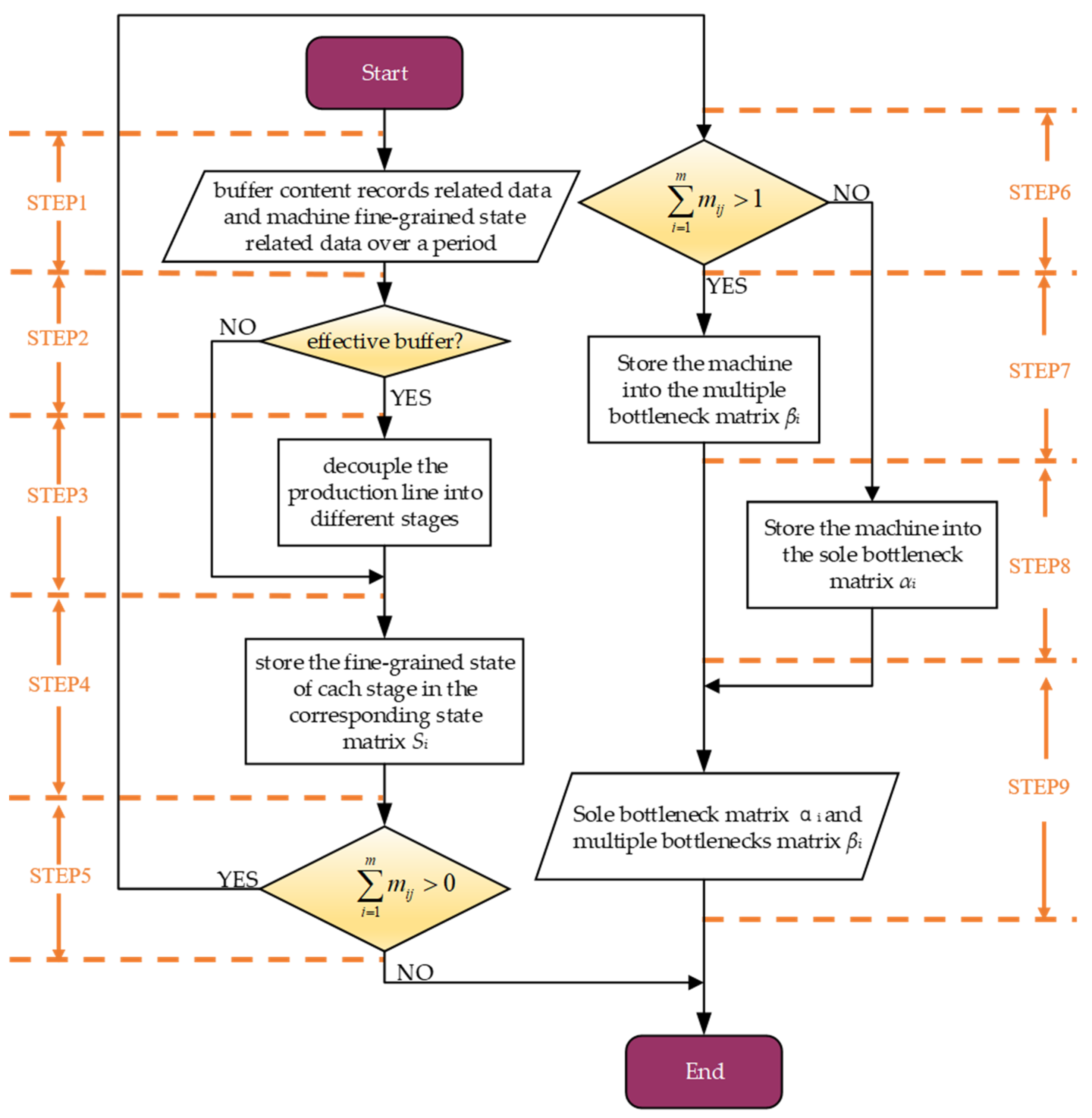
To present how the DBI-BS method is applied to detect bottlenecks, the workflow is illustrated as the following steps, as shown in Figure 1.
- (1)
- Acquire the current buffer content records-related data and machine fine-grained state-related data of period T. Here, t denotes the current time point. Go to decouple prediction line process and turn to step 2.
- (2)
- Judge whether the buffer in the system is effective or ineffective in this period. If the buffer is effective, turn to step 3, otherwise, turn to step 4. The method to find effective buffers is discussed in Section 3.1.
- (3)
- Decouple the production line into n + 1 stages according to the effective buffers in the system, then turn to step 4. The n is the number of effective buffers in the system. The method of decoupling the complex production line is discussed in Section 3.1.
- (4)
- Depending on the result of decoupling, the machines contained in the different stages are stored in the set Mi of machines for the i-th stage, and the fine-grained machine states are stored in the set Si of machine state for the i-th stage. Go to the bottleneck detection process, then turn to step 5.
- (5)
- Judge whether any machine in the system is in a valid state at time t. If there are machines in the system in a valid state, turn to step 6, otherwise, turn to the end.
- (6)
- Judge whether more than one machine in the system is in a valid state at time t. If more than one machine in the system is in a valid state, turn step 7, otherwise, turn to step 8.
- (7)
- Store the machines whose fine-grained states are valid at time t to the row corresponding to multiple bottleneck matrix βi, then turn to step 9.
- (8)
- Store the machine whose fine-grained state is valid at time t to the row corresponding to sole bottleneck matrix αi, then turn to step 9.
- (9)
- Output multiple bottleneck matrix βi and sole bottleneck matrix αi.
3.1. Complex Manufacturing System and Its Decoupling
3.1.1. Time Series Flow Modelling of CMS
CMS is an organizational system that is constructed to achieve a predetermined manufacturing purpose. It is an organic whole with specific functions composed of manufacturing processes, hardware, software, and related personnel. The CMS can be described as the workshop arranging to process j parts with a total of Nj. The complex system must complete the processing of the workpiece within the delivery period. For the convenience of discussion, the description of the symbols involved in the model are shown in Table 2.
The manufacturing process needs to meet the following constraints:
(1) Each process needs to be processed in order, according to the requirements of the process route of the workpiece;
(2) A workpiece can only be processed on one machine at the same time;
where xijk is one when the process Oij selects the machine Mk and xijk is zero when the process Oij does not select the machine Mk.
(3) One machine can only process one workpiece at the same time;
where sj(i+1) represents the processing completion time of the i procedure of the j-th workpiece, and it is also the processing start time of the i + 1-th procedure of the j-th workpiece; L presents a sufficiently large positive number.
In addition, there is a buffer with a specific capacity in front of each piece of equipment, and the equipment is unreliable. The processing time of the equipment to the workpiece is variable.
Assume the total time in an effective state of machine i can be expressed as:
Assume the set of bottleneck machines can be denoted as:
Abstractly represent the production activities involved in the manufacturing process as a manufacturing process time series flow model (MP-DataModel). MP-DataModel consists of multiple object data models (Ob-DataModel), and its description method is as follows:
where object represents the manufacturing process object and DSet represents the collected data generated by the object during the manufacturing process. DSet is time-series data, and its description method is:
3.1.2. Decoupling the CMS
Setting up buffers on the production line can improve system stability and output [40]. However, the decoupling effect of the buffer, taking the production line with the buffer as a whole to analyze the bottleneck, tends to cause confusion and misjudgment of the bottlenecks.
It should be noted that only effective buffers have the decoupling effect on the production system, so we must first find all effective buffer locations in the system. We define the effective buffer as the buffer that continues to act on the production system within the project time window [17]. Because when the buffer content reaches the limit value, the buffer loses its elasticity and cannot reduce the impact of the disturbance on the system. We define the buffers that arrive at the limit value within the project time window as invalid buffers. This article only considers the limited buffer, which shows that the buffer’s capacity is not unlimited.
Definition 1.
Effective buffer is a buffer that will never be full or empty within the project time window.
Assume the set of each buffer content records in different times for the manufacturing system can be denoted as:
Assume the matrix of buffers’ content records for the manufacturing system can be denoted as:
where m represents the number of time instances, n represents the number of buffers, and V represents the buffer matrix (10) of size m × n;
Definition 2.
Buffer j is the effective buffer in a system with n machines and m buffers during a period if:
Only the finite buffer is considered in this paper, which means the buffer capacity cannot be infinite. The effective buffering determination algorithm is proposed to find out the effective buffers of the system, as shown in Figure 2 and Figure 3. Then, the bottleneck state of each part should be identified by analyzing the fine-grained machine state of each part after decoupling. The overall bottleneck state of the production system should be obtained without confusion.
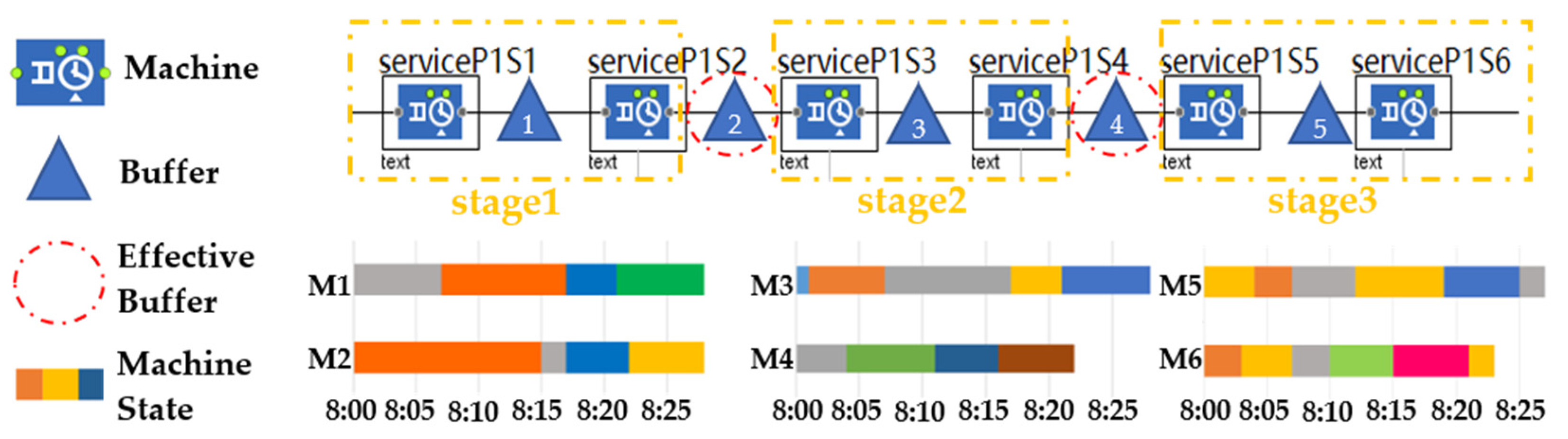
To explain the effective buffer, we present an example of a six-machine-five-buffer (6M5B) tandem line during one shift (shown in Figure 4). The buffer content information over the time interval is shown in Figure 5.
According to the buffer content information combined with the definition of an effective buffer, it can be known that B2 and B4, which never reached their limit, are the effective buffers of the system. The system is decoupled into three stages as shown in Figure 4: M1 and M2; M3 and M4; and M5 and M6, and each stage has its bottleneck state.
Assume the set of effective buffers for the manufacturing system can be denoted as:
In addition, assume the set of machines for the i-th stage can be denoted as:
3.2. Fine-Grained States of Manufacturing Resources
The current definition of manufacturing resources is not refined enough to meet the needs of dynamic bottleneck identification. This article summarizes nine fine-grained states that can be summarized into effective and ineffective states (shown in Figure 6) of manufacturing resources in manufacturing processing through the observation and analysis of the manufacturing process and inquiries to experienced operators. The effective state is when the machine aims to improve the system throughput, including the maintenance and service states. For example, a specific machine’s ongoing tasks may cause subsequent idle machines to wait, or the machine being repaired may block the previous machine.
The effect of the equipment status can be judged by whether the equipment status produces value. Table 3 explains the definition in detail and gives a classification of each state. All machines are in one of the nine given states at a given time.
Assume the set of effective states can be denoted as:
Assume the set of ineffective states can be denoted as:
Regarding several effective states that are adjacent in time as the effective continuous state, as shown in Figure 6, the duration of the total effective state is the sum of the duration of the individual effective states.
3.3. Dynamic Bottleneck Identification Method
The dynamic bottleneck identification method includes two parts: subsystem bottleneck identification and system-wide bottleneck identification. First, by analyzing the fine-grained state of the machines at each stage in the decoupled system, the bottleneck state of each subsystem is obtained. Then, the bottleneck of each subsystem is compared through the bottleneck quantification method to obtain the overall bottleneck of the production system.
3.3.1. Subsystem Bottleneck Identification
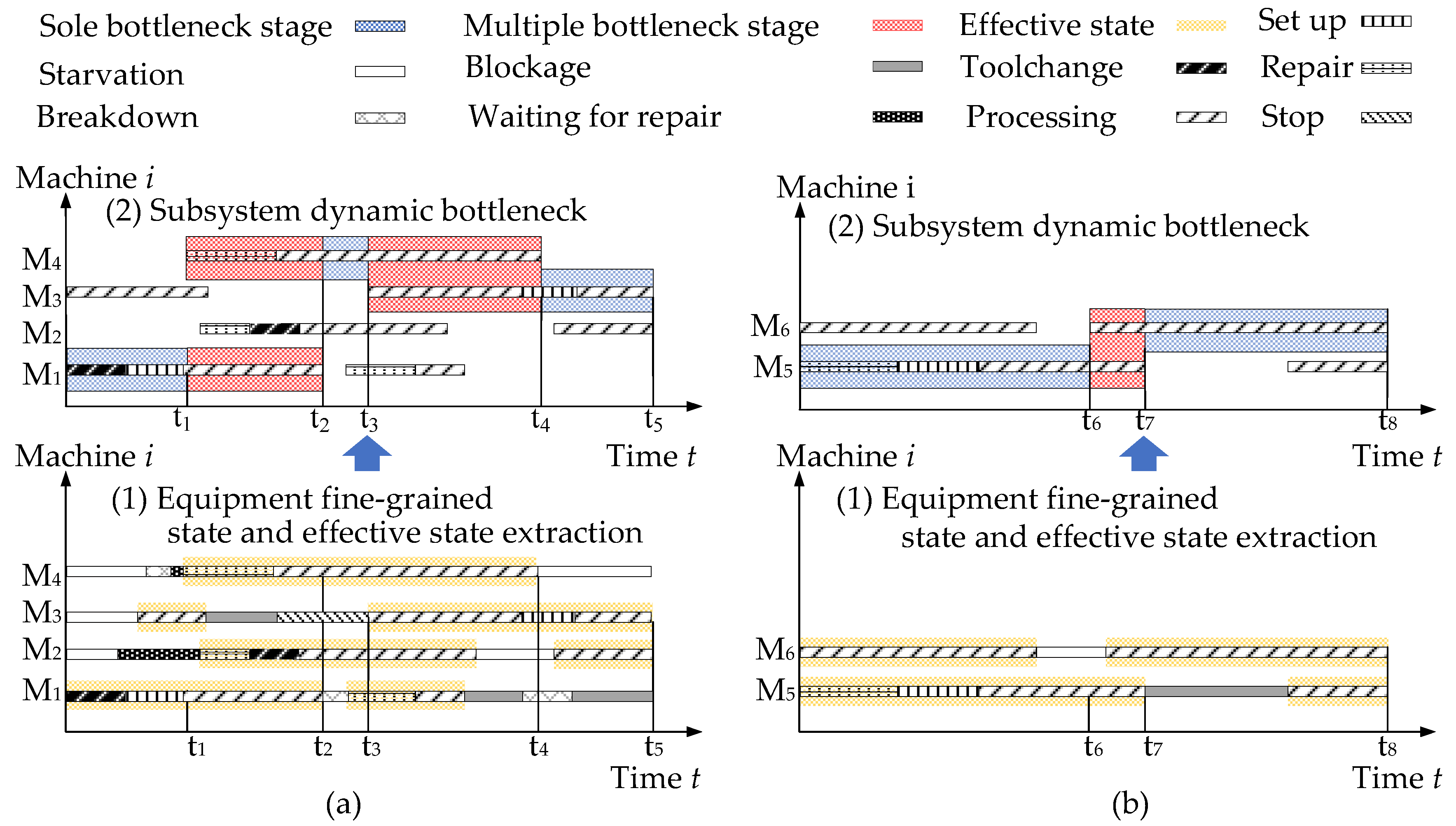
The bottleneck status of the system can be obtained by analyzing the fine-grained status of different machines over a period of time. A dynamic bottleneck detection algorithm is proposed to identify the bottleneck, as shown in Figure 7 and Figure 8.
Figure 9 shows an example of the bottleneck status of a subsystem over a period of time. During t1–t3, machine 4 is the bottleneck of the system; during t3–t5, machine 1 is the bottleneck of the system; and during t5–t7, machine 4 is the bottleneck of the system again.
3.3.2. System-Wide Bottleneck Identification
The bottleneck detection algorithm can identify the bottleneck of the subsystem in the CMS, but it cannot obtain the overall bottleneck status of the system. The system-wide bottleneck is critical to production management, so a multi-index real-time bottleneck degree calculation method (CFBI) is proposed to calculate the system bottleneck, as shown in formula (16). This method not only considers the independent characteristics of the machine (workload and capacity) but also considers the interaction between the machines (congestion and starvation caused by upstream and downstream machines) and improves it based on Lai et al. [7].
where gij represents the shifting bottleneck degree of station i in stage j, f1(t) represents the effective working time function, f2(t) represents the machine state function, and ω1 represents the system influence weight coefficient.
where ai represents the duration of the effective state in station i and amin represents the minimum value of the duration of the effective state of all machines in a particular stage.
where lij represents the preparing time of the task(part) j on station i, Pij represents the processing time of the task(part) j on station i, Ri represents the downtime of station i, and Mi represents the time to replace the required tooling for station i.
Assume the set of effective working times for all machines can be denoted as:
where Bi represents the blockage time of station i, Bi−1 represents the blockage time of the adjacent upstream station, Si represents the starvation time of station i, Si+1 represents the starvation time of the adjacent downstream station i + 1, and Zi represents the length of the current time window.
Assume the set of shifting bottleneck degrees for the ith machine can be denoted as:
The DBI-BS method is validated in a complex system composed of a simulated discrete manufacturing shop. The workshop is equipped with a cyber-physical system (CPS) that can collect real-time production data and uses the simulation software AnyLogic to build a one-to-one simulation model according to the structure of the physical workshop.
4. Results
This part includes four summaries: the simulation environment, CMS cases of a job shop, experimental study, and discussion. Using AnyLogic to build a simulation experiment environment for CMS is introduced in Section 4.1. This section explains how to generate shop floor agents and the logical relationship and illustrates the connection between the simulation model and the shop floor entities. Section 4.2 introduces a case of the CMS consisting of discrete manufacturing workshops equipped with a CPS that can collect real-time data of the production process. Section 4.3 is the results of the simulation experiments. These simulation experiments proved that the DBI-BS method could accurately identify the bottleneck in the CMS and the bottleneck movement phenomenon occurred. Section 4.4 discusses in detail the contribution of the proposed method to bottleneck identification methods and industrial practice.
4.1. Simulated Environment
AnyLogic enables users to provide the specific internals, process time, attributes, and resources required to complete each activity mentioned. A simulation model was constructed based on the structure of the physical workshop (deployed for three years with the same layout, the same number of workstations, and the same buffer area) to verify the performance of the DBI-BS method. As shown in Figure 10, the job shop case consists of six workstations, which can be simplified into a six-machine-five-buffer model (6M5B). The layout of the workshop and the simulation 3D model is shown in Figure 10. The detailed information of the workshop is detailed in Section 4.2.
The data required for model operation are obtained by analyzing the historical data of the actual workshop. In addition, some mathematical distributions commonly used in discrete simulation models are considered. MTTF\MTBF and machine breakdown obey the exponential distribution, and the processing time obeys the lognormal distribution. Queue simulates the queue (cache) where the entity is waiting for the next object to enter the storage area. The machine represents the manufacturing resource, and its fine-grained state can be expressed by related functions, such as the use of “maintenance ()” to define its maintenance status. The sink, usually at the end of the flow graph, is used to discard entities, representing the end of the processing process. The input of parts is in minutes. The analogue clock starts to work when the parts enter the system, and the input items are not restricted. The detailed expression of each agent is shown in Table 4.
The logical relationship between the agents is shown in Figure 11. Among them, the part agent and the machine agent are related through production tasks, and the parts and work-in-progress are related through the availability of parts. The parts processing on the machine and the parts to be processed in front of the machine reflect the WIP on the production line. In addition, the seven fine-grained states of manufacturing resources (fine-grained states 1–7) are related to the resource pool, and the remaining two fine-grained states (fine-grained state 8 and fine-grained state 9) are associated with the service queue.
4.2. CMS Case of Job Shop
The discrete manufacturing workshop, in this case, can process 13 kinds of parts. A real-time data collection scheme based on CPS is designed to realize a real-time collection of manufacturing process data. The acquisition equipment and its main parameters are shown in Table 5. The operating parameters of the CNC, spindle load, and other data are transmitted to the intelligent terminal through the ethernet port, the sensor is connected to the serial server through the RS485 cable in series, and the RFID reader is connected to the serial server through serial communication.
This experiment includes five processing parts: the brake disc, output shaft, traction wheel, coupling, and brake arm. The involved processing equipment includes the drilling and milling center (TC-R2B), precision machine tool (BNC427C), CNC lathe (L200E-M), facing turning center (LT2000EX), machining center (LJ-650), etc. The exact processing time of the workpiece is shown in Table 6.
4.3. Experimental Study
The test computer’s CPU frequency is 1.90GHz and 2.11 GHz, memory is 16GB, and the running environment is the Windows 10 operating system. By running the simulation system, the production process data of the CMS are obtained. This article selects a time window with a period of 300 min to analyze the bottleneck of the complex system after one week of simulation warm-up. Table 7 shows the buffer content data. It can be seen from the table that only buffer 4 is not full or empty during the simulation operation. According to the definition of an effective buffer, buffer 4 is effective, decoupling the system into two parts. The first part of the system comprises equipment 1, equipment 2, equipment 3, and equipment 4, and the second part is composed of equipment 5 and 6. Therefore, we first analyze the fine-grained status of the two subsystems and then analyze the overall bottleneck situation of the system through CFBI.
After processing the simulation data, the dynamic bottleneck state of the CMS is obtained, as shown in the Figure 12. Take Subsystem 1 as an example to explain the dynamic bottleneck phenomenon in the production process. First, the fine-grained state of the equipment is analyzed and the effective state is extracted. The yellow area in Figure 12a(1) is the effective fine-grained state of the extracted machine. Then, the overall bottleneck status of the subsystem according to the effective status is obtained, as shown in Figure 12a(2), where the blue area is a single bottleneck stage, and the red zone is a multi-bottleneck stage. Different bottleneck stages divide the time window into several segments. For each segment, the CFBI is used to calculate the comprehensive bottleneck of the equipment. The calculation results are shown in Table 8. The bold parts in the table are the system bottlenecks in the corresponding period. The calculation results of the bottleneck degree are consistent with the results of the dynamic bottleneck identification method shown in Figure 12, proving that the proposed method is effective. In the same period, the comprehensive bottleneck degree of different machines is different, which indicates that different machines have different degrees of restriction on the system. Therefore, system resources should be allocated according to the bottleneck to maximize system benefits. In addition, it can be seen that the bottleneck machines are different in different periods, which indicates that the bottleneck has moved.
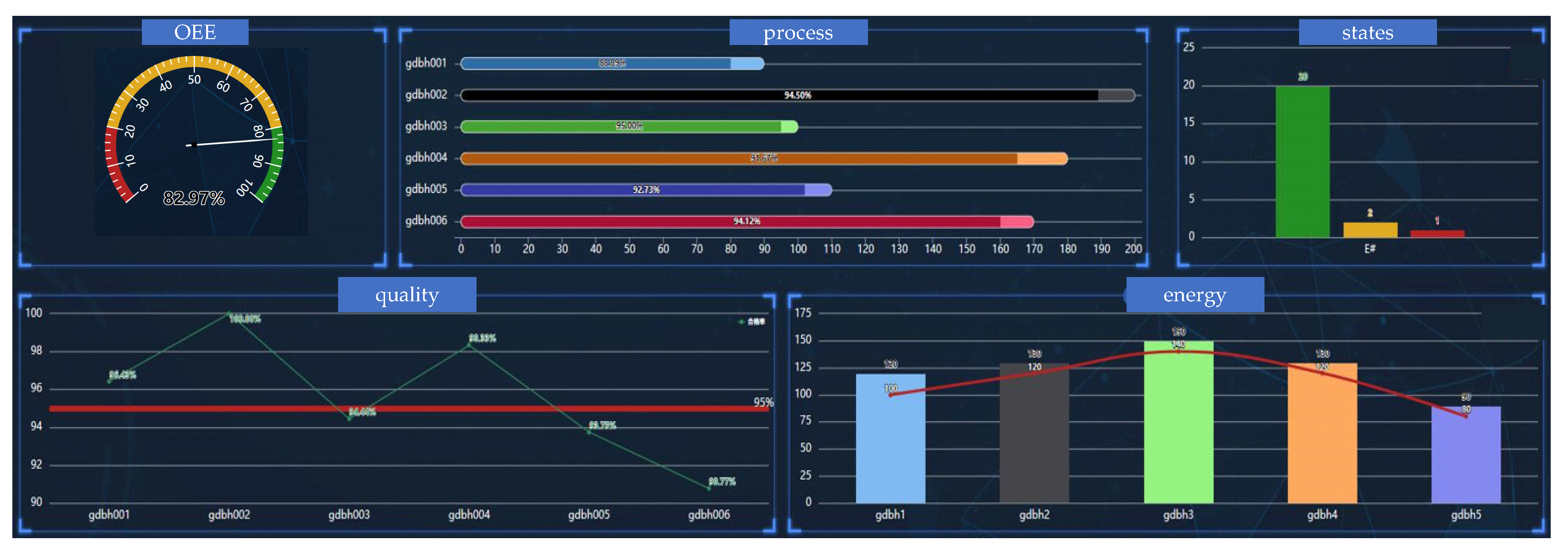
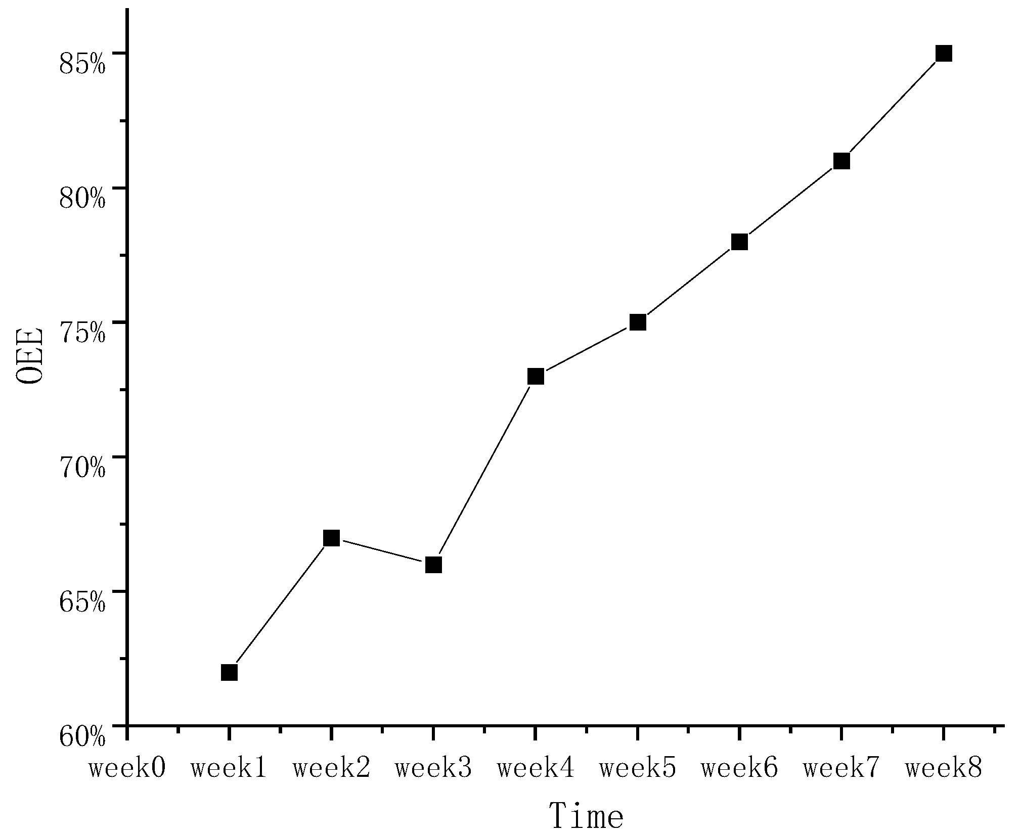
The ultimate goal of identifying bottlenecks is to improve the production capacity of complex manufacturing systems, and OEE is an effective indicator to evaluate the system’s production capacity. The elevator parts manufacturing enterprise guides the optimization of the production process according to the results of the dynamic bottleneck identification, such as improving the capacity of the bottleneck machine by optimizing the buffer configuration, enhancing the priority of maintenance, and dynamically allocating manufacturing resources, and the OEE of the system has been steadily improved. The target level has been reached, about 85% per day. Figure 13 shows the OEE screen of the workshop, and Figure 14 shows the weekly average daily OEE of the production line in the past two months.
4.4. Discussion
This paper proposes a dynamic bottleneck identification framework that is driven by simulation data, including effective buffer identification, global and subsystem bottleneck identification, and comprehensive bottleneck degree calculation. The method can dynamically identify bottlenecks in complex manufacturing systems and improve system output to target levels.
Most identification methods consider bottlenecks independently, and there are few studies on identification from a system perspective. Considering the strong coupling between the elements in CMS, this paper proposes a method of decoupling CMS through effective buffering and studies the identification method of effective buffering. The active state duration is used to define the bottleneck for the problem of inaccurate state division, nine fine-grained states that can be classified into two categories are given in combination with the actual production situation, and detailed definitions are given. In addition, a time series flow model of the manufacturing states is established to process state data for dynamic bottleneck identification, and a comprehensive bottleneck degree model is proposed to quantify different bottlenecks of system resources.
Compared with the existing simulation-based identification methods, a real-time data acquisition scheme based on CPS is designed to realize the real-time acquisition of manufacturing process data and use them as the data source of the simulation model. By studying the one-to-one mapping relationship between workshop entities and simulation agents, a CMS simulation model closer to the actual production situation is established. Time-varying production data collected through the manufacturing IoT can help in understanding the dynamic operations of the shop floor without relying on ideal mathematical distributions.
The dynamic bottleneck identification method proposed in this paper has the following advantages. First, the process can be completed automatically, with high analysis efficiency and objective results; second, by dividing the CMS into different stages and further subdividing the equipment status to reduce the coupling of the system reduces the probability of misjudging bottlenecks. In addition, the sole-bottleneck and multi-bottleneck stages of the system can be seen through the duration of the fine-grained state of the machine, and the process of bottleneck movement can be presented. Finally, accurate production data and simulation models can cost-effectively guide the actual production process. Managers can identify the bottlenecks limiting system output based on historical production data. The idea of a hybrid drive can provide a valuable reference for digital twin technology in Industry 4.0.
5. Conclusions
This paper introduces a dynamic bottleneck identification method based on the fine-grained state of manufacturing resources. It combines the decoupling method of complex systems to improve the accuracy of bottleneck identification. In addition, because the bottleneck between the subsystems cannot be compared, a comprehensive mobile bottleneck degree CFBI method is proposed to calculate the bottleneck degree of the bottleneck equipment of the subsystem and then obtain the overall bottleneck situation the system. The main contributions of this article include:
- (1)
- The decoupling effect of the buffer on the production line is clarified, and a method to use an effective buffer to decouple the CMS is proposed.
- (2)
- Based on the active time method, the state of manufacturing resources is further divided into a fine-grained granularity. A dynamic bottleneck identification method is proposed based on the fine-grained state of equipment.
- (3)
- Aiming at the problem that the bottlenecks between different subsystems cannot be directly compared, comprehensively considering the operating status of the system and the mutual influence between each device, a comprehensive bottleneck degree index is constructed to evaluate the overall bottleneck status of the system.
The DBI-BS method establishes the connection between the real-time data of the manufacturing process and the system bottleneck. Future research work will be carried out in predicting the bottleneck by the machine learning method and to further explore the impact of system bottlenecks on the total output of the production system.
Author Contributions
Conceptualization, X.S.; Data curation, X.S.; Formal analysis, X.S.; Funding acquisition, W.J.; Investigation, C.C.; Methodology, X.S.; Resources, W.J.; Validation, J.Y.; Writing—original draft, X.S.; Writing—review and editing, J.L. All authors have read and agreed to the published version of the manuscript.
Funding
This research was funded by the Major Scientific and Technological Innovation Project of Shandong Province, grant number 2019JZZY020111.
Institutional Review Board Statement
Not applicable.
Informed Consent Statement
Not applicable.
Conflicts of Interest
The authors declare no conflict of interest.
References
- Zhang, C.; Jiang, P. RFID-driven energy-efficient control approach of CNC machine tools using deep belief networks. IEEE Trans. Autom. Sci. Eng. 2019, 17, 129–141. [Google Scholar] [CrossRef]
- Zhou, G.; Zhang, C.; Li, Z.; Ding, K.; Wang, C. Knowledge-driven digital twin manufacturing cell towards intelligent manufacturing. Int. J. Prod. Res. 2020, 58, 1034–1051. [Google Scholar] [CrossRef]
- Zhang, C.; Ji, W. Big data analysis approach for real-time carbon efficiency evaluation of discrete manufacturing workshops. IEEE Access 2019, 7, 107730–107743. [Google Scholar] [CrossRef]
- Wang, J.; Li, Y.; Zhao, R.; Gao, R.X. Physics guided neural network for machining tool wear prediction. J. Manuf. Syst. 2020, 57, 298–310. [Google Scholar] [CrossRef]
- Zhang, C.; Wang, Z.; Ding, K.; Chan, F.T.; Ji, W. An energy-aware cyber physical system for energy Big data analysis and recessive production anomalies detection in discrete manufacturing workshops. Int. J. Prod. Res. 2020, 58, 7059–7077. [Google Scholar] [CrossRef]
- Kuo, T.; Hsu, N.; Li, T.Y.; Chao, C. Industry 4.0 enabling manufacturing competitiveness: Delivery performance improvement based on theory of constraints. J. Manuf. Syst. 2021, 60, 152–161. [Google Scholar] [CrossRef]
- Lai, X.; Shui, H.; Ding, D.; Ni, J. Data-driven dynamic bottleneck detection in complex manufacturing systems. J. Manuf. Syst. 2021, 60, 662–675. [Google Scholar] [CrossRef]
- Khalid, M.N.A.; Yusof, U.K. Incorporating shifting bottleneck identification in assembly line balancing problem using an artificial immune system approach. Flex. Serv. Manuf. J. 2020, 33, 717–749. [Google Scholar] [CrossRef]
- Ikeziri, L.M.; Souza, F.B.D.; Gupta, M.C.; de Camargo Fiorini, P. Theory of constraints: Review and bibliometric analysis. Int. J. Prod. Res. 2019, 57, 5068–5102. [Google Scholar] [CrossRef] [Green Version]
- Bernedixen, J. Automated Bottleneck Analysis of Production Systems: Increasing the Applicability of Simulation-Based Multi-Objective Optimization for Bottleneck Analysis within Industry. Ph.D. Thesis, University of Skövde, Högskolevägen, Sweden, 2018. [Google Scholar]
- Wang, J.; Chen, J.; Zhang, Y.; Huang, G.Q. Schedule-based execution bottleneck identification in a job shop. Comput. Ind. Eng. 2016, 98, 308–322. [Google Scholar] [CrossRef]
- Braune, R.; Zäpfel, G. Shifting bottleneck scheduling for total weighted tardiness minimization—A computational evaluation of subproblem and re-optimization heuristics. Comput. Oper. Res. 2016, 66, 130–140. [Google Scholar] [CrossRef]
- Huang, B.; Wang, W.; Ren, S.; Zhong, R.Y.; Jiang, J. A proactive task dispatching method based on future bottleneck prediction for the smart factory. Int. J. Comput. Integr. Manuf. 2019, 32, 278–293. [Google Scholar] [CrossRef]
- Subramaniyan, M.; Skoogh, A.; Muhammad, A.S.; Bokrantz, J.; Bekar, E.T. A prognostic algorithm to prescribe improvement measures on throughput bottlenecks. J. Manuf. Syst. 2019, 53, 271–281. [Google Scholar] [CrossRef]
- Fang, W.; Guo, Y.; Liao, W.; Huang, S.; Yang, N.; Liu, J. A Parallel Gated Recurrent Units (P-GRUs) network for the shifting lateness bottleneck prediction in make-to-order production system. Comput. Ind. Eng. 2020, 140, 106246. [Google Scholar] [CrossRef]
- Subramaniyan, M.; Skoogh, A.; Gopalakrishnan, M.; Hanna, A. Real-time data-driven average active period method for bottleneck detection. Int. J. Des. Nat. Ecodynamics 2016, 11, 428–437. [Google Scholar] [CrossRef] [Green Version]
- Li, L.; Chang, Q.; Ni, J. Data driven bottleneck detection of manufacturing systems. Int. J. Prod. Res. 2009, 47, 5019–5036. [Google Scholar] [CrossRef]
- Gu, X.; Jin, X.; Guo, W.; Ni, J. Estimation of active maintenance opportunity windows in Bernoulli production lines. J. Manuf. Syst. 2017, 45, 109–120. [Google Scholar] [CrossRef]
- Li, J.; Meerkov, S.M. Bottlenecks with respect to due-time performance in pull serial production lines, Proceedings 2000 ICRA. Millennium Conference. IEEE Int. Conf. Robot. Autom. 2000, 3, 2635–2640. [Google Scholar]
- Li, L. Bottleneck detection of complex manufacturing systems using a data-driven method. Int. J. Prod. Res. 2009, 47, 6929–6940. [Google Scholar] [CrossRef]
- Dong, Y.; Ma, J.; Wang, S.; Liu, T.; Chen, X.; Huang, H. An Accurate Small Signal Dynamic Model for LCC-HVDC. IEEE Trans. Appl. Supercon. 2021, 31, 1–6. [Google Scholar] [CrossRef]
- Qiu, Y.; Sawhney, R.; Zhang, C.; Chen, S.; Zhang, T.; Lisar, V.G.; Jiang, K.; Ji, W. Data mining–based disturbances prediction for job shop scheduling. Adv. Mech. Eng. 2019, 11, 753307422. [Google Scholar] [CrossRef]
- Sun, K.; Qiu, W.; Yao, W.; You, S.; Yin, H.; Liu, Y. Frequency injection based hvdc attack-defense control via squeeze-excitation double cnn. IEEE Trans. Power Syst. 2021, 36, 5305–5316. [Google Scholar] [CrossRef]
- Subramaniyan, M.; Skoogh, A.; Gopalakrishnan, M.; Salomonsson, H.; Hanna, A.; Lämkull, D. An algorithm for data-driven shifting bottleneck detection. Cogent Eng. 2016, 3, 1239516. [Google Scholar] [CrossRef]
- Chen, J.; Wang, J.; Du, X. Shifting bottleneck-driven TOCh for solving product mix problems. Int. J. Prod. Res. 2020, 59, 5558–5577. [Google Scholar] [CrossRef]
- Chang, Q.; Biller, S.; Xiao, G. Transient analysis of downtimes and bottleneck dynamics in serial manufacturing systems. J. Manuf. Sci. Eng. 2010, 132, 051015. [Google Scholar] [CrossRef]
- Gu, X.; Jin, X.; Ni, J. Prediction of passive maintenance opportunity windows on bottleneck machines in complex manufacturing systems. J. Manuf. Sci. Eng. 2015, 137, 031017. [Google Scholar] [CrossRef]
- Wedel, M.; Noessler, P.; Metternich, J. Development of bottleneck detection methods allowing for an effective fault repair prioritization in machining lines of the automobile industry. Prod. Eng. 2016, 10, 329–336. [Google Scholar] [CrossRef]
- Sun, K.; Li, K.; Zhang, Z.; Liang, Y.; Liu, Z.; Lee, W. An integration planning for renewable energies, hydrogen plant and logistics center in the suburban power grid. IEEE Trans. Ind. Appl. 2021, 58, 2771–2779. [Google Scholar] [CrossRef]
- Li, L.; Chang, Q.; Xiao, G.; Ambani, S. Throughput bottleneck prediction of manufacturing systems using time series analysis. J. Manuf. Sci. Eng. 2011, 133, 021015. [Google Scholar] [CrossRef]
- Alden, J.M.; Burns, L.D.; Costy, T.; Hutton, R.D.; Jackson, C.A.; Kim, D.S.; Kohls, K.A.; Owen, J.H.; Turnquist, M.A.; Veen, D.J.V. General Motors increases its production throughput. Interfaces 2006, 36, 6–25. [Google Scholar] [CrossRef]
- Roser, C.; Nakano, M.; Tanaka, M. Shifting bottleneck detection. In Proceedings of the Winter Simulation Conference, San Diego, CA, USA, 8–11 December 2002; Volume 2, pp. 1079–1086. [Google Scholar]
- Law, A.M.; Kelton, W.D.; Kelton, W.D. Simulation Modeling and Analysis; McGraw-Hill: New York, NY, USA, 2000. [Google Scholar]
- Chang, Q.; Ni, J.; Bandyopadhyay, P.; Biller, S.; Xiao, G. Supervisory factory control based on real-time production feedback. J. Manuf. Sci. Eng. 2007, 129, 653–660. [Google Scholar] [CrossRef]
- Nahmias, S.; Cheng, Y. Production and Operations Analysis; McGraw-hill: New York, NY, USA, 2001. [Google Scholar]
- Liu, M.; Tang, J.; Ge, M.; Jiang, Z.; Hu, J.; Ling, L. Dynamic prediction method of production logistics bottleneck based on bottleneck index. Chin. J. Mech. Eng. Engl. Ed. 2009, 22, 710–716. [Google Scholar] [CrossRef]
- Roser, C.; Lorentzen, K.; Deuse, J. Reliable shop floor bottleneck detection for flow lines through process and inventory observations. Procedia CIRP 2014, 19, 63–68. [Google Scholar] [CrossRef] [Green Version]
- Roser, C.; Nakano, M.; Tanaka, M. Monitoring bottlenecks in dynamic discrete event systems. In Proceedings of the European Simulation Multiconference, Magdeburg, Germany, 25–27 October 2004. [Google Scholar]
- Subramaniyan, M.; Skoogh, A.; Muhammad, A.S.; Bokrantz, J.; Johansson, B.; Roser, C. A generic hierarchical clustering approach for detecting bottlenecks in manufacturing. J. Manuf. Syst. 2020, 55, 143–158. [Google Scholar] [CrossRef]
- Tsadiras, A.K.; Papadopoulos, C.T.; O Kelly, M.E. An artificial neural network based decision support system for solving the buffer allocation problem in reliable production lines. Comput. Ind. Eng. 2013, 66, 1150–1162. [Google Scholar] [CrossRef]
Figure 1.
DBI-BS method flowchart.

Figure 2.
The effective buffering determination algorithm.

Figure 3.
The effective buffering determination flowchart.

Figure 4.
The six-machine-five-buffer (6M5B) tandem line.

Figure 5.
The buffer content information.

Figure 6.
Effective states and ineffective states of the machine.

Figure 7.
The dynamic bottleneck recognition algorithm.

Figure 8.
The dynamic bottleneck recognition flowchart.

Figure 9.
Example of subsystem bottleneck status.

Figure 10.
The layout of the discrete smart shop floor and simulation model.

Figure 11.
The logical relationship between agents.

Figure 12.
Complex system dynamic bottleneck identification. (a) Subsystem 1 dynamic bottleneck identification; (b) Subsystem 2 dynamic bottleneck identification.
Figure 12.
Complex system dynamic bottleneck identification. (a) Subsystem 1 dynamic bottleneck identification; (b) Subsystem 2 dynamic bottleneck identification.

Figure 13.
The OEE screen of the workshop.

Figure 14.
The weekly average daily OEE.

Table 2.
Summary of bottleneck identification.
| Symbol | Description |
|---|---|
| j, i, k | sequence numbers of workpiece, process, and machine |
| Nj, Ni, m | number of workpieces, processes, and machines |
| Sij, Cij | the start and completion time of the i-th process of the j-th workpiece |
| tqs, tqe | the processing start time and end time of the active state |
| Pijh | the processing time of the i-th process of the j-th workpiece on the machine h |
| Sul | the processing start time of the l-th process of the u-th workpiece; |
| xijk | the decision variable for the machine selection of the process |
| yijhkl | the decision variable is selected for the procedure |
| gij | the shifting bottleneck degree of station i in time window j |
| v(anm) | the value of the m-th attribute under scene c at time n |
| ctn | the scene at time n |
Table 3.
Fine-grained states of manufacturing resources.
| State | Definition | Categories | |
|---|---|---|---|
| 1 | Producing | The machine is processing products. | Effective machine states |
| 2 | Set up | Preparing a machine for its next run after it has completed producing the last part of the previous run | |
| 3 | Tool change | Replacing the required tooling for the equipment | |
| 4 | Repair | basic maintenance tasks, such as checking, testing, lubricating, and replacing worn or damaged parts on a planned and ongoing basis. | |
| 5 | Breakdown | The period during which equipment or machine is not functional or cannot work | Ineffective machine states |
| 6 | Waiting for Repair | Waiting time between machine breakdown and maintenance | |
| 7 | Stop | Waiting beyond starvation and blockages that cannot increase system output, such as employee absenteeism | |
| 8 | Blockage | The machine is idle because it cannot transport WIP downstream. | |
| 9 | Starvation | The machine is idle due to a lack of WIP from upstream. |
Table 4.
Created Module Parameters.
| Object Name | Entity Type | Agent Name | Attributes |
|---|---|---|---|
| Part | Source | sourcePart | Agent (); Advanced (); Actions () |
| Process | Service | ServiceP1 | Resource sets (); Delay time (); Advanced (); Actions (); Maximum queue capacity (); |
| End of process | Sink | sinkPart | Action (); Advanced () |
| Machine | Resource Pool | rpStation | Shifts (); Breaks (); Failures (); Maintenance (); Advanced (); Actions () |
| Event | Timeout | eventUtiPerHr | Actions () |
| WIP | Parameter | pWIPPart | Value editor (); Advanced () |
| Production Plan | Schedule | schedulepart | Data (); Action (); Exceptions (); Preview (); Advanced () |
Table 5.
Data collection equipment and main parameters.
| Machine | Collection Object | Technical Parameter |
|---|---|---|
| Sensor (PCB356A03) | Vibration signal | The sampling upper limit frequency is 36 KHz. |
| Data acquisition card (NI9234) | Acoustic signal Vibration signal | The sampling upper limit frequency is 51.2 KHz. The dynamic range is 102 DB. |
| Machining Center | Processing parameters, Spindle load, etc. | XYZ axis maximum stroke, main motor power, spindle speed, positioning accuracy |
| High-frequency reader (ALR-F800) | RFID Label | IP64 level waterproof/dustproof |
| ALR-8696 antenna | RFID Label | Working range 865 HZ–960 HZ |
Table 6.
Parts processing information.
| Workpiece Category | Planned Processing Time (s) | |||||
|---|---|---|---|---|---|---|
| M1 | M2 | M3 | M4 | M5 | M6 | |
| Brake disc | 18 | - | 24 | - | 42 | - |
| Output shaft | - | 18 | - | 18 | - | 84 |
| Traction wheel | 48 | - | 24 | - | - | 98 |
| Coupling | - | 30 | 24 | - | 78 | - |
| Brake arm | 36 | - | 42 | - | - | - |
Table 7.
Buffer capacity change table.
| Time (min) | Buffer1 | Buffer2 | Buffer3 | Buffer4 | Buffer5 |
|---|---|---|---|---|---|
| 1 | 6 | 2 | 10 | 2 | 3 |
| 2 | 7 | 0 | 10 | 2 | 0 |
| 3 | 7 | 0 | 7 | 6 | 0 |
| 4 | 8 | 3 | 5 | 7 | 2 |
| 5 | 10 | 5 | 5 | 6 | 5 |
| 6 | 10 | 5 | 5 | 2 | 6 |
| 7 | 7 | 3 | 5 | 2 | 6 |
| ··· | ··· | ··· | ··· | ··· | ··· |
| 188 | 5 | 10 | 5 | 7 | 5 |
| 189 | 5 | 10 | 6 | 7 | 5 |
| 190 | 3 | 0 | 6 | 6 | 10 |
| 191 | 0 | 0 | 6 | 6 | 10 |
| ··· | ··· | ··· | ··· | ··· | ··· |
| 299 | 5 | 8 | 5 | 7 | 10 |
| 300 | 4 | 10 | 6 | 5 | 10 |
Table 8.
Data of subsystem bottleneck.
| Machine i | Li | Pi | Ri | Mi | Bi | Si | CFBI | |
|---|---|---|---|---|---|---|---|---|
| t0–t1 | M1 | 0 | 32 | 0 | 28 | 0 | 0 | 0.6033 |
| M2 | 0 | 0 | 0 | 0 | 0 | 26 | 0.0467 | |
| M3 | 60 | 0 | 0 | 0 | 0 | 30 | 0.3233 | |
| M4 | 0 | 0 | 0 | 0 | 0 | 32 | 0 | |
| t1–t2 | M1 | 73 | 0 | 0 | 0 | 0 | 0 | 1.6846 |
| M2 | 13 | 23 | 0 | 25 | 0 | 0 | 1.4077 | |
| M3 | 13 | 0 | 0 | 0 | 0 | 0 | 0.3000 | |
| M4 | 22 | 51 | 0 | 0 | 0 | 0 | 1.6846 | |
| t2–t3 | M1 | 0 | 0 | 12 | 0 | 0 | 0 | 0.3000 |
| M2 | 20 | 0 | 0 | 0 | 0 | 0 | 0.5000 | |
| M3 | 0 | 0 | 0 | 0 | 0 | 0 | 0 | |
| M4 | 22 | 0 | 0 | 0 | 0 | 0 | 0.5500 | |
| t3–t4 | M1 | 26 | 0 | 24 | 0 | 34 | 0 | 0.6295 |
| M2 | 40 | 0 | 0 | 0 | 0 | 32 | 0.3159 | |
| M3 | 78 | 10 | 0 | 0 | 0 | 0 | 0.6600 | |
| M4 | 88 | 0 | 0 | 0 | 0 | 0 | 0.6600 | |
| t4–t5 | M1 | 0 | 0 | 0 | 0 | 41 | 0 | 0.0982 |
| M2 | 52 | 0 | 0 | 0 | 0 | 8 | 0.7053 | |
| M3 | 39 | 19 | 0 | 0 | 0 | 0 | 1.0346 | |
| M4 | 0 | 0 | 0 | 0 | 0 | 57 | 0 | |
Publisher’s Note: MDPI stays neutral with regard to jurisdictional claims in published maps and institutional affiliations. |
© 2022 by the authors. Licensee MDPI, Basel, Switzerland. This article is an open access article distributed under the terms and conditions of the Creative Commons Attribution (CC BY) license (https://creativecommons.org/licenses/by/4.0/).
Share and Cite
MDPI and ACS Style
Su, X.; Lu, J.; Chen, C.; Yu, J.; Ji, W. Dynamic Bottleneck Identification of Manufacturing Resources in Complex Manufacturing System. Appl. Sci. 2022, 12, 4195. https://0-doi-org.brum.beds.ac.uk/10.3390/app12094195
AMA Style
Su X, Lu J, Chen C, Yu J, Ji W. Dynamic Bottleneck Identification of Manufacturing Resources in Complex Manufacturing System. Applied Sciences. 2022; 12(9):4195. https://0-doi-org.brum.beds.ac.uk/10.3390/app12094195
Chicago/Turabian StyleSu, Xuan, Jingyu Lu, Chen Chen, Junjie Yu, and Weixi Ji. 2022. "Dynamic Bottleneck Identification of Manufacturing Resources in Complex Manufacturing System" Applied Sciences 12, no. 9: 4195. https://0-doi-org.brum.beds.ac.uk/10.3390/app12094195
Note that from the first issue of 2016, this journal uses article numbers instead of page numbers. See further details here.