Article

A Comparative Energy and Economic Analysis of Different Solar Thermal Domestic Hot Water Systems for the Greek Climate Zones: A Multi-Objective Evaluation Approach

Department of Mechanical Engineering Educators, School of Pedagogical and Technological Education (ASPETE), Attika, 14121 Irakleio, Greece
*
Author to whom correspondence should be addressed.
Submission received: 14 April 2022 / Revised: 26 April 2022 / Accepted: 29 April 2022 / Published: 30 April 2022
(This article belongs to the Special Issue Advances in the Evaluation of Advanced Energy Conversion Systems)

Abstract

:
The exploitation of solar irradiation in the building sector is a promising way to achieve decarbonization and reduce the operating costs of the building. The potential of solar energy in Greece is high and therefore this idea can lead to excellent results. In this direction, the goal of the present analysis is the detailed investigation of different solar thermal systems for domestic hot water production in the different climate zones of Greece. Four typical cities are studied in order to examine the climate zones A, B, C, and D, while three different solar thermal collectors coupled to insulated storage tanks are studied for every city. The simple flat plate collector, the advanced flat plate collector, and the evacuated tube collector are the selected solar systems for the present work. The climate data and the characteristics of the solar thermal systems follow the Greek Chamber regulations known as “KENAK”. The analysis is conducted by following the well-known f-chart method and every design is optimized by using energy and financial criteria. The final design is determined by conducting a multi-objective evaluation methodology. It is notable to state that the collector slope and the collecting area are important parameters of this work, while the study case regards a building with 30 residents. According to the final results, the advanced flat plate collector is the best choice according to the multi-objective evaluation procedure.

1. Introduction

The sustainable development goals for the Agenda 2030 [1] aim to make the cities sustainable and to increase affordable and clean energy. In this direction, the exploitation of renewable sources like solar irradiation, wind potential, and biomass is a critical factor in achieving these goals [2]. Buildings are important energy consumers with 40% of the worldwide energy consumption to be done on them, while one-third of the global greenhouse gas emissions are produced for covering the Buildings’ needs [3]. Thus, the proper utilization of renewable energies in the building sector is an ideal idea in order to make future buildings environmentally friendlier and financially viable [4]. Especially, solar irradiation can be exploited in the building sector in various ways like solar thermal systems for domestic hot water (DHW) production, solar thermal units for space heating, and photovoltaics for electricity production [5].
Domestic hot water production consists of a critical energy need of the buildings which exists during all the year period [6] and thus the exploitation of solar energy for covering this demand can lead to great advantages regarding energy savings [7]. Solar coverage is a critical parameter that indicates the faction of the demand that is covered by the solar energy [8], while the other part is covered by an auxiliary source, usually electrical resistance, or fuel boiler. Usually, a typical family can cover the majority of the DHW needs with a collecting area of around 2–2.5 m2 and a tank of 150–200 L [9]. However, these are general rules and there is a need for more accurate design, especially in greater buildings and in central systems with many residents.
Regarding, the solar collector types, the use of a flat plate collector (FPC) is the most usual choice [10], while the selection of an evacuated tube collector (ETC is an alternative, especially in cold regions [11]. In the domain of storage tanks, sensible heat storage is the most usual choice [12], while there are ideas about using latent storage with phase change materials [13]. Moreover, it is useful to state that another idea is the incorporation of the tank inside the collector [14]; a compact design that has lower efficiency than conventional systems. Last but not least, solar thermal technologies can be combined with heat pumps for producing DHW [15].
Greece is a country with a high solar potential which is estimated at 1750 kWh/m2 [16] for a 45° tilted surface in Athens, while similar values are obtained for other locations. Moreover, Greece is a country where the utilization of solar thermal systems for building applications is a socially acceptable technology [17] with social and environmental benefits [18], so the further installation of solar thermal systems in Greece is something that is feasible. Moreover, Tsilingiridis and Martinopoulos [19] conducted a study based on a 30-year experience with solar thermal units and they found that there is an important reduction in CO2 emissions due to the solar irradiation exploitation in Greece. In another work, Koroneos and Nanaki [20] stated that the environmental impact during the construction of the solar thermal collectors is relatively low and so the life cycle assessment is positive. Furthermore, they concluded that the payback period has an acceptable value of close to 5 years. Another environmental work about the solar thermal systems in Greece by Martinopoulos et al. [21] shows that the initial materials and the construction techniques of these systems have a low impact on the overall system’s environmental performance. Thus, the energy analysis of the solar thermal systems is the critical factor that determines both their energy and their environmental characterization of them. In this direction, Balaras et al. [22] found that the solar thermal units for domestic hot water production can lead to important energy reduction for the Greek climate conditions. Antoniadis and Martinopoulos [23] conducted an optimization study with TRNSYS software about the use of FPC on a solar system for space heating and domestic hot water for the location of Thessaloniki (Zone C in Greece). They calculated the overall seasonal solar fraction to be around 39%. In another approach based on the ISO 9459-2, Bellos and Tzivanidis [24] studied a solar thermal system for DHW in Athens (Zone B in Greece) and they calculated the average annual thermal efficiency at 54%, the payback period at 5 years, while the internal rate of return close to 20%.
The previous summary of literature studies shows that there is a great interest in solar thermal systems for DHW in the Greek building sector. Various studies have been performed in order to determine the energy and the economic performance of these systems. However, there is not any study that investigates different solar thermal collector types for different locations in order to present the optimal designs in a systematic way for all the climate zones of Greece. In this direction, the present analysis covers this gap by conducting a systematic analysis by comparing different designs of three different solar thermal collectors for the four climate zones of Greece. Parametric analysis and optimization procedures are performed in order to conduct multilateral work based on energy and economic criteria. The final results of this study can be used for the suitable selection of the collector type, its slope, and its collecting area according to the examined location. So, the results of this work can act as guidelines for the future installations of solar thermal units in Greece in order to maximize the renewable share, maximize the energy savings and maximize the environmental benefits from solar energy exploitation.

2. Material and Methods

Section 2 includes the details of the examined configuration, the used mathematical background, and the followed methodology.

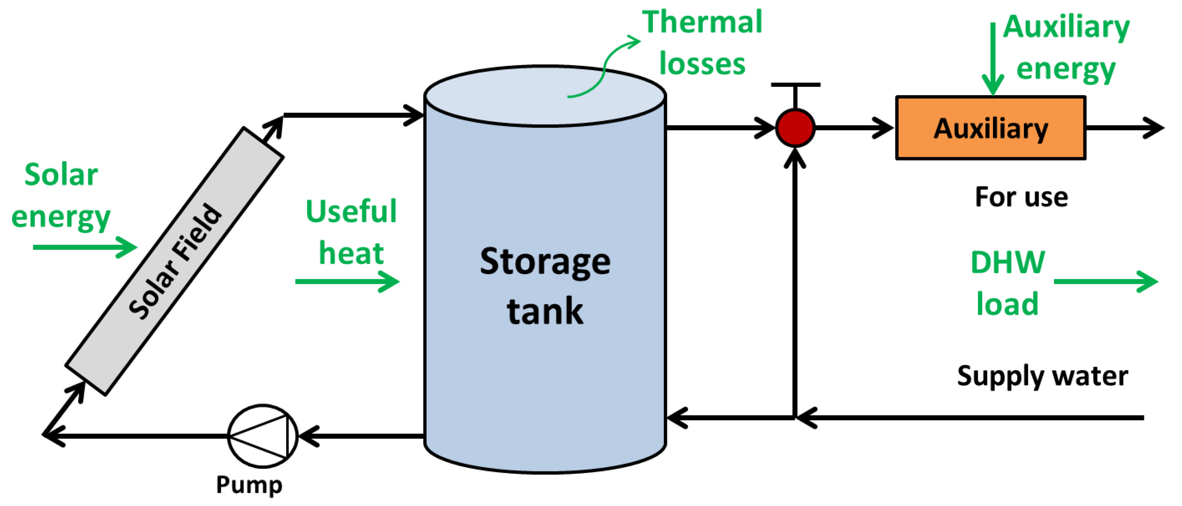
2.1. Overall Configuration

In this work, a solar thermal field coupled to a storage tank is examined in order to provide DHW for a building with 30 residents. There is an auxiliary system in this system that aids the system to warm up the water up to 45 °C when there is not enough solar potential. Moreover, the hot water from the tank is properly mixed with supply water from the grid when the tank has a temperature higher than the desired level of 45 °C. According to the Greek regulations (TOTEE-KENAK) [25], the specific energy demand per person is 50 L/day, so the total demand is selected to be 1500 L/day. Figure 1 shows briefly the examined system.

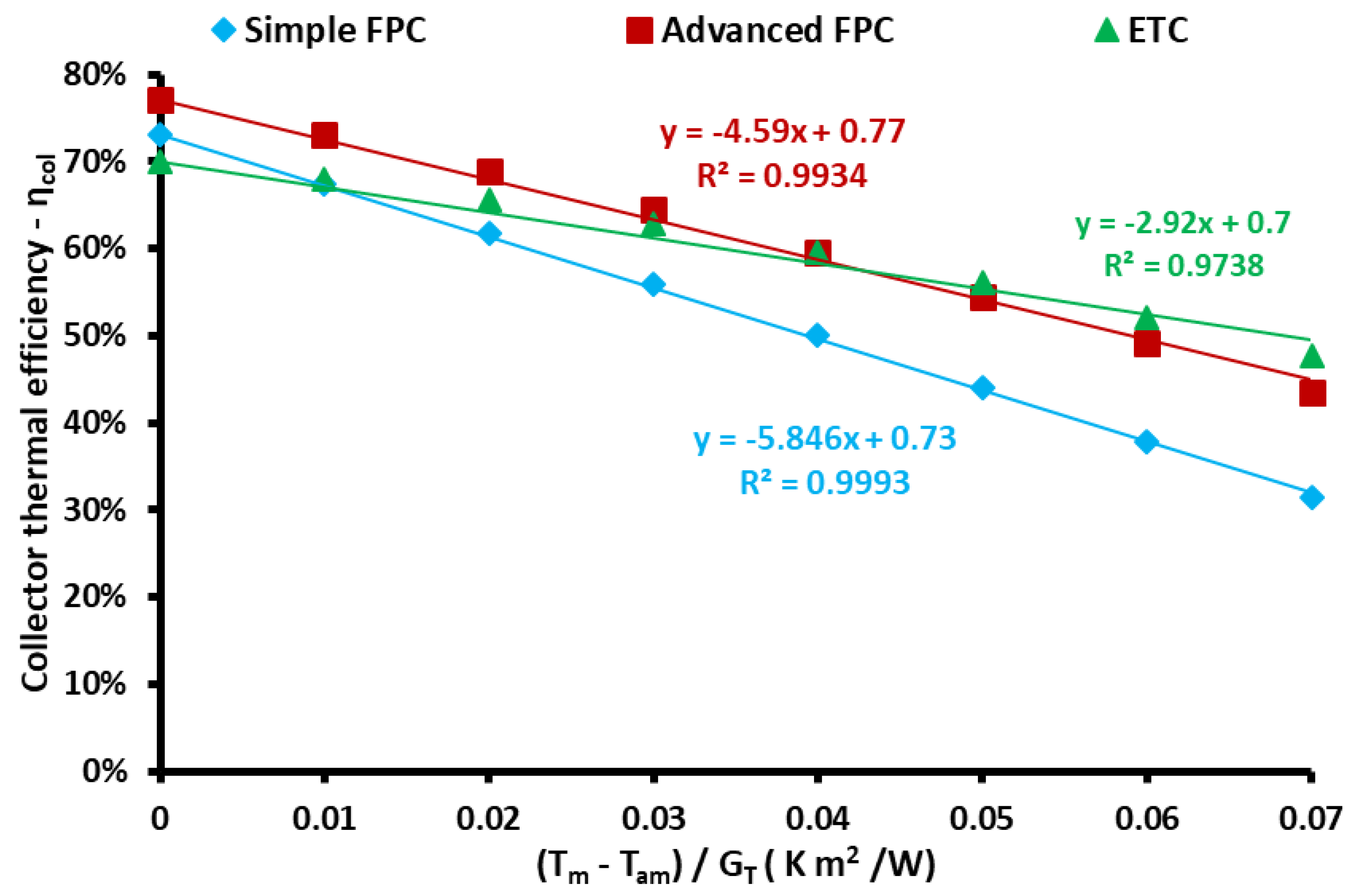
2.2. Solar Thermal Collectors

In this work, the solar thermal collectors are examined by using data for their performance according to the Greek legislation (TOTEE-KENAK) [25]. Three different solar thermal collectors are tested, and their thermal efficiency (ηcol) is described below:
η col = a 0 a 1 T fluid T am G T a 2 ( T fluid T am ) 2 G T
The coefficients (a0), (a1), and (a2) are the efficiency coefficients of the examined solar collectors which are given in Table 1 and they have been taken from Ref [25], while the parameter (GT) is the incident solar irradiation on the collector tilt surface. More specifically, this work investigates the simple flat plate collector (Simple FPC), the advanced selective flat plate collector (Advanced FPC), and the collector with evacuated tubes (ETC).
In this work, the followed methodology for the performance estimation of the integrated system is conducted by using the f-chart method, which is an acceptable and validated method [26]. This method needs the solar thermal collector efficiency to be estimated with a linear approximation following the next format [27]:
η col = F R ( τ α ) F R U L T fluid T am G T
where (FR) is the heat removal factor, (UL) is the total thermal loss coefficient, and (τα) is the product of cover transmittance and absorber absorbance. Following this methodological restriction, the efficiency curves of the different solar thermal collectors were converted into linear equations by conducting the proper approximations according to Figure 2. These results have been extracted for typical reference conditions (see References [25,27]) which are ambient temperature Tam = 25 °C and incident total solar irradiation GT = 1000 W/m2. It is obvious that the approximation coefficient R2 is very high for all the cases according to Figure 2, and so these approximations are assumed to be valid. Table 2 summarizes the coefficients [FRUL] and [FR(τα)], which were calculated from Figure 2 and will be used in the f-chart method. These two parameters are characteristic parameters of the solar thermal collectors, and they are assumed to be constant during the analysis.

2.3. The F-Chart Method

As it was previously said, the f-chart method [26,27,28] is a well-validated and acceptable method for the estimation of the solar fraction on the solar thermal units for DHW and space heating. This work regards a system that produces useful heat only for covering the DHW needs and also it includes an electrical heater as the auxiliary heat source.
In this method, there are two logistic parameters (X) and (Y) which lead to the calculation of the monthly solar fraction (f). These parameters are defined as below:
X = F R U L F R F R ( T ref T am , m ) Δ t A col L
Y = F R ( τ α ) n F R F R ( τ α ) ( τ α ) n H T N A col L
where (Acol) is the collecting area, (τα)n the thermal transmittance product at normal irradiation, (FR′/FR) the ratio of the ret removal factor of the system to the collector, (HT) the daily solar energy on the solar field area, (Δt) the total seconds of the month, (N) the number of the days in the month, (Tam,m) the mean ambient temperature of the month, (Tref) is the maximum system temperature chosen at 100 °C and (L) is the thermal load of the month for the DHW. In this work, the ratio (FR′/FR) is selected to be 0.95 as a typical value, while the ratio [(τα)/(τα)n] has a small monthly variation between 0.94 for winter and 0.90 for summer [26,27,28].
The use of the parameters (X) and (Y) makes possible the calculation of the monthly solar fraction (f) for the liquid systems by using the following formula [26,27,28]:
f = 1.029 Y 0.065 X 0.245 Y 2 + 0.0018 X 2 + 0.02 Y 3
It is critical to state that for the cases that f > 100% then it is selected at f = 100% in order to have reasonable results. Moreover, the storage tank of this work is selected to have a storage volume that is dependent on the collecting area according to the following expression [28]:
V   [ m 3 ] = 0.075 A c o l [ m 2 ]
The monthly solar fraction is practically the ratio of the energy that is exploited by the sun to the total load. Usually, this parameter is expressed in an indirect way by introducing the consumption from the auxiliary source (Laux) as below:
f = 1 L a u x L
The yearly solar coverage (F) is found by utilizing the monthly solar coverage (fi) and the monthly load (Li):
F = i = 1 12 f i L i i = 1 12 L i
In the present work, the thermal load is calculated as below:
L = ρ V w c p ( T hot T cold ) N
where (Vw) is the daily water need expressed in [m3], (N) are the days of the month, (Thot) is the desired temperature at 45 °C, (Tcold) is the temperature from the cold grid water equal to (Tcold = Tw,m), (ρ) is the water density and (cp) is the water-specific heat capacity. The cold temperature is calculated according to the Greek Technical Chamber data for every location separately [29].
The auxiliary energy (Laux) can be expressed as below:
L aux = ( 1 f ) L
The energy that provides the solar thermal system for covering the load (Lu,sol) can be found below:
L u , sol = f L

2.4. Economic Evaluation
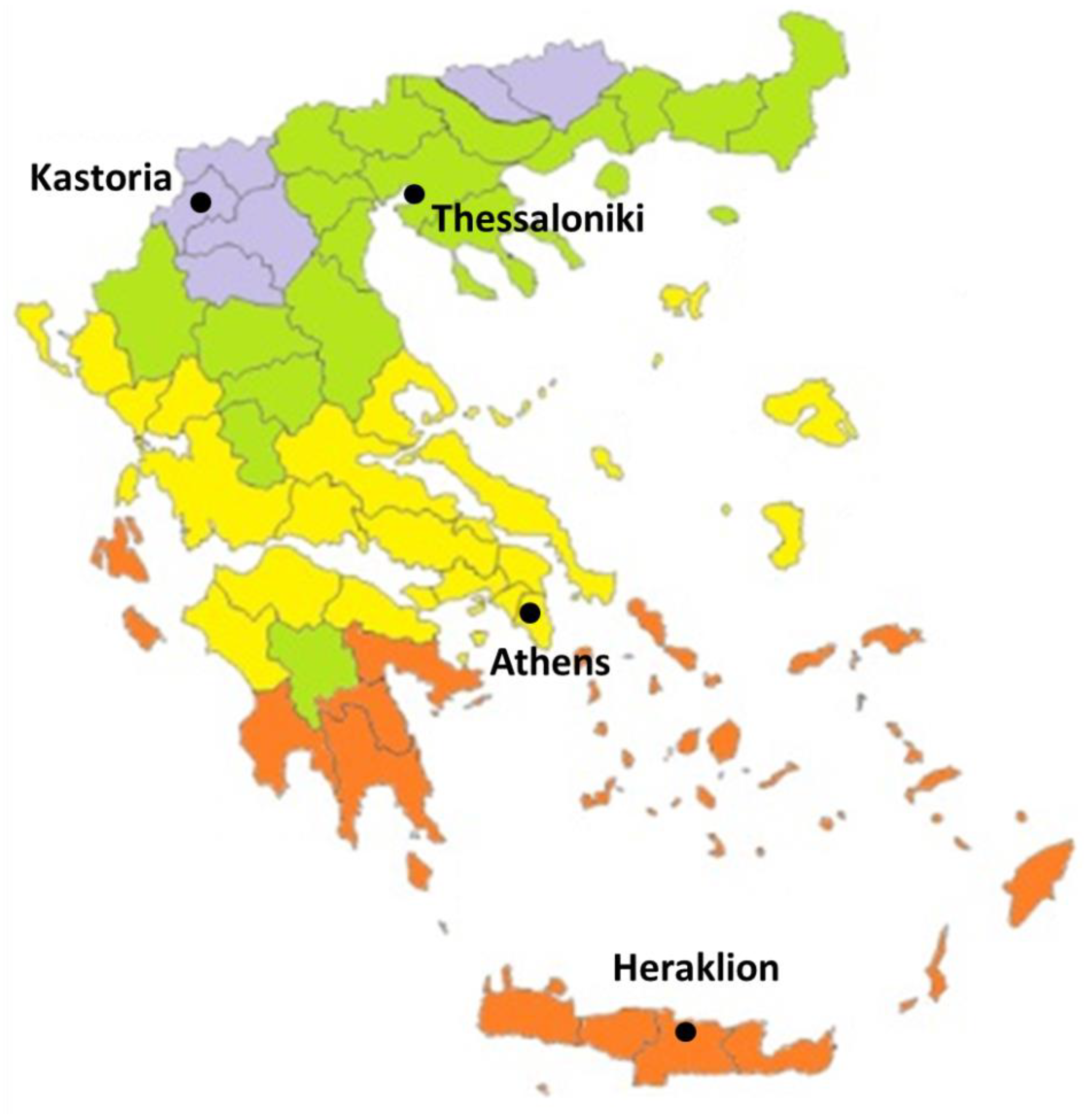
The present study includes also an economic evaluation of the examined units. The capital cost of the unit can be found according to the next equation:
C 0 = K col A col + K tank V tank
The tank specific cost (Ktank) is selected at 1000 €/m3 [30,31], while the specific cost of the collectors (Kcol) is chosen at 120 €/m2 for the Simple FPC, at 150 €/m2 for the Advanced FPC, and at 250 €/m2 for the ETC [30,31].
In this work, the discount factor (r) is assumed to be 5%, the project lifetime (M) at 25 years, and the electricity cost (Kel) for the auxiliary source at 0.20 €/kWh. The yearly economic gain by the use of the solar system is calculated as below:
CF gain = K el L u , sol
Practically, this gain indicates the money that would have been spent on the auxiliary system operation for covering the demand if there was not the solar system.
The first introduced parameter for the economic analysis is the simple payback period (SPP) which is calculated as the ratio of the capital cost of the investment to the yearly economic gain by the use of the solar system:
SPP = C 0 CF gain .
The next financial index is the life cycle cost (LCC) of the unit which takes into consideration the total money that will be spent for covering the DHW demand for all the project life.
LCC = C 0 + i = 1 M L aux K el ( 1 + r ) i
The goal is the minimization of both the (SPP) and the (LCC) in order to achieve optimal economic behavior. The (LCC) is assumed to be a better index than (SPP) because it takes into consideration all the life of the project and it is able to indicate future gains after the payback period. On the other hand, the (SPP) is a usual index in order to evaluate quickly investment with relatively low capital cost. Both indexes are important and thus these are both included in the present work.

2.5. Weather Data

In this work, the provided weather data from Greek Technical Chamber [29] are used in order to estimate the daily solar energy on the tilted surface (HT). More specifically, the global irradiation on the horizontal surface (H) and the diffuse irradiation on the horizontal surface (Hd) are properly combined in order to find the (HT). These data regard the mean monthly day for four different Greek cities. Every city is a representative one for every different climate zone. Table 3 gives the data about the (H) and Table 4 the data about the (Hd) for the studied locations. Moreover, the yearly solar irradiation values are summarized in the previous tables. The data have been taken from Ref. [29].
Figure 3 depicts the examined cities and the respective climate zone separation in Greece. More specifically, in the work Zone A is examined with the city of Heraklion (35°20′ N, 25°8′ E), Zone B with the city of Athens (37°59′ N, 23°43′ E), Zone C with the city of Thessaloniki (40°37′ N, 22°56′ E) and Zone D with the city of Kastoria (40°31′ N, 21°16′ E).
The next step in this work is the calculation of the solar energy that receives the tilted surface (HT). This calculation is possible by following the methodology of the isotropic atmosphere proposed by Liu and Jordan [33] and extended by Klein [34].
H = R b ( H H d ) + ( 1 + cos ( β ) 2 ) H d + ρ g ( 1 cos ( β ) 2 ) H
where (ρg) is the reflectance of the ground equal to 0.2 [27], (β) the collector tile angle, and (Rb) the ratio of the beam irradiation on the tilted surface to the horizontal surface on the monthly base.
The parameter (Rb) is calculated according to the suggested methodology in Ref. [27]. For surfaces in the northern hemisphere with zero azimuth (facing the south), it can be written:
R b = cos ( φ β ) cos ( δ ) sin ( ω s ) + ( π 180 ) ω s sin ( φ β ) sin ( δ ) cos ( φ ) cos ( δ ) sin ( ω s ) + ( π 180 ) ω s sin ( φ ) sin ( δ )
The parameter ( ω s ) is the sunset hour angle for the collectors and it is calculated as below:
ω s = m i n [ cos 1 ( tan ( φ ) tan ( δ ) ) cos 1 ( tan ( φ β ) tan ( δ ) ) ]
where (φ) is the geographical latitude of the examined city and (δ) is the declination angle of the mean monthly day. More details about the calculation of the declination angle can be found in Ref. [27]. Table 5 gives the results of the solar energy on the tilted surface for different angles and locations.
The next step regards the temperature levels of the air and the water. The mean monthly temperature (Tam,m) and the mean monthly water temperature from the grid (Tw,m) are the temperature levels that are needed for all the months and all the studied locations. Table 6 includes all the data provided by Ref. [29].

2.6. Followed Methodology

The present investigation studies the DHW production by a solar thermal system with various collector types in the four different climate zones of Greece. For every climate zone, a representative city is selected to be studied. The f-chart method [26,27,28] is selected to be used and the weather data have been taken from the Greek Technical Chamber [29]. The analysis is energetic and economical by examining two main parameters. The studied case regards a building with 30 residents with a daily demand of 1500 L (=1.5 m3) at 45 °C. The collecting area is examined from 5 m2 up to 40 m2, while the tilt angle is from 30° up to 50°. The storage tank volume follows the solar is by assuming 75 L every 1 m2. Critical parameters of the analysis are the solar coverage (f) on the monthly basis, the solar coverage (F) on the yearly basis, the simple payback period (SPP), and the life cycle cost (LCC) of the investment.
More specifically, the first part of this work includes a detailed parametric investigation in order to show the influence of the collecting area (Acol) and of the tilt angle (β) on the unit’s energy performance. The next stage is the optimization of the unit according to the criterion of the (LCC) minimization. The last part of this work is a multi-objective evaluation of the different designs based on the solar coverage (F) and the (SPP) criteria. The aforementioned methodology makes possible an overall view of the system behavior with energy and economic criteria in order to extract valuable conclusions for the future designs of the solar thermal unit for DHW in Greece.
Last but not least, it is important to briefly describe the methodology of the multi-objective optimization study. For every location, all the points of the collecting areas and the collector types are the possible optimum design cases. All these are evaluated in order to determine the final optimum choice according to the energy and economic criteria. The solar coverage and the SPP are the selected criteria in this optimization analysis. The ideal of the followed analysis is to determine the design point that is closer to the ideal one. The ideal point is the one with the minimum SPP and the maximum (F). However, it is an ideal one and not a real design point. The dimensionless geometrical distance (DD) is calculated for every point and the point with the minimum (DD) is the overall optimum case. The use of the dimensionless and not the real geometric distance is something important in order to take into account both criteria in the same way. More specifically, it can be written [35]:
D D = ( S P P S P P m i n S P P m a x S P P m i n ) 2 + ( F m a x F F m a x F m i n ) 2
where the subscripts “min” and “max” correspond to the minimum and the maximum obtained values among the examined designs.
It is useful to state that for every location, 8 different collecting areas for every collector type are evaluated, so 24 different design scenarios are used in every multi-objective optimization analysis. The optimum tilt angles are used in the analysis. Totally, this procedure is performed four times; one for every climate zone.

3. Results and Discussion

The results of the present investigation are given in this section. More specifically, the results regard the economic and energy evaluation of the system. The influence of various parameters on the results is given, as well as the optimization of the system is presented.

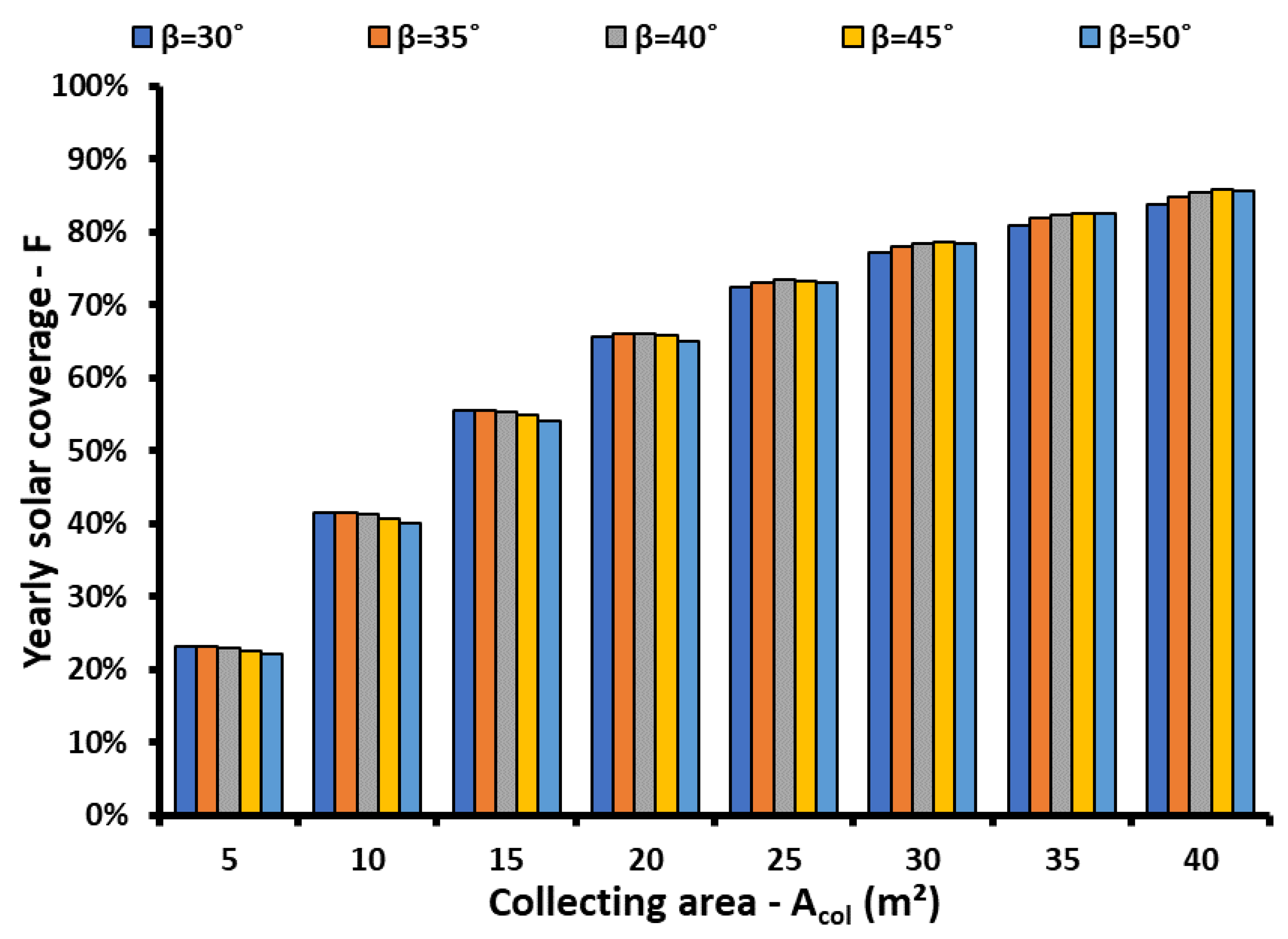
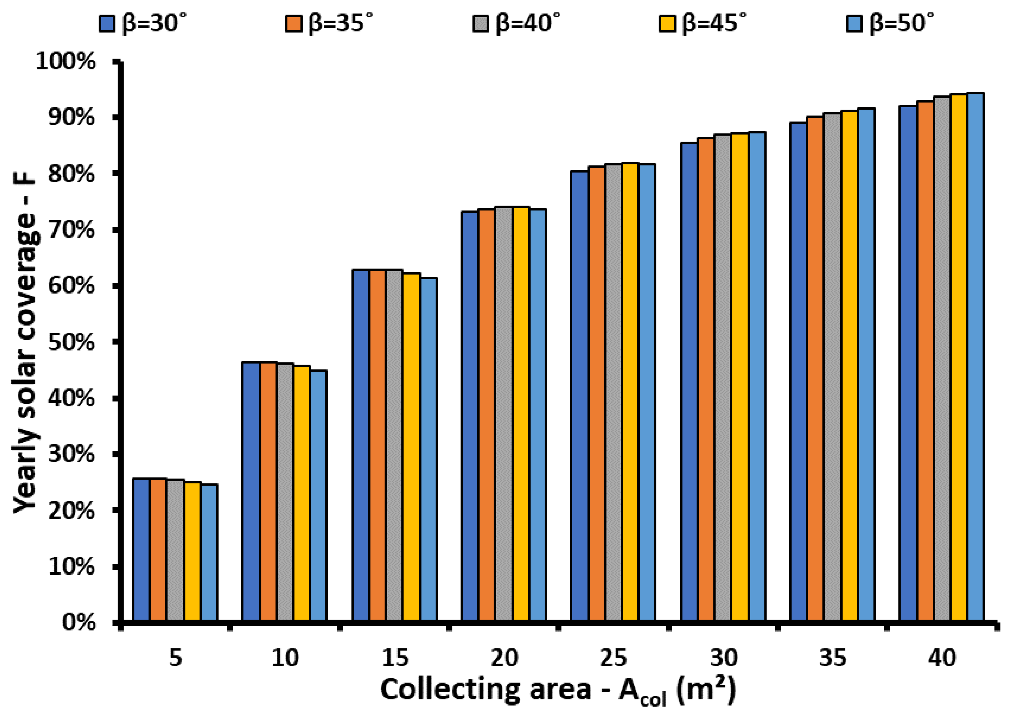
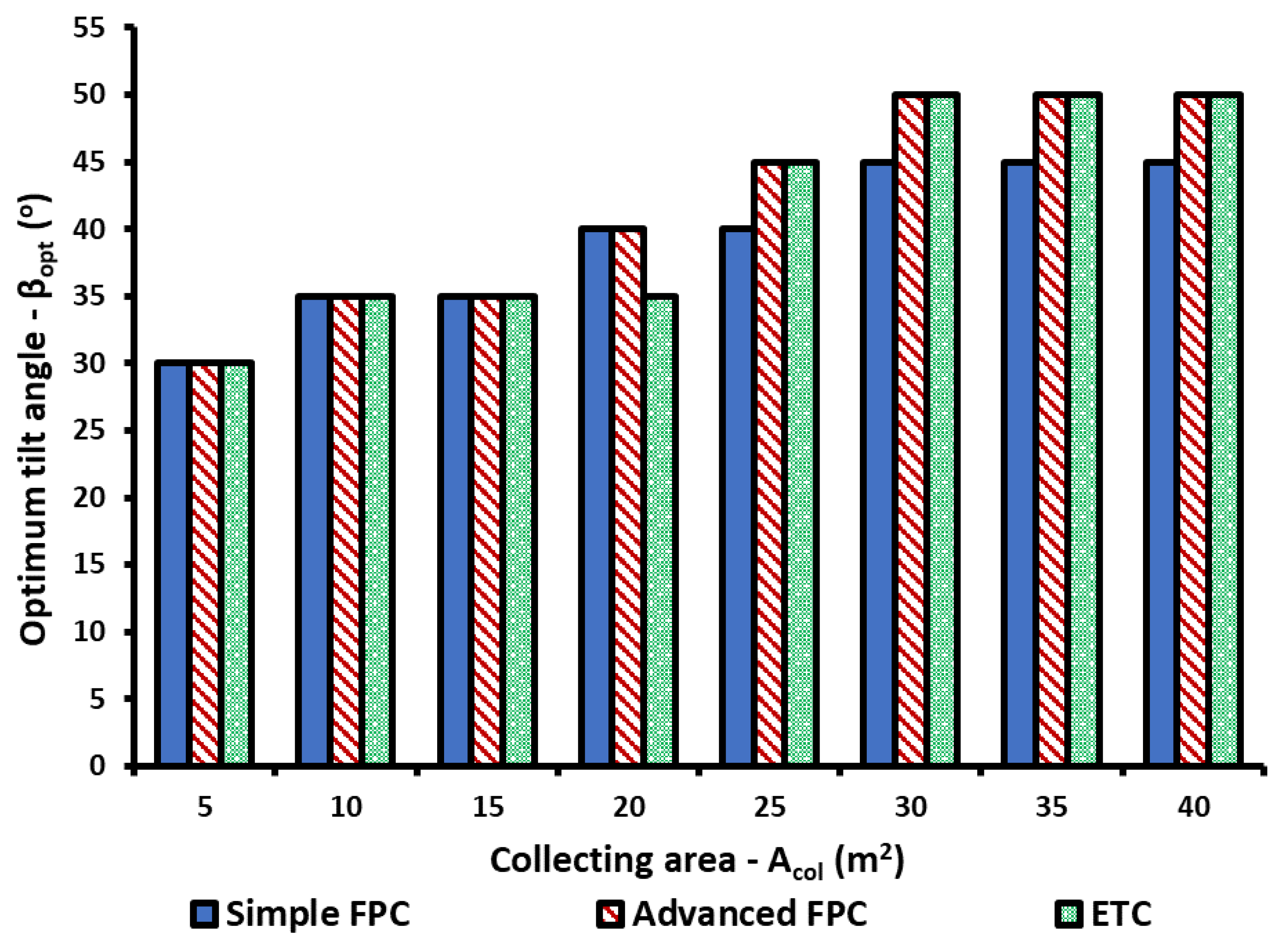
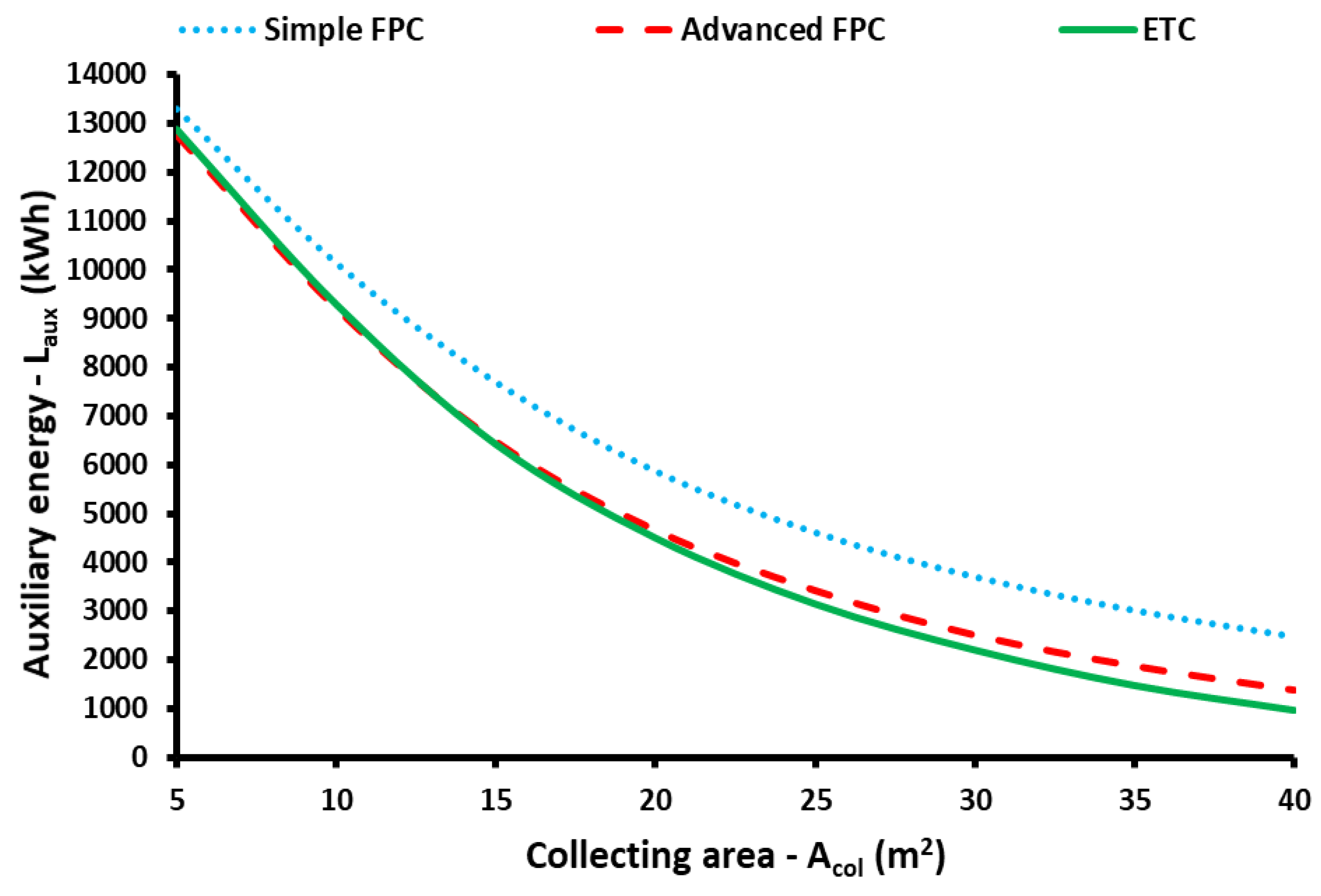
3.1. Parametric Analysis for the Climate Zone B—Athens

The first part of the parametric analysis regards the presentation of the basic impact of the collecting area and of the tilt angle on the results. The location of Athens (climate zone B) is selected to be used as the example city in order to present this initial parametric analysis. Figure 4 includes the results about the influence of the solar field area (Acol) on the yearly solar coverage (F) for different tilt angles (β) for Athens and for the simple FPC. Figure 5 is the respective depiction for the advanced FPC, while Figure 6 is the respective depiction for the ETC. These three figures lead to similar quality conclusions, which indicate that a higher collecting area increases the solar coverage, while the impact of the tilt angle is not so important to the results. However, among the examined cases, different optimum tilt angles can be found, something that indicates this parameter is an important one.
Figure 4 shows that for low collecting areas, the optimum tilt angle is at 30°, while for higher collecting areas the optimum value increases, and for the collecting area of 40 m2, it is at 45°. This is an interesting result that is based on the impact of the tilt angle on the seasonal available solar energy on the collector aperture. More specifically, in low collecting areas, the small tilt angles boost a lot during the summer period when there is great solar potential. However, in high collecting areas, the summer load is covered with all the tilt angles, thus the optimum tilt angle is the one that maximizes the winter performance. In other words, the conclusion that is obtained is that when there is a great collecting area, the angle has to be the best one for the winter period. Similar conclusions are obtained in Figure 5 and Figure 6. More specifically, the advanced FPC and the ETC are more efficient collectors compared to the simple FPC, something that makes possible the optimum tilt angle to be at 50° during the winter. At this point, it is useful to take into account that the higher tilt angle aids the winter operation because the sun has a lower height during the winter, and so the high tilt angle makes the solar rays more vertical during the winter. Also, please take into account that according to Ref. [27], the optimum winter angle for Athens can be 15° plus the geographical latitude, so to be 53°. Therefore, the values of 45–50° are acceptable.
Figure 7 summarizes the optimum tilt angles for different collecting areas and collector types for the location of Athens. Generally, the optimum tilt angles are similar for all the collector types. However, it can be said that in higher collecting areas, the more efficient collectors have to be placed with a bit greater tilt angle. Moreover, another conclusion is that the higher collecting leads to a higher optimum tilt angle in order to boost the winter because in the summer there is high coverage for all the examined tilt angles due to the plenty of areas.
Figure 8 shows the yearly solar coverage for the optimized cases for the location of Athens, while Figure 9 depicts the respective results for the auxiliary energy consumption by the electrical heater. Figure 8 and Figure 9 make clear that a higher collecting area makes the solar coverage higher, while the auxiliary consumption is lower. The increase of the solar coverage has a decreasing rate because, after the limit of 15 m2, it is not possible to utilize all the useful heat from the extra collecting area. The simple FPC presents significantly lower performance and thus lower solar coverage. The other collectors, advanced FPC and ETC, present similar performance with the advanced FPC to have an extremely higher performance in small collecting areas, while in great collecting areas the ETC is the best choice with a small but existing difference. The respective results are obtained for the auxiliary energy consumption, with the simple FPC leading to the higher consumption, while the other two collectors to similar values.

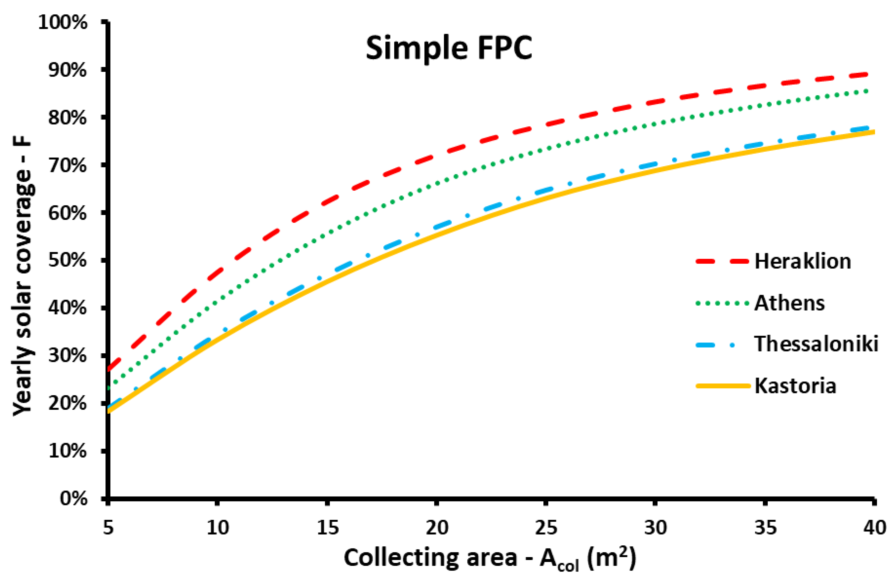
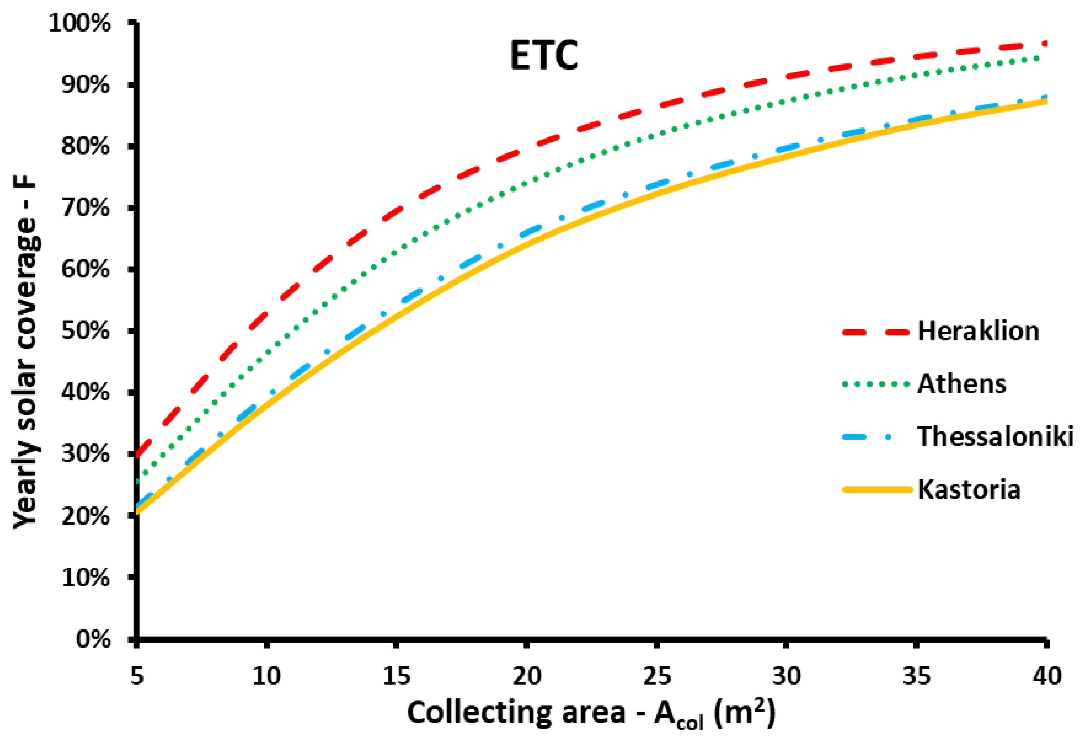
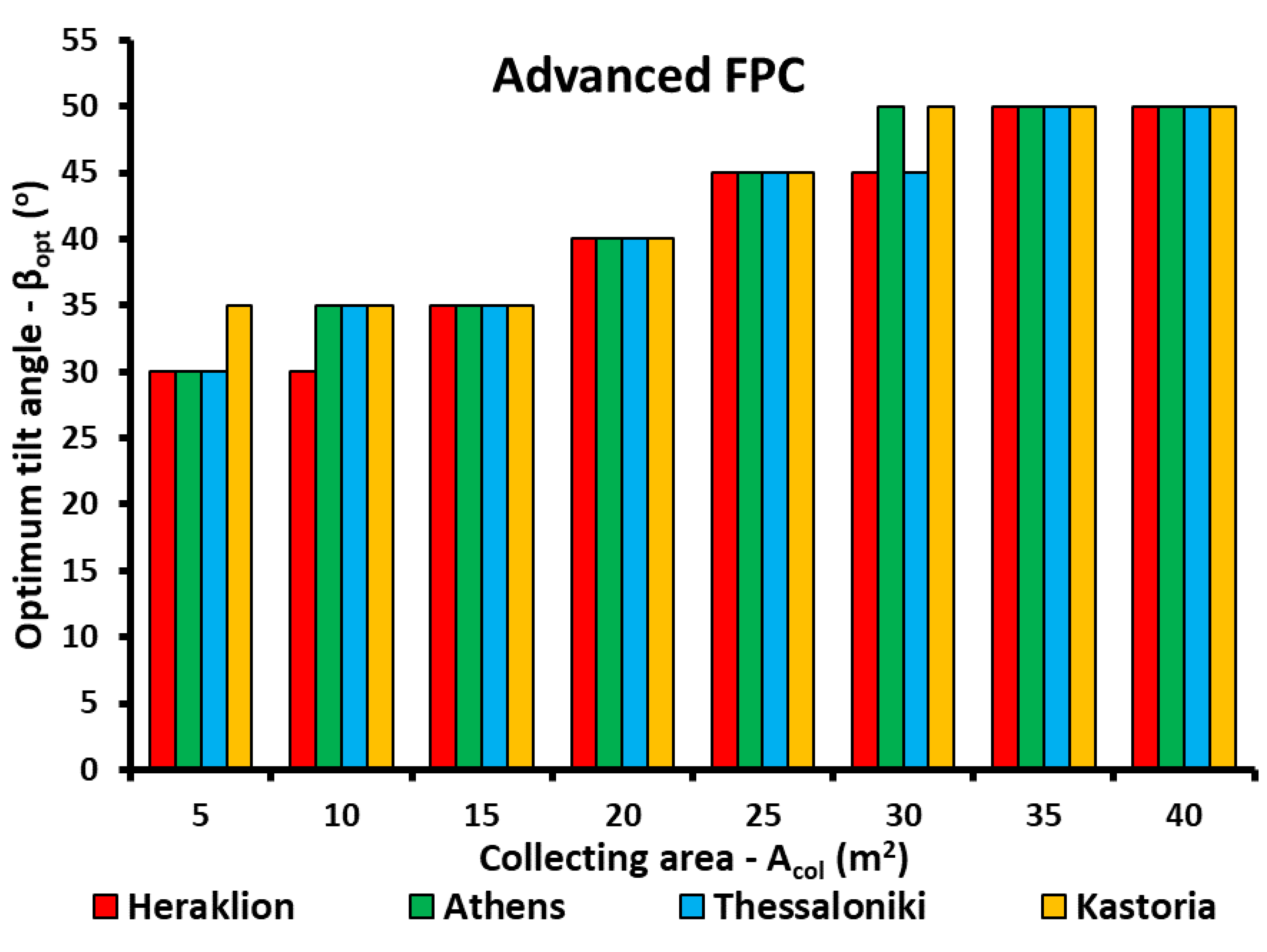
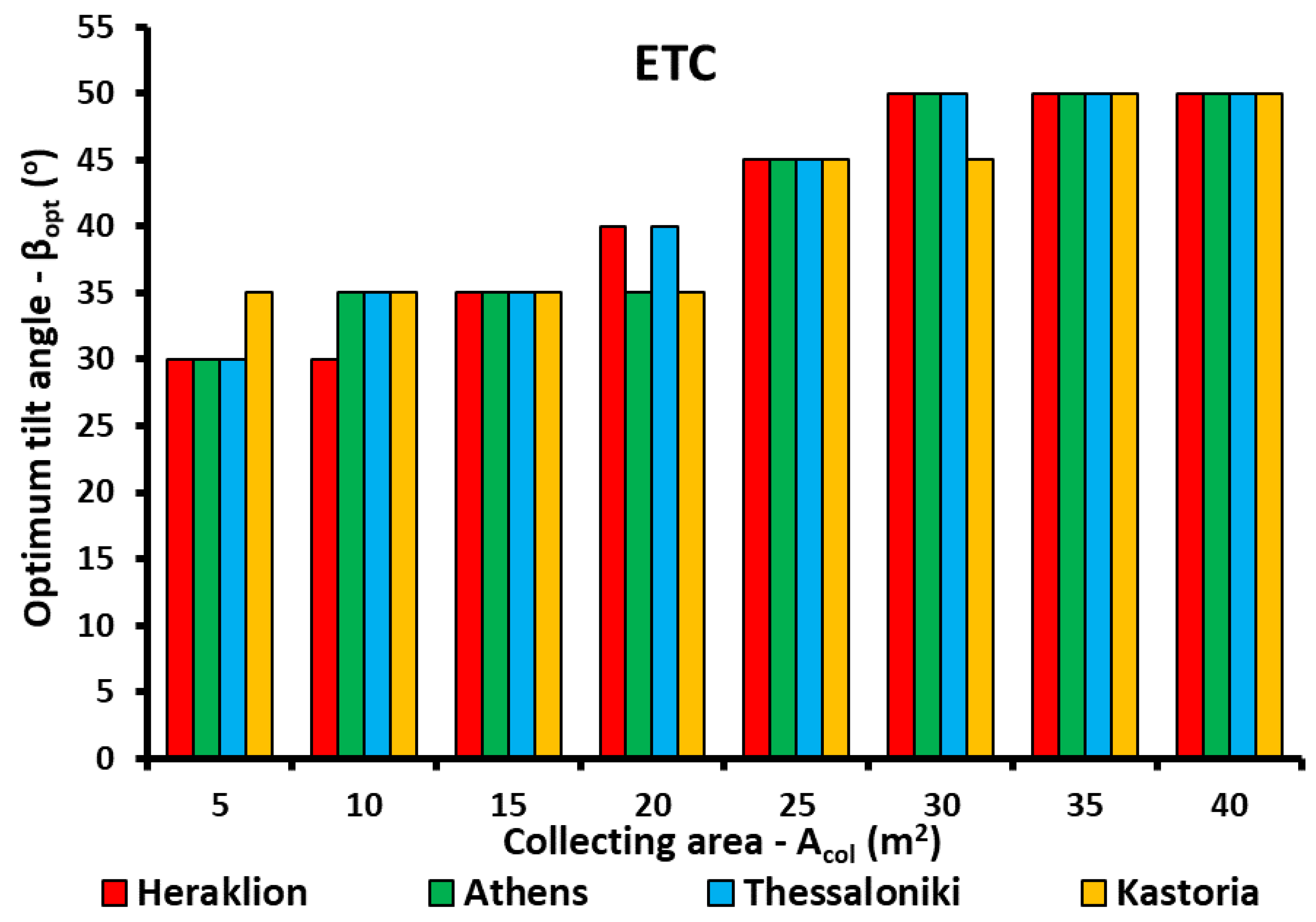
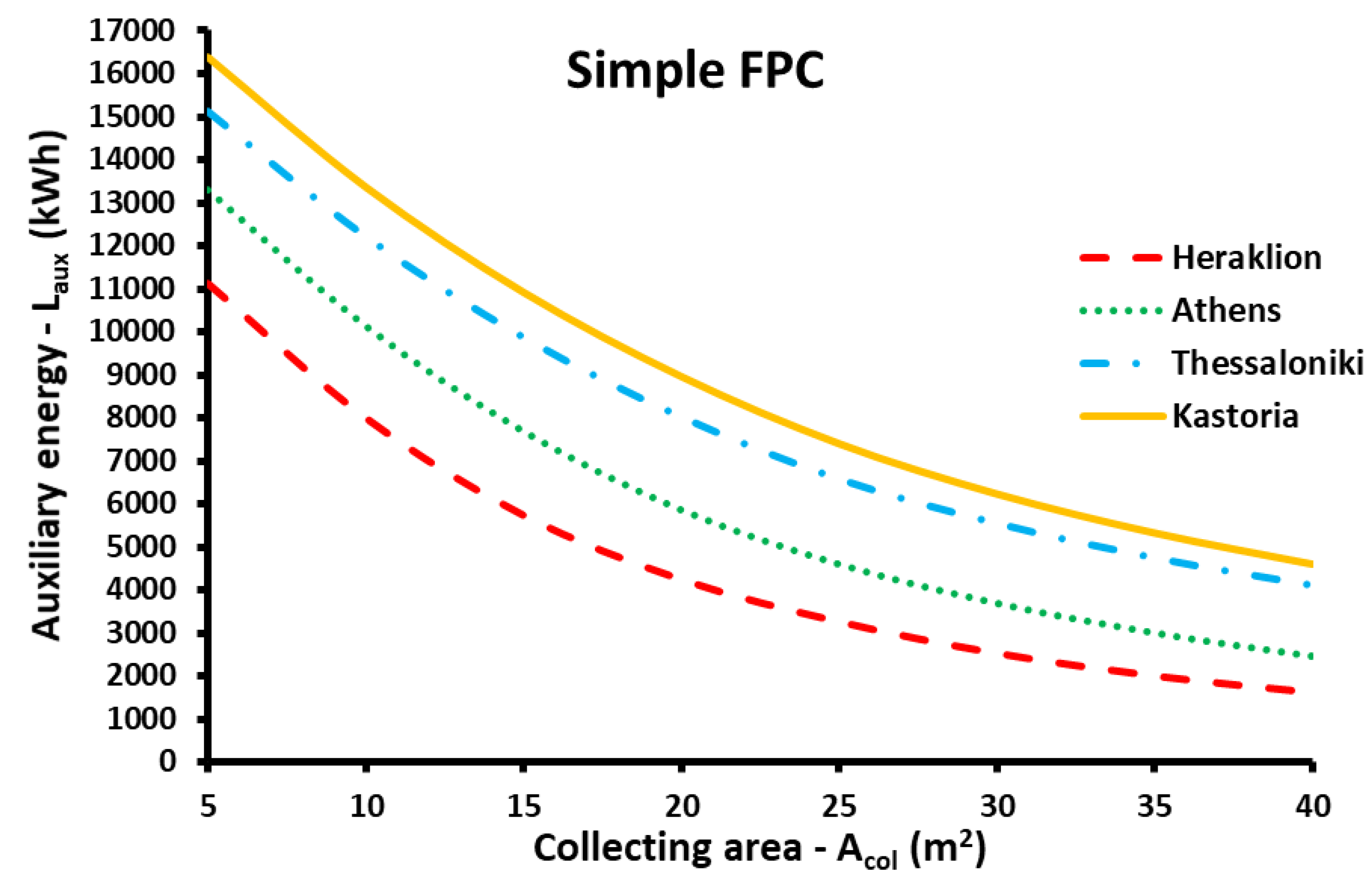
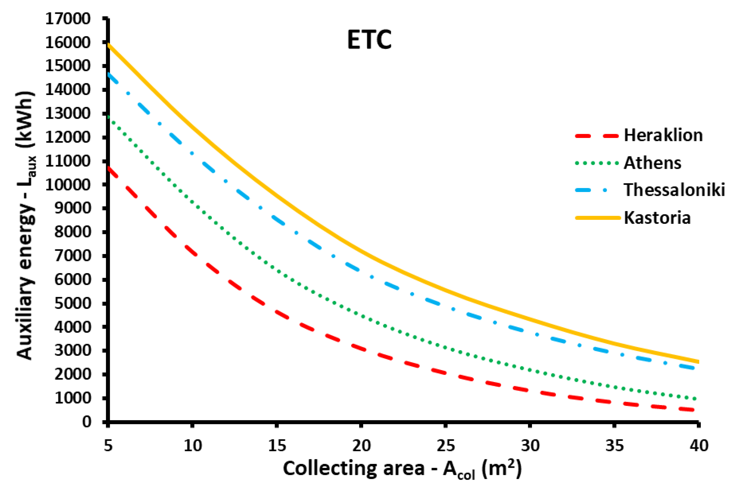
3.2. Comparison of the Energy Performance for Different Climate Zones

After the initial parametric analysis for Athens (Zone B), the results of the four climate zones are presented in Section 3.2. It is notable to state that the yearly demand for useful heat for the building is 15,295 kWh for Heraklion, 17,301 for Athens, 18,687 kWh for Thessaloniki, and 20,037 for Kastoria. These values are depended on the water temperature from the grid because the colder climate zones have lower water temperatures, and so higher energy amounts are needed for warming the water up to the desired temperature level. Figure 10, Figure 11 and Figure 12 show the yearly solar coverage for the simple FPC, the advanced FPC, and the ETC, respectively. These results concern the operation with the optimum tilt angle in every case which maximizes the yearly solar coverage. According to the results for Figure 10, Figure 11 and Figure 12, the solar coverage is higher for Heraklion with Athens, Thessaloniki, and Kastoria to follow, respectively. These results are reasonable because the solar coverage is higher in warmer locations with higher potential and higher temperatures. It is critical to state that the difference between Thessaloniki and Kastoria is very small for all the collector types. At this point, it is important to state that for Heraklion, the maximum solar coverage is found at 96.75%, for Athens at 94.45%, for Thessaloniki at 87.98%, and for Kastoria at 87.41%; all these maximum values for 40 m2 collecting area and ETC.
The next presented results regard the values of the optimum angles for all the locations and the collector types. Figure 13 shows the optimum angles with the simple FPC, Figure 14 with the advanced FPC, and Figure 15 with ETC. The general result is that a greater collecting area leads to a higher optimum tilt angle. Moreover, for the same collector type and collecting area, the optimum tilt angle is similar for the various locations, with small deviations of 5° in some cases.
The last step concerns the results of the auxiliary energy consumption on the yearly basis for the different cases with the optimized tilt angle. It is important to state that the maximization of the yearly solar coverage leads to the minimization of the yearly auxiliary energy consumption by the electrical heater. Figure 16, Figure 17 and Figure 18 show the results of the auxiliary energy consumption of the simple FPC, the advanced FPC, and the ETC, respectively. For all the collector types, the lowest auxiliary energy consumption is found for Heraklion, with Athens, Thessaloniki, and Kastoria to follow. For the case with ETC and 40 m2, the lowest consumptions are found at 497, 961, 2245, and 2522 kWh for Heraklion, Athens, Thessaloniki, and Kastoria, respectively.
Kastoria has the greatest consumption and there is a notable difference with Thessaloniki, while the respective difference in the solar coverage was very small. This result can be explained by the different needs among the locations, so it is obvious that the results about solar coverage and auxiliary energy consumption have the same trends but there are small deviations regarding the distance between the curves. In any case, the final conclusions indicate that the auxiliary energy consumption is lower in the warmer climate zones.

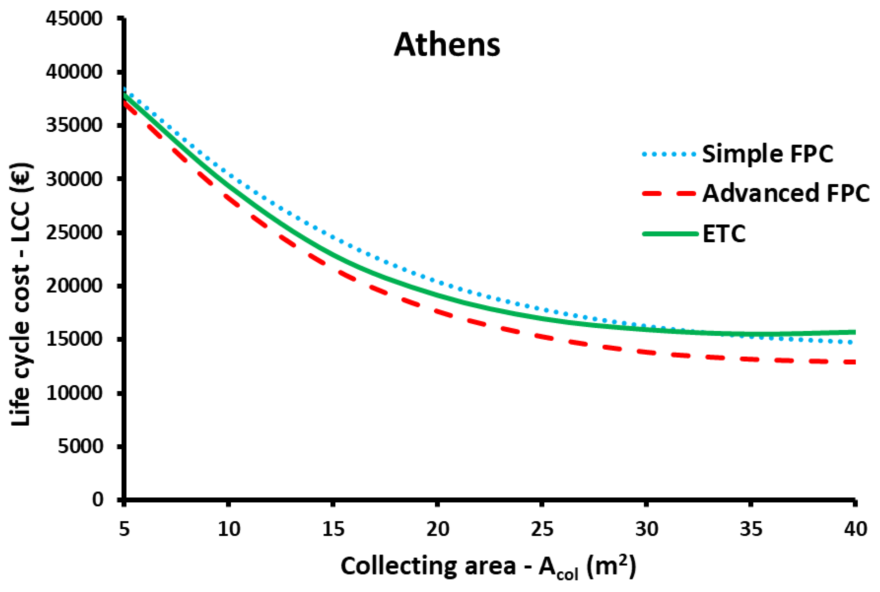
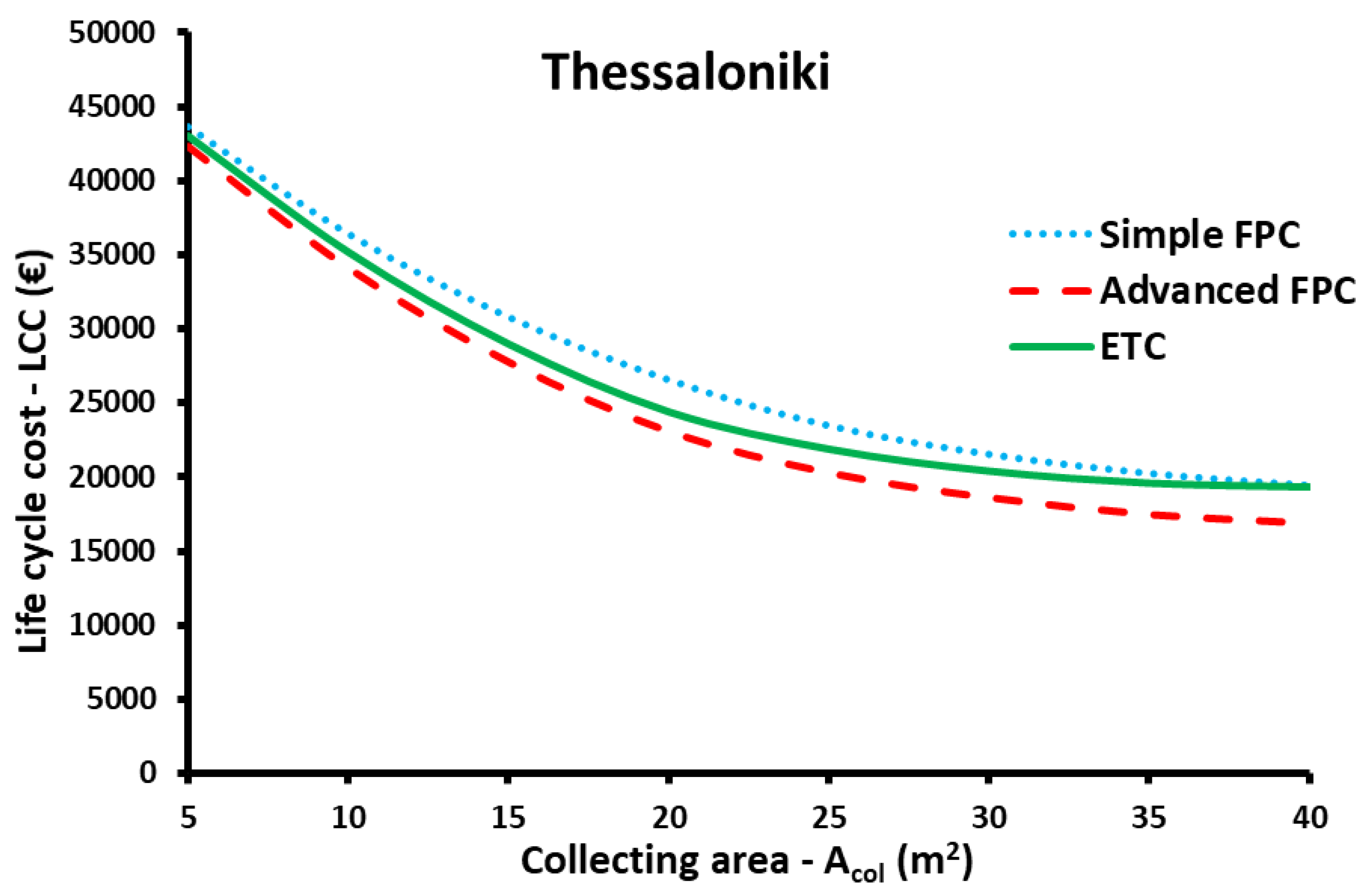
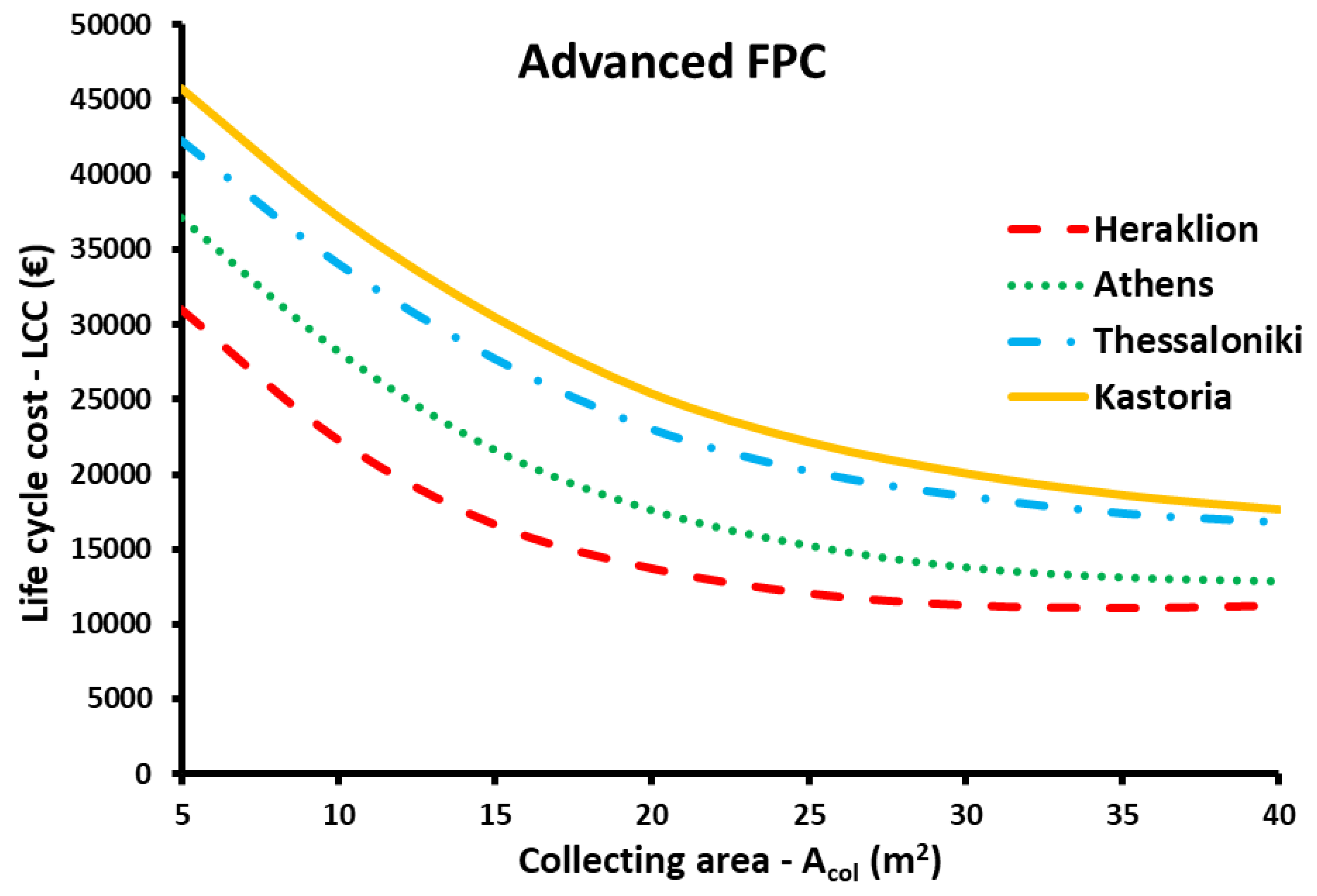
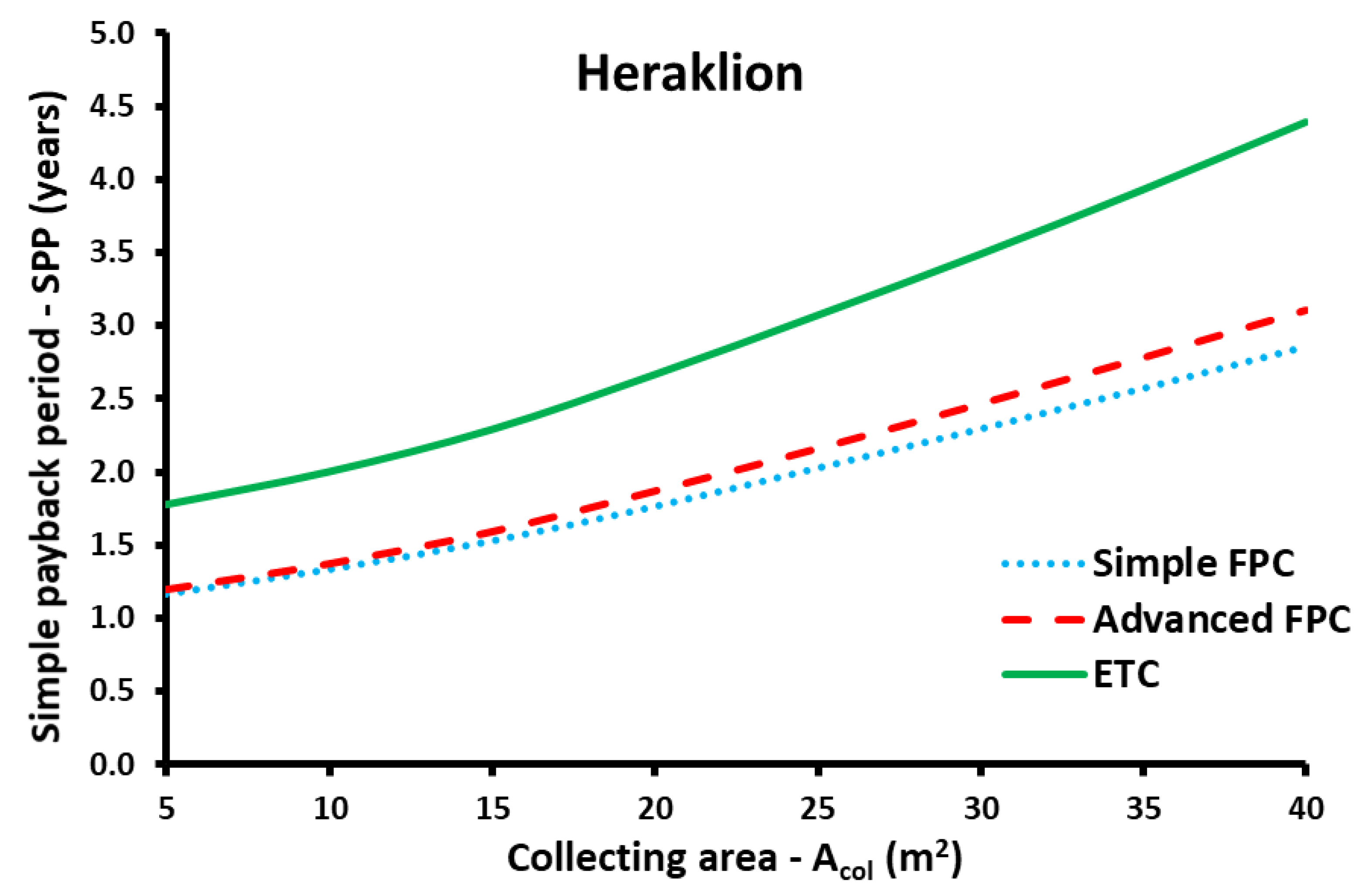
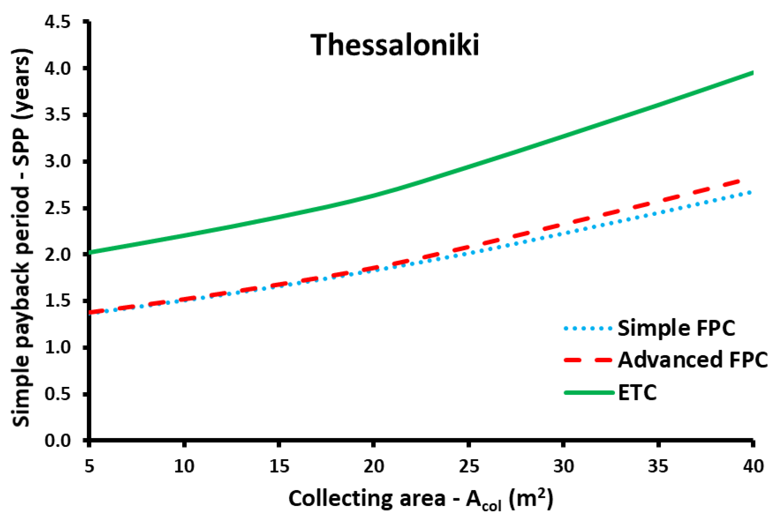
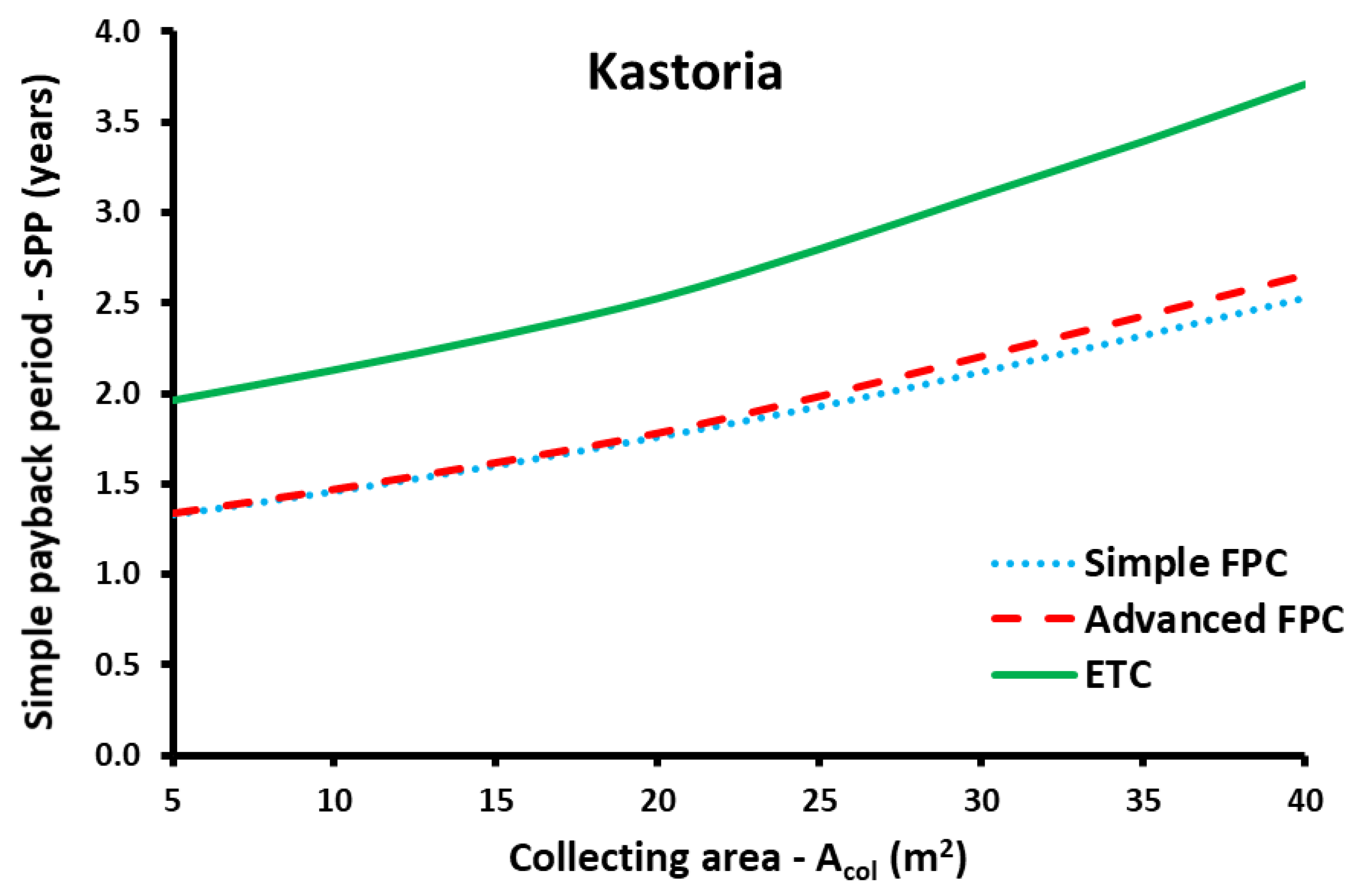
3.3. Economic Optimization

The economic analysis of this work is conducted only for the cases with optimum tilt angles because in these cases, the solar coverage is maximized, and the auxiliary energy consumption is minimized. So, the operational cost of the system is minimized. Moreover, the placement of the solar collectors at different angles does not lead to different costs, thus there is not any reason to take into account all the tilt angles in the economic analysis. Practically, the optimum economic choices would be for cases with optimum title angles. Therefore, the examined parameters in the economic analysis are the collecting area and the collector type.
Figure 19, Figure 20, Figure 21 and Figure 22 show the results of the life cycle cost (LCC) of the unit for the cities of Heraklion, Athens, Thessaloniki, and Kastoria, respectively. The general image of these figures indicates that the increase of the area leads generally to lower LCC and in some cases, it is minimized for collecting areas in the range of 30 to 40 m2. Moreover, the most important conclusion from the LCC analysis is that the advanced FPC is the best choice for all the locations. This result is a very interesting one because it indicates the selection of the advanced FPC for all the possible examined cases. This is an efficient collector with an acceptable cost and thus the economic evaluation makes it the most appropriate choice.
Table 7 includes the results for the optimal operation according to the LCC criterion and more specifically, the best design for every collector type is given. For the Heraklion, the minimum LCC is 11,088 € for the 35 m2 of advanced FPC, with the 40 m2 of simple FPC to follow at 12,383 € and the less viable choice is the 30 m2 of ETC with 13,480 €. For Athens, the minimum LCC is 12,875 € for advanced FPC and 40 m2, with the 40 m2 of simple FPC to follow at 14,737 € and the last choice is the 35 m2 of ETC with 15,518 €. For Thessaloniki, the minimum LCC is found for advanced FPC at 16855 € for 40 m2, with ETC to follow at 19,329 € at 40 m2 and simple FPC at 19,405 € at 40 m2. For Kastoria, the advanced FPC leads to the minimum LCC at 17,692 € with 40 m2, with 40 m2 ETC to follow at 20,110 € and 40 m2 simple FPC to follow at 20,784 €. It is obvious that the advanced FPC is the best solar technology for all the locations. For this reason, Figure 23 shows the LCC for the four locations with this collector. It is concluded that the lower LCC is found for Heraklion, with Athens, Thessaloniki, and Kastoria to follow, respectively.
Figure 24, Figure 25, Figure 26 and Figure 27 depict the results of the simple payback period (SPP) of the unit for the cities of Heraklion, Athens, Thessaloniki, and Kastoria, respectively. Moreover, Table 7 gives the results for the SPP for the cases with minimum LCC. The SPP, for all the locations and collector types, has an increasing rate with the increase of the collecting area. Moreover, the minimum SPP is found for the simple FPC. These results make clear that the overall minimum SPP is found for the cheapest choice with a 5 m2 simple FPC. However, these designs are not acceptable according to energy analysis because the solar coverage is low in these cases. Therefore, a multi-objective optimization study is presented in the next subsection in order to take into consideration both the SPP minimization and the yearly solar coverage maximization.
Another interesting conclusion is that the SPP takes relatively low values in all the cases. More specifically, the SPP is lower than 4.5 years in all the cases; a valuable result that clearly shows that the investment in solar thermal systems is a viable one. The high electricity price, which is considered at 0.20 €/kWh in this work, is the main reason for the low SPP values. Therefore, this study comes to prove, in a clear and accurate way, that the recent increases in electricity prices make the exploitation of solar energy vital for the sustainability and viability of future energy systems.
Taking into account the optimal choices according to the LCC minimization criterion (see Table 7), the SSP for Heraklion is 2.85, 2.78, and 3.49 years for the simple FPC, the advanced FPC, and the ETC, respectively. For the same collector type sequence, the SPP is 2.63, 2.83, and 3.59 years, respectively, for Athens, 2.68, 2.83, and 3.95 years, respectively, for Thessaloniki, while 2.53, 2.65, and 3.71 years, respectively, for Kastoria. The conclusion is that the ETC leads to higher SPP due to the higher investment cost compared to the other collectors.

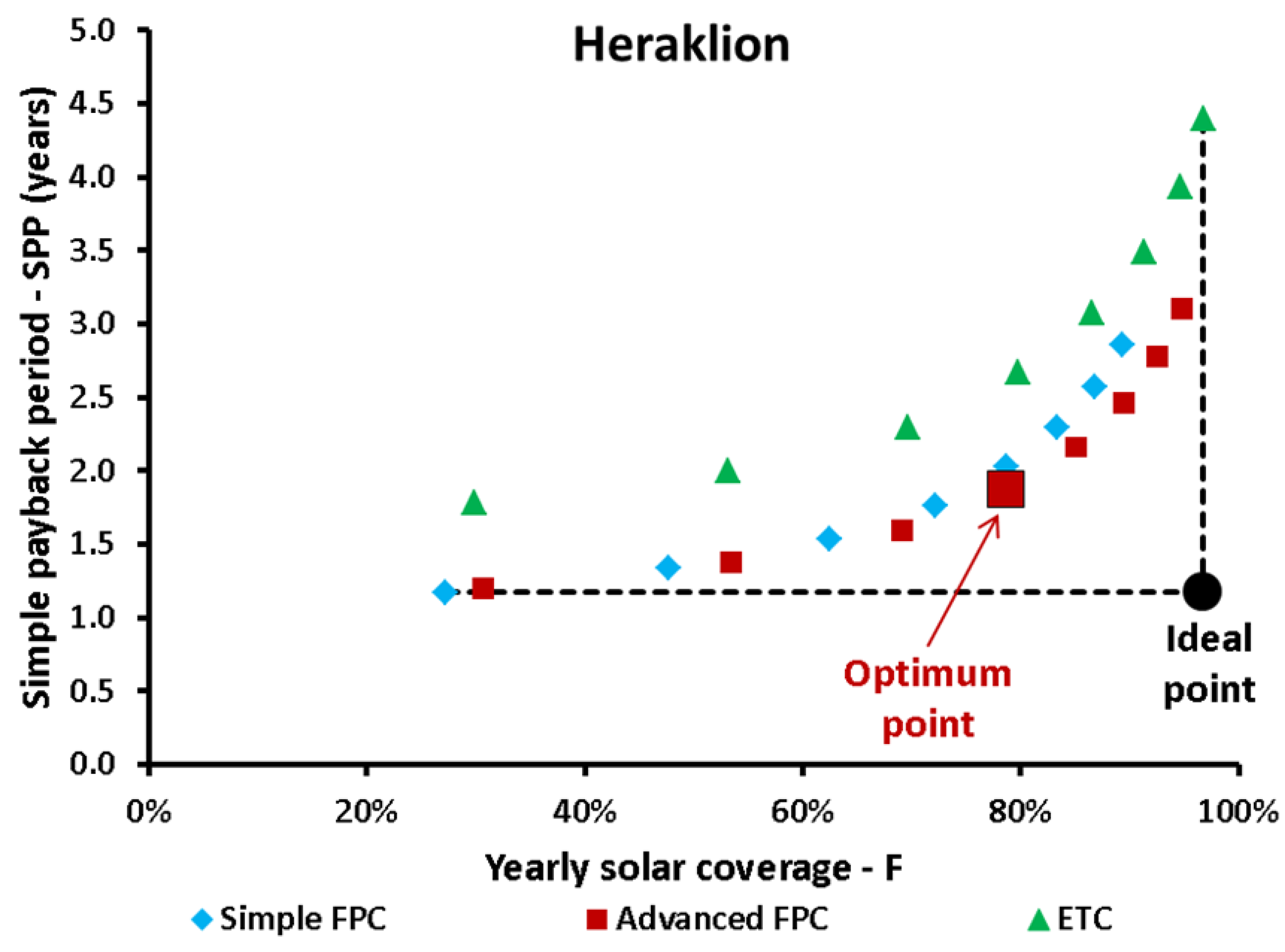
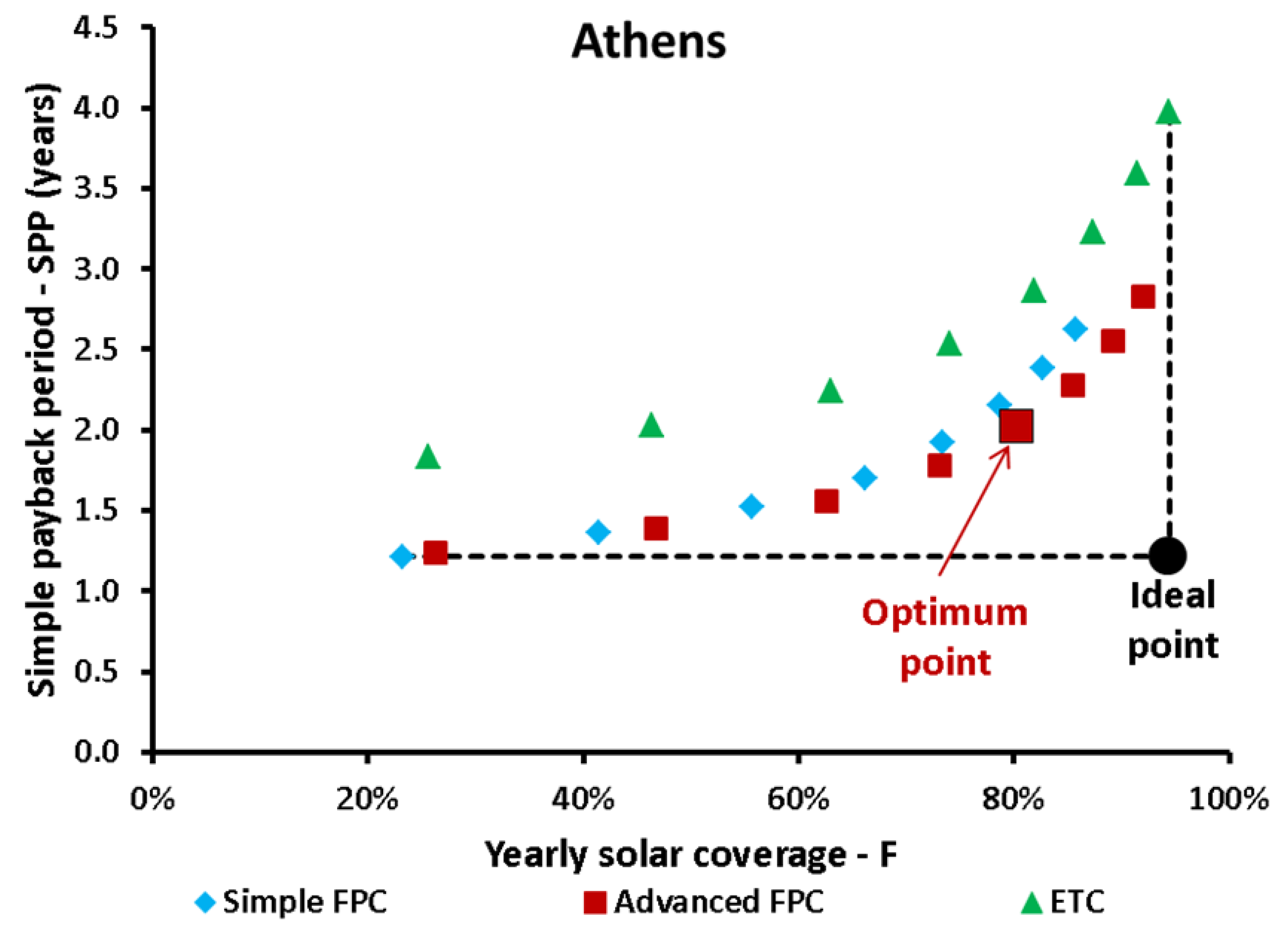
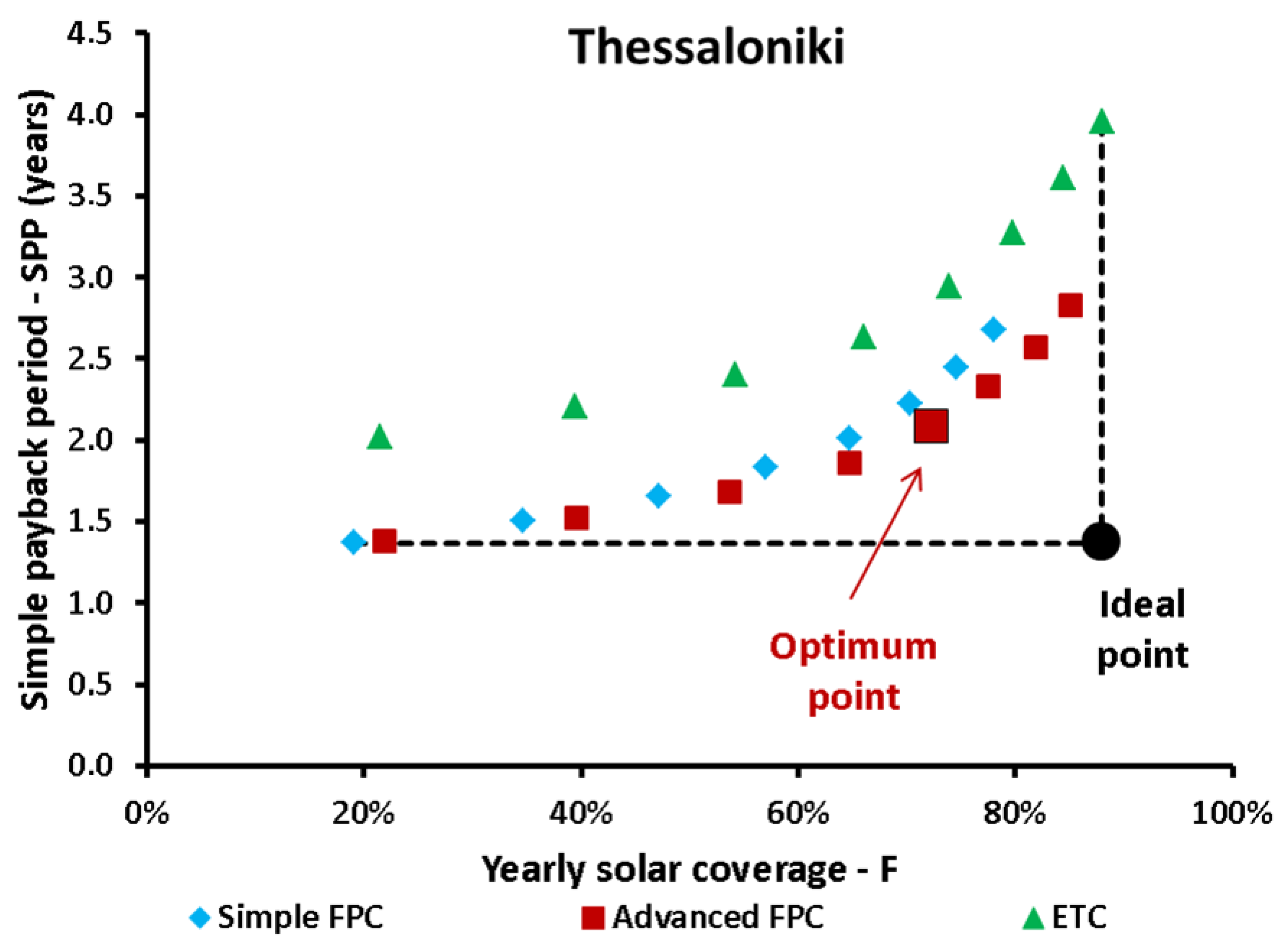
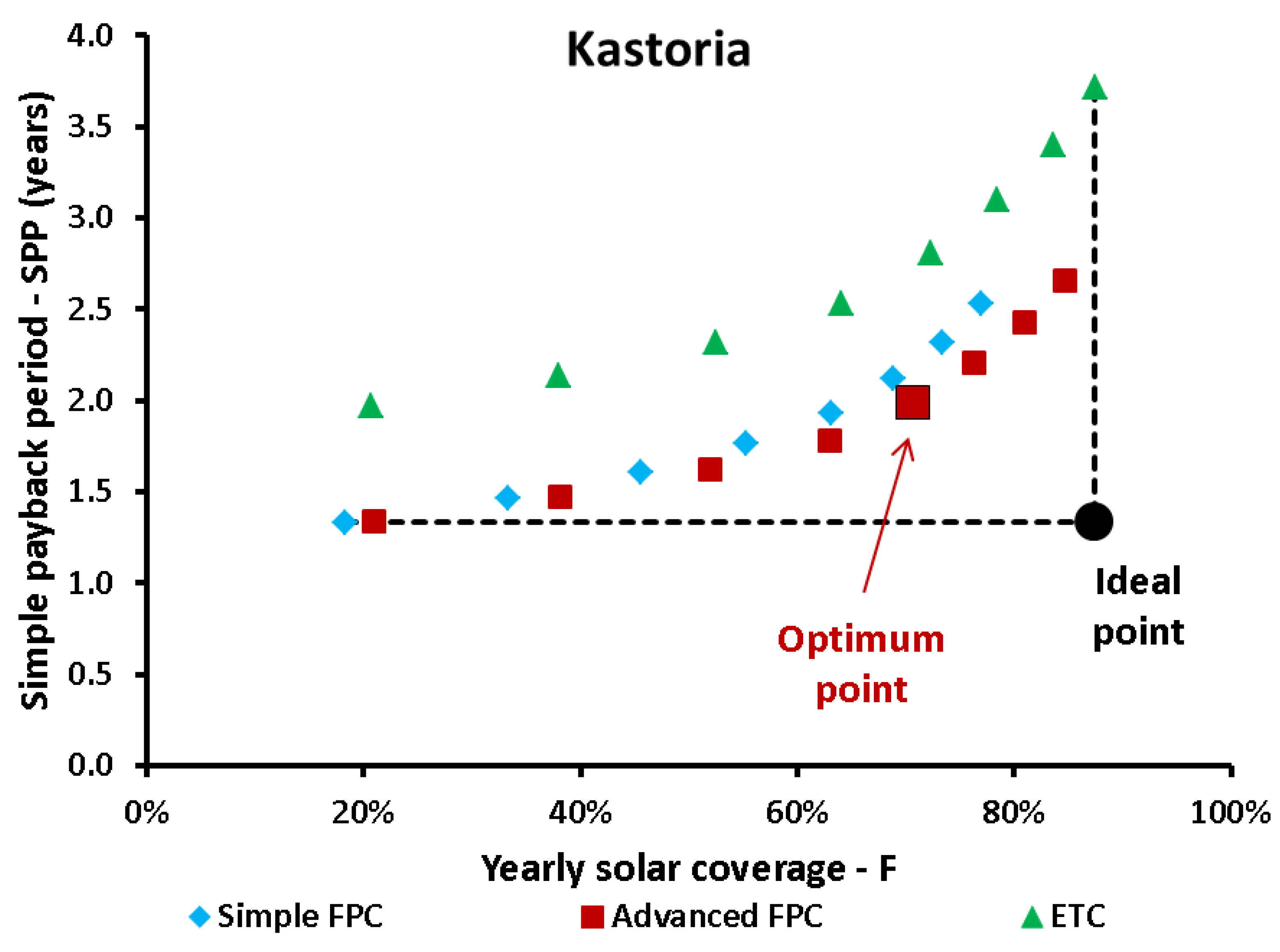
3.4. Multi-Objective Evaluation Procedure

The last step in this study is the multi-objective optimization of the unit by using energy and economic criteria. As it was found in the previous section, the use of the SPP as the sole criterion is not able to lead to energy-efficient designs, and, thus, the combination of the (SPP) and of the (F) is examined through a multi-objective optimization analysis. The objective is to determine the overall optimum choice which combines both low SPP and high F. The described methodology of Section 2.5 is applied, and the goal is to determine the design point with the minimum dimensionless geometric distance from the ideal one, for every city separately. This procedure is a proper one in order to evaluate both criteria in a respective way without taking into account the absolute values of every criterion.
Figure 28, Figure 29, Figure 30 and Figure 31 depict the multi-objective optimization procedures for the cities of Heraklion, Athens, Thessaloniki, and Kastoria, respectively. In every figure, all the design points (combinations of different collectors and collecting areas) are depicted, and the optimum point is the one with the minimum dimensionless distance from the respective ideal one. For all the cities, the optimum collector type is the advanced FPC. This conclusion comes in accordance with the results from the economic optimization according to the LCC minimization criterion. So, there is an accordance in the quality conclusions for the collector type.
The last step is to indicate the global optimum designs according to the multi-objective optimization analysis. Table 8 gives these optimum designs; one for every location. For Athens, Thessaloniki, and Kastoria the optimum collecting area is found at 25 m2, while for Heraklion, the optimum area is 20 m2. The higher solar potential in Heraklion makes possible the proper operation with a bit lower collecting area.
More specifically, for Heraklion, the 20 m2 of collectors have to be placed with a 40° tilt angle which leads to 78.59% solar coverage, 13,731 € LCC, and 1.87 years SPP. For Athens, the 25 m2 of collectors have to be placed with a 45° tilt angle which leads to 80.25% solar coverage, 15,257 € LCC, and 2.03 years SPP. For Thessaloniki, the 25 m2 of collectors have to be placed with a 45° tilt angle which leads to 72.22% solar coverage, 20,257 € LCC, and 2.08 years SPP. For Kastoria, the 25 m2 of collectors have to be placed with a 45° tilt angle which leads to 78.67% solar coverage, 22,193 € LCC, and 1.99 years SPP.
The simple environmental analysis shows the CO2 avoidance due to the use of solar energy for the optimum scenarios of the multi-objective optimization procedure. According to the Greek energy mix, the specific CO2 emissions are 0.487 kg CO2/kWh [36], so this value is used for the calculations in Table 8. It is obvious that there are significant CO2 avoidance values that indicate the high environmental character of the solar thermal systems. More specifically, the yearly CO2 avoidance is 5854 kg CO2/year for Heraklion, 6762 kg CO2/year for Athens, 6573 kg CO2/year for Thessaloniki, and 6896 kg CO2/year for Kastoria.
It is useful to say that the present work indicates relatively low SPP for about two years which are very promising values. These low SPP are lower than other reported in the literature for Greece which was around five years [20,24]. This difference can be explained (i) by the higher electricity price in this work which is representative of the period of the present work and (ii) by the optimization procedure which is done in a proper way by taking into account various parameters.
Another interesting comment is that the optimum collecting areas according to the LCC minimization are greater than the optimum collecting areas obtained by the multi-objective optimization procedure. This is an interesting result that shows that different optimization methods can lead to different results. However, both methodologies indicate that the advanced FPC is the best solar technology. The final selection of the solar field area is depended on the application and the investment type. In cases where the use of solar thermal will be exploited for many years and for the entire time span, then the LCC is the best criterion. On the other hand, when the utilization of the solar system regards a simple retrofitting application or a modification of the energy system which requires a relatively small budget and quick payback period, then the use of the optimum results from the multi-objective optimization work is recommended.
In the future, there is a need for extending this analysis to more cities and for more collector types. Moreover, the results can be compared with results from other models based on dynamic simulations.

4. Conclusions

Solar energy exploitation in the building sector is a vital way to enhance the renewable share in our society. The goal of the present investigation is to examine various solar thermal systems in the Greek climate zones in energy and economic terms. The most essential conclusions are listed in the next bullets:
-
Higher solar field area leads to higher solar coverage and also to a higher optimum tilt angle for all the solar technologies and locations.
-
In the parametric study, it was found that higher efficiency is found with ETC, while the advanced FPC has a bit lower, while the simple FPC has significantly lower performance than the other two choices.
-
The minimization of the LCC indicated that the advanced FPC is the best choice for all the locations. The LCC is 11,088 € for 35 m2 in Heraklion, 12,875 € for 40 m2 in Athens, 16,855 € for 40 m2 in Thessaloniki and 17,692 € for 40 m2 in Kastoria.
-
According to the multi-objective optimization, the advanced FPC is again the optimal choice. For Heraklion, the 20 m2 leads to 78.59% solar coverage and 13,731 € LCC, for Athens, the 25 m2 leads to 80.25% solar coverage and 15,257 € LCC for Thessaloniki, the 25 m2 leads to 72.22% solar coverage and 20,257 € LCC, while for Kastoria, the 25 m2 leads to 78.67% solar coverage and 22,193 € LCC.
-
The SPP period after the multi-objective optimization is found to be around 2 years; a promising value that indicates sustainable and viable assessment.

Author Contributions

E.B.: conceptualization, methodology, investigation, writing—original draft preparation, writing—review and editing; L.P.: methodology, software, validation, formal analysis, investigation, writing—original draft preparation; M.K. (Maria Kekatou): methodology, software, validation, formal analysis, investigation, writing—original draft preparation; M.K. (Michalis Karagiorgas): investigation, writing—original draft preparation, supervision. All authors have read and agreed to the published version of the manuscript.

Funding

Evangelos Bellos would like to thank the Department of Mechanical Engineering Educators of the School of Pedagogical and Technological Education (ASPETE) and ELKE ASPETE for their foundation under the MIS: 5130670.

Institutional Review Board Statement

Not applicable.

Informed Consent Statement

Not applicable.

Data Availability Statement

Data available after request.

Acknowledgments

Evangelos Bellos would like to thank the Department of Mechanical Engineering Educators of the School of Pedagogical and Technological Education (ASPETE) and ELKE ASPETE for their foundation under the MIS: 5130670.

Conflicts of Interest

The authors declare no conflict of interest.

Nomenclature

AcolCollecting area (m2)
a0Zero-order coefficient of the collector efficiency
a1First-order coefficient of the collector efficiency (W/m2K)
a2Second-order coefficient of the collector efficiency (W/m2K2)
cpSpecific heat capacity (J/kgK)
CFgainYearly economic gain—Cash flow (€)
C0Capital cost (€)
DDDimensionless distance in the multi-objective optimization
fMonthly solar coverage
FYearly solar coverage
FRCollector heat removal factor
FR΄System heat removal factor
GTIncident solar irradiation on the tilted surface (W/m2)
HDaily global solar energy on the horizontal surface (kWh/m2)
HdDaily diffuse solar energy on the horizontal surface (kWh/m2)
HTDaily global solar energy on the tilted surface (kWh/m2)
kcolSpecific cost of the solar collectors (€/m2)
kelElectricity cost (€/kWhel)
ktankSpecific cost of the tank (€/m3)
LLoad energy (kWh)
LauxAuxiliary energy consumption (kWh)
Lu,solPart of the load covered by the sun (kWh)
LCCLife cycle cost of the investment (€)
MLifetime of the project (years)
NDays of the month
rDiscount factor
R2Approximation index
RbRatio of the beam irradiation
SPPSimple Payback Period (years)
TamAmbient temperature (°C)
Tam,mMean ambient temperature of the month (°C)
TcoldSupply temperature from the grid (°C)
TfluidOperating fluid temperature (°C)
ThotDesired temperature of the hot water (= 45 °C)
TrefReference temperature (= 100 °C)
Tw,mMean monthly water temperature from the grid (°C)
ULCollector thermal loss coefficient (W/m2K)
VtankStorage tank volume (m3)
VwDaily hot water demand (m3/day)
XParameter for the calculation of the solar coverage
YParameter for the calculation of the solar coverage
Greek Symbols
βCollector tilt angle (°)
βoptOptimum collector tilt angle (°)
δDeclination angle (°)
ΔtTime of the month (s)
ηcolCollector thermal efficiency
ρDensity (kg/m3)
ρgGround reflectance
(τα)Optical efficiency
(τα)nOptical efficiency for normal incident solar irradiation
φLocation latitude (°)
ωsSunset hour angle (°)
ωsSunset hour angle for the tilted surface (°)
Subscripts and Superscripts
maxMaximum value
minMinimum values
Abbreviations
DHWDomestic Hot Water
ETCEvacuated Tube Collectors
FPCFlat Plate Collector

References

  1. United Nations, Department of Economic and Social Affairs. Sustainable Development. 2021. Available online: https://sdgs.un.org/goals (accessed on 15 January 2022).
  2. Hannan, M.; Al-Shetwi, A.Q.; Ker, P.J.; Begum, R.; Mansor, M.; Rahman, S.; Dong, Z.; Tiong, S.; Mahlia, T.I.; Muttaqi, K. Impact of renewable energy utilization and artificial intelligence in achieving sustainable development goals. Energy Rep. 2021, 7, 5359–5373. [Google Scholar] [CrossRef]
  3. Benavente-Peces, C.; Ibadah, N. Buildings Energy Efficiency Analysis and Classification Using Various Machine Learning Technique Classifiers. Energies 2020, 13, 3497. [Google Scholar] [CrossRef]
  4. Liu, J.; Chen, X.; Cao, S.; Yang, H. Overview on hybrid solar photovoltaic-electrical energy storage technologies for power supply to buildings. Energy Convers. Manag. 2019, 187, 103–121. [Google Scholar] [CrossRef]
  5. Shirmohammadi, R.; Aslani, A.; Ghasempour, R.; Romeo, L.M.; Petrakopoulou, F. Techno-economic assessment and optimization of a solar-assisted industrial post-combustion CO2 capture and utilization plant. Energy Rep. 2021, 7, 7390–7404. [Google Scholar] [CrossRef]
  6. Ratajczak, K.; Michalak, K.; Narojczyk, M.; Amanowicz, Ł. Real Domestic Hot Water Consumption in Residential Buildings and Its Impact on Buildings’ Energy Performance—Case Study in Poland. Energies 2021, 14, 5010. [Google Scholar] [CrossRef]
  7. Abd-Ur-Rehman, H.M.; Al-Sulaiman, F.A. Optimum selection of solar water heating (SWH) systems based on their comparative techno-economic feasibility study for the domestic sector of Saudi Arabia. Renew. Sustain. Energy Rev. 2016, 62, 336–349. [Google Scholar] [CrossRef]
  8. Dongellini, M.; Falcioni, S.; Morini, G.L. Dynamic Simulation of Solar Thermal Collectors for Domestic Hot Water Production. Energy Procedia 2015, 82, 630–636. [Google Scholar] [CrossRef] [Green Version]
  9. Knudsen, S. Consumers’ influence on the thermal performance of small SDHW systems—Theoretical investigations. Sol. Energy 2002, 73, 33–42. [Google Scholar] [CrossRef]
  10. Nikolic, D.; Skerlic, J.; Radulovic, J.; Miskovic, A.; Tamasauskas, R.; Sadauskienė, J. Exergy efficiency optimization of photovoltaic and solar collectors’ area in buildings with different heating systems. Renew. Energy 2022, 189, 1063–1073. [Google Scholar] [CrossRef]
  11. Olfian, H.; Ajarostaghi, S.S.M.; Ebrahimnataj, M. Development on evacuated tube solar collectors: A review of the last decade results of using nanofluids. Sol. Energy 2020, 211, 265–282. [Google Scholar] [CrossRef]
  12. Khurana, H.; Majumdar, R.; Saha, S.K. Response Surface Methodology-based prediction model for working fluid temperature during stand-alone operation of vertical cylindrical thermal energy storage tank. Renew. Energy 2022, 188, 619–636. [Google Scholar] [CrossRef]
  13. Gorzin, M.; Hosseini, M.J.; Ranjbar, A.A.; Bahrampoury, R. Investigation of PCM charging for the energy saving of domestic hot water system. Appl. Therm. Eng. 2018, 137, 659–668. [Google Scholar] [CrossRef]
  14. Bilardo, M.; Fraisse, G.; Pailha, M.; Fabrizio, E. Design and experimental analysis of an Integral Collector Storage (ICS) prototype for DHW production. Appl. Energy 2020, 259, 114104. [Google Scholar] [CrossRef]
  15. Martorana, F.; Bonomolo, M.; Leone, G.; Monteleone, F.; Zizzo, G.; Beccali, M. Solar-assisted heat pumps systems for domestic hot water production in small energy communities. Sol. Energy 2021, 217, 113–133. [Google Scholar] [CrossRef]
  16. TOTEE 20701-3/2017; Technical Guidelines; Technical Chamber of Greece: Athens, Greece, 2017.
  17. Bellos, E.; Tzivanidis, C. Solar concentrating systems and applications in Greece—A critical review. J. Clean. Prod. 2020, 272, 122855. [Google Scholar] [CrossRef]
  18. Kaldellis, J.; El-Samani, K.; Koronakis, P. Feasibility analysis of domestic solar water heating systems in Greece. Renew. Energy 2005, 30, 659–682. [Google Scholar] [CrossRef]
  19. Tsilingiridis, G.; Martinopoulos, G. Thirty years of domestic solar hot water systems use in Greece-energy and environmental benefits—Future perspectives. Renew. Energy 2010, 35, 490–497. [Google Scholar] [CrossRef]
  20. Koroneos, C.J.; Nanaki, E.A. Life cycle environmental impact assessment of a solar water heater. J. Clean. Prod. 2012, 37, 154–161. [Google Scholar] [CrossRef]
  21. Martinopoulos, G.; Tsilingiridis, G.; Kyriakis, N. Identification of the environmental impact from the use of different materials in domestic solar hot water systems. Appl. Energy 2013, 102, 545–555. [Google Scholar] [CrossRef]
  22. Balaras, C.A.; Dascalaki, E.; Droutsa, P.; Kontoyiannidis, S. Hellenic renewable energy policies and energy performance of residential buildings using solar collectors for domestic hot water production in Greece. J. Renew. Sustain. Energy 2013, 5, 041813. [Google Scholar] [CrossRef]
  23. Antoniadis, C.N.; Martinopoulos, G. Optimization of a building integrated solar thermal system with seasonal storage using TRNSYS. Renew. Energy 2019, 137, 56–66. [Google Scholar] [CrossRef]
  24. Bellos, E.; Tzivanidis, C. Development of an analytical model for the daily performance of solar thermal systems with experimental validation. Sustain. Energy Technol. Assess. 2018, 28, 22–29. [Google Scholar] [CrossRef]
  25. TOTEE 20701-1/2017; Technical Guidelines; Technical Chamber of Greece: Athens, Greece, 2017.
  26. Beckman, W.A.; Klein, S.A.; Duffie, J.A. Solar Heating Design by the f-Chart Method; Wiley: New York, NY, USA, 1977. [Google Scholar]
  27. Duffie, J.A.; Beckman, W.A. Solar Engineering of Thermal Processes, 4th ed.; Wiley: New York, NY, USA, 2013. [Google Scholar]
  28. Klein, S.; Beckman, W.; Duffie, J. A design procedure for solar heating systems. Sol. Energy 1976, 18, 113–127. [Google Scholar] [CrossRef]
  29. TOTEE 20701-2/2017; Technical Guidelines; Technical Chamber of Greece: Athens, Greece, 2017.
  30. Bellos, E.; Tzivanidis, C.; Antonopoulos, K.A. Exergetic, energetic and financial evaluation of a solar driven absorption cooling system with various collector types. Appl. Therm. Eng. 2016, 102, 749–759. [Google Scholar] [CrossRef]
  31. Bellos, E.; Tzivanidis, C.; Symeou, C.; Antonopoulos, K.A. Energetic, exergetic and financial evaluation of a solar driven absorption chiller—A dynamic approach. Energy Convers. Manag. 2017, 137, 34–48. [Google Scholar] [CrossRef]
  32. Gaglia, A.G.; Tsikaloudaki, A.G.; Laskos, C.M.; Dialynas, E.N.; Argiriou, A.A. The impact of the energy performance regulations’ updated on the construction technology, economics and energy aspects of new residential buildings: The case of Greece. Energy Build. 2017, 155, 225–237. [Google Scholar] [CrossRef]
  33. Liu, B.Y.H.; Jordan, R.C. Daily Insolation on Surfaces Tilted Toward the Equator. ASHRAE J. 1962, 3, 1962. [Google Scholar]
  34. Klein, S. Calculation of monthly average insolation on tilted surfaces. Sol. Energy 1977, 19, 325–329. [Google Scholar] [CrossRef] [Green Version]
  35. Georgousis, N.; Lykas, P.; Bellos, E.; Tzivanidis, C. Multi-objective optimization of a solar-driven polygeneration system based on CO2 working fluid. Energy Convers. Manag. 2021, 252, 115136. [Google Scholar] [CrossRef]
  36. DAPEEP, Residual Energy Mix 2020, June 2021. Available online: https://www.dapeep.gr (accessed on 15 January 2021).
Figure 1. Simplistic presentation of the examined solar thermal system for DHW production.
Applsci 12 04566 g001
Figure 2. Depiction of the collector efficiency and approximation lines (Analysis for Tam = 25 °C and GT = 1000 W/m2).
Applsci 12 04566 g002
Figure 3. The examined cities and the Greek climate zones, Reprinted with permission from ref. [32], Copyright 2015 Elsevier (License Number: 5290151135624).
Applsci 12 04566 g003
Figure 4. The impact of the solar field area and of the tilt angle on the yearly solar coverage for Athens and the simple FPC.
Applsci 12 04566 g004
Figure 5. The impact of the solar field area and of the tilt angle on the yearly solar coverage for Athens and the advanced FPC.
Applsci 12 04566 g005
Figure 6. The impact of the solar field area and of the tilt angle on the yearly solar coverage for Athens and the ETC.
Applsci 12 04566 g006
Figure 7. Optimum tilt angles aiming the solar coverage maximization for Athens.
Applsci 12 04566 g007
Figure 8. Yearly solar coverage with optimum tilt angles for the location of Athens.
Applsci 12 04566 g008
Figure 9. Auxiliary energy consumption with optimum tilt angles for the location of Athens.
Applsci 12 04566 g009
Figure 10. Yearly solar coverage with simple FPC for the examined locations with optimized tilt angle.
Applsci 12 04566 g010
Figure 11. Yearly solar coverage with advanced FPC for the examined locations with optimized tilt angle.
Applsci 12 04566 g011
Figure 12. Yearly solar coverage with ETC for the examined locations with optimized tilt angle.
Applsci 12 04566 g012
Figure 13. Optimum tilt angles for maximizing the solar coverage with simple FPC for the examined locations.
Applsci 12 04566 g013
Figure 14. Optimum tilt angles for maximizing the solar coverage with advanced FPC for the examined locations.
Applsci 12 04566 g014
Figure 15. Optimum tilt angles for maximizing the solar coverage with ETC for the examined locations.
Applsci 12 04566 g015
Figure 16. Auxiliary energy consumption with optimum tilt angles for simple FPC.
Applsci 12 04566 g016
Figure 17. Auxiliary energy consumption with optimum tilt angles for advanced FPC.
Applsci 12 04566 g017
Figure 18. Auxiliary energy consumption with optimum tilt angles for ETC.
Applsci 12 04566 g018
Figure 19. Life cycle cost for different collecting areas and collector types for Heraklion.
Applsci 12 04566 g019
Figure 20. Life cycle cost for different collecting areas and collector types for Athens.
Applsci 12 04566 g020
Figure 21. Life cycle cost for different collecting areas and collector types for Thessaloniki.
Applsci 12 04566 g021
Figure 22. Life cycle cost for different collecting areas and collector types for Kastoria.
Applsci 12 04566 g022
Figure 23. Life cycle cost for different locations with the optimum collector (Advanced FPC).
Applsci 12 04566 g023
Figure 24. Simple payback period for different collecting areas and collector types for Heraklion.
Applsci 12 04566 g024
Figure 25. Simple payback period for different collecting areas and collector types for Athens.
Applsci 12 04566 g025
Figure 26. Simple payback period for different collecting areas and collector types for Thessaloniki.
Applsci 12 04566 g026
Figure 27. Simple payback period for different collecting areas and collector types for Kastoria.
Applsci 12 04566 g027
Figure 28. Multi-objective optimization for the Heraklion city—Zone A.
Applsci 12 04566 g028
Figure 29. Multi-objective optimization for the Athens city—Zone B.
Applsci 12 04566 g029
Figure 30. Multi-objective optimization for the Thessaloniki city—Zone C.
Applsci 12 04566 g030
Figure 31. Multi-objective optimization for the Kastoria city—Zone D.
Applsci 12 04566 g031
Table 1. Thermal efficiency coefficients of the examined solar technologies.
Collector Typea0
(-)
a1
(W/m2K)
a2
(W/m2K2)
Simple FPC0.735.510.006
Advanced FPC0.773.750.015
Collector with evacuated tubes (ETC)0.701.800.020
Table 2. Thermal efficiency parameters of the collectors after the approximation.
Collector TypeFR(τα)
(-)
FRUL
(W/m2K)
R2
(%)
Non-selective simple FPC0.735.8599.93
Selective advanced FPC0.774.5999.34
Collector with evacuated tubes (ETC)0.702.9297.38
Table 3. Data for the daily global solar irradiation on the horizontal surface (H) in [kWh/m2].
CitiesJANFEBMARAPRMAYJUNJULAUGSEPOCTNOVDECYear
Heraklion65.681.6125166.5207.3222.4227.1207.0163.0117.378.661.21722.6
Athens63.377.7118.9152.7190.4207.4214.5198.6156.0111.168.154.41613.1
Thessaloniki52.667.5103.2140.7179.1198.6209.5184.7136.791.456.645.51466.1
Kastoria57.671.3111.2141.1173.6201.8206.3185.5138.597.060.047.71491.6
Table 4. Data for the daily diffuse solar irradiation on the horizontal surface (Hd) in [kWh/m2].
CitiesJANFEBMARAPRMAYJUNJULAUGSEPOCTNOVDECYear
Heraklion27.634.452.666.881.584.384.374.157.242.829.424.8659.8
Athens25.132.050.465.681.885.585.273.755.540.126.321.8643.0
Thessaloniki21.829.247.364.282.086.686.173.153.636.923.118.7622.6
Kastoria22.529.748.164.381.786.686.073.253.737.423.519.1625.8
Table 5. Daily solar energy on the tilt surface (HT) for different tilt angles and locations in [kWh/m2].
β (ο)3035404550β (ο)3035404550
Zone A—Heraklion Zone C—Thessaloniki
JAN3.093.193.273.343.38JAN2.692.802.902.983.04
FEB3.773.853.893.923.93FEB3.283.373.433.473.49
MAR4.604.604.584.544.47MAR3.893.913.913.893.85
APR5.635.545.425.275.10APR4.854.794.714.604.47
MAY6.236.045.835.605.33MAY5.515.375.225.034.83
JUN6.646.406.145.855.54JUN6.095.915.705.475.22
JUL6.676.456.205.925.62JUL6.316.145.935.705.45
AUG6.536.396.216.005.77AUG5.985.875.745.575.38
SEP5.995.965.905.815.68SEP5.155.155.125.074.98
OCT4.804.874.924.944.92OCT3.873.954.014.044.05
NOV3.803.924.024.094.14NOV2.893.003.093.163.22
DEC3.023.133.233.313.36DEC2.442.562.662.742.80
β (ο)3035404550β (ο)3035404550
Zone B—Athens Zone D—Kastoria
JAN3.173.293.403.483.54JAN2.993.133.243.333.40
FEB3.733.823.883.933.94FEB3.503.593.663.713.73
MAR4.474.494.484.454.40MAR4.234.264.264.244.20
APR5.235.165.064.944.79APR4.874.814.724.624.49
MAY5.805.655.475.275.05MAY5.345.215.064.884.69
JUN6.296.095.865.615.34JUN6.186.005.795.555.30
JUL6.406.215.995.755.48JUL6.226.045.845.625.37
AUG6.376.256.095.915.69AUG6.005.905.765.605.41
SEP5.855.845.805.735.62SEP5.235.235.205.145.06
OCT4.694.794.854.894.89OCT4.144.234.294.334.34
NOV3.413.533.643.723.77NOV3.093.213.323.403.46
DEC2.832.953.063.153.22DEC2.582.702.812.902.97
Table 6. Mean monthly air temperature (Tam,m) and mean water temperature from the grid (Tw,m) expressed in [°C].
HeraklionAthensThessalonikiKastoria
Tam,mTw,mTam,mTw,mTam,mTw,mTam,mTw,m
JAN12.114.78.711.35.38.22.24.2
FEB12.214.29.310.96.87.93.45.0
MAR13.514.811.211.89.89.26.97.5
APR16.517.215.414.314.312.811.511.5
MAY20.320.620.717.719.716.816.415.7
JUN24.424.525.721.624.520.221.419.8
JUL26.227.328.124.726.821.524.022.2
AUG26.128.227.525.726.222.823.222.7
SEP23.627.223.424.221.922.118.920.2
OCT20.124.718.221.116.319.413.415.9
NOV16.720.913.816.911.115.77.210.8
DEC13.717.210.313.56.911.03.06.6
Table 7. Summary of the optimum designs according to the maximization of the life cycle cost index.
Zone A—Heraklion
Collector typeAcol (m2)βopt (°)FLCC (€)SPP (years)
Simple FPC405089.37%12,3832.85
Advanced FPC355092.55%11,0882.78
ETC305091.35%13,4803.49
Zone B—Athens
Collector typeAcol(m2)βopt(°)FLCC (€)SPP (years)
Simple FPC404585.77%14,7372.63
Advanced FPC405092.05%12,8752.83
ETC355091.50%15,5183.59
Zone C—Thessaloniki
Collector typeAcol(m2)βopt(°)FLCC (€)SPP (years)
Simple FPC405077.97%19,4052.68
Advanced FPC405085.09%16,8552.83
ETC405087.98%19,3293.95
Zone D—Kastoria
Collector typeAcol(m2)βopt(°)FLCC (€)SPP (years)
Simple FPC405077.01%20,7842.53
Advanced FPC405084.61%17,6922.65
ETC405087.41%20,1103.71
Table 8. Final summary of the optimum designs according to the multi-objective optimization.
CityCollector TypeAcol
(m2)
βopt
(°)
F
(%)
LCC
(€)
SPP
(years)
CO2 Avoidance (kg/year)
HeraklionAdvanced FPC204078.5913,7311.875854
AthensAdvanced FPC254580.2515,2572.036762
ThessalonikiAdvanced FPC254572.2220,2572.086573
KastoriaAdvanced FPC254570.6722,1931.996896
Publisher’s Note: MDPI stays neutral with regard to jurisdictional claims in published maps and institutional affiliations.

