Article

Influence of Initial Conditions on Wind Characteristics at a Bridge Middle Span in a U-Shaped Valley by CFD and AHP

1
School of Highway, Chang’an University, Xi’an 710064, China
2
Wind Tunnel Laboratory, Chang’an University, Xi’an 710064, China
*
Author to whom correspondence should be addressed.
Submission received: 5 April 2022 / Revised: 1 May 2022 / Accepted: 1 May 2022 / Published: 6 May 2022
(This article belongs to the Topic Multi-Criteria Decision Making)

Abstract

:
The wind parameter distribution law at a bridge midspan in a U-shaped valley has important influence on the wind strength of this bridges. In this paper, the wind characteristics were researched by computational fluid dynamics (CFD). The surface roughness, the inlet wind speed, the wind speed profile, and the oncoming wind direction were selected as the initial conditions; the wind speed, the wind attack angle, and the wind azimuth angle were set as wind parameters; and the effect of the four initial conditions on the wind parameters was comprehensively analyzed. An innovative quantification model used to connect the coefficient of sensitivity factors with scale values was established, and the influence of initial conditions on wind parameters was studied by analytic hierarchy process (AHP) for the first time. The results show that the spatial distribution of wind characteristics in a U-shaped valley is complex and obviously affected by the initial conditions. The established quantification model has certain practicability. The AHP evaluation results showed that the influence of the oncoming wind direction on wind parameters was the most obvious. The influence degree of oncoming wind direction and wind speed profile on wind speed was just as important, accounting for 77.4%. The sensitivity of wind attack angle to oncoming wind direction was 60.8%, which was much higher than the surface roughness, inlet wind speed, and wind speed profile. The influence degree of oncoming wind direction on wind azimuth angle was the sum of the other three initial conditions.

1. Introduction

At present, the study of wind parameters in valley areas is one of the hot spots of wind engineering research. In mountainous valley areas, the temporal and spatial variations of wind parameters are complex, and there is no uniform law. The influence of wind on the design, construction, and service of long-span bridges cannot be ignored, and are even among the controlling factors.
Research on the wind characteristics of a valley is mainly based on field measurements [1,2], wind tunnel tests [3], and numerical simulations. Although field measurement can directly obtain the wind parameter data at the measured position, it is time-consuming, labor-intensive, and requires huge investment, and the obtained wind parameters are limited in quantity, time, and space. On the other hand, the wind tunnel test is widely used, but there are some problems with the accuracy of feature flow simulation and scale model production. Finally, with the development of computer technology, computational fluid dynamics (CFD), the convenient operation and lower cost, numerical simulation is more widely used, and the reliability has been verified [4,5].
In terms of CFD simulation, Chung and Bienkiewicz [6] discussed the application of three turbulence models—modified k–ε model, standard k–ω model, and the standard—and it was found that was more consistent with the experimental data than the other two models. Braun and Awruch [7] used the pseudo-compressibility approach, large eddy simulation (LES), an arbitrary Lagrangean–Eulerian (ALE) formulation, and an explicit two-step Taylor–Galerkin method to simulate two-dimensional viscous turbulence. Li et al. [8] combined the weather model, RAMS, and the computational fluid dynamics model, FLUENT, into a one-way offline nested modeling system. Yan et al. [9] proposed a phase delay spectrum model to represent the spatial coherence of random wind fields. Wang et al. [10] used numerical simulation to study the neutral stratified turbulent boundary layer on a two-dimensional hill. Ren et al. [11] proposed a method of fine-tuning observations based on spatial correlation, which could consider the impact of complex terrain. Liu et al. [12] proposed an improved scheme involving only a basic random variable dimensionality reduction mode and non-uniform wavenumber interval. Lu et al. [13] used the RANS/LES hybrid model to numerically analyze the external flow field of the terrain, studied the wind speed amplification factor and the change law of wind parameters along the height, and discussed the canyon effect and thinning effect of the wind field. Based on the twisted wind profile conditions of the quasi-steady state theory, Li et al. [14] evaluated the influence of wind field characteristics on the buffeting response of a variable cross section bridge tower, where the bridge is located in a trumpet-shaped mountain pass. Wang et al. [15] used the CFD-based numerical simulation method to establish a numerical model of the canyon bridge-tunnel junction. Huang et al. [16] analyzed the wind directions’ effect on wind characteristics over complex terrain by CFD. Song et al. [17] also discussed the influence of wind direction on wind speed along the bridge axis.
In summary, scholars have undertaken many numerical studies on wind parameters at mountainous bridge sites, but only one or two of the factors such as oncoming wind direction, inlet wind speed, wind speed profile, or surface roughness were considered. However, the simultaneous influence of these initial conditions on wind parameters has not considered, and their influence degree of initial conditions remain unexplained.
On the other hand, the analytic hierarchy process (AHP) is a combination of qualitative and quantitative decision-making methods that are widely used in safety production technology evaluation, reliability evaluation, water quality index research, and other areas. It can quantitatively analyze the importance of multiple factors affecting an object, which is conducive to grasping key points of the problem. Therefore, the AHP was introduced as follows. Bakioglu and Atahan [18] used the interval value Pythagorean Fuzzy analytic hierarchy process to evaluate the weight coefficients of factors that affect the adoption of autonomous vehicles. Chen and Dai [19] proposed the analytic hierarchy process (AHP) of group decision-making based on the confidence index to construct a weighted cloud model. Ma et al. [20] used the analytic hierarchy process to evaluate, built a judgment matrix through expert scoring analysis, and then calculated a new weight for each DRASTIC parameter, which can reduce subjectivity to a certain extent, and the weight value tends to stabilize. Merhi et al. [21] used the AHP to study the critical success factors of data intelligence implementation in the public sector. Radhika et al. [22] conducted budget optimization of dynamic virtual machine provision by AHP whereas, at present, reports on the application of the analytic hierarchy process in bridge wind engineering are few. The reason may be the lack of a reliable mathematical model linking AHP and bridge wind engineering.
This paper used a U-shaped valley as the research object. The aim of this paper was to analyze the influence of the initial conditions on wind characteristics at a bridge site in a U-shaped valley. Through the numerical simulation method, the four initial conditions (surface roughness (five working conditions), inlet wind speed (five working conditions), wind speed profile (five working conditions), and oncoming wind direction (five working conditions, but one was the same as before) were considered in turn, and 19 working conditions were designed to obtain the distribution law of wind speed, wind attack angle, and wind azimuth angle at the middle of the bridge span. Then, a mathematical model of wind parameter factors and scale value was established, and the numerical calculation results and analytic hierarchy process were connected by the model. On this basis, the sensitivity of wind parameters to the four initial conditions was analyzed. This research can provide a reference for the simulation of wind fields and promote an understanding of the influence of the initial conditions on the wind parameter distribution in valley areas.

2. Numerical Calculation Model

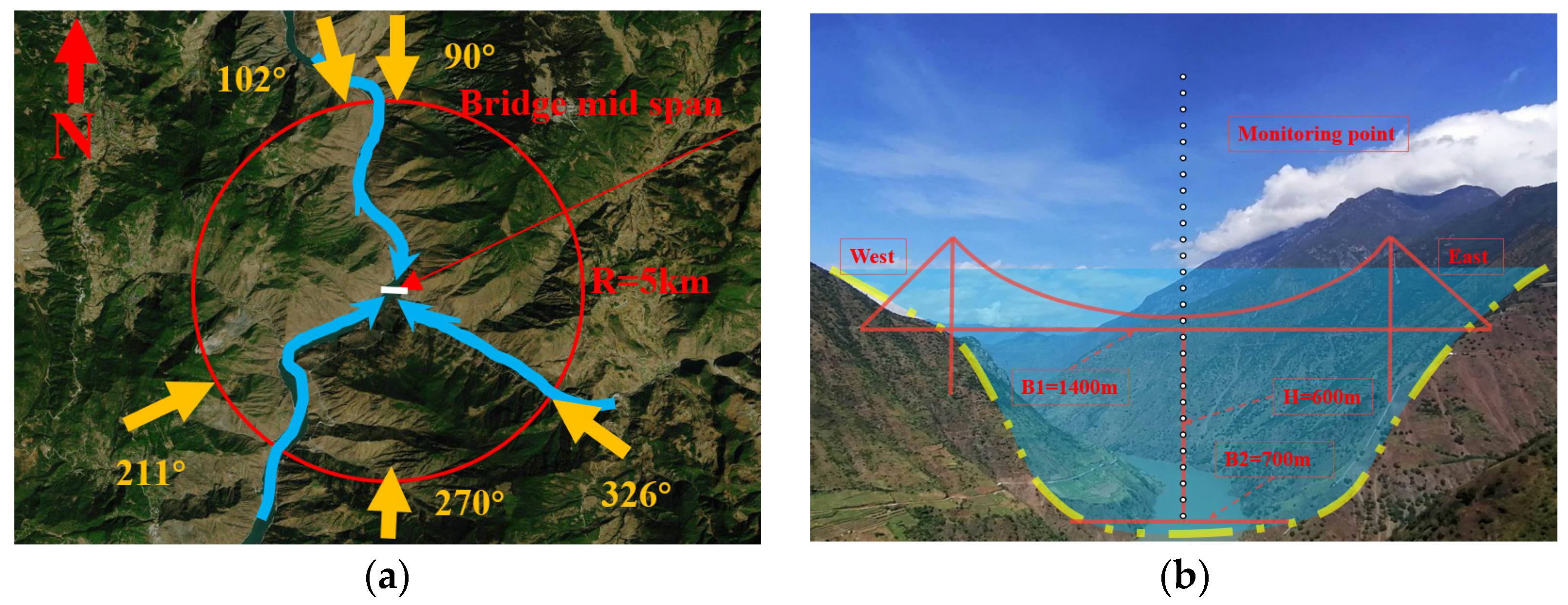
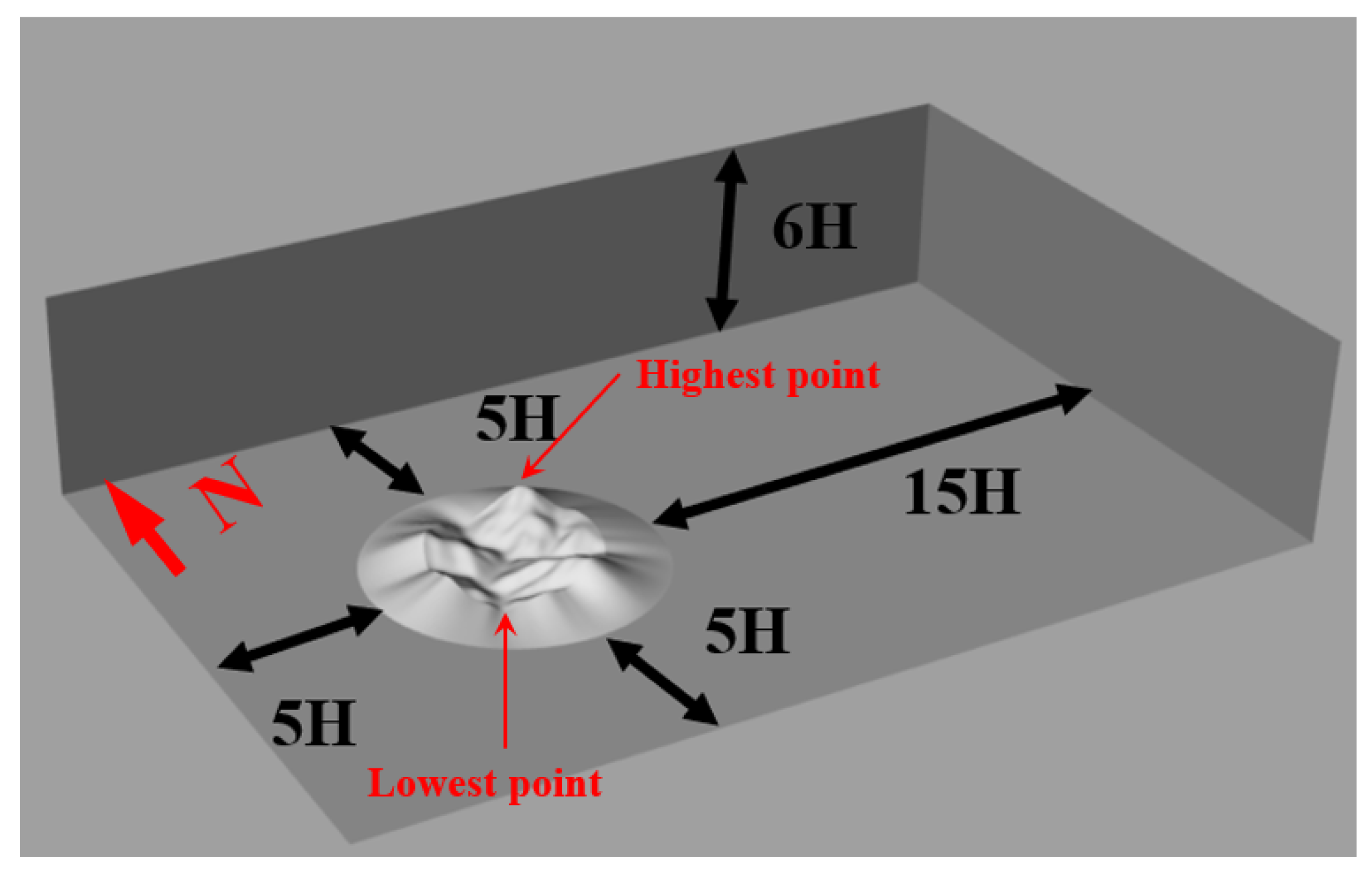
2.1. Terrain and Calculation Domain
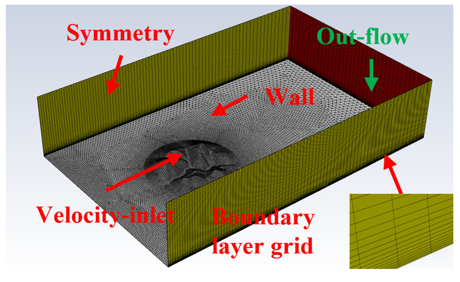
The U-shaped valley in this study is located in the Jinsha River section of Lijiang City, Yunnan Province, China. There are high mountains and deep valleys in this area, where a long-span suspension bridge will be built, and the bridge span is about 1400 m [23]. The bridge will span the river surface, and the height difference between the bridge deck and the river surface is about 600 m, as shown in Figure 1.
With the intersection point of the U-shaped valley as the center, the contour was created from the terrain with a radius of 5 km to generate the terrain surface of the valley. Based on a suggestion by Blocken [24], the lowest point of the calculation domain was located downstream of the river in the southwest direction, which was set as the height base point, 0 m. The highest point in the calculation domain was located at the southeast mountain peak, which represents the maximum elevation difference in the valley, denoted as H, 2075 m, as shown in Figure 2. In order to reduce the influence of the “artificial cliff” [25], a slope transition section with a maximum gradient of 30° was set, with a horizontal length of 3600 m, forming the calculation domain of the cylindrical internal cylinder. The size of the rectangular calculation domain was 18.975 km (width) × 58.7 km (length) × 12.45 km (height).

2.2. FLUENT Setting

FLUENT software, a fully implicit separation solver suitable for incompressible and low-velocity flows, was used for numerical simulation and an unsteady shear stress transport k–ω turbulence model [26,27], suitable for flow around bluff bodies, was selected. The SIMPLE algorithm calculates pressure–velocity coupling. The momentum equation, turbulent kinetic energy, and transport dissipation rate equations adopted the second-order upwind discrete scheme, and the residual convergence accuracy was taken as 1.0 × 10⁻⁶.
Considering the complex variation of wind characteristics in a mountainous valley, first, the steady model was used to solve and the flow field was initialized. After the calculation was stable, the transient model was used for solving [28]. According to the requirements of Courant–Friedrichs–Levy (CFL) parameters in FLUENT [29], the transient solution time should ensure that each iteration can be within a grid range and eliminate cross-grid errors, as shown in Equation (1). The CFL is computed by the solver and used to ensure the success of the simulation. The time step was set to 0.8 s, and the total time was 6000 s. After trial calculations, wind speed and air volume converged when the working condition reached 4500 s, so these values at the monitoring point were obtained by averaging the wind speed time series of the last 1000 s.
C F L = U Δ t Δ L < 1
where U is the inlet wind speed (m/s); Δ t is the time step (s); and Δ L is the minimum grid length (m).

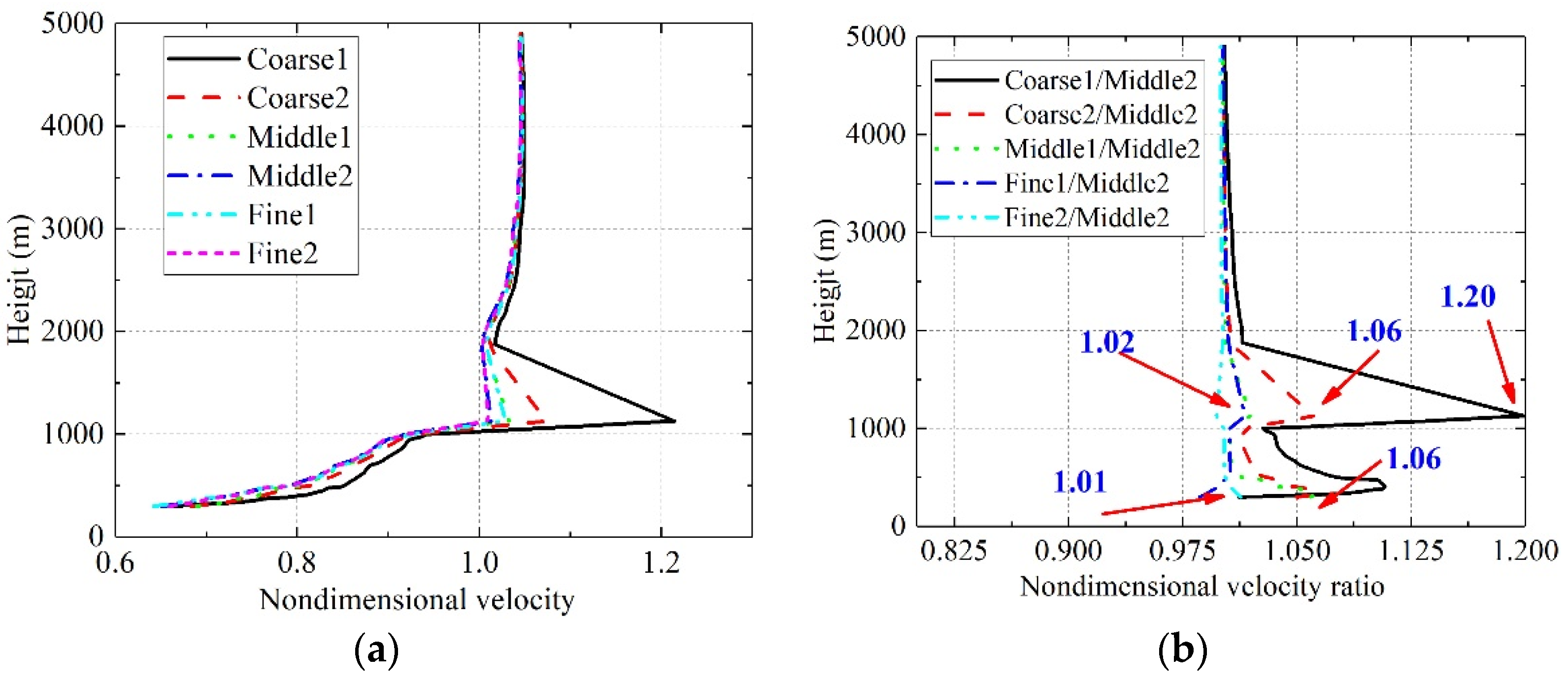
2.3. Mesh Division and Independence Validation

In order to improve the reliability of numerical simulation, grid independence validation research was carried out. The grid was generated by Gambit software, and was divided into six groups, as shown in Table 1, which increased from 2.9 million to 16.13 million in turn. Preliminarily judging by the nondimensional velocity profile trend at the monitoring point (Figure 1b), the nondimensional velocity profile of the Middle2 precision grid condition was seen to be in good agreement with that of the higher precision grid condition, as shown in Figure 3a. At the same time, the nondimensional velocity ratio was defined by the velocity of the Middle2, dividing the other cases at the same height. Due to the maximum of the nondimensional velocity ratio, ranged from 1.01 to 1.20, and 1.01–1.02 represents the relationship between the Middle2 and Fine1, Fine2. Furthermore, it can also be seen from Figure 3b that the accuracy of the Middle2 precision grid calculation was higher. Considering the numerical simulation accuracy and calculation cost, the Middle2 precision grid was finally selected as the calculation grid, and the number of grids was 11.5 × 10⁷. Triangular mesh was used on the ground, and triangular prism mesh was used as a whole. Taking into account the subsequent roughness, based on Blocken’s suggestion [24], the first mesh boundary layer was 5 m and the growth rate was 1.15, for a total of 10 layers. The last layer of the mesh was 17.6 m and the total height of the boundary layer was 101.5 m, as shown in Figure 4.

3. Analytic Hierarchy Process and Initial Conditions

3.1. Analytic Hierarchy Process

The analytic hierarchy process (AHP) is a quantification method for processing qualitative problems that can be used to analyze the weight index of complex problems. The basic steps are as follows:
(1) Analyze the primary and secondary relations among various factors of the system and construct a hierarchical structure, which is generally divided into the highest level target layer, the middle level criterion layer, and the lowest level scheme layer. The number of elements in the criterion and scheme layers should not exceed nine.
(2) For each element at the same level, make pairwise comparisons for the importance of a certain criterion at the previous criterion level, and construct judgment matrix A = ( a i j ) n × n for pairwise comparisons, as shown in Table 2.
(3) Calculate the weight vector w i and consistency index ( C I ) of each element of a certain criterion according to the judgment matrix, and check the consistency ratio ( C R ). C R < 0.1 is required, and the next step can be performed only if the consistency check is satisfied; otherwise go back to step 2 to modify the judgment matrix.
Weight vector w i calculation methods include geometric average (square root), arithmetic average (summation), eigenvector, and least square methods. Since the value of each column in the judgment matrix approximately reflects the weight, the arithmetic average of all column vectors can be used to calculate the weight vector. Therefore, this paper adopted the arithmetic average method. The calculation steps are as follows. Calculate a i j / k = 1 n a k j and normalize the judgment matrix elements by column, and then add and divide the normalized columns to obtain the weight vector, as shown in Equation (2):
w i = 1 n j = 1 n a i j k = 1 n a k j
C I = λ max n 1
where λ max is the maximum eigenvalue of the judgment matrix A = ( a i j ) n × n , and n is the order of the judgment matrix.
C R = C I R I
where R I is the random consistency index, as shown in Table 3.
(4) Calculate the score according to the weight matrix, sort the weight of the factors, and provide evaluation suggestions.

3.2. Initial Conditions

According to the FLUENT calculation results, the wind speed component in three directions of the monitoring point position could be obtained: downwind speed u , crosswind speed v , and vertical wind speed w , and the directions are consistent with the Cartesian coordinate system in the calculation domain. Wind attack angle α and wind azimuth angle β can be calculated according to Equations (5) and (6). Second, nondimensional wind speed factor u ¯ , wind attack angle factor α ¯ , and wind azimuth angle factor β ¯ are defined and calculated by Equations (7)–(9), respectively.
a = a c t a n w u 2 + v 2
β = a c t a n v u
u ¯ = u U r e f
α ¯ = α α r e f
β ¯ = β β r e f
where U r e f is wind speed at a certain height; α r e f is reference wind attack angle at a certain height; and β r e f is reference wind azimuth angle at a certain height.

4. Results and Discussion

4.1. Influence of Initial Conditions on Wind Parameter

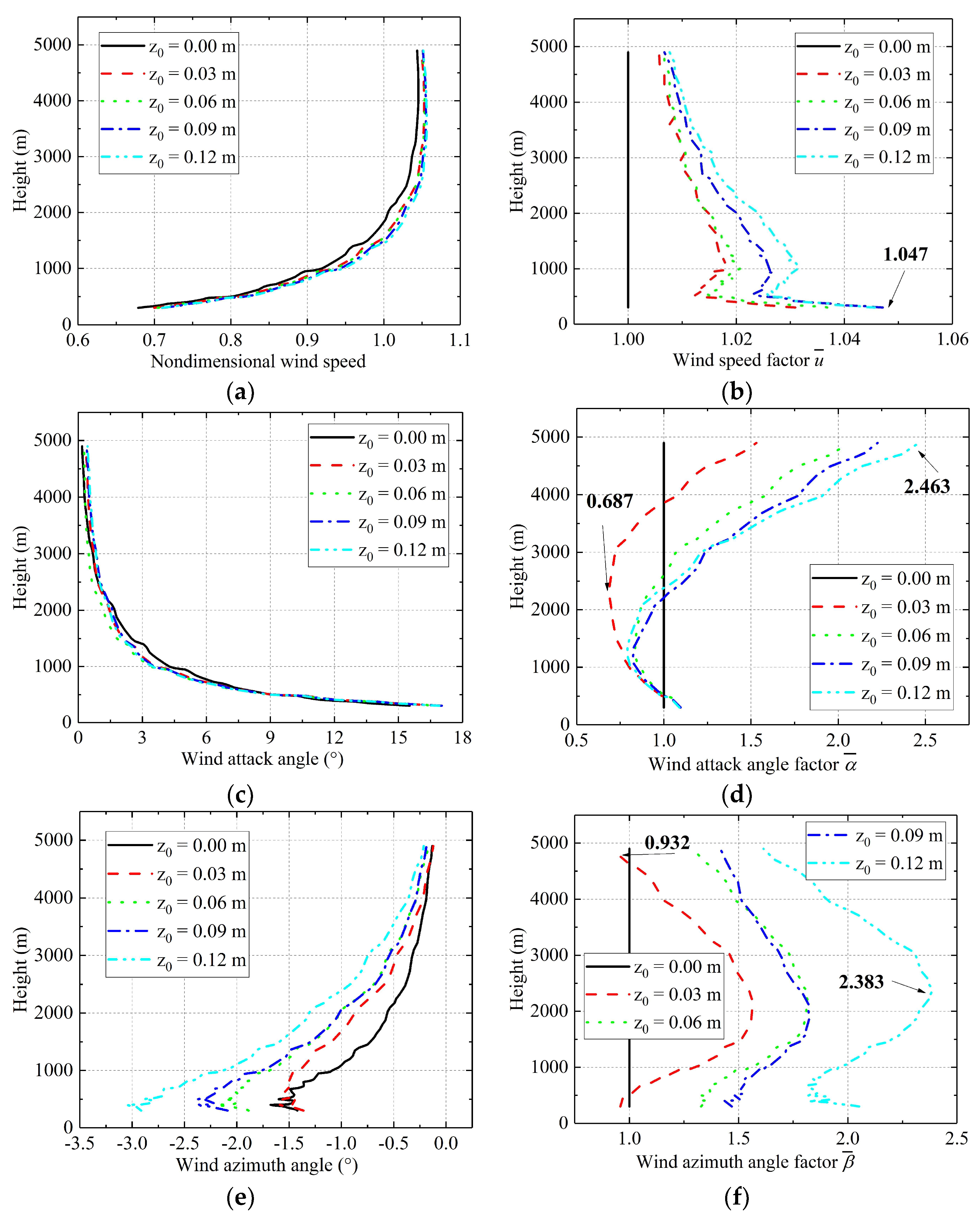
4.1.1. Surface Roughness

Under the influence of surface roughness, the wind speed near the ground will be reduced to 0. The simulation of surface roughness was summarized by Pattanapol et al. [30], which was divided into two methods: wall function and adding original resistance term. The wind speed calculation results of the two methods were quite different at low altitude. Pattanapol et al. [30], Blocken et al. [31], and others used the wall function to simulate the roughness of complex terrain. Therefore, in this section, the surface roughness was simulated by setting the wall function. The setting of roughness value z 0 , referred to as Blocken’s recommendations [24,32,33], as shown in Equation (10):
z 0 = K S C S 9.793
where z 0 is the surface roughness (m); K S is roughness height (m), which is related to the grid size and should not be less than two times the vertical distance h p from the centroid of the first layer of grid to the bottom; and C S is the roughness coefficient, which was 0.5 by default, indicating uniform roughness, and for uneven roughness, the value was 0.5–1.
As for Equation (10), it is suitable for use for CFD based on ANSYS. As the C S ranged from 0.5–1, the required cell height was limited to some extent by the maximum of C S , especially for the lowest boundary layer cell [32].
Therefore, roughness z 0 was successively set as 0, 0.03, 0.06, 0.09, and 0.12 m, meeting the requirements of Equation (10). The inlet wind speed was taken as 27.1 m/s, according to the 100-year return period wind speed [34] of Lijiang meteorological station, which is the nearest station to the bridge site, so the wind speed at gradient wind height was 27.1 m/s. Taking 102° oncoming flow as an example, the influence of surface roughness on wind parameters is shown in Figure 5. Then taking the condition with the surface roughness of 0 m as the reference condition, and according to Equations (7)–(9), the nondimensional factors are shown in Figure 5b,d,f.
It can be seen from Figure 5 that, compared with the working condition without setting surface roughness, the influence of surface roughness on wind parameters cannot be ignored. The higher the surface roughness, the more obvious the influence on wind speed, wind attack angle, and wind azimuth angle. The surface roughness has a greater influence on the wind attack angle and wind azimuth angle than on wind speed profile. Specifically, the higher the roughness, the more obvious the influence on low-level wind speed below 1000 m. The maximum wind speed factor was about 1.05. The wind speed factor decreased gradually with increased height, and wind speed above 1000 m increased by about 1%. The influence of surface roughness on the wind attack angle varied with height and surface roughness. The higher the surface roughness, the higher the change in wind attack angle at a 5000 m altitude, with a maximum of about 2.5 times. The wind attack angle factor first decreased and then increased with height. Second, the higher the surface roughness, the larger the wind azimuth angle, and the influence on the wind azimuth angle at low altitude was more obvious. From the wind azimuth angle factor, the influence of roughness increased and then decreased, and the maximum amount was about 2.4 times. The wind azimuth angle factor first increased and then decreased with height.
According to the survey of the landform of the bridge site, there are weeds on both sides of the river, and some low trees are scattered on the ridges on both sides. The roughness length in the study was set as 0.12 m.

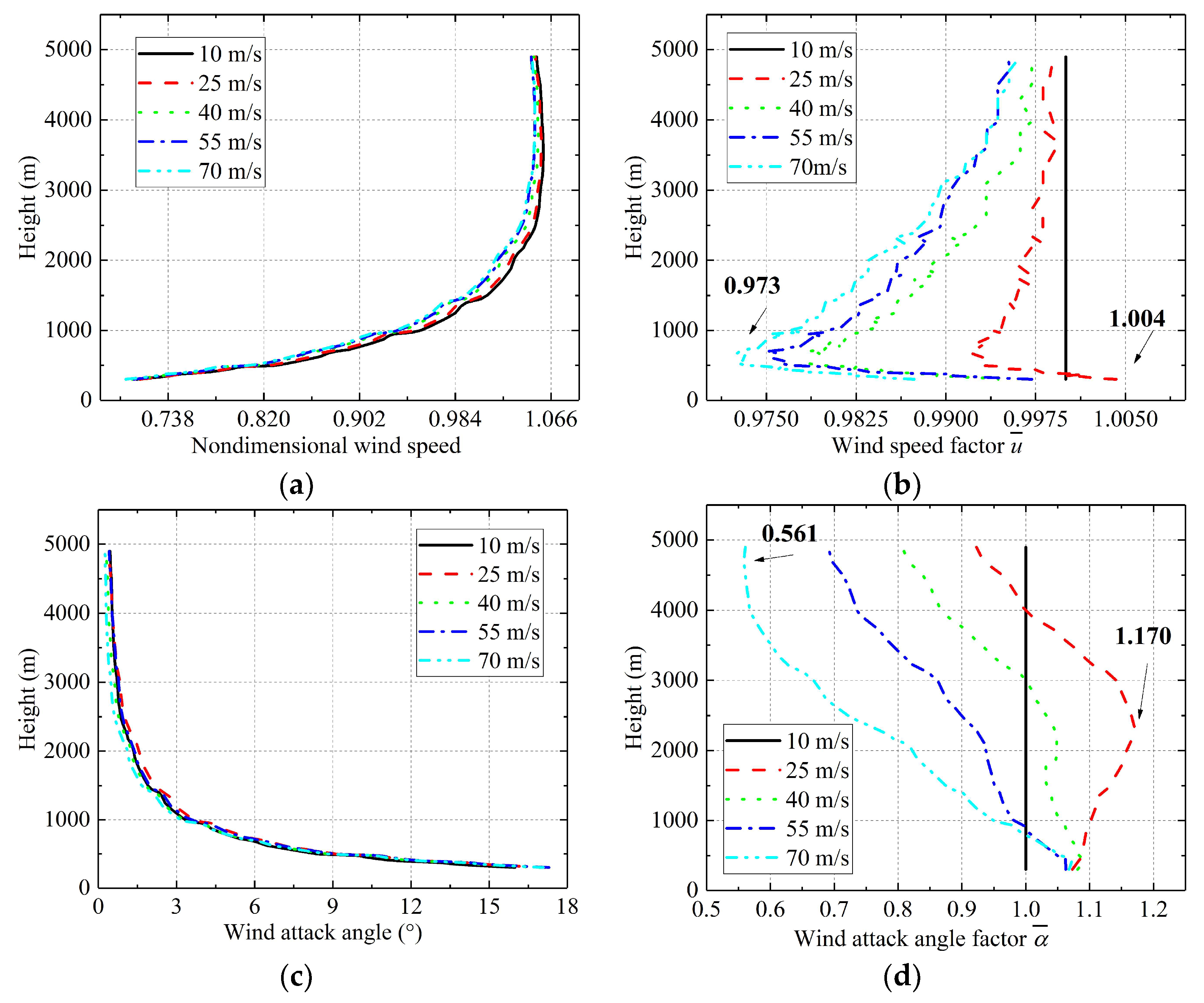
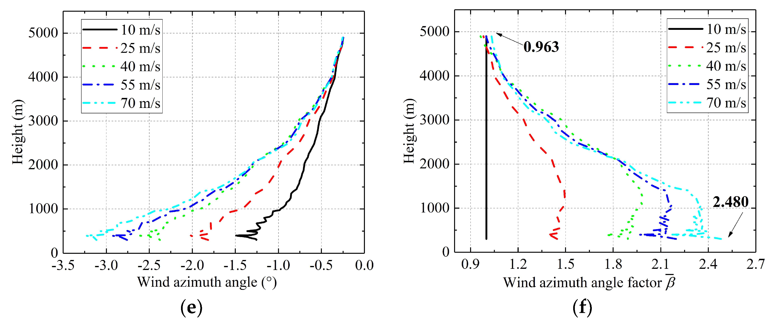
4.1.2. Inlet Wind Speed

Based on the previous section, in order to analyze the influence of inlet wind speed on wind parameters, the uniform oncoming flow was also set; the wind speed was 10–70 m/s, the interval was 15 m/s, and a roughness length of 0.12 m was set. Similarly, taking 102° oncoming flow as an example, the results are shown in Figure 6. Then, taking the condition with the inlet wind speed of 10 m as the reference condition, and according to Equations (7)–(9), the nondimensional factors are shown in Figure 5b,d,f.
As can be seen from Figure 6, taking the oncoming flow of 10 m/s as a reference, the influence of inlet wind speed on the wind speed profile was not obvious, the wind speed factor fluctuated within 3%, and it tended to increase then decrease with height. However, the influence of inlet wind speed on wind attack angle and wind azimuth angle could not be ignored. Specifically, the higher the inlet wind speed, the smaller the wind attack angle in a high position. For example, at a height of 4000 m, the wind attack angle factor under 10 m/s was about twice that under 70 m/s; at the same time, the higher the inlet wind speed, the higher the low-level wind azimuth angle. For example, at 500 m height, the wind azimuth angle under 70 m/s was about 3.0°, and the wind azimuth angle factor was about 2.5 times that under 10 m/s.

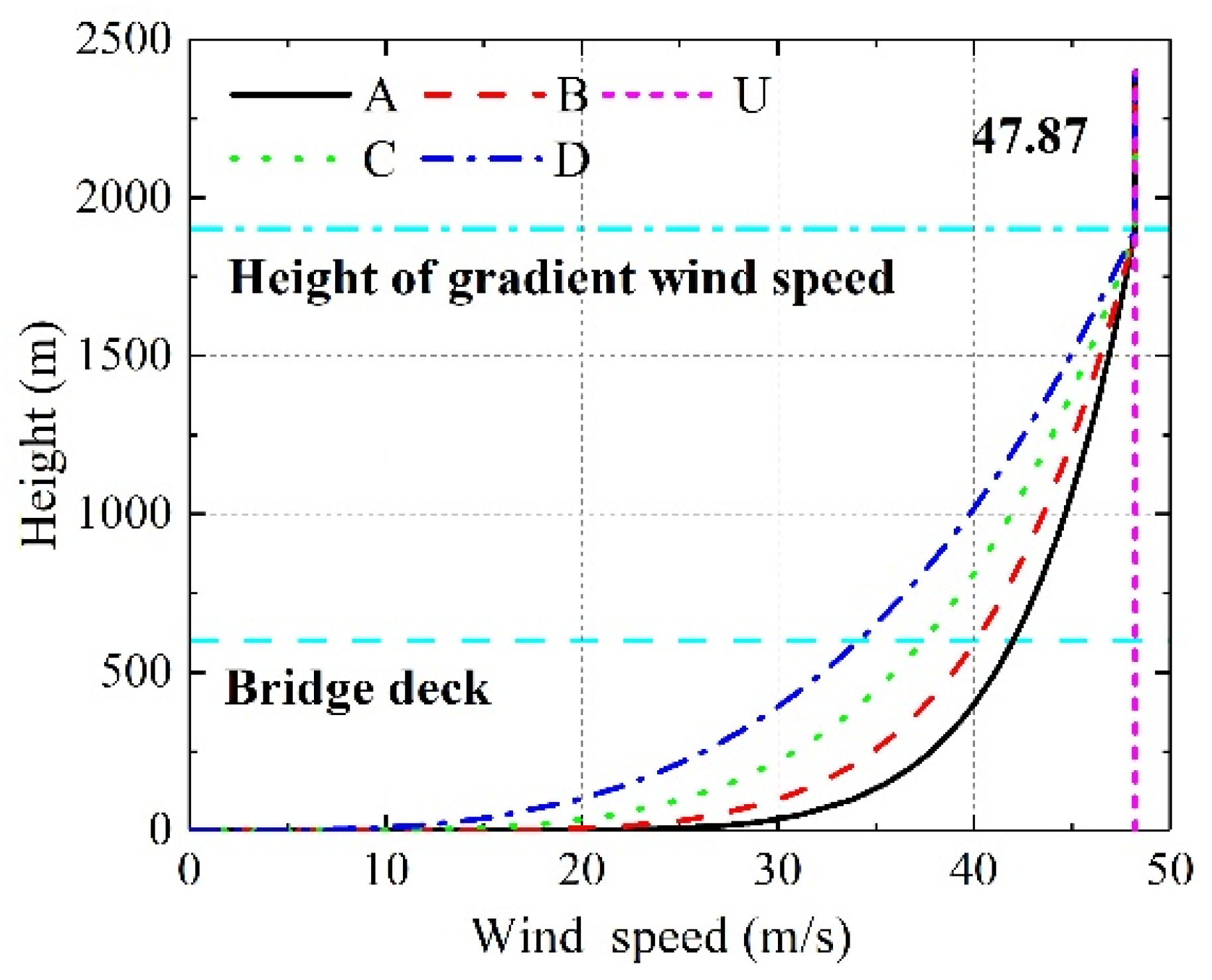
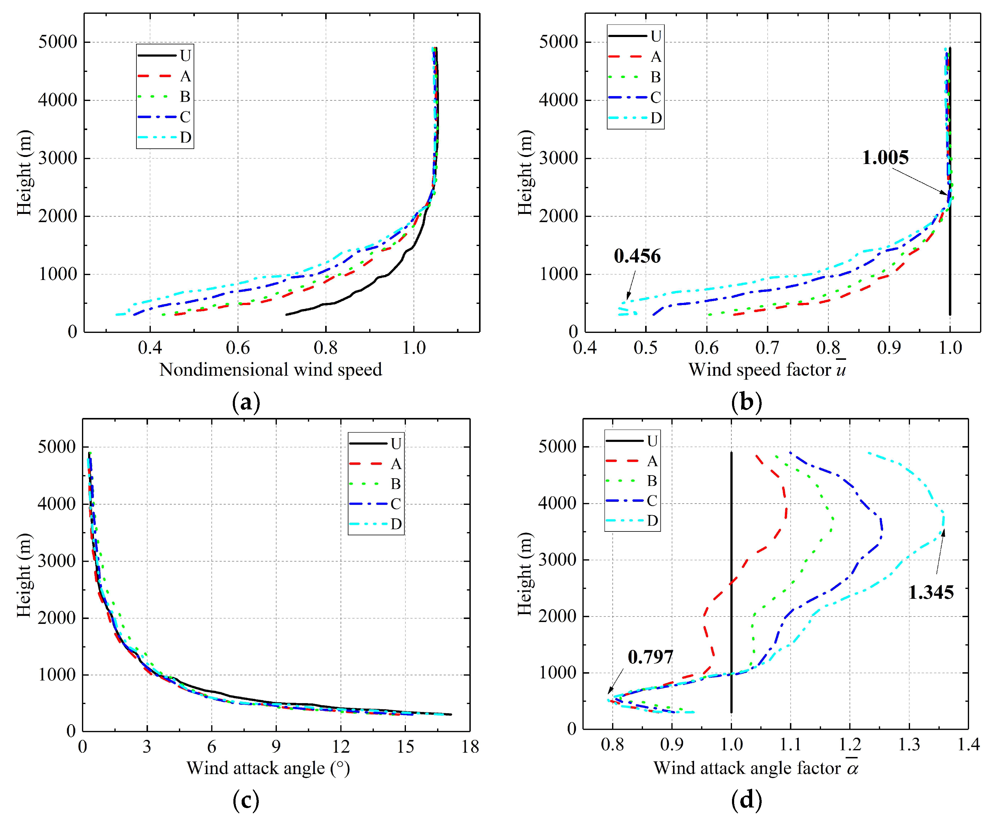
4.1.3. Wind Speed Profile

Based on the previous section, surface roughness height of 0.12 m was set. Similarly, taking 102° oncoming flow as an example, the wind speed profile adopted followed the recommendations by Zhang et al. [35]. As above-mentioned, we used the outlet of the downstream river in the southwest as the elevation base point, set as 0 m, and the height difference between it and the peak in the southeast, 2075 m. The average height of the surrounding mountains was about 1550 m, and the gradient wind height was about 350 m, so the gradient wind elevation was 1900 m. Combined with the specification [34], the wind speed at the gradient wind height was calculated to be 47.87 m/s. Considering that the distance from the bridge deck to the valley bottom was about 600 m, according to Equation (11), the wind speeds at bridge deck height were 41.99, 40.10, 37.42, and 34.12 m/s, as shown in Figure 7.
U z = { U g ( Z Z g ) α , Z Z g U g ( Z Z g ) α , Z > Z g
where Z is height (m); Z g is the gradient wind height (m) and 1900 m was used in this paper; U g is the wind speed at the gradient wind height (m/s), which is taken as 47.87 m/s; α is the roughness index of ground surface type, taken as 0.12, 0.16, 0.22, and 0.30, named A, B, C, and D, respectively, with a group of uniform oncoming flow added for comparison, recorded as U; and the wind speed was taken as 47.87 m/s.
Then, taking the condition with the wind speed profile of U as the reference condition, and according to Equations (7)–(9), the nondimensional factors are shown in Figure 5b,d,f.
The influence of the wind speed profile on wind parameters is shown in Figure 8. As shown in Figure 8, compared with the uniform inflow condition, the influence of the wind speed profile on wind parameters was also obvious. Specifically, at the same height, the wind speed value was the largest under uniform oncoming flow, and the wind speed factor was smaller from class U to class D, indicating that the wind speed was increasingly affected by the wind speed profile, and the wind speed factor decreased with increased height. After reaching the gradient wind height, the wind speed factor tended to be consistent. At a 500 m height, the wind speed factor of class D was only 50% of that of class U. The setting of the wind speed profile for oncoming flow could increase the range of wind attack angle, which gradually increased from class A to class D; the increase range of class D was the largest, about 55%. The wind attack angle factor increased with height. In an area less than 1000 m, the influence of the wind speed profile on the wind azimuth angle was very obvious, and the influence degree gradually increased from class A to class D; the wind azimuth angle factor was the largest in class D, about 6.5 times.

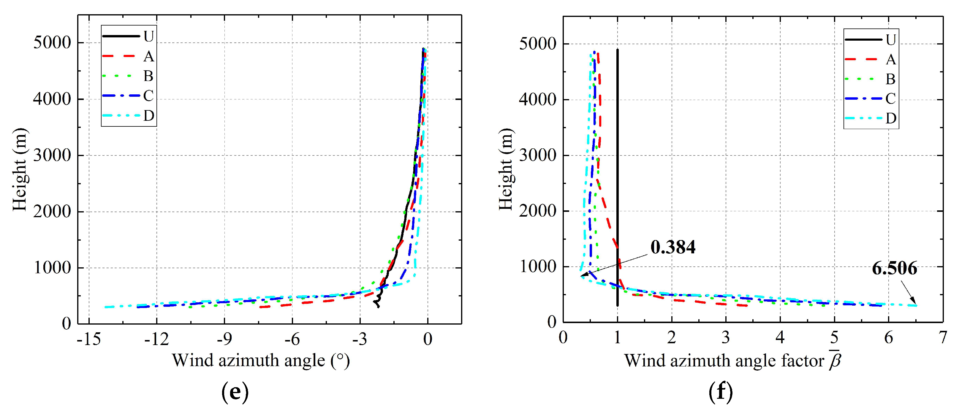
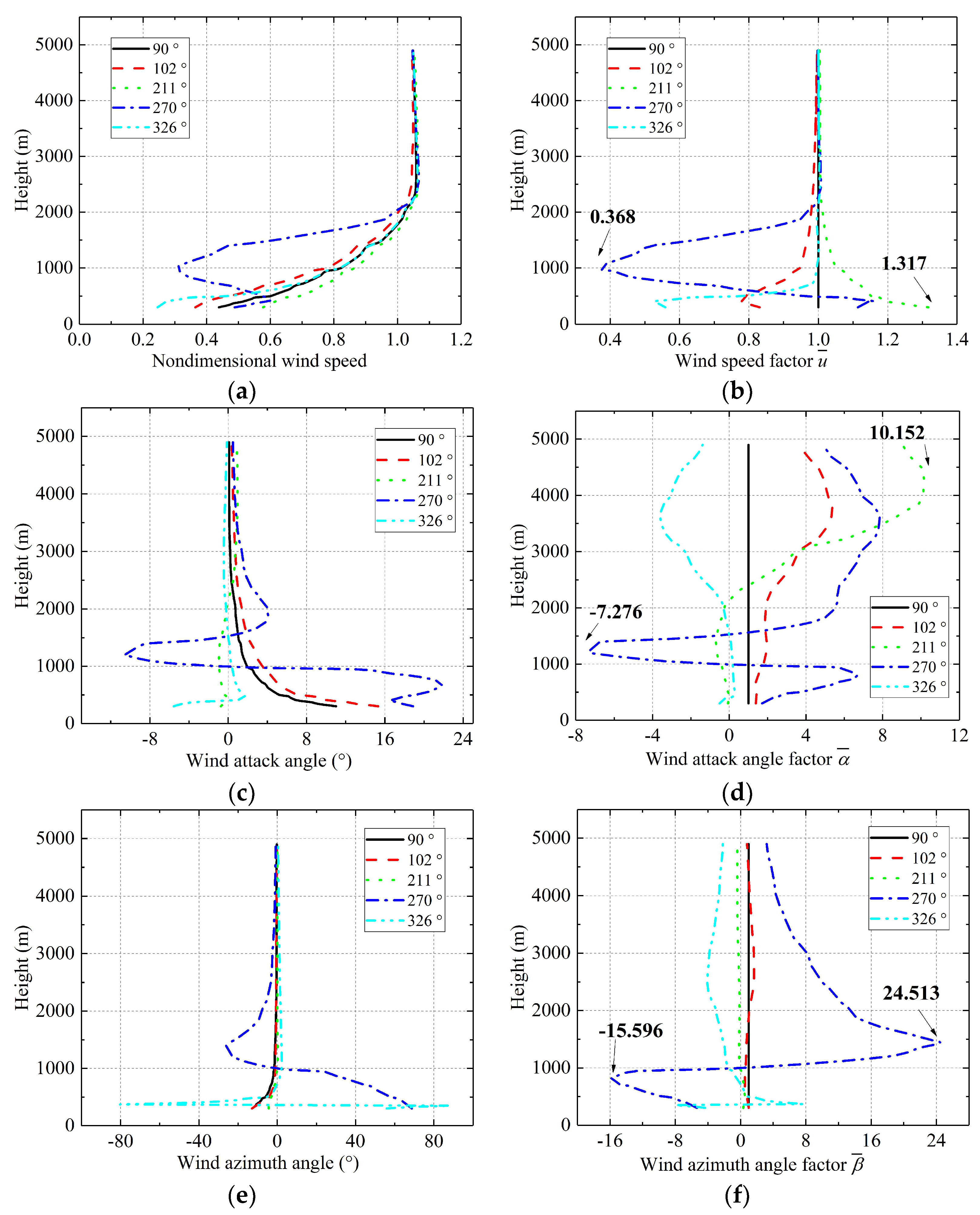
4.1.4. Oncoming Wind Direction

Considering the terrain and climate features of the valley, the oncoming wind direction at the bridge site may be related to the valley extension direction and the dominant wind directions [1,2,17], so three directions along the extension of the valley and two dominant wind directions were designed: 102°, 211°, 326°, 90°, and 270°, as shown in Figure 1a. The surface roughness was set as 0.12 m, and the class C wind speed profile was set at the entrance. The wind speed at the monitoring point was divided by the wind speed at gradient height, and the result is shown in Figure 9.
Then taking the condition with the oncoming wind direction of 90° as the reference condition, and according to Equations (7)–(9), the nondimensional factors were shown in Figure 5b,d,f.
It can be seen from Figure 9 that, compared with the main wind direction of 90° (north wind), the oncoming wind direction had the most obvious influence on the wind parameters. The wind speed factor, wind attack angle factor, and wind azimuth angle factor were much larger than the other initial conditions. Specifically, when the oncoming wind direction was along the valley, the shape of the wind speed profiles was similar: 102°, 211°, and 326°. In addition, due to the limited influence of mountain blocking in this direction, the difference between the main wind direction of 90° and the wind profile of 102° was also not obvious. The most obvious distortion of the wind speed profile occurred in the 270° oncoming wind direction, and the wind speed factor was about 0.4–1.3. When a height of 2500 m was reached, the wind speed profiles tended to be the same. When analyzing the wind speed of a bridge in a valley, it is recommended that more attention is paid to the oncoming wind direction along the valley. The impact of the oncoming wind direction on the wind attack angle and wind azimuth angle is very severe, especially when the oncoming flow is blocked by mountains. According to Figure 9a,c,e and Figure 10b, in the range below 1900 m such as 270°, the oncoming flow was severely blocked by mountains. There was a large wake area, causing the wind speed value at the monitoring point to be significantly lower than the surroundings, the wind direction was distorted, and the wind attack angle and wind azimuth angle fluctuated drastically; the ranges were −10–20° and −90–90°.
The influence of the oncoming wind direction on wind parameters could also be seen from the wind profile and velocity contour shown in Figure 10. It could be found that the oncoming wind direction had an obvious influence on the wind characteristics, especially when the oncoming wind direction was 270°, that is, blocked by the mountains, as shown in Figure 1a and Figure 10b. Therefore, the wind speed, wind attack angle, and wind azimuth angle fluctuated strongly in the low height region such as the height was lower than 2200 m.

4.2. Impact Assessment

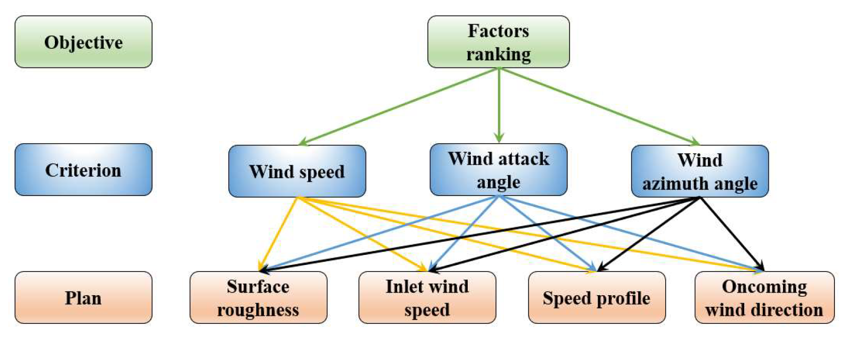
4.2.1. Hierarchical Structure Establishment

In order to study the degree of influence of the initial conditions on wind parameters, the analytic hierarchy process was used to analyze the ranking of factor weights. The ranking of influencing factors was the target level, the wind parameters were the criterion level, and the influencing factors were the scheme level. The hierarchical structure was designed as shown in Figure 11.

4.2.2. Establishment of Quantification Model

In order to link the scale value in the analytic hierarchy process with the numerical results of the wind parameter factors, a quantification model was established. The coefficient of factor sensitivity was defined, which represents the ratio of different wind parameter factors under the same boundary condition, and was used to evaluate the sensitivity of wind parameters. The coefficient of factor sensitivity can be calculated according to Equations (12)–(14):
{ u ¯ , α ¯ , β ¯ } ψ
Δ ψ i = ψ i _ m a x ψ i _ m i n
λ i = Δ ψ i m i n Δ ψ i
where ψ is the wind parameter factor including u ¯ , α ¯ , β ¯ , which are wind speed factor, wind attack angle factor, and wind azimuth angle factor, respectively; ψ i _ m a x and ψ i _ m i n represent the maximum and minimum values, respectively, of the wind parameter factor corresponding to the i th boundary condition, which are marked in Figure 6, Figure 7, Figure 8 and Figure 9; Δ ψ i is the value range of the wind parameter factor; and λ i is the coefficient of factor sensitivity.
Furthermore, the quantification model was used to describe the relationship between the coefficient of factor sensitivity and the scale value in Equation (15), as shown in Figure 12 and Table 4. It could be found that the relationship between the coefficient of factor sensitivity and the scale value represents a logarithmic base 2. The scale value increased with the coefficient of factor sensitivity, but the increase velocity decreased gradually. In other words, as the scale value rises, the corresponding interval of the coefficient of factor sensitivity is sharply augmented.
n = log 2 ( 4 3 ( λ + 1 2 ) )

4.2.3. Impact Assessment Analysis

According to the coefficient of factor sensitivity of various wind parameters and Table 4, the scale value between each layer was drawn, as shown in Table 5. The first five columns of Table 5 consist of an antisymmetric matrix, and the scale value ranged from 1/6 to 6. It could be found that the initial conditions have a huge influence on the distribution of wind parameters.
Using the arithmetic average method to calculate the weights, the data in Table 5 meet the conditions of consistency and also verify the reliability of the quantification model. The final factor weights are shown in Table 6. And the shade of color indicates the size of the weight. The darker the color, the greater the weight.
Using the analytic hierarchy process to study the influence of initial conditions on wind parameters, we can see in Table 6 that for the wind parameters at the mid-span of the bridge in the U-shaped valley, the oncoming wind direction had the greatest influence on the wind attack angle and wind azimuth angle, and the weights were 0.608 and 0.500, respectively; the influence of wind direction and wind profile on wind speed was equivalent, reaching 0.387; and the influence of surface roughness and inlet wind speed on wind parameters was the smallest, not exceeding 0.21. The order of influence is as follows:
(1)
For wind speed: oncoming wind direction = wind speed profile > surface roughness > inlet wind speed.
(2)
For wind attack angle: oncoming wind direction > surface roughness > inlet wind speed > wind speed profile.
(3)
For wind azimuth angle: oncoming wind direction > wind speed profile > surface roughness = inlet wind speed.

5. Conclusions

Influence of the initial conditions on the wind parameters at a bridge middle span in a U-shaped valley by CFD and AHP was investigated in this study. The main conclusions are as follow:
(1)
The numerical results showed that the spatial distribution of wind parameters at the mid-span of a bridge in a U-shaped valley is complex and is significantly affected by the initial conditions.
(2)
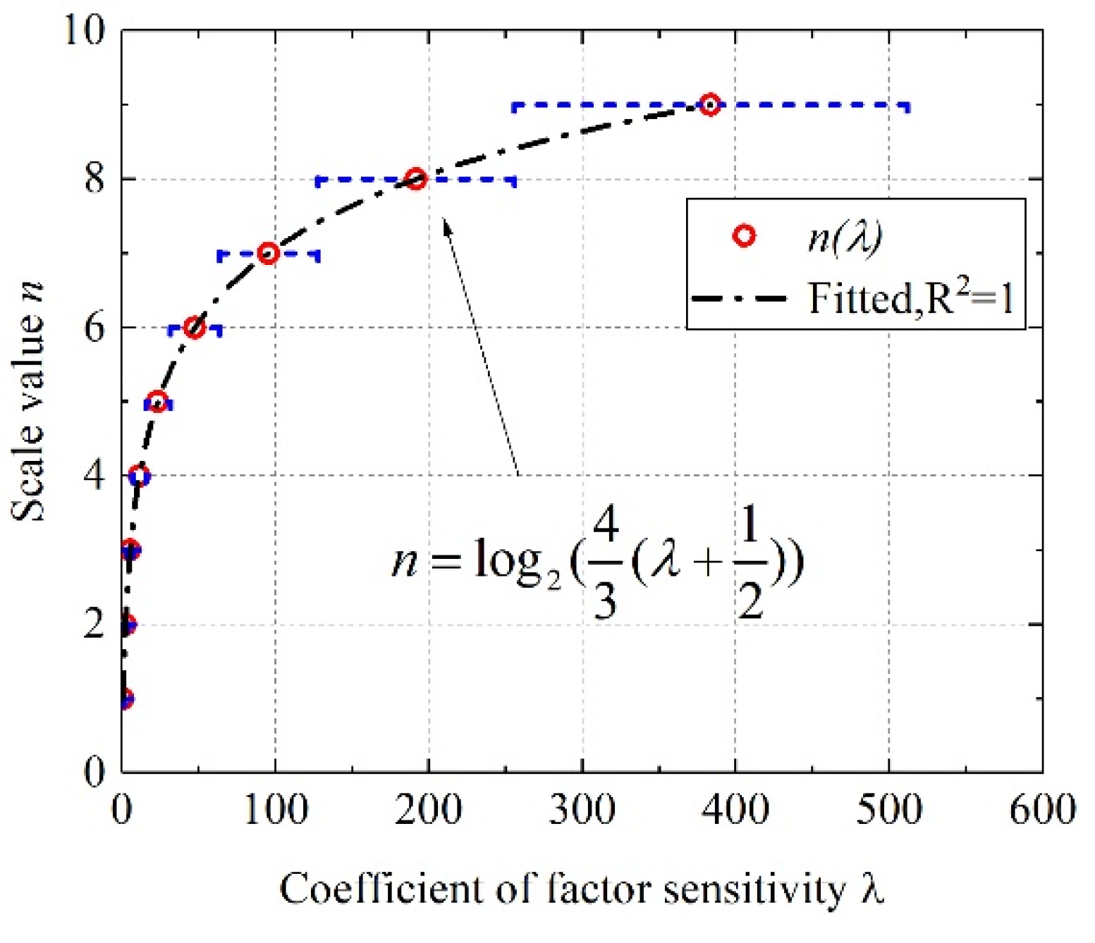
In order to connect CFD and AHP, the wind parameter factor and factor sensitivity coefficient were proposed. A new quantification model was established to describe the functional relationship between the factor sensitivity coefficient and the scale value, and the logarithmic function reliability was verified. An evaluation system for the influence of initial conditions on wind parameters was formed.
(3)
The evaluation results showed that the influence of oncoming wind direction and wind speed profile on wind speed was equivalent, followed by surface roughness and inlet wind speed. The sensitivity of the wind attack angle to the oncoming wind direction was much higher than that of surface roughness, inlet wind speed, and wind speed profile. The oncoming wind direction had the greatest influence on the wind azimuth angle, which was the sum of wind speed profile, surface roughness, and inlet wind speed.
(4)
As for the wind-resistant of bridges in the U-shaped valley, oncoming wind direction was the first initial condition and needs the comprehensive consideration. The second was the wind speed profile. The surface roughness and inlet wind speed were the least important factors.
(5)
This paper did not fully consider the coupling effect of various initial conditions.

Author Contributions

Conceptualization, J.W. and J.L.; Methodology, J.W. and J.L.; Software, J.W.; Validation, J.W., Y.L. and X.Z.; Formal analysis, J.W. and X.Z.; Investigation, J.W. and J.L.; Resources J.W.; Data curation, J.W.; Writing—original draft preparation, J.W.; Writing—review and editing, F.W. and J.L.; Visualization, F.W. and J.L.; Supervision J.L.; Project administration, J.L. and F.W.; Funding acquisition, J.L and J.L. All authors have read and agreed to the published version of the manuscript.

Funding

This work was financially supported by the National Natural Science Foundation of China (51978077) and the Natural Science Basic Research Program of Shaanxi Province (2022JQ-507); the authors would also like to express their gratitude to the sponsors.

Institutional Review Board Statement

The study did not involve humans or animals.

Informed Consent Statement

The study did not involve humans.

Data Availability Statement

No new data were created or analyzed in this study. Data sharing is not applicable to this article.

Conflicts of Interest

The authors declare no conflict of interest.

References

  1. Wang, J.; Li, J.W.; Wang, F.; Hong, G.; Xing, S. Research on wind field characteristics measured by Lidar in a U-shaped valley at a bridge site. Appl. Sci. 2021, 11, 9645. [Google Scholar] [CrossRef]
  2. Wang, F.; Chen, X.M.; He, R.; Liu, Y.; Hao, J.M.; Li, J.W. Wind characteristics in mountainous valleys obtained through field measurement. Appl. Sci. 2021, 11, 7717. [Google Scholar] [CrossRef]
  3. Song, J.-L.; Li, J.-W.; Flay, R.G.J. Field measurements and wind tunnel investigation of wind characteristics at a bridge site in a Y-shaped valley. J. Wind Eng. Ind. Aerodyn. 2020, 202, 104199. [Google Scholar] [CrossRef]
  4. Blocken, B.; van der Hout, A.; Dekker, J.; Weiler, O. CFD simulation of wind flow over natural complex terrain: Case study with validation by field measurements for Ria de Ferrol, Galicia, Spain. J. Wind Eng. Ind. Aerodyn. 2015, 147, 43–57. [Google Scholar] [CrossRef]
  5. Pirooz, A.A.S.; Flay, R.G.J. Comparison of speed-up over hills derived from wind-tunnel experiments, wind-loading standards, and numerical modelling. Bound.-Layer Meteorol. 2018, 168, 213–246. [Google Scholar] [CrossRef]
  6. Chung, J.; Bienkiewicz, B. Numerical simulation of flow past 2D hill and valley. Wind Struct. Int. J. 2004, 7, 1–13. [Google Scholar] [CrossRef]
  7. Braun, A.L.; Awruch, A.M. Finite element simulation of the wind action over bridge sectional models: Application to the Guama river bridge (Para State, Brazil). Finite Elem. Anal. Des. 2008, 44, 105–122. [Google Scholar] [CrossRef]
  8. Li, L.; Zhang, L.-J.; Zhang, N.; Hu, F.; Jiang, Y.; Xuan, C.-Y.; Jiang, W.-M. Study on the micro-scale simulation of wind field over complex terrain by RAMS/FLUENT modeling system. Wind Struct. 2010, 13, 519–528. [Google Scholar] [CrossRef]
  9. Yan, Q.; Peng, Y.; Li, J. Scheme and application of phase delay spectrum towards spatial stochastic wind fields. Wind Struct. 2013, 16, 433–455. [Google Scholar] [CrossRef]
  10. Wang, T.; Cao, S.; Ge, Y. Effects of inflow turbulence and slope on turbulent boundary layers over two-dimensional hills. Wind Struct. 2014, 19, 219–232. [Google Scholar] [CrossRef]
  11. Ren, H.; Laima, S.; Chen, W.-L.; Zhang, B.; Guo, A.; Li, H. Numerical simulation and prediction of spatial wind field under complex terrain. J. Wind Eng. Ind. Aerodyn. 2018, 180, 49–65. [Google Scholar] [CrossRef]
  12. Liu, Z.; He, C.; Liu, Z.; Lu, H. Dimension-reduction simulation of stochastic wind velocity fields by two continuous approaches. Wind Struct. 2019, 29, 389–403. [Google Scholar] [CrossRef]
  13. Lu, X.; Chen, Q.; Qian, C.; Chen, C. Terrain numerical simulation based on RANS/LES hybrid turbulence model. In Proceedings of the 10th International Conference on Environmental Science and Technology, Xiamen, China, 7–9 June 2019; pp. 1–8. [Google Scholar]
  14. Li, J.; Shen, Z.; Xing, S.; Gao, G. Buffeting response of a free-standing bridge pylon in a trumpet-shaped mountain pass. Wind Struct. 2020, 30, 85–97. [Google Scholar] [CrossRef]
  15. Wang, L.; Chen, X.; Chen, H. Research on wind barrier of canyon bridge-tunnel junction based on wind characteristics. Adv. Struct. Eng. 2021, 24, 870–883. [Google Scholar] [CrossRef]
  16. Huang, W.; Zhang, X. Wind field simulation over complex terrain under different inflow wind directions. Wind Struct. 2019, 28, 239–253. [Google Scholar] [CrossRef]
  17. Song, J.-L.; Li, J.-W.; Xu, R.-Z.; Flay, R.G. Field measurements and CFD simulations of wind characteristics at the Yellow River bridge site in a converging-channel terrain. Eng. Appl. Comput. Fluid Mech. 2022, 16, 58–72. [Google Scholar] [CrossRef]
  18. Bakioglu, G.; Atahan, A.O. Evaluating the Influencing Factors on Adoption of Self-driving Vehicles by Using Interval-Valued Pythagorean Fuzzy AHP. In Proceedings of the INFUS 2020: Intelligent and Fuzzy Techniques: Smart and Innovative Solutions, Istanbul, Turkey, 21–23 July 2020; Kahraman, C., Onar, S.C., Oztaysi, B., Sari, I.U., Cebi, S., Tolga, A.C., Eds.; Advances in Intelligent Systems and Computing. Springer: Cham, Switzerland, 2021; pp. 503–511. [Google Scholar]
  19. Chen, Z.-Y.; Dai, Z.-H. Application of group decision-making AHP of confidence index and cloud model for rock slope stability evaluation. Comput. Geosci. 2021, 155, 104836. [Google Scholar] [CrossRef]
  20. Ma, S.; Xu, X.; Chui, J.; Ni, J.; Ma, H.; Tian, H. A New Model to Evaluate Groundwater Vulnerability that Uses a Hybrid AHP-GIS Approach. J. Geol. Soc. India 2021, 97, 94–103. [Google Scholar] [CrossRef]
  21. Merhi, M.I. Evaluating the critical success factors of data intelligence implementation in the public sector using analytical hierarchy process. Technol. Forecast. Soc. Chang. 2021, 173, 121180. [Google Scholar] [CrossRef]
  22. Radhika, E.G.; Sadasivam, G.S. Budget optimized dynamic virtual machine provisioning in hybrid cloud using fuzzy analytic hierarchy process. Expert Syst. Appl. 2021, 183, 115398. [Google Scholar] [CrossRef]
  23. Zadehmohamad, M.; Bazaz, J.B.; Riahipour, R.; Farhangi, V. Physical modeling of the long-term behavior of integral abutment bridge backfill reinforced with tire-rubber. Int. J. Geo-Eng. 2021, 12, 36. [Google Scholar] [CrossRef]
  24. Blocken, B. Computational Fluid Dynamics for urban physics: Importance, scales, possibilities, limitations and ten tips and tricks towards accurate and reliable simulations. Build. Environ. 2015, 91, 219–245. [Google Scholar] [CrossRef] [Green Version]
  25. Huang, G.; Cheng, X.; Peng, L.; Li, M. Aerodynamic shape of transition curve for truncated mountainous terrain model in wind field simulation. J. Wind Eng. Ind. Aerodyn. 2018, 178, 80–90. [Google Scholar] [CrossRef]
  26. Bitsuamlak, G.T.; Stathopoulos, T.; Bédard, C. Numerical evaluation of wind flow over complex terrain: Review. J. Aerosp. Eng. 2004, 17, 135–145. [Google Scholar] [CrossRef]
  27. Hu, P.; Han, Y.; Xu, G.; Li, Y.; Xue, F. Numerical simulation of wind fields at the bridge site in mountain-gorge terrain considering an updated curved boundary transition section. J. Aerosp. Eng. 2018, 31, 04018008. [Google Scholar] [CrossRef]
  28. Hu, P.; Han, Y.; Xu, G.; Cai, C.S.; Cheng, W. Effects of Inhomogeneous Wind Fields on the Aerostatic Stability of a Long-Span Cable-Stayed Bridge Located in a Mountain-Gorge Terrain. J. Aerosp. Eng. 2020, 33, 04020006. [Google Scholar] [CrossRef]
  29. AANSYS. Ansys Fluent User Guide 2019R2; ANSYS. Inc.: Canonsburg, PA, USA, 2019. [Google Scholar]
  30. Pattanapol, W.; Wakes, S.J.; Hilton, M.J.; Dickinson, K.J.M. Modeling of Surface Roughness for Flow Over a Complex Vegetated Surface. In Proceedings of the Conference of the World-Academy-of-Science-Engineering-and-Technology, Bangkok, Thailand, 14–16 December 2007; pp. 273–281. [Google Scholar]
  31. Blocken, B.; Carmeliet, J.; Stathopoulos, T. CFD evaluation of the wind speed conditions in passages between buildings-effect of wall function roughness modifications on the athmospheric boundary layer. J. Wind Eng. Ind. Aerodyn. 2007, 95, 941–962. [Google Scholar] [CrossRef]
  32. Blocken, B.; Stathopoulos, T.; Carmeliet, J. CFD simulation of the atmospheric boundary layer: Wall function problems. Atmos. Environ. 2007, 41, 238–252. [Google Scholar] [CrossRef]
  33. Wieringa, J. Updating the Davenport roughness classification. J. Wind Eng. Ind. Aerodyn. 1992, 41, 357–368. [Google Scholar] [CrossRef]
  34. JTG/T3360-01-2018; Wind-Resistant Design Specification for Hignway Bridges. China Communications Press Co., Ltd.: Beijing, China, 2018.
  35. Zhang, J.; Zhang, M.; Li, Y.; Jiang, F.; Wu, L.; Guo, D. Comparison of wind characteristics in different directions of deep-cut gorges based on field measurements. J. Wind Eng. Ind. Aerodyn. 2021, 212, 104595. [Google Scholar] [CrossRef]
Figure 1. Mesh grid of topographic model. (a) Valley terrain features and oncoming wind direction. (b) Sketch of bridge arrangement.
Applsci 12 04693 g001
Figure 2. Calculation of domain size.
Applsci 12 04693 g002
Figure 3. Grid independence verification. (a) Nondimensional velocity profile. (b) Nondimensional velocity ratio.
Applsci 12 04693 g003
Figure 4. Schematic diagram of grid and boundary.
Applsci 12 04693 g004
Figure 5. Influence of surface roughness on wind parameters: (a) Nondimensional wind speed profile; (b) Nondimensional wind speed factor; (c) Wind attack angle profile; (d) Wind attack angle factor; (e) Wind azimuth angle; (f) Wind azimuth angle factor.
Applsci 12 04693 g005
Figure 6. Influence of inlet wind speed on wind parameters: (a) Nondimensional wind speed profile; (b) Nondimensional wind speed factor; (c) Wind attack angle profile; (d) Wind attack angle factor; (e) Wind azimuth angle; (f) Wind azimuth angle factor.
Applsci 12 04693 g006aApplsci 12 04693 g006b
Figure 7. Wind speed profile of oncoming wind.
Applsci 12 04693 g007
Figure 8. Influence of wind speed profile on wind parameters: (a) Nondimensional wind speed profile; (b) Nondimensional wind speed factor; (c) Wind attack angle profile; (d) Wind attack angle factor; (e) Wind azimuth angle; (f) Wind azimuth angle factor.
Applsci 12 04693 g008aApplsci 12 04693 g008b
Figure 9. Influence of wind direction on wind parameters: (a) Nondimensional wind speed profile; (b) Nondimensional wind speed factor; (c) Wind attack angle profile; (d) Wind attack angle factor; (e) Wind azimuth angle; (f) Wind azimuth angle factor.
Applsci 12 04693 g009
Figure 10. Profile and speed contour: (a) Wind speed profile of different oncoming directions; (b) Wind speed contour at different heights.
Applsci 12 04693 g010
Figure 11. Hierarchical structure diagram.
Applsci 12 04693 g011
Figure 12. Curve of factor sensitivity coefficient and scale value.
Applsci 12 04693 g012
Table 1. Calculation grid.
Grid PrecisionCoarse1Coarse2Middle1Middle2Fine1Fine2
Grid quality2,909,1005,380,4108,050,57511,494,32013,202,82016,131,445
Maximum of the nondimensional velocity ratio1.201.061.061.001.021.01
Table 2. Matrix to judge scale meaning.
Scale ValueDescription
1Two factors are of equal importance.
3When comparing two factors, one is slightly more important than the other.
5When comparing two factors, one is obviously more important than the other.
7When comparing two factors, one is strongly more important than the other.
9When comparing two factors, one is greatly more important than the other.
2,4,6,8Median of two adjacent judgments above.
Inverse If   scale   value   is   a i j when comparing i to j, then   scale   value   is   a j i = 1 / a i j when comparing j to i.
Table 3. Random consistency index ( R I ) value.
n1234567891011121314
RI000.520.891.121.261.361.411.461.491.521.541.561.58
Table 4. Conversion between and coefficient of factor sensitivity and scale value.
Factor Sensitivity Coefficient λ i 0.5~1.51.5~3.53.5~7.57.5~15.515.5~31.531.5~63.563.5~127.5127.5~255.5255.5~
Scale value n 123456789
Table 5. Judgment matrix of the plan level.
(a) Judgment matrix of the initial conditions effect on the wind speed
Wind speedSurface roughnessInlet wind speedWind speed profileOncoming wind direction ψ i _ m i n   ψ i _ m a x Δ ψ i   λ i
Surface roughness122/52/51.00 1.05 0.05 1.52
Inlet wind speed1/211/51/50.97 1.00 0.03 1.00
Wind speed profile5/25110.46 1.01 0.55 17.74
Oncoming wind direction5/25110.37 1.32 0.95 30.61
(b) Judgment matrix of the initial conditions effect on the wind attack angle
Wind attack angleSurface roughnessInlet wind speedWind speed profileOncoming wind direction ψ i _ m i n ψ i _ m a x Δ ψ i λ i
Surface roughness1221/30.69 2.46 1.78 3.24
Inlet wind speed1/2111/60.56 1.17 0.61 1.11
Wind speed profile1/2111/60.80 1.35 0.55 1.00
Oncoming wind direction3661−7.28 10.15 17.43 31.80
(c) Judgment matrix of the initial conditions effect on the wind azimuth angle
Wind azimuth angleSurface roughnessInlet wind speedWind speed profileOncoming wind direction ψ i _ m i n   ψ i _ m a x Δ ψ i λ i
Surface roughness111/31/50.93 2.38 1.45 1.00
Inlet wind speed111/31/50.96 2.48 1.52 1.05
Wind speed profile3313/50.38 6.51 6.12 4.22
Oncoming wind direction555/31−15.60 24.51 40.11 27.64
Table 6. Weight matrix of factors.
Weight
Surface RoughnessInlet Wind SpeedWind Speed ProfileOncoming Wind Direction
Wind speed0.1320.0940.3870.387
Wind attack angle0.2030.1070.0830.608
Wind azimuth angle0.10.10.30.5
Publisher’s Note: MDPI stays neutral with regard to jurisdictional claims in published maps and institutional affiliations.

