
Deep Reinforcement Learning-Based Adaptive Controller for Trajectory Tracking and Altitude Control of an Aerial Robot


School of Mechanical Engineering, Jeonbuk National University, Jeonju 54896, Korea
*
Author to whom correspondence should be addressed.
Appl. Sci. 2022, 12(9), 4764; https://0-doi-org.brum.beds.ac.uk/10.3390/app12094764
Submission received: 14 April 2022
/
Revised: 3 May 2022
/
Accepted: 4 May 2022
/
Published: 9 May 2022
(This article belongs to the Special Issue Robots Dynamics: Application and Control)
Abstract
:This research study presents a new adaptive attitude and altitude controller for an aerial robot. The proposed controlling approach employs a reinforcement learning-based algorithm to actively estimate the controller parameters of the aerial robot. In dealing with highly nonlinear systems and parameter uncertainty, the proposed RL-based adaptive control algorithm has advantages over some types of standard control approaches. When compared to the conventional proportional integral derivative (PID) controllers, the results of the numerical simulation demonstrate the effectiveness of this intelligent control strategy, which can improve the control performance of the whole system, resulting in accurate trajectory tracking and altitude control of the vehicle.
1. Introduction
1.1. Control Problem of Aerial Robots
Aerial robots have become increasingly popular in recent decades. Quadrotors, in particular, have piqued the attention of the scientific community, with several important discoveries and applications proposed and tested. Despite significant advancements, aerial robot control is still regarded as a very active field of research. Aerial robot controllers, on the one hand, need the ability to acquire, process, and calculate forces to apply to vehicle actuators in a very time-critical way. The flight controllers for aerial robots, on the other hand, should be able to resist failures and respond to changes in payload and disturbances. Flight control systems for aerial robots are usually implemented using proportional integral derivative (PID) control algorithms [1]. PIDs have proved their acceptable performance in some circumstances, such as racing drones, where fast control responses are crucial. A PID controller works close to optimally in stable settings and environments. Hence, most commercial aerial robot flight controllers use PIDs for both attitude and altitude control.
However, PID controllers are unable to properly control a robot when faced with unexpected dynamics disturbances (such as variable payloads) [2,3,4,5,6,7,8,9,10,11,12]. External disturbances (e.g., wind) can also reduce the accuracy of trajectory tracking by weakening attitude controller performance. The problem is that model-free controllers are unable to fully cover the complicated variations in nonlinear dynamics behavior of a quadrotor, causing the controller to lose stability and robustness [13]. This problem motivated some researchers to develop optimal and nonlinear model-based controllers to control aerial robots. Nonlinear Model Predictive Control (NMPC) is one of the most widely used optimal model-based control algorithms in many recent research works. The controller, as the name implies, uses a model of the system to forecast the future behavior of the robot in response to the current control input. A model predictive controller has some advantages over its model-free counterparts. Not only does the controller outperform its model-free equivalents in terms of control performance, but it also has the ability to take into account some constraints, which is a key element in some flight maneuvers such as obstacle avoidance [14]. Despite its benefits over previous model-free techniques, MPC is vulnerable to failure when the prediction model of the controller does not account for fluctuations in the dynamical system under control.
When it comes to controlling an aerial robot, it should be noted that the aerial robot controller needs to control both the altitude and the attitude of the robot. In order to implement a full optimal model-based controller for an aerial robot, some researchers proposed employing NMPC for both altitude and attitude controllers, while taking some measures to reduce its dependency on an accurate model of the robot. Some studies endeavored to mitigate the problem by using learning algorithms (e.g., a Gaussian process or neural networks) that actively estimate the dynamics parameters of the robot and update the prediction model in real time [15,16,17,18,19,20]. Although the resultant topologies improved the performance of the controller after learning the dynamical variations of the system, the methods have the potential to increase computation costs.
Despite the fact that the aforementioned optimal control algorithms partially managed to improve the overall performance of controllers, they need powerful and fast processors to compute the online optimization problem. In order to avoid imposing high computing costs on the system, a number of research studies proposed using linear model predictive control (LMPC) [21,22,23]. The advantage of LMPC is its low computation cost, as compared with its nonlinear counterpart. The controller, however, does not provide a good response for attitude control when there is too much variation in the parameters of the dynamical system. The problem stems from the fact that the prediction model in the linear MPC uses a linearized model around its ideal working point. The linearized model, however, is not sufficient to be used as a prediction model for the attitude control of aerial robots that need to do challenging maneuvers. Although the LMPC is not an ideal controller for attitude control, it is sufficient for altitude control, because most aerial robots fly at low altitudes with limited variation in elevation; thus, the linearized model around that working altitude can cover the behavior of a flying robot [24,25].
Although PID controllers cannot fully cover fluctuations in system dynamics, they provide fast control response, which is a crucial ability for an aerial robot that requires agile attitude control responses to avoid obstacles and perform demanding maneuvers (e.g., delivery aerial robots in urban areas) [26]. In previous research efforts, many researchers have explored a variety of techniques to mitigate the problem in conventional standard PIDs. Several studies combined online tuning approaches with PID control to lessen the impact of changes in vehicle dynamics and disturbances [27]. A number of researchers opted for training neural networks to actively update the PID gain values of aerial drone controllers [28,29]. However, neural network training needs a large database of labeled data. Another widely used approach to actively tune the PID control is the fuzzy-logic-based auto-tuning algorithm [30,31,32]. The drawback of the fuzzy-logic-based tuning strategy is that the efficiency of algorithm is strongly reliant on the fuzzy rules and the inference system set by the designer. However, some fluctuations in the system dynamics may be unanticipated, resulting in the generation of inaccurate control gain coefficients by the fuzzy logic [33].
In addition to the aforementioned optimal control and active tuning approaches (for PIDs), Reinforcement Learning (RL) and Deep Reinforcement Learning (DRL) are other new approaches that have recently made their way into the field of aerial robots control. RL and DRL do not require an accurate model of the plant under control or human designed control rules, in contrast to fuzzy logic that depends on the expert’s expertise. As a result, these machine learning approaches have attracted the attention of many academics working on the control of systems with uncertain dynamical models [34,35,36]. Unlike neural network-based control techniques, deep reinforcement learning does not require large labeled datasets. This is a major benefit, since labelling data for all critical scenarios become more and more expensive as the number of required data grows. Another important advantage of deep reinforcement learning for control is its capability to directly map image features to control states, thereby resolving the need for the implementation of complex state estimators and image processing algorithms in some special cases [37].
1.2. Related Works
Some researchers have already applied RL algorithms to control aerial robots. However, the bulk of studies focused on directly using RL algorithms to control aerial robots. As an example of these efforts, in a research study published in [38], a deep reinforcement learning algorithm was employed to control a fixed-wing aerial robot. The nonlinearities of the dynamics model, as well as the coupling effect between lateral and longitudinal control, were taken into account in the mentioned research study. The Proximal Policy Optimization (PPO) is the RL algorithm utilized in the study. Similarly, another research paper [39] employed PPO to regulate the attitude of a quadcopter. A research study presented in [40] employed a control system to achieve accurate autonomous driving of an aerial vehicle while landing on a platform. In the latter research paper, the Deep Q-learning Network (DQN) is the cornerstone of the controlling approach to mapping the images of poor quality to control states. Although the DQN method appears to be a promising approach for tackling vision-based control problems, it has significant drawbacks that limit its usage in more advanced vehicle control tasks that rely on image processing. As another example of this series of research efforts, a research study published in [41], leveraged an RL-based approach to control an aerial robot with the objective of capturing photographs of a person’s front view, particularly his face. RL-based controllers also have found their ways into the world of morphing aerial robots. For instance, a work presented in [42] used a combination of the PPO algorithm with a PID controller to control a morphing aerial robot.
In contrast to the majority of the mentioned works that used RL algorithms to directly control aerial robots, some researchers opted not to use RL for that purpose. Instead, some attempts have been made to use the RL-based algorithm as a foundation for active tuning and state estimation mechanisms for other classical controllers. The drawback of a direct RL-based control algorithm is its slow response, compared with that of conventional PID controllers that provide very fast controlling responses [43]. In addition, direct deep reinforcement learning-based controlling approaches does not provide any analytical guarantees for the stable response and robustness in the control process, as unexplainable neural networks underpin its structure. However, RL has the potential to be used along with traditional control algorithms to provide adaptive and robust controllers.
As an example of the latter approach, the research study reported in [44] employed a fault-tolerant RL-based adaptive controller that combined an RL-based adaptive algorithm (in the study PPO) with a PID controller and an Unscented Kalman Filter (UKF) to develop a fault-tolerant RL-based adaptive controller. The proposed controlling strategy has employed a hybrid of parameter estimation and a deep reinforcement learning method. When the value of the parameters associated with faults affected the controller performance, the algorithm updated the PID controller. Although the findings of the study revealed a satisfactory control response for altitude control, the attitude control response did not provide clear superiority over earlier conventional controllers. Another research study [45] developed an adaptive neuro-fuzzy PID controller for nonlinear systems based on the Twin Delayed Deep Deterministic Policy Gradient (TD3) method. The observation of the environment is integrated with information from a multiple-input single-output (MISO) fuzzy inference system (FIS) and has a specifically defined fuzzy PID controller functioning as the actor in the TD3 method, which provides automated tuning of fuzzy PID controller gains.
1.3. Research Objectives
The majority of the aforementioned research studies focused solely on improving either attitude control performance or altitude controller response. In addition, it must be noted that some DRL algorithms are more efficient for attitude control (e.g., PPO), while another group of DRL algorithms (e.g., DDPG) shows better performance in improving trajectory tracking [46]. In order to compensate for fluctuations in the dynamics of the aerial robot, in the proposed controlling architecture, a reinforcement learning algorithm interacts with the system and learns adaptation policies for actively updating the gains of the controllers. To adjust the parameters of the attitude PID controller, the trained policy actively creates appropriate control gain values. Similarly, the scaling factor of the compensator is updated using actions generated by the RL agent. The aerial RL-based adaption algorithm is trained in a simulated environment in MATLAB software.
The rest of this paper is organized as follows: In Section 2, the dynamic model of a quadrotor is discussed. In Section 3, the control problem of the aerial robot is addressed, where the altitude and attitude control of the robot is discussed before introducing the proposed RL-based adaptive control framework. The applicability and efficacy of the proposed control strategy are evaluated in a simulated environment in Section 4. Finally, Section 5 summarizes the research findings.
2. Aerial Robot Dynamics
The aerial robot used in this research study is a quadcopter. Quadcopters are substantially underactuated, with six degrees of freedom (three translational and three rotational) and only four distinct inputs (rotor speeds). Rotational and translational motions are coupled to achieve six degrees of freedom. After accounting for the intricate aerodynamic effects, the resulting dynamics is highly nonlinear. As another property of quadcopters, it must be noted that, unlike conventional helicopters, the rotor blade pitch angle in a quadcopter does not need to be varied.
2.1. Quadcopter Coordinate Frames, Forces, and Torques
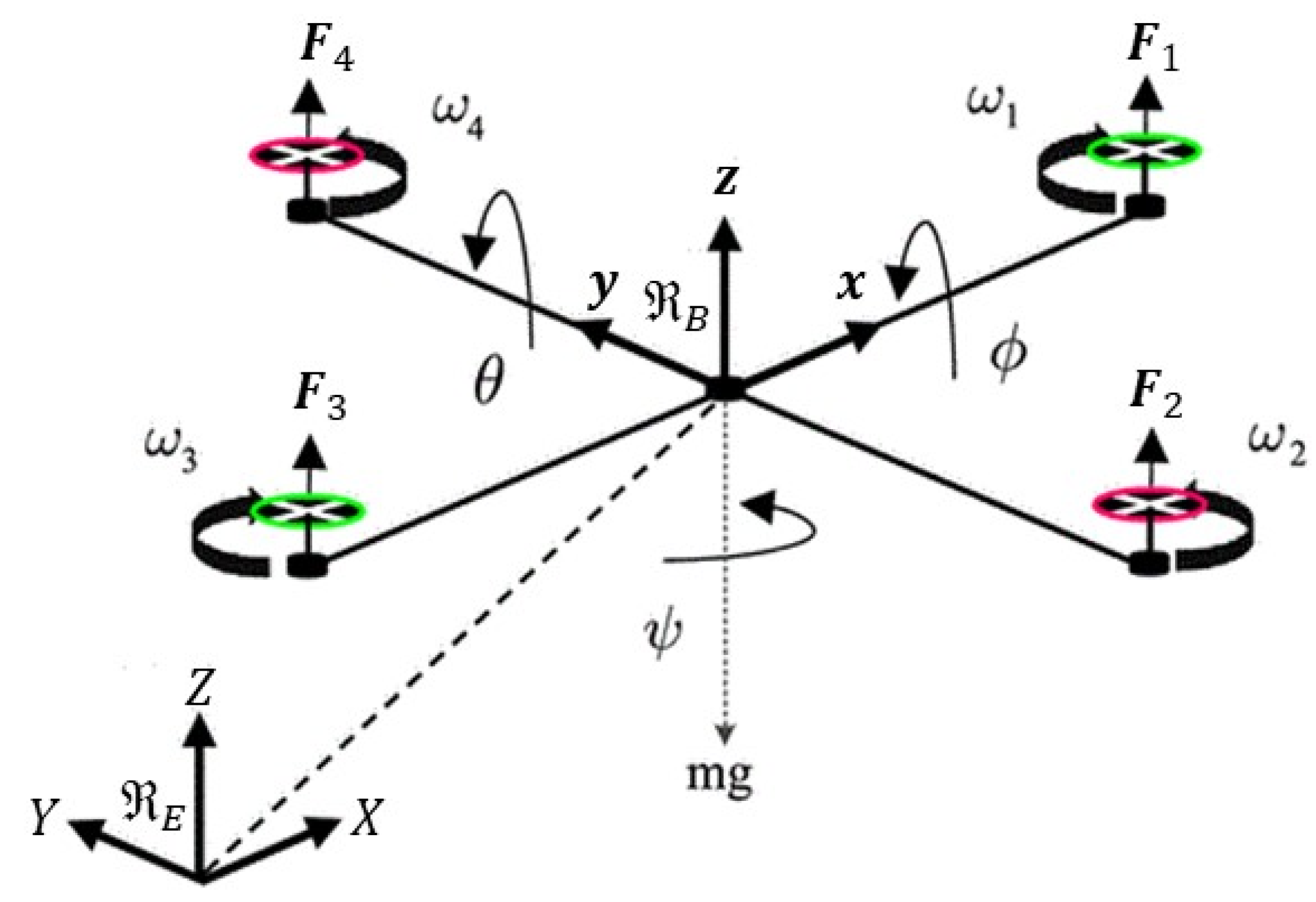
The reference coordinate frame and the coordinate frame of the vehicle body must be determined before building a mathematical model of the quadrotor, as shown in Figure 1. The ground and the reference coordinate frames are both tied to . The is a coordinate frame that is attached to the body of the vehicle and has its center aligned with the center of mass of the robot.
In this research study, the dynamical equations governing the quadcopter were derived from the text published in [47]. The following assumptions were taken into consideration in order to determine the examined equations of the motion of the system:
- The aerial robot consists of a stiff body with a symmetrical structure.
- The geometrical center of the robot is the same as its center of gravity and mass.
- The moment of inertia of the propellers has been overlooked.
The dynamical model of the system could be constructed by taking into account both the translational dynamic (Newton’s second law) and the rotational dynamic (Euler’s rotation equations).
2.2. Translational Dynamics
The following forces acted on the system being studied:
- The total weight of the vehicle, as expressed in Equation (1).
- The generated thrust of rotors, which can be calculated using Equation (2).
- As indicated in Equation (3), the drag force and air friction.
In the equations, the gravity acceleration is denoted by . In Equation (2), the Euler angles are represented by (. The rotation transform matrix, the angular velocity of the th propeller, and the thrust constant are represented by R,, and b, respectively. In Equation (3), is the matrix of translational drag coefficients. The position of the center of mass (ξ) in the flat earth coordinate is defined as a 3 by 1 vector. The equation of motion that describes the translational motion of a quadcopter can be stated as follows, using Newton’s second law:
2.3. Rotational Dynamics
A quadrotor is affected by roll, pitch, and yaw torques, as well as by an aerodynamic friction torque and the gyroscopic effect of the propeller. The torques are expressed as follows, in Equations (8)–(12):
where is the distance between the motor axis and the center of mass of the quadcopter. In Equation (11), is a 3 by 3 matrix of aerodynamic friction coefficients. In Equation (12), and , respectively, are the inertia and rotation velocity of rotors. Applying Euler’s rotation equations yields the equations of motion (Equations (13)–(15)) that govern the rotating motion of the quadrotor. In the equations, are moments of inertia along the directions respectively:
2.4. Dynamics Model of the Quadcopter
Having considered both translational and rotational dynamics, the entire dynamic model of the quadcopter could be stated as follows:
where is a vector expressed as follows (in the equations, is the drag coefficient):
3. Quadcopter Control
3.1. Controller Framework
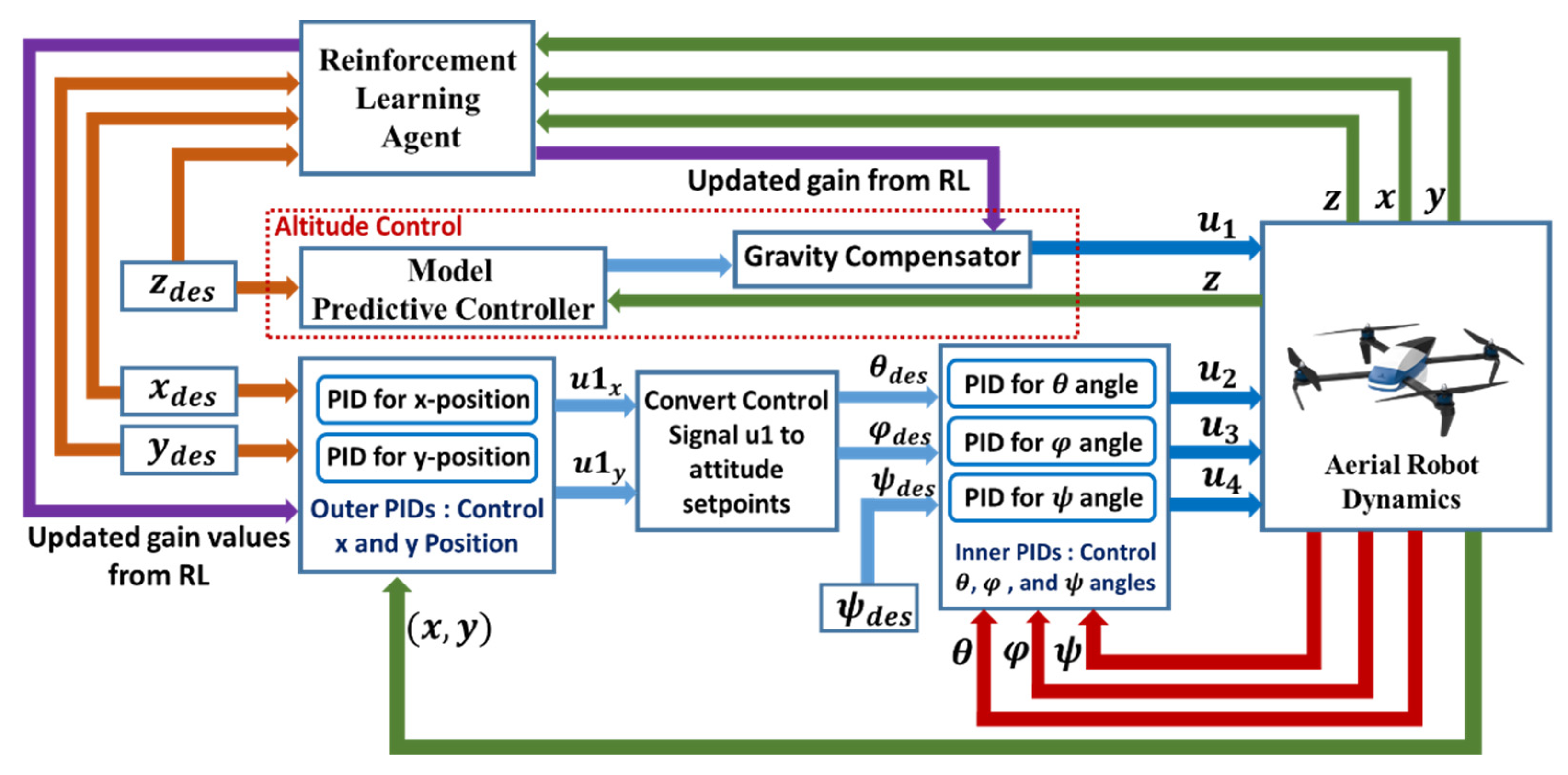
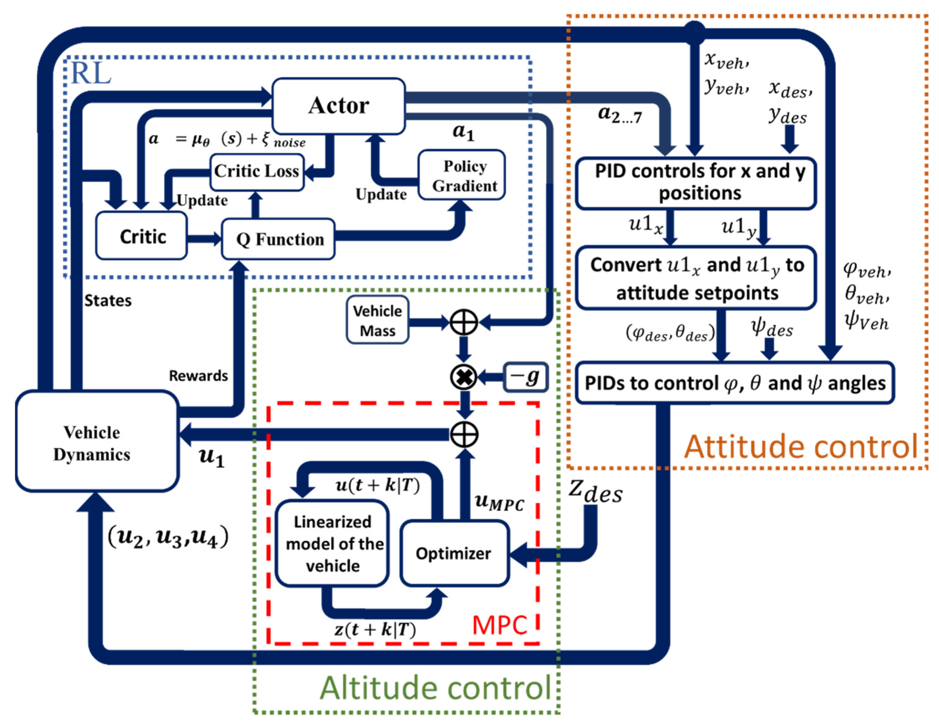
A quadcopter is an underactuated system, which means that six degrees of freedom in space are controlled by just four motors. Hence, controllers in such vehicles must be designed for a subset of four degrees of freedom. Furthermore, the fact must be taken into account that the control of the x and y positions in space is influenced by changes in the pitch and roll angles. Having considered the aforementioned relationships, the control of a quadrotor is normally designed for two independent subsets of coordinates. The necessity for a swashplate mechanism is eliminated with four separate rotors. The swashplate mechanism was necessary to give the helicopter more degrees of freedom, but the same level of control can be achieved by simply adding two more rotors, as implemented in the structure of quadcopters. Despite the fact that the command is for three position coordinates (x, y, z) plus yaw angle, the control algorithm employs both roll and pitch orientation controllers. In the inertial coordinate system, the control signals of three position controllers define a force vector (thrust). The setpoints () transmitted to the roll and pitch controls are considered as the orientation of the vector. The stated architecture, as well as the elements of our proposed controllers, are depicted in Figure 2, which will be explored in the next sections.
The altitude controller and the attitude controller are the two main parts of the control architecture. The altitude controller, as shown in Figure 2, maintains the altitude of the aerial robot at the required level. In most commercial aerial robots, the altitude controller is a PID controller with fixed control gain values. In this research, a proposed control architecture consisting of a MPC controller and a gravity compensator is proposed as a replacement for conventional PID controllers. The scaling factor of the compensator is adaptively adjusted during the operation of the robot, using actions generated by the reinforcement learning agent. The robot attitude controller is the second major controlling component of the system. The controller is made up of two distinct PID controller blocks. The difference between the desired x and y position and the actual x and y location in space is measured and defined as the position error in 2D. The x-position and y-position PID controllers in the outer loop were designed to minimize the error. The control commands of the position controllers are transformed to appropriate roll and pitch setpoints. The inner loop PID controllers use the resulting roll and pitch setpoints as reference inputs. The control gain values of the inner loop PID controllers are constant in our proposed control architecture, whereas the control gain values of the outer loop PID controllers are adaptively adjusted using trained policy from the RL-based adaptation algorithm.
3.2. Attitude Control
To control the attitude of the robot, an architecture comprising of RL-based adaptive controllers is proposed in this study. The outer loop PID controllers were designed to generate the and virtual control signals as described in Equations (25)–(28). Equation (29) is used to convert the control commands from outer loop PIDs to the necessary roll and pitch reference values for the inner-loop PID controllers.
As indicated in Equations (30)–(32), three PID controllers were implemented in the inner loop PID control block to provide manipulated variables for robot attitude control.
The optimal control gains for the inner loop PID controllers were obtained, based on several trials and errors. The obtained gain coefficients are listed in Table 1. The control gains of outer loop PID controllers are actively estimated and adjusted by the RL agent.
3.3. Altitude Control
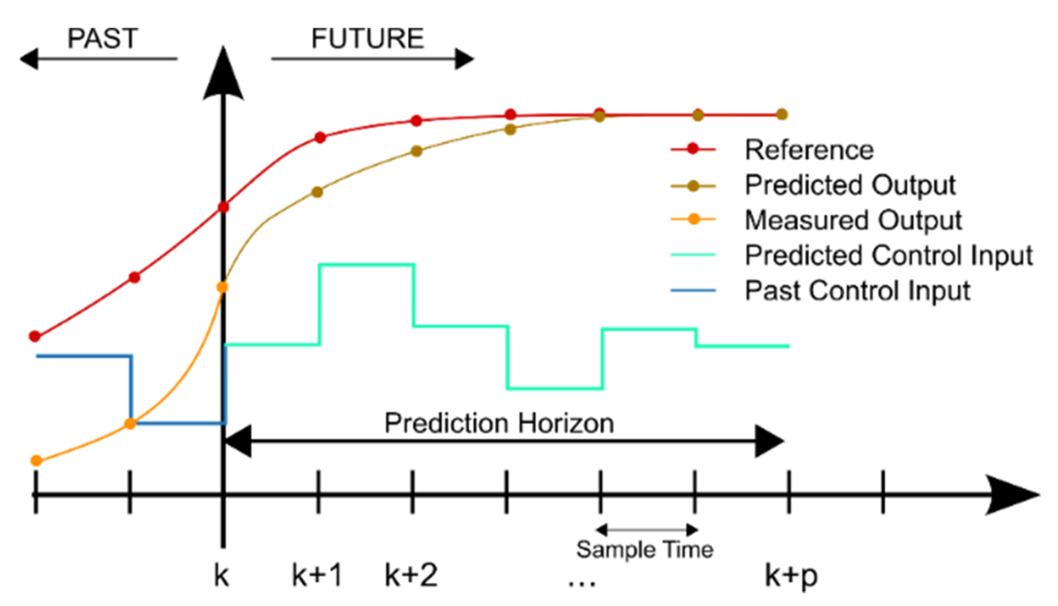
In this study, the proposed altitude controller utilizes a linear model predictive controller and a gravity compensator in its controlling architecture. The gravity compensator is responsible for alleviating the effect of forces that arise from fluctuations in the weight of the robot. The scaling factor of the compensator is adaptively updated using the RL policy. The proposed algorithm aimed to mitigate the impact of disturbances arising from changes in the weight of the robot on the performance of the aerial robot in trajectory tracking and altitude stabilization. The MPC is based on an iterative, finite-horizon robot model optimization. The present states of the quadcopter are sampled at time t, and a cost-minimizing control strategy for a relatively short time horizon in the future is computed (using a numerical minimization technique). At each control interval, model predictive control solves an optimization problem, a quadratic program (QP). Until the next control interval, the solution generated a sequence of manipulated variables to be applied to the robot. A series of online optimizations are run to estimate possible state trajectories that would arise from the present states. Furthermore, the solution identifies a cost-minimizing control strategy (by the solution of Euler–Lagrange equations) from t until time ran out at t + T. Although the MPC computes a series of manipulated variables, only the first step of the computed control strategy is applied to the quadcopter, after which the updated states of the robot are sampled again and the computations are repeated using the updated states, resulting in computation of fresh control inputs and a new anticipated state route. Figure 3 shows the relationship between the prediction horizon and generated control inputs.
Model predictive control is considered as a multivariable controlling algorithm incorporating the following components:
- A dynamics model of the system under control.
- A cost function J.
- An optimization mechanism. The optimal manipulated variable () is computed by minimizing the cost function J using the optimization algorithm.
A typical cost function in the MPC algorithm is made up of four terms, each of which focuses on a different element of controller performance (k represents the current control interval):
where dk signifies optimal control inputs that are obtained by solving a quadratic programming (QP) problem, as indicated in Equation (34). In Equation (33), JRT(dk) is reference tracking cost. Here, Ju(dk) and JΔu(dk) are representations of manipulated variable tracking and manipulated variable move suppression, respectively. The last cost term in Equation (33), JΔu(dk), decreases the control effort, thereby reducing the energy consumption of the actuators (e.g., the dc motors of the quadrotor). The MPC cost function can be formulated as follow:
In Equation (35), is a () weight matrix ( is the number of plant output variables). Here, and () are positive-semi-definite weight matrices ( represents the number of manipulated variables). In the aforementioned cost function, p is the prediction horizon, which can be adjusted according to the controller performance and the processing power of the hardware. In Equation (35),, , and can be computed, using Equations (36)–(38).
The reference value (or reference values) given to the controller at the th prediction horizon step is specified as . Similarly, the value (or values) of outputs variables of the plant, sampled at the th prediction horizon step, is defined as . In the equation, reflects the value (or values) of desired control inputs corresponding to . In the proposed MPC control architecture, in this paper, there is one manipulated variable, . In addition, in this paper, is the altitude (z position) of the robot, while is the desired altitude for the robot. In order to reduce the controller effort and alleviate the effects of arising fluctuations in the weight of the aerial robot, this study proposed to use a gravity compensator after the MPC controller. The final altitude control input is defined as:
In Equation (39), is the scaling factor of the compensator that is actively estimated by the RL policy. In order to evaluate the performance of the proposed control architecture in controlling an aerial robot, a dynamics model of a commercial aerial robot named Parrot was chosen and implemented in the simulator environment as the aerial robot under control. The dynamics model specifications of the employed Parrot quadcopter are listed in Table 2.
This research study employs a linear model predictive control. Hence, a linear state-space model of the quadcopter is required. Equation (40) describes the standard form of a linear time-invariant (LTI) state-space model, which has p inputs, q outputs, and n state variables.
where x, y, and u are the state vector, the output vector, and the input vector, respectively. In the equation, A, B, and C are (), the state matrix; (), the input matrix; and (), the output matrix, respectively. It should be noted that D is a () feedforward matrix. The D matrix is zero in this study, as there is no direct feedthrough. The linear model was computed around the operational point in the state-space model using the MPC Designer app in the Model Predictive Control Toolbox. The toolbox included in the MATLAB software provides control blocks for developing not only linear model predictive control but also nonlinear and adaptive model predictive controllers. In addition, the MPC Designer app included in the software package facilitates the design of an LMPC by automating the processes for plant linearization and tuning the controller parameters. The state-space parameters of the linearized plant can be found in the MPC object (MPCobj) generated by the MPC Designer app. The Simulink MPC Designer linearizes each block in the model independently, then combines the outputs of the individual linearized models to produce the linearized model of the whole plant. Table 3 presents the resulting values for the state-space model generated by the app.
3.4. Deep Reinforcement Learning for Online Parameter Estimation and Tuning
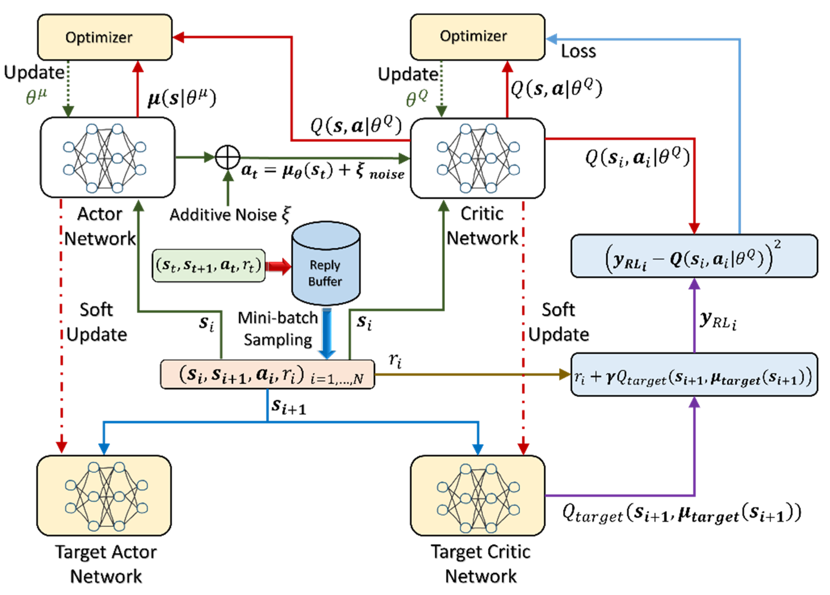
The proposed parameter estimation approach in the study utilizes a DRL algorithm to actively estimate and adjust the parameters both in PID controllers and the compensator. A reinforcement learning agent was developed in the Simulink environment to construct an adaption topology for actively estimating the tuning parameters of the designed controllers. In the first stage, the reinforcement learning algorithm interacted with the dynamics model of the robot (in the simulator environment) to learn the appropriate tuning rules. During the operation time of the robot, the trained policy is used to actively adjust the gain values of the controllers. In this study, the RL algorithm is the Deep Deterministic Policy Gradient (DDPG). The DDPG is an approach that combines the idea from DPG with the Deep Q-learning Network (DQN) to create an off-policy algorithm that is able to work with continuous action space [49]. It aims to generate the optimal action policy for the agent to maximize rewards while fulfilling its objectives [50]. The DDPG algorithm can work over continuous action spaces, which is a significant challenge for traditional RL approaches such as Q-learning. The DDPG algorithm is a hybrid technique that incorporates both the policy gradient and the value function. The architecture of DDPG is based on the actor-critic framework. In the algorithm, the actor refers to the policy function, whereas the critic refers to the value function Q. The critic network evaluates the actions of the actor based on the rewards and the subsequent state resulting from the environment. The role of the critic is to adjust the weights of the actor network so that the future actions of the actor result in the highest potential cumulative reward. The goal in the DDPG algorithm is to learn a parameterized deterministic policy , such that the obtained optimal policy maximizes the expected reward over all states reachable by the policy:
where is the distribution of all states reachable by the policy. It is proven that maximizing the returns or true Q-value of all actions leads to the same optimal policy. This is an idea introduced in dynamic programing, where policy evaluation first finds the true Q-value of all state-action pairs, and policy improvements change the policy by selecting the action(s) with the maximal Q-value:
in Equation (42), is the action(s) with maximal Q-value. The action is expected to generate the maximum expected reward. In the continuous space, the gradient of objective function can be considered to be the same a as the gradient of the Q-value. If we have an estimate of all the value of any action (), changing the policy in the direction of leads to an action with higher Q-value and associated return:
In Equation (43), gradient with regard to action of the Q-value is taken. We can expand the above equation by applying the chain rule.
To obtain an unbiased estimate of the Q-value of any action and compute its gradient, it is possible to calculate a function approximator , as long as it is compatible, and to minimize the quadratic error with the true Q-values:
The goal of the DDPG algorithm was to extend the DPG to incorporate non-linear function approximators. The objective was fulfilled by combining DQN and DPG concepts to create an algorithm working over continuous space. Furthermore, the following elements were added to the base DPG algorithm.
- An experience reply memory to store past transitions and learn off-policy.
- Target networks to stabilize learning.
DDPG updates the parameters of target networks after each update of the trained network using a sliding average (soft update) for both the actor and the critic:
where is a hyperprameter between 0 and 1. The modified update rule guarantees that the target networks are always lagging behind the trained networks, providing more stability to the learning of Q-values. The key idea borrowed from DPG is the policy gradient for the actor. The critic is learned using regular Q-learning and target networks:
where is the value of the action that is estimated to return the largest total future reward, based on all possible actions that can be made in the next state. In the Equation (49), is the discount factor. Noise is added to improve exploration:
The additive noise is an Ornstein–Uhlenbeck process that generate temporally correlated noise with zero mean. The target value can be computed using the target network:
The following loss function is minimized, resulting in an update in the critic. A sampling policy gradient can also be applied to update the actor:
Figure 4 depicts the aforementioned learning process in the DDPG algorithm. The architecture is comprised of two actor-critic networks. The target networks in the architecture stabilized the learning procedure. The noise improves the exploration of the reachable control states. The proposed RL-based control algorithm (Algorithm 1) is described in the following pseudocode.
| Algorithm 1. The proposed algorithm. | |||||
| 1: | Initial policy network and critic network with weights respectively. | ||||
| 2: | Set target policy network and target critic network with weights | ||||
| 3: | Set target parameters weights equal to main parameters weights: | ||||
| 4: | for episode = 1, M do | ||||
| 5: | Initialize a random process noise for action exploration. | ||||
| 6: | Receive initial observation state . | ||||
| 7: | for t = 1, T do | ||||
| 8: | Select actions where | ||||
| 9: | Observe a vector of states s | ||||
| 10: | Apply actions ( to outer loop PID controllers as follow: | ||||
| 11: | Use the updated and to generate | ||||
| 12: | Use as setpoints for inner loop PIDs and generate , and . | ||||
| 13: | Compute by minimizing the MPC cost function. | ||||
| 14: | Compute using the generated namipulated variable from MPC and the scalling factor of the compensator ) | ||||
| 15: | Apply control inputs ,, and to the drone dynamics model. | ||||
| 16: | Observe the next vector of states , and the next reward r | ||||
| 17: | Store () in reply buffer D. | ||||
| 18: | Randomly sample a minibatch of N transitions () from D. | ||||
| 19: | Compute targets: | ||||
| 20: | Update critic by minimizing the loss: | ||||
| 21: | Update the actor policy using a sampled policy gradient: | ||||
| 22: | Update the target networks: | ||||
| 23: | | ||||
| 24: | end for | ||||
| 25: | end for | ||||
The actor outputs are actions () selected from a continuous action space by considering the current state of the environment. In this study, the action is comprised of a vector of actions . Here, are used to actively estimates and tune the gain coefficients of the outer loop PID controllers for x and y positions, which are two controllers located in outer loop PID control block. The action ( generates an updated estimation of the proper scaling factor for updating the compensator. The defined states were errors and . The Q function is computed using the rewards from the environments. The notion is that the best policy can be found by maximizing the true Q-value of all actions. The architecture of the proposed adaptive RL-based controller is shown in Figure 5.
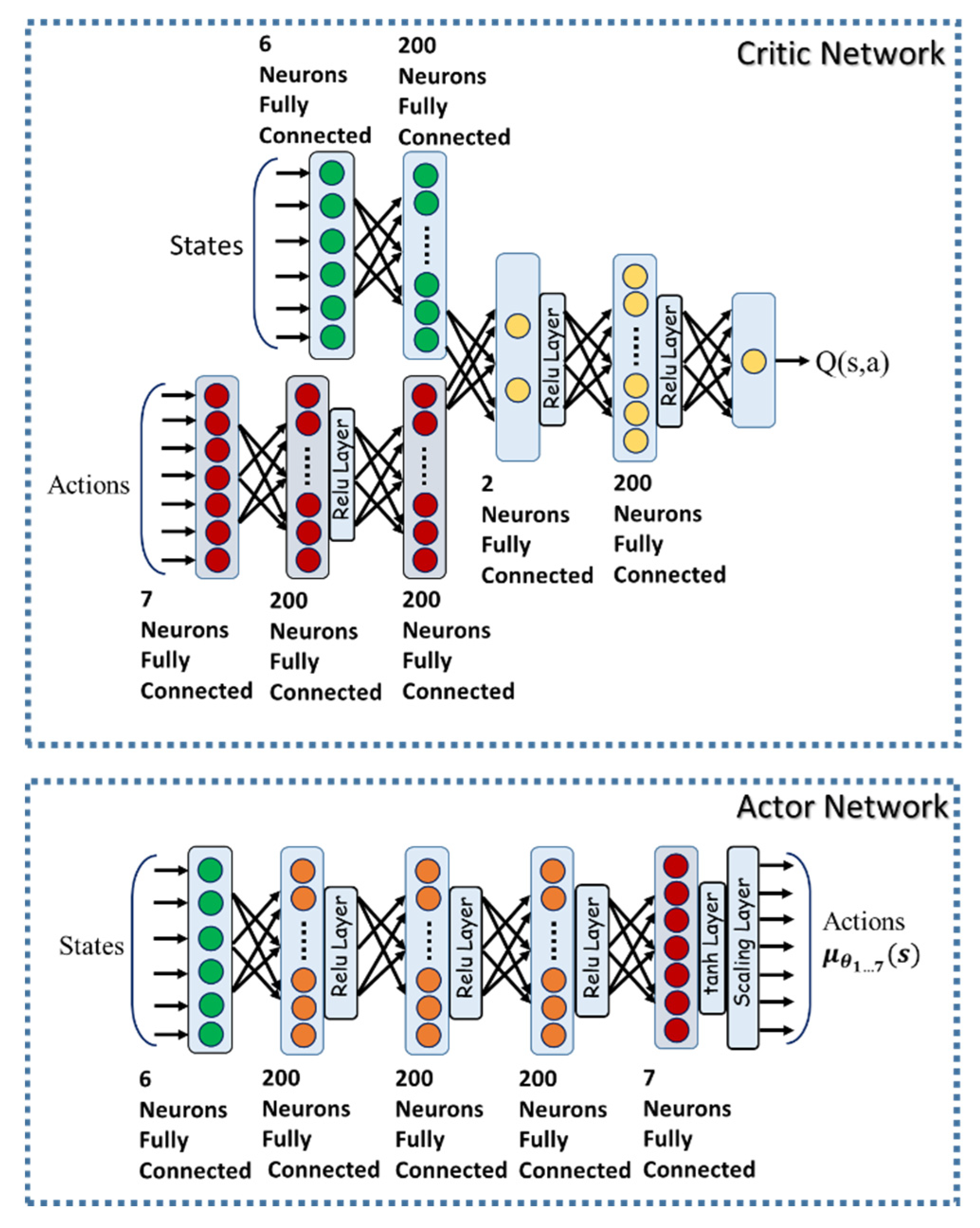
To find the optimal architecture for the actor-critic network, many simulations were run with different numbers of layers and neuron counts in neural networks. According to the simulations findings, it was observed that increasing the size of hidden layers encourages polynomial exploration, whereas increasing the number of layers promotes exponential exploration. The number of layers in the actor network varied from 1 to 5 for the purpose of the experiment. Increasing the size of the actor network layers to a value of more than 400 neurons per layer resulted in over-parameterization and oscillation of the discounted long-term reward. Over-reducing the number of layers, on the other hand, resulted in poor performance. According to the simulation results, it was concluded that at least 130 neurons in each layer of the actor and the critic are necessary to learn the policy effectively, with 200 being the ideal number. The architecture of the designed actor and critic neural networks is shown in Figure 6.
4. Simulations
As mentioned in Section 3, a dynamics model of a commercial aerial robot (Parrot) was selected and implemented in the simulator environment as an aerial robot under control to test the effectiveness of the proposed control architecture in controlling an aerial robot. The AR Drone 2.0, the Rolling Spider, and Mambo are all Parrot products that can be programmed using MATLAB [51]. The AR Drone 2.0 toolbox was developed and distributed by researchers. In addition, a MATLAB Simulink Support Package for Rolling Spider is available as an add-on development package based on MIT’s Aerospace Blockset supporting simulation, hardware code generation, and interface for Parrot Minidrones [52]. The Parrot Mambo (6-DOF small quadcopter) comes with ultrasonic, accelerometer, gyroscope, air pressure, and down-facing camera sensors. It allows algorithms to be applied to the robot via a Bluetooth link over a Personal Area Network (PAN).The Simulink Support Package for Parrot Minidrones [53], which is developed using the UAV toolbox from Mathworks [54], was utilized in this research study to simulate the quadrotor. The aerodynamics effect was deemed minor for the purpose of simplicity, hence the block associated with the aerodynamics effect was deactivated throughout the simulations. Furthermore, during the simulations, parameters of the environment (such as air pressure at various elevations) were also assumed to be constant. A UAV waypoint follower block (included in the UAV toolbox) was employed to generate several successive waypoints. In the Simulink environment, two experiments were carried out to evaluate the performance of the proposed control architecture, compared to that of typical PID controllers.
The experiments aimed at evaluating the effectiveness of the controller in controlling the aerial robot in the presence of weight disturbances affecting the dynamics model of the robot. When a payload is attached to a quadrotor, three main changes may happen. The overall mass of the system increases. The fluctuations in the mass of the robot can also shift the gravitational center, and therefore the inertia. In the experiments, the payload was considered to be an isotropic symmetric stiff solid mass connected to the aerial robot, rather than being suspended. Another assumption was that the physical dimensions of the attached mass were smaller than the dimensions of the quadrotor. The distance between the center of gravity of the robot and the center of gravity of the load is associated with the shape and the weight distribution of the connector, as well as with the shape and the weight distribution of the load. In our experiments, this distance was assumed to be zero. As a result, the effects of changes in inertia and gravity were deemed insignificant. Therefore, the focus of our article was solely on analyzing the effects of mass variation on the performance of the controller. When the robot is executing a logistic task, the mass could be in two stable states: one before the load comes into contact with the quadrotor, and the other when the payload mass is integrated into the system. Depending on the gripping technique and the qualities of the surface of the load, there may be many profiles of mass fluctuation between these two states. We assumed that there was no gripping and the mass was connected to the robot body directly. Another assumption was that the load had a non-deformable surface; therefore, a single step profile for the mass disturbance could be used, as it was implemented in many prior publications. The variations in the mass were simulated by adding a term named to (16)–(18), resulting in Equations (54)–(56). is calculated using Equation (57).
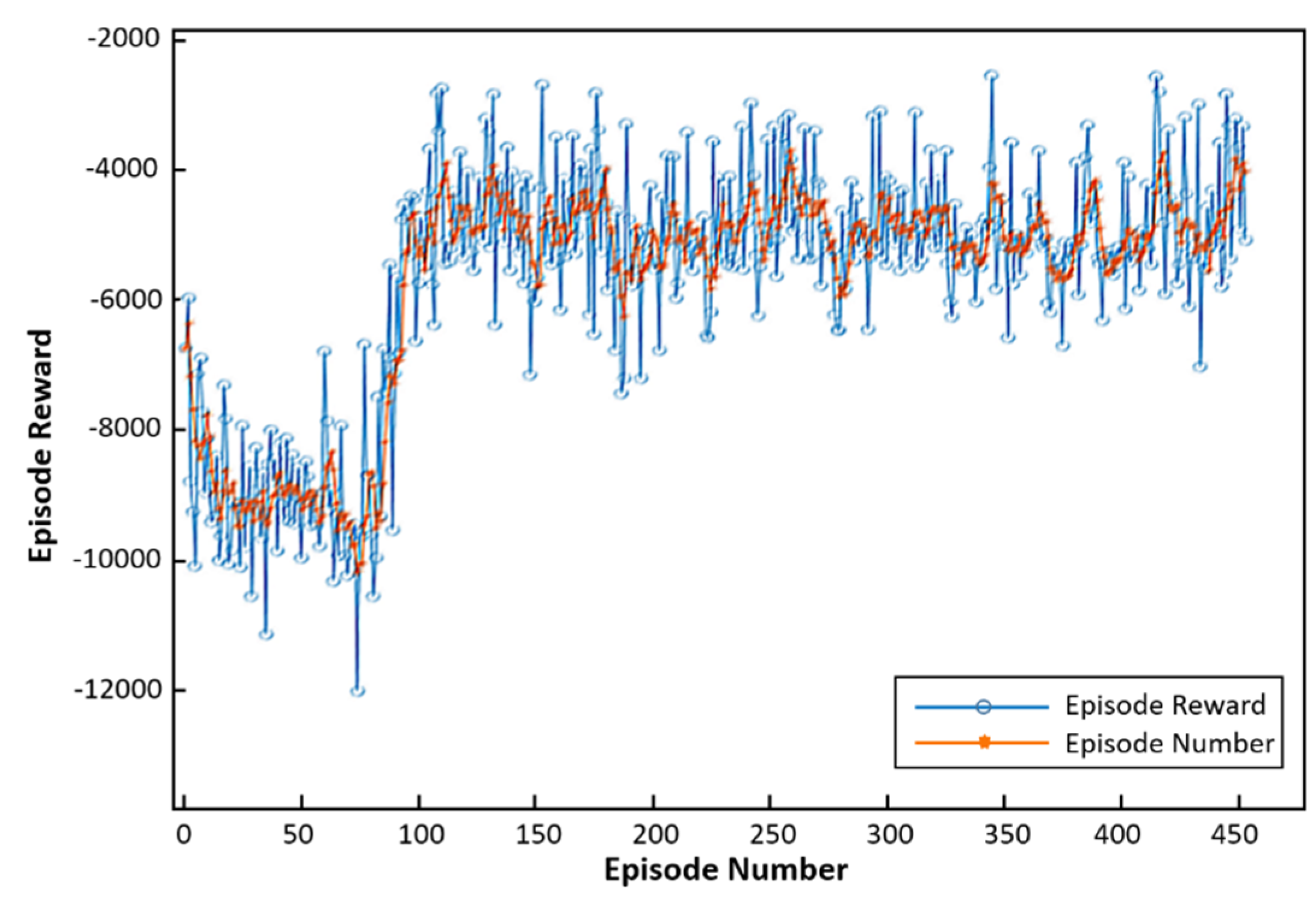
In Equation (57), “Rand” represents a random value between 0% and 70% of the mass of the robot. Every 5 seconds, the mass of the robot is perturbed by a weight disturbance with the value of . An RL agent block from the reinforcement learning toolbox was used in the Simulink environment to implement the deep reinforcement learning policy. During the experiments, the presented RL algorithm interacted with the environment in the simulator, thereby learning the appropriate strategy for estimating and updating the parameters of the PID controllers and the gravity compensator. The achieved reward throughout the training process is shown in Figure 7.
To train the neural networks, different values for hyperparameters were applied, aimed at finding the best possible values. Table 4 shows the optimal values obtained for the hyperparameters.
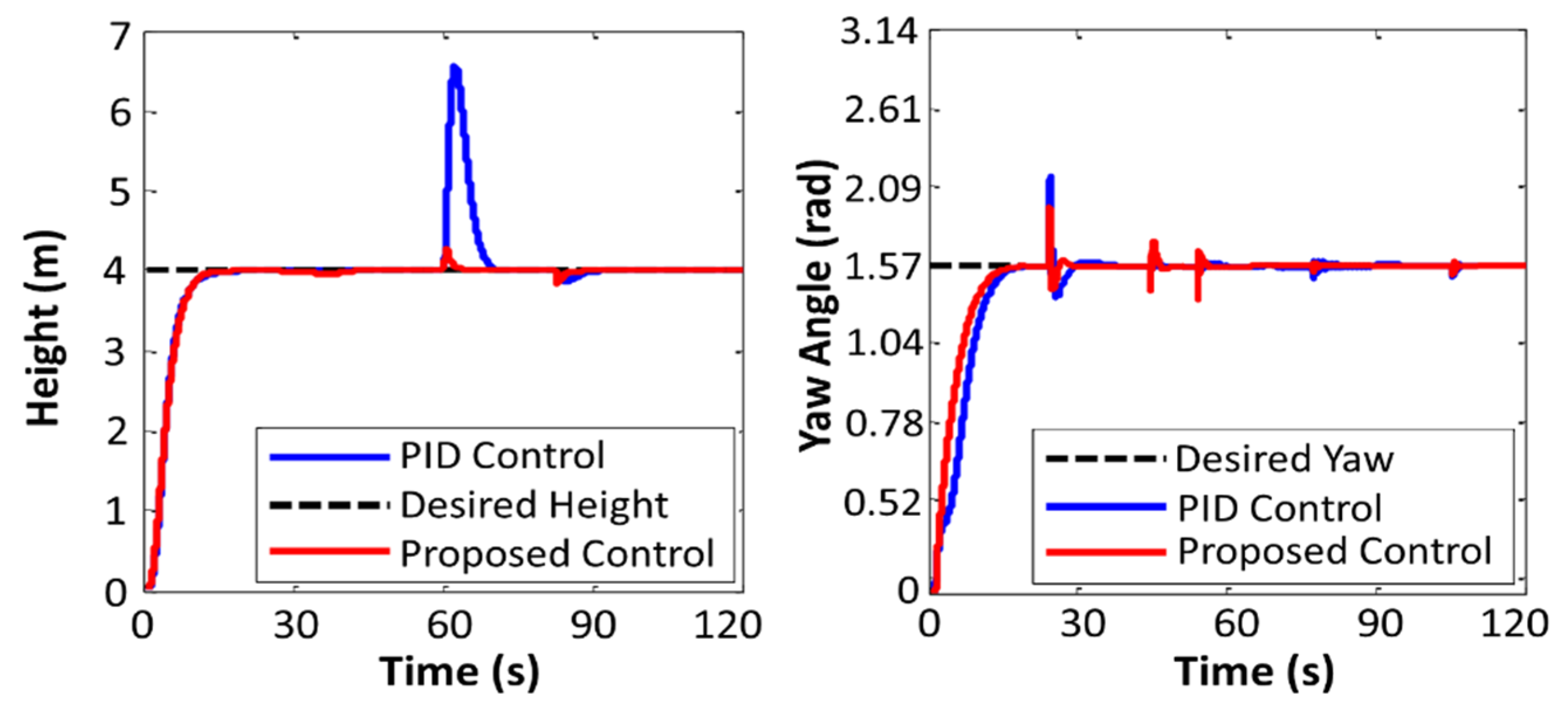
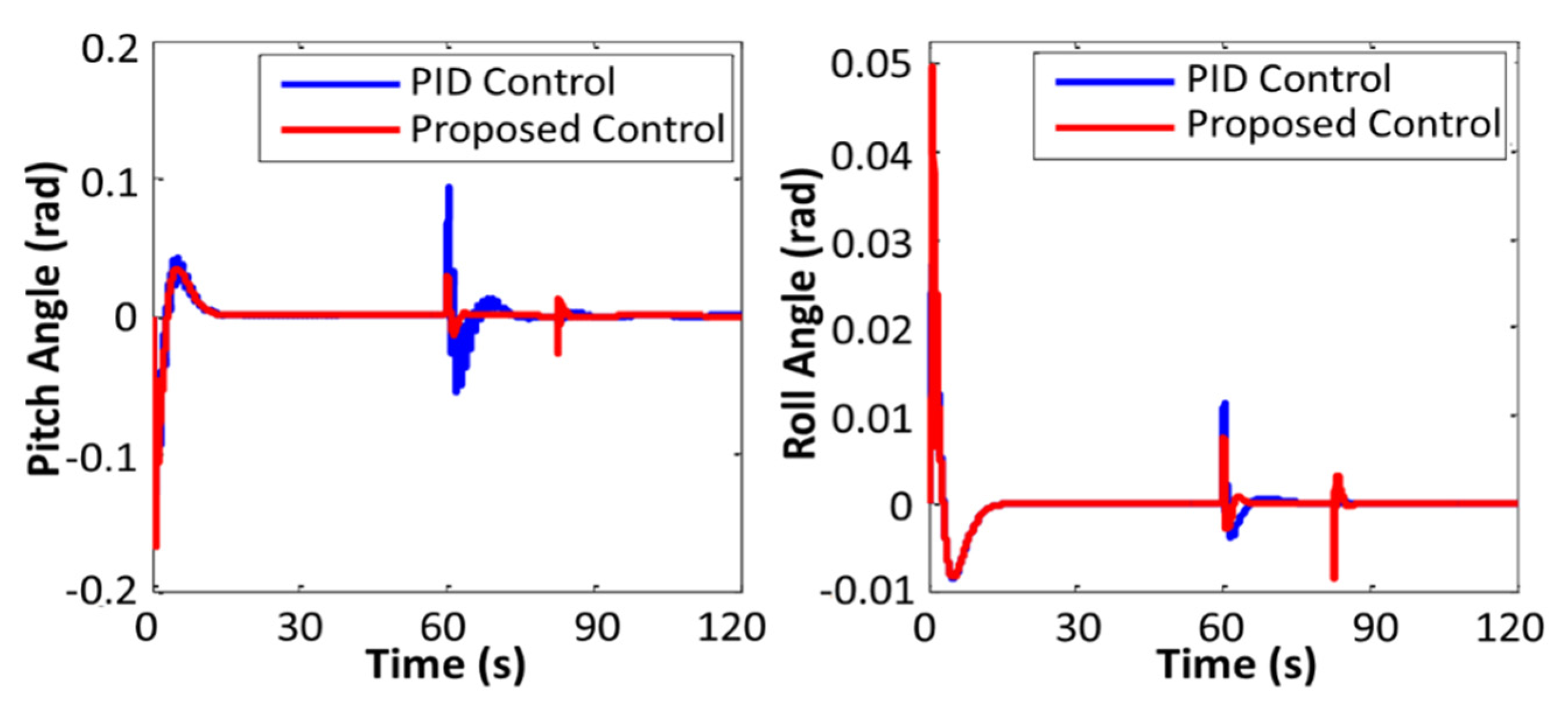
During the aerial robot operation, the trained policy actively estimated the parameters of the controllers. The first experiment was done in two stages (the first time with the proposed controller and the second time with conventional PID controllers) to compare the performance of the proposed controller with that of the conventional PID controller. During the experiments, some weight disturbances (random values between 0% and 70% of the mass of the robot) perturbed the system. The first defined maneuver for the aerial robot was to get to the coordinates (x, y, z = 3.5, 3.5, 4) and stabilize its position in space. Figure 8, Figure 9 and Figure 10 show the performance of the PID controller and the proposed controller.
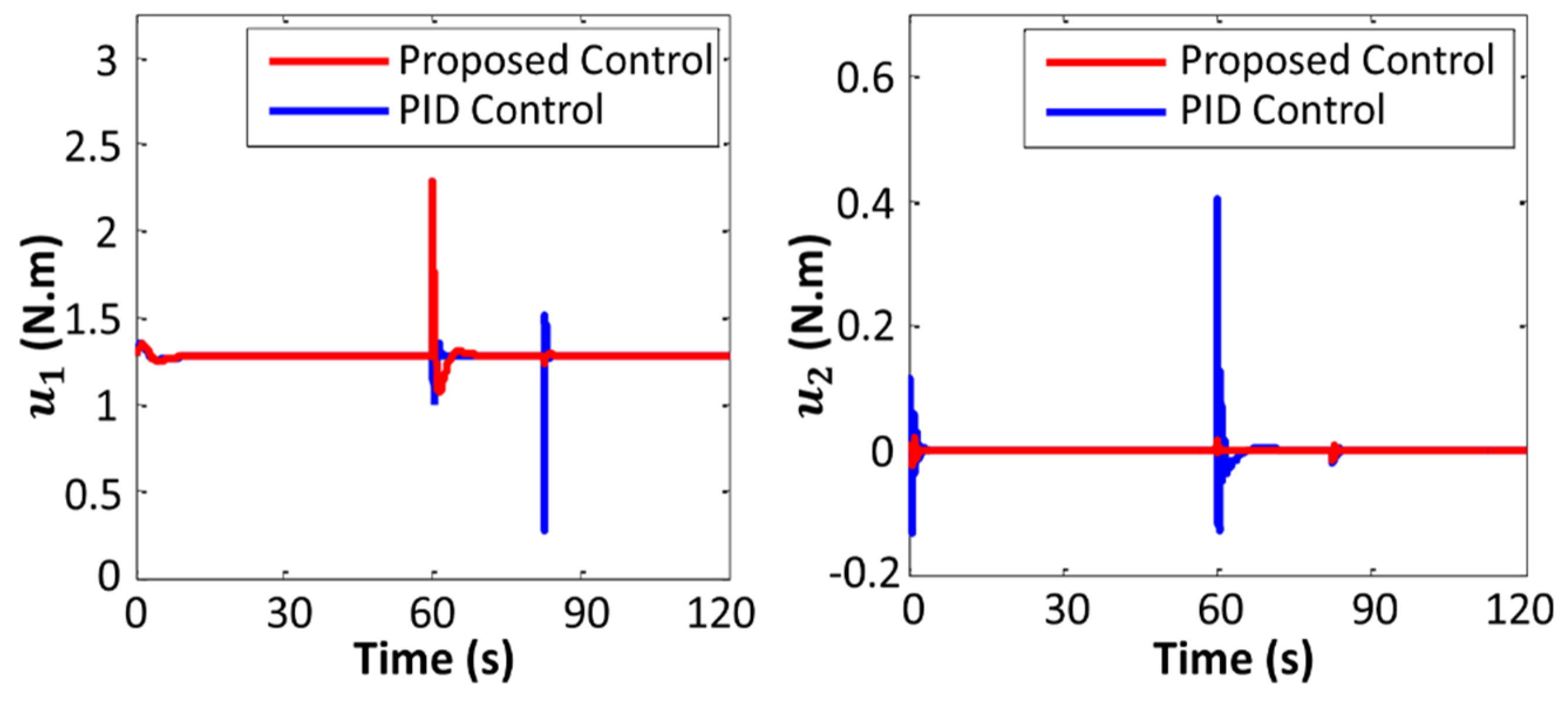
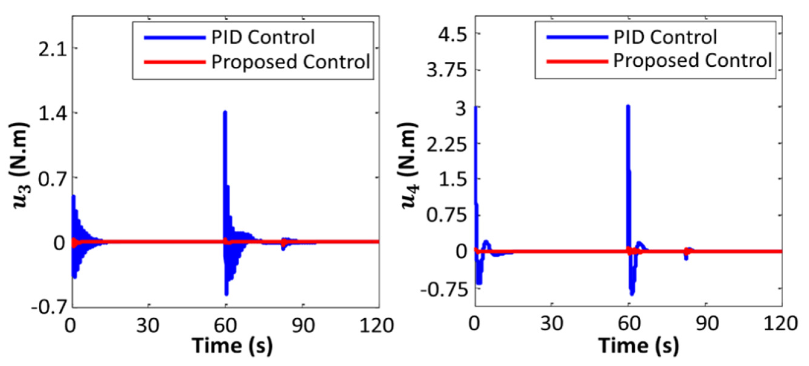
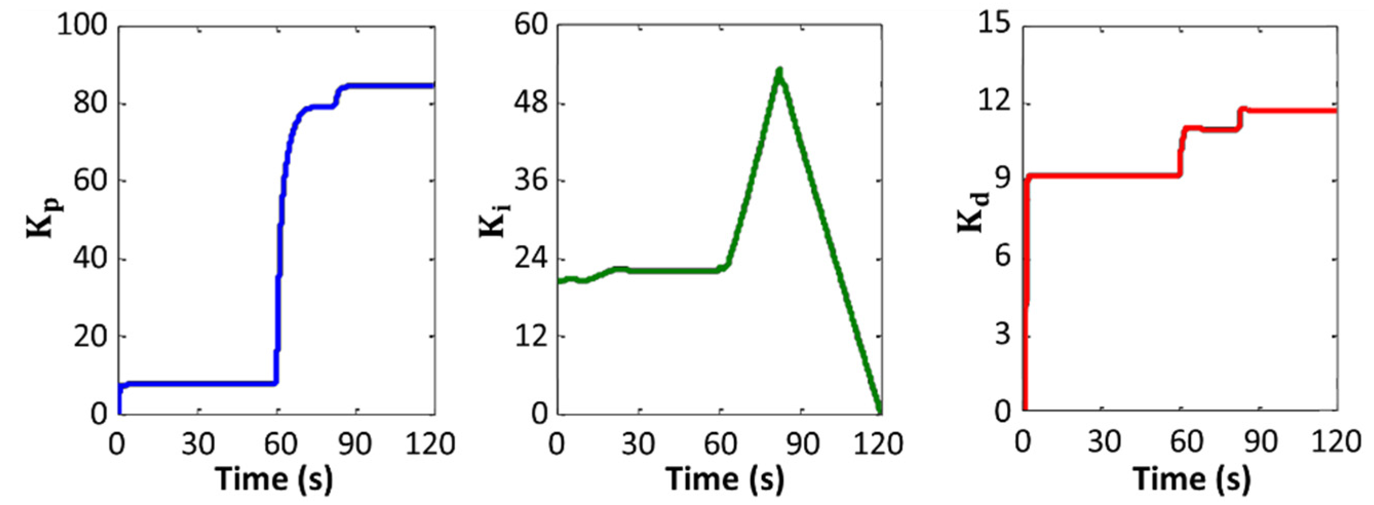
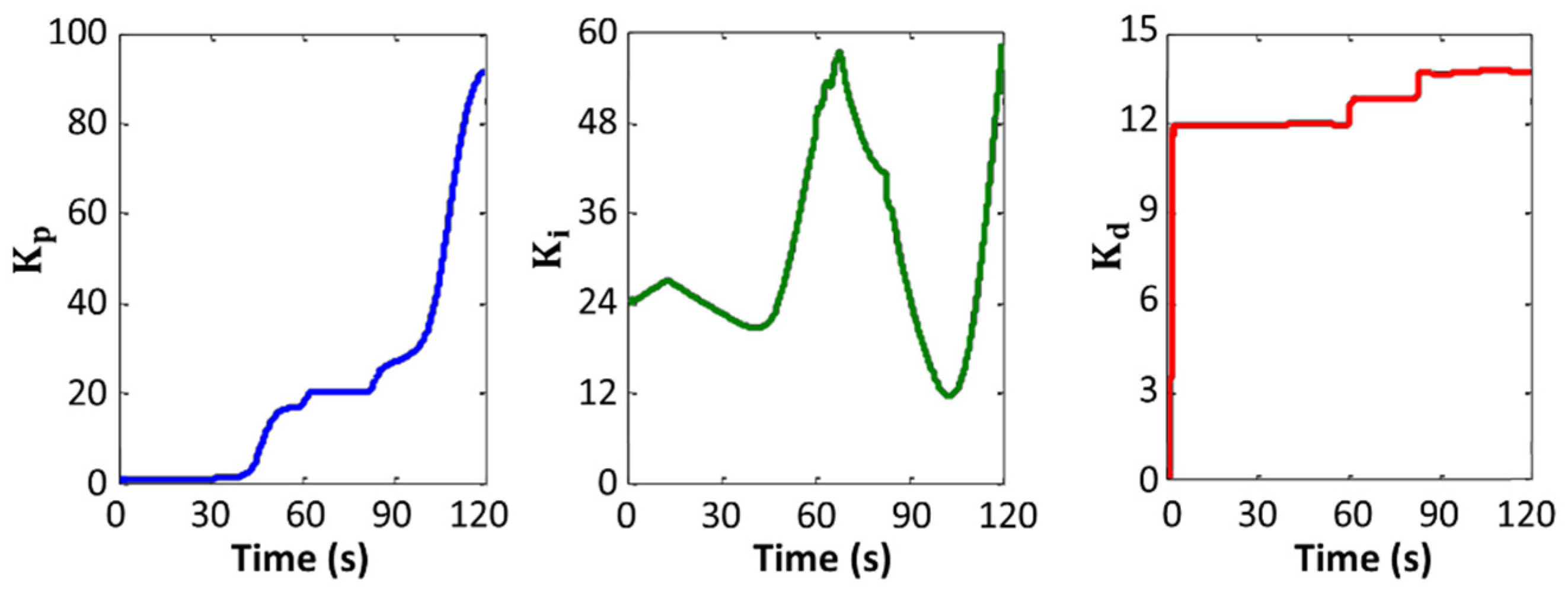
Variations in the values of the manipulated variables are plotted in Figure 11 and Figure 12. Figure 13 and Figure 14 exhibit changes in control gain values that occurred during the operation of the robot.
A comparative study using a range of values was conducted to explore the influence of RL hyperparameters on the steady-state error of the altitude control. According to the results of the experiments, zero noise generated the highest steady-state error. Setting the noise to a very high value, however, prevented the actor from learning the best policy, resulting in more errors. It was observed that increasing the variance enhances the exploration of action space. For both actor and critic, the gradient threshold varied between 1, 4, and infinity. Table 5 summarizes the results of the trials.
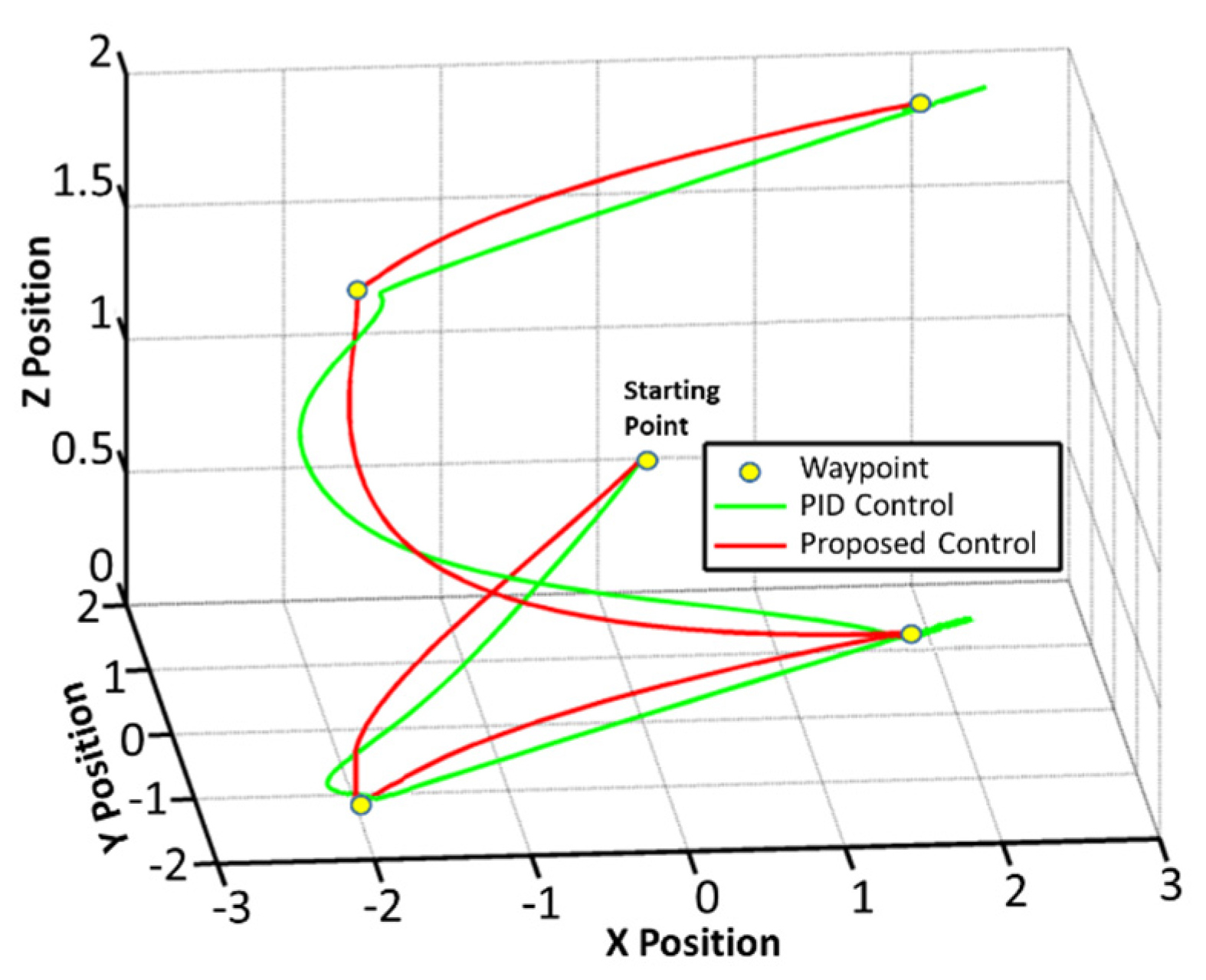
In the second experiment, a waypoint tracking maneuver was conducted to evaluate the ability of the robot, with the proposed control architecture, in tracking consecutive waypoints. Figure 15 illustrates the performance of the aerial robot in tracking the waypoints.
From the results of the experiments, it can be observed that the robot with the proposed controller provided smoother trajectory. Furthermore, the error in the trajectory tracking of the robot with the proposed controller was less than that of the PID controller. The results showed that the proposed control algorithm is able to stabilize the system performance when the robot is subjected to weight disturbances. It must be noted that the performance of the conventional PID controller was satisfactory as long as the extra weight was low, but when the added weight was large, the basic PID controller failed to control the robot properly.
5. Conclusions
A new deep reinforcement learning-based adaptive controller for controlling an aerial robot was proposed in this research paper. To interact with the robot dynamics model and learn the right policy for actively adjusting the controller, the proposed adaptive control method leveraged a deep deterministic policy gradient algorithm. A linear model predictive controller and an adaptive gravity compensator gain were used in the proposed control system for the robot altitude controller. The performance of the proposed control architecture was compared to that of traditional PID controllers with fixed settings in the Simulink environment. Experiments in a simulated environment demonstrated that the presented control algorithm outperforms ordinary PID controllers in terms of trajectory tracking and altitude control.
Author Contributions
Conceptualization, A.B. and D.-J.L.; methodology, A.B.; software, A.B.; validation, A.B.; formal analysis, A.B.; investigation, A.B.; resources, A.B.; writing—original draft preparation, A.B.; writing—review and editing, A.B.; visualization, A.B.; supervision, D.-J.L.; project administration, D.-J.L.; funding acquisition, D.-J.L. All authors have read and agreed to the published version of the manuscript.
Funding
This research was supported by the Unmanned Vehicles Core Technology Research and Development Program through the National Research Foundation of Korea (NRF), Unmanned Vehicle Advanced Research Center (UVARC), which is funded by the Ministry of Science and ICT, the Republic of Korea (2020M3C1C1A01082375). This research was also supported by DNA+Drone Technology Development Program through the National Research Foundation of Korea (NRF), which is funded by the Ministry of Science and ICT (No. NRF-2020M3C1C2A01080819).
Conflicts of Interest
The authors declare no conflict of interest.
References
- Saunders, J.; Saeedi, S.; Li, W. Autonomous Aerial Delivery Vehicles, a Survey of Techniques on how Aerial Package Delivery is Achieved. arXiv 2021, arXiv:2110.02429. [Google Scholar]
- Joshi, G.; Virdi, J.; Chowdhary, G. Design and flight evaluation of deep model reference adaptive controller. In Proceedings of the AIAA Scitech 2020 Forum, Orlando, FL, USA, 6–10 January 2020; p. 1336. [Google Scholar]
- Balcazar, R.; Rubio, J.D.J.; Orozco, E.; Cordova, D.A.; Ochoa, G.; Garcia, E.; Pacheco, J.; Gutierrez, G.J.; Mujica-Vargas, D.; Aguilar-Ibañez, C. The Regulation of an Electric Oven and an Inverted Pendulum. Symmetry 2022, 14, 759. [Google Scholar] [CrossRef]
- Rubio, J.D.J.; Orozco, E.; Cordova, D.A.; Islas, M.A.; Pacheco, J.; Gutierrez, G.J.; Zacarias, A.; Soriano, L.A.; Meda-Campana, J.A.; Mujica-Vargas, D. Modified Linear Technique for the Controllability and Observability of Robotic Arms. IEEE Access 2022, 10, 3366–3377. [Google Scholar] [CrossRef]
- Aguilar-Ibanez, C.; Moreno-Valenzuela, J.; García-Alarcón, O.; Martinez-Lopez, M.; Acosta, J.Á.; Suarez-Castanon, M.S. PI-Type Controllers and Σ–Δ Modulation for Saturated DC-DC Buck Power Converters. IEEE Access 2021, 9, 20346–20357. [Google Scholar] [CrossRef]
- Soriano, L.A.; Rubio, J.D.J.; Orozco, E.; Cordova, D.A.; Ochoa, G.; Balcazar, R.; Cruz, D.R.; Meda-Campaña, J.A.; Zacarias, A.; Gutierrez, G.J. Optimization of Sliding Mode Control to Save Energy in a SCARA Robot. Mathematics 2021, 9, 3160. [Google Scholar] [CrossRef]
- Vosoogh, M.; Piltan, F.; Mirshekaran, A.M.; Barzegar, A.; Siahbazi, A.; Sulaiman, N. Integral Criterion-Based Adaptation Control to Vibration Reduction in Sensitive Actuators. Int. J. Hybrid Inf. Technol. 2015, 8, 11–30. [Google Scholar] [CrossRef]
- Soriano, L.A.; Zamora, E.; Vazquez-Nicolas, J.M.; Hernández, G.; Madrigal, J.A.B.; Balderas, D. PD Control Compensation Based on a Cascade Neural Network Applied to a Robot Manipulator. Front. Neurorobotics 2020, 14, 78. [Google Scholar] [CrossRef]
- Kada, B.; Ghazzawi, Y. Robust PID controller design for an UAV flight control system. In Proceedings of the World Congress on Engineering and Computer Science, San Francisco, CA, USA, 19–21 October 2011; Volume 2, pp. 1–6. [Google Scholar]
- Silva-Ortigoza, R.; Hernández-Márquez, E.; Roldán-Caballero, A.; Tavera-Mosqueda, S.; Marciano-Melchor, M.; García-Sánchez, J.R.; Hernández-Guzmán, V.M.; Silva-Ortigoza, G. Sensorless Tracking Control for a “Full-Bridge Buck Inverter–DC Motor” System: Passivity and Flatness-Based Design. IEEE Access 2021, 9, 132191–132204. [Google Scholar] [CrossRef]
- Mirshekaran, A.M.; Piltan, F.; Sulaiman, N.; Siahbazi, A.; Barzegar, A.; Vosoogh, M. Design Intelligent Model-free Hybrid Guidance Controller for Three Dimension Motor. Int. J. Inf. Eng. Electron. Bus. 2014, 6, 29–35. [Google Scholar] [CrossRef] [Green Version]
- Barzegar, A.; Piltan, F.; Mirshekaran, A.M.; Siahbazi, A.; Vosoogh, M.; Sulaiman, N. Research on Hand Tremors-Free in Active Joint Dental Automation. Int. J. Hybrid Inf. Technol. 2015, 8, 71–96. [Google Scholar] [CrossRef]
- He, X.; Kou, G.; Calaf, M.; Leang, K.K. In-Ground-Effect Modeling and Nonlinear-Disturbance Observer for Multirotor Unmanned Aerial Vehicle Control. J. Dyn. Syst. Meas. Control 2019, 141, 071013. [Google Scholar] [CrossRef] [Green Version]
- Barzegar, A.; Doukhi, O.; Lee, D.J.; Jo, Y.H. Nonlinear Model Predictive Control for Self-Driving cars Tra-jectory Tracking in GNSS-denied environments. In Proceedings of the 2020 20th International Conference on Control, Automation and Systems (ICCAS), Busan, Korea, 13–16 October 2020; IEEE: Piscataway, NJ, USA, 2020; pp. 750–755. [Google Scholar]
- Cao, G.; Lai, E.M.-K.; Alam, F. Gaussian Process Model Predictive Control of an Unmanned Quadrotor. J. Intell. Robot. Syst. 2017, 88, 147–162. [Google Scholar] [CrossRef] [Green Version]
- Mehndiratta, M.; Kayacan, E. Gaussian Process-based Learning Control of Aerial Robots for Precise Visualization of Geological Outcrops. In Proceedings of the 2020 European Control Conference (ECC), St. Petersburg, Russia, 12–15 May 2020; IEEE: Piscataway, NJ, USA, 2020; pp. 10–16. [Google Scholar] [CrossRef]
- Caldwell, J.; Marshall, J.A. Towards Efficient Learning-Based Model Predictive Control via Feedback Lineari-zation and Gaussian Process Regression. In Proceedings of the 2021 IEEE/RSJ International Conference on Intelligent Robots and Systems (IROS), Prague, Czech Republic, 27 September–1 October 2021; IEEE: Piscataway, NJ, USA, 2021; pp. 4306–4311. [Google Scholar]
- Chee, K.Y.; Jiahao, T.Z.; Hsieh, M.A. KNODE-MPC: A Knowledge-Based Data-Driven Predictive Control Framework for Aerial Robots. IEEE Robot. Autom. Lett. 2022, 7, 2819–2826. [Google Scholar] [CrossRef]
- Richards, A.; How, J. Decentralized model predictive control of cooperating UAVs. In Proceedings of the 2004 43rd IEEE Conference on Decision and Control (CDC) (IEEE Cat. No. 04CH37601), Nassau, Bahamas, 14–17 December 2004; IEEE: Piscataway, NJ, USA, 2004; Volume 4, pp. 4286–4291. [Google Scholar]
- Scholte, E.; Campbell, M. Robust Nonlinear Model Predictive Control With Partial State Information. IEEE Trans. Control Syst. Technol. 2008, 16, 636–651. [Google Scholar] [CrossRef]
- Mathisen, S.H.; Gryte, K.; Johansen, T.; Fossen, T.I. Non-linear Model Predictive Control for Longitudinal and Lateral Guidance of a Small Fixed-Wing UAV in Precision Deep Stall Landing. In Proceedings of the AIAA Infotech@ Aerospace, San Diego, CA, USA, 4–8 January 2016; p. 0512. [Google Scholar] [CrossRef] [Green Version]
- Barzegar, A.; Doukhi, O.; Lee, D.-J. Design and Implementation of an Autonomous Electric Vehicle for Self-Driving Control under GNSS-Denied Environments. Appl. Sci. 2021, 11, 3688. [Google Scholar] [CrossRef]
- Iskandarani, M.; Givigi, S.N.; Fusina, G.; Beaulieu, A. Unmanned Aerial Vehicle formation flying using Linear Model Predictive Control. In Proceedings of the 2014 IEEE International Systems Conference Proceedings, Ottawa, ON, Canada, 31 March–3 April 2014; IEEE: Piscataway, NJ, USA, 2014; pp. 18–23. [Google Scholar] [CrossRef]
- Britzelmeier, A.; Gerdts, M. A Nonsmooth Newton Method for Linear Model-Predictive Control in Tracking Tasks for a Mobile Robot with Obstacle Avoidance. IEEE Control Syst. Lett. 2020, 4, 886–891. [Google Scholar] [CrossRef]
- Wang, Q.; Zhang, A.; Sun, H.Y. MPC and SADE for UAV real-time path planning in 3D environment. In Proceedings 2014 IEEE International Conference on Security, Pattern Analysis, and Cybernetics (SPAC), Wuhan, China, 18–19 October 2014; IEEE: Piscataway, NJ, USA, 2014; pp. 130–133. [Google Scholar] [CrossRef]
- Pan, Z.; Li, D.; Yang, K.; Deng, H. Multi-Robot Obstacle Avoidance Based on the Improved Artificial Potential Field and PID Adaptive Tracking Control Algorithm. Robotica 2019, 37, 1883–1903. [Google Scholar] [CrossRef]
- Doukhi, O.; Fayjie, A.R.; Lee, D.J. Intelligent Controller Design for Quad-Rotor Stabilization in Presence of Parameter Variations. J. Adv. Transp. 2017, 2017, 4683912. [Google Scholar] [CrossRef] [Green Version]
- Rosales, C.D.; Tosetti, S.R.; Soria, C.M.; Rossomando, F.G. Neural Adaptive PID Control of a Quadrotor using EFK. IEEE Lat. Am. Trans. 2018, 16, 2722–2730. [Google Scholar] [CrossRef]
- Rosales, C.; Soria, C.M.; Rossomando, F.G. Identification and adaptive PID Control of a hexacopter UAV based on neural networks. Int. J. Adapt. Control Signal Process. 2018, 33, 74–91. [Google Scholar] [CrossRef] [Green Version]
- Sarhan, A.; Qin, S. Adaptive PID Control of UAV Altitude Dynamics Based on Parameter Optimization with Fuzzy Inference. Int. J. Model. Optim. 2016, 6, 246–251. [Google Scholar] [CrossRef] [Green Version]
- Siahbazi, A.; Barzegar, A.; Vosoogh, M.; Mirshekaran, A.M.; Soltani, S. Design Modified Sliding Mode Controller with Parallel Fuzzy Inference System Compensator to Control of Spherical Motor. Int. J. Intell. Syst. Appl. 2014, 6, 12–25. [Google Scholar] [CrossRef] [Green Version]
- Hu, X.; Liu, J. Research on uav balance control based on expert-fuzzy adaptive pid. In Proceedings of the 2020 IEEE International Conference on Advances in Electrical Engineering and Computer Applications (AEECA), Dalian, China, 25–27 August 2020; IEEE: Piscataway, NJ, USA, 2020; pp. 787–789. [Google Scholar]
- Barzegar, A.; Piltan, F.; Vosoogh, M.; Mirshekaran, A.M.; Siahbazi, A. Design Serial Intelligent Modified Feedback Linearization like Controller with Application to Spherical Motor. Int. J. Inf. Technol. Comput. Sci. 2014, 6, 72–83. [Google Scholar] [CrossRef] [Green Version]
- Duan, Y.; Chen, X.; Houthooft, R.; Schulman, J.; Abbeel, P. Benchmarking deep reinforcement learning for continuous control. In Proceedings of the International Conference on Machine Learning, New York, NY, USA, 20–22 June 2016; PMLR: London, UK, 2016; pp. 1329–1338. [Google Scholar]
- Kober, J.; Bagnell, J.A.; Peters, J. Reinforcement learning in robotics: A survey. Int. J. Robot. Res. 2013, 32, 1238–1274. [Google Scholar] [CrossRef] [Green Version]
- Claus, C.; Boutilier, C. The dynamics of reinforcement learning in cooperative multiagent systems. In Proceedings of the Fifteenth National/Tenth Conference on Artificial Intelligence/Innovative Applications of Artificial Intelligence, Madison, WI, USA, 26–30 July 1998; pp. 746–752. [Google Scholar]
- Bernstein, A.V.; Burnaev, E.V. Reinforcement learning in computer vision. In Proceedings of the Tenth International Conference on Machine Vision (ICMV 2017), Vienna, Austria, 13–15 November 2048; Volume 10696, pp. 458–464. [Google Scholar]
- Bohn, E.; Coates, E.M.; Moe, S.; Johansen, T.A. Deep Reinforcement Learning Attitude Control of Fixed-Wing UAVs Using Proximal Policy optimization. In Proceedings of the 2019 International Conference on Unmanned Aircraft Systems (ICUAS), Atlanta, GA, USA, 11–14 June 2019; IEEE: Piscataway, NJ, USA, 2019; pp. 523–533. [Google Scholar] [CrossRef] [Green Version]
- Koch, W.; Mancuso, R.; West, R.; Bestavros, A. Reinforcement Learning for UAV Attitude Control. ACM Trans. Cyber-Phys. Syst. 2019, 3, 1–21. [Google Scholar] [CrossRef] [Green Version]
- Polvara, R.; Patacchiola, M.; Sharma, S.; Wan, J.; Manning, A.; Sutton, R.; Cangelosi, A. Toward End-to-End Control for UAV Autonomous Landing via Deep Reinforcement Learning. In Proceedings of the 2019 International Conference on Unmanned Aircraft Systems (ICUAS), Dallas, TX, USA, 12–15 June 2018; IEEE: Piscataway, NJ, USA, 2018; pp. 115–123. [Google Scholar] [CrossRef]
- Passalis, N.; Tefas, A. Continuous drone control using deep reinforcement learning for frontal view person shooting. Neural Comput. Appl. 2019, 32, 4227–4238. [Google Scholar] [CrossRef]
- Zheng, L.; Zhou, Z.; Sun, P.; Zhang, Z.; Wang, R. A novel control mode of bionic morphing tail based on deep reinforcement learning. arXiv 2020, arXiv:2010.03814. [Google Scholar]
- Botvinick, M.; Ritter, S.; Wang, J.X.; Kurth-Nelson, Z.; Blundell, C.; Hassabis, D. Reinforcement learning, fast and slow. Trends Cogn. Sci. 2019, 23, 408–422. [Google Scholar] [CrossRef] [Green Version]
- Pi, C.-H.; Ye, W.-Y.; Cheng, S. Robust Quadrotor Control through Reinforcement Learning with Disturbance Compensation. Appl. Sci. 2021, 11, 3257. [Google Scholar] [CrossRef]
- Shi, Q.; Lam, H.-K.; Xuan, C.; Chen, M. Adaptive neuro-fuzzy PID controller based on twin delayed deep deterministic policy gradient algorithm. Neurocomputing 2020, 402, 183–194. [Google Scholar] [CrossRef]
- Dooraki, A.R.; Lee, D.-J. An innovative bio-inspired flight controller for quad-rotor drones: Quad-rotor drone learning to fly using reinforcement learning. Robot. Auton. Syst. 2020, 135, 103671. [Google Scholar] [CrossRef]
- Quan, Q. Introduction to Multicopter Design and Control, 1st ed.; Springer Nature: Singapore, 2017; pp. 99–120. [Google Scholar]
- Hernandez, A.; Copot, C.; De Keyser, R.; Vlas, T.; Nascu, I. Identification and path following control of an AR. Drone quadrotor. In Proceedings of the 2013 17th International Conference on System Theory, Control and Computing (ICSTCC), Sinaia, Romania, 11–13 October 2013; IEEE: Piscataway, NJ, USA, 2013; pp. 583–588. [Google Scholar]
- Fan, J.; Wang, Z.; Xie, Y.; Yang, Z. A theoretical analysis of deep Q-learning. In Proceedings of the Learning for Dynamics and Control, Virtual, 7–8 June 2020; PMLR: London, UK, 2020; pp. 486–489. [Google Scholar]
- Jesus, C., Jr.; Bottega, J.A.; Cuadros, M.A.S.L.; Gamarra, D.F.T. Deep deterministic policy gradient for navigation of mobile robots in simulated environments. In Proceedings of the 2019 19th International Conference on Advanced Robotics (ICAR), Belo Horizonte, Brazil, 2–6 December 2019; pp. 362–367. [Google Scholar]
- Sandipan, S.; Wadoo, S. Linear optimal control of a parrot AR drone 2.0. In Proceedings of the 2017 IEEE MIT Undergraduate Research Technology Conference (URTC), Cambridge, MA, USA, 3–5 November 2017; IEEE: Piscataway, NJ, USA, 2017; pp. 1–5. [Google Scholar]
- Glazkov, T.V.; Golubev, A.E. Using Simulink Support Package for Parrot Minidrones in nonlinear control education. AIP Conf. Proc. 2019, 2195, 020007. [Google Scholar] [CrossRef]
- Kaplan, M.R.; Eraslan, A.; Beke, A.; Kumbasar, T. Altitude and Position Control of Parrot Mambo Minidrone with PID and Fuzzy PID Controllers. In Proceedings of the 2019 11th International Conference on Electrical and Electronics Engineering (ELECO), Bursa, Turkey, 28–30 November 2019; IEEE: Piscataway, NJ, USA, 2019; pp. 785–789. [Google Scholar] [CrossRef]
- Gill, J.S.; Velashani, M.S.; Wolf, J.; Kenney, J.; Manesh, M.R.; Kaabouch, N. Simulation Testbeds and Frameworks for UAV Performance Evaluation. In Proceedings of the 2021 IEEE International Conference on Electro Information Technology (EIT), Mt. Pleasant, MI, USA, 14–15 May 2021; IEEE: Piscataway, NJ, USA, 2021; pp. 335–341. [Google Scholar]
Figure 1.
The coordinate frame of the quadcopter.

Figure 2.
The elements of the proposed control architecture of the quadcopter.

Figure 3.
Prediction horizon and predicted control inputs in MPC.

Figure 4.
The architecture and learning process of deep deterministic policy gradient.

Figure 5.
The architecture of the proposed adaptive RL-based controller.

Figure 6.
The architecture of actor and critic neural networks.

Figure 7.
Episode reward and average reward recorded during training.

Figure 8.
Performance of the quadcopter in tracking the desired X and Y positions.

Figure 9.
Performance of the quadcopter in attaining desired height and yaw angle.

Figure 10.
Performance of the quadcopter in tracking the desired Roll and Pitch angles.

Figure 11.
Variations in manipulated variables .

Figure 12.
Variations in manipulated variables .

Figure 13.
Variations in adaptive gain values of the X position PID controller.

Figure 14.
Variations in adaptive gain values of the Y position PID controller.

Figure 15.
Performance of the aerial robot in tracking waypoints.


Table 1.
Control gain values of the inner-loop PID controllers.
| PID Control | |||
|---|---|---|---|
| 0.021 | 0.011 | 0.003 | |
| 0.014 | 0.03 | 0.001 | |
| 0.002 | 0.07 | 0.013 |
Table 2.
The Parrot aerial robot model specifications [48].
Table 2.
The Parrot aerial robot model specifications [48].
| Specification | Parameter | Unit | Value |
|---|---|---|---|
| Drone Mass | m | kg | 0.063 |
| Lateral Moment Arm | l | m | 0.0624 |
| Thrust Coefficient | b | N∙s2 | 0.0107 |
| Drag Coefficient | d | N∙m∙s2 | 0.7826 × 10⁻³ |
| Rolling Moment of Inertia | Ix | Kg∙m2 | 5.82857 × 10⁻⁵ |
| Pitching Moment of Inertia | Iy | Kg∙m2 | 7.16914 × 10⁻⁵ |
| Yawing Moment of Inertia | Iz | Kg∙m2 | 0.0001 |
| Rotor Moment of Inertia | Ir | Kg∙m2 | 0.1021 × 10⁻⁶ |
Table 3.
The parameters of the state space model.
| Parameter | Value |
|---|---|
| A | |
| B | |
| C | |
| D |
Table 4.
The optimal values for hyperparameters.
| Hyperparameter | Value |
|---|---|
| Critic Learning Rate | 0.0001 |
| Actor Learning Rate | 0.00001 |
| Critic Gradient Threshold | 1 |
| Actor Gradient Threshold | 4 |
| Variance | 0.3 |
| Variance Decay Rate | 0.00001 |
| Experience Buffer | 1,000,000 |
| Mini-Batch Size | 64 |
| Target Smooth Factor | 0.001 |
Table 5.
Variation of RL hyperparameters and their effect on the steady-state error.
| Critic Learning Rate | Actor Grad Threshold | Critic Grad Threshold | Variance (Noise) | Mini Batch Size | Steady State Error |
|---|---|---|---|---|---|
| 4 | 1 | 0.3 | 64 | 0.00064 | |
| inf | 1 | 0.3 | 64 | 0.00093 | |
| 1 | 4 | 0.3 | 64 | 0.00011 | |
| 1 | inf | 0.3 | 64 | 0.00008 | |
| 1 | 1 | 0 | 64 | 0.00435 | |
| 1 | 1 | 0.5 | 64 | 0.00010 | |
| 1 | 1 | 0.3 | 128 | 0.00045 | |
| 4 | 1 | 0.3 | 64 | 0.00001 |
Publisher’s Note: MDPI stays neutral with regard to jurisdictional claims in published maps and institutional affiliations. |
© 2022 by the authors. Licensee MDPI, Basel, Switzerland. This article is an open access article distributed under the terms and conditions of the Creative Commons Attribution (CC BY) license (https://creativecommons.org/licenses/by/4.0/).
Share and Cite
MDPI and ACS Style
Barzegar, A.; Lee, D.-J. Deep Reinforcement Learning-Based Adaptive Controller for Trajectory Tracking and Altitude Control of an Aerial Robot. Appl. Sci. 2022, 12, 4764. https://0-doi-org.brum.beds.ac.uk/10.3390/app12094764
AMA Style
Barzegar A, Lee D-J. Deep Reinforcement Learning-Based Adaptive Controller for Trajectory Tracking and Altitude Control of an Aerial Robot. Applied Sciences. 2022; 12(9):4764. https://0-doi-org.brum.beds.ac.uk/10.3390/app12094764
Chicago/Turabian StyleBarzegar, Ali, and Deok-Jin Lee. 2022. "Deep Reinforcement Learning-Based Adaptive Controller for Trajectory Tracking and Altitude Control of an Aerial Robot" Applied Sciences 12, no. 9: 4764. https://0-doi-org.brum.beds.ac.uk/10.3390/app12094764
Note that from the first issue of 2016, this journal uses article numbers instead of page numbers. See further details here.