
Editable Image Generation with Consistent Unsupervised Disentanglement Based on GAN

School of Computer Science and Engineering, Anhui University of Science and Technology, Huainan 232001, China
*
Author to whom correspondence should be addressed.
†
These authors contributed equally to this work.
Appl. Sci. 2022, 12(11), 5382; https://0-doi-org.brum.beds.ac.uk/10.3390/app12115382
Submission received: 28 April 2022
/
Revised: 24 May 2022
/
Accepted: 24 May 2022
/
Published: 26 May 2022
(This article belongs to the Special Issue Computer Vision and Pattern Recognition Based on Deep Learning)
Abstract
:Featured Application
This work will be applied to editable image generation. In the future, controllable 3D models can be generated to reduce the workload of film and television or game workers.
Abstract
Generative adversarial networks (GANs) are often used to generate realistic images, and GANs are effective in fitting high-dimensional probability distributions. However, during training, they often produce model collapse, which is the inability of the generative model to map the input noise to the real data distribution. In this work, we propose a model for disentanglement and mitigating model collapse inspired by the relationship between Hessian and Jacobian matrices. This is a concise framework for producing few modifications to the original model while facilitating the disentanglement. Compared to the pre-improvement generative models, our approach modifies the original model architecture only marginally and does not change the training method. Our method shows consistent resistance to model collapse on some image datasets, while outperforming the pre-improvement method in terms of disentanglement.
1. Introduction
In recent years, many frameworks for representing high-dimensional data in an unsupervised manner have proliferated. Among many deep generative methods, generative adversarial networks (GANs) are among the most prominent methods for synthesizing real images. Generative Adversarial Network (GAN) has many meaningful works in high-resolution graph generation [1,2,3,4,5]. The emergence of GANs has made a huge leap in modeling high-dimensional distributed data, which has attracted great research interest. It consists of two networks: a generator and a discriminator, where the generator tries to map the latent data to the real data distribution. However, these data are often highly diverse. Therefore, the training of datasets often brings various model training collapse, both in terms of reduced model generation quality and generation diversity.
To solve this problem, there are three main options: (1) modifying the model architecture to change different architectures for different situations (e.g., AdaGAN [6], D2GAN [7]); (2) achieving better data mapping for the required generative goals by modifying the loss function (e.g., WGAN [8], LSGAN [9], EBAGN [10]); or (3) modifying the hidden space (DeLiGAN [11]). We focus on the model architecture, and we modify the original learning paradigm. This approach does not require large modifications to the original model, which greatly broadens the ease of use and applicability, and allows faster convergence to an equilibrium point.
Such a modified approach makes the model more entangled in the latent space. To cope with this problem, SeFa [12] disassembled the first fully connected layer of the GAN to disentanglement, and it is this layer of disentanglement that makes the overall disentanglement capability very limited. The Hessian GAN [13] minimizes the non-diagonal terms of the Hessian matrix to better learn disentanglement, and this method treats each output independently but lacks holistic constraint, so it lacks competitiveness in spatial representation. To solve this problem, Jacobian (OroJaR) [14] computes the Jacobian matrix of outputs to represent the changes caused by potential inputs, constraining the Jacobian vectors of each dimension to be orthogonal, so it can make it possible to compensate for this problem. Still, this method lacks the hessian penalty for effective access to the second-order of the original model information and weakens the output diversity. We demonstrate the intrinsic connection between these two methods and propose a new method that allows the model to have a clear separation boundary and effective spatial separation.
The mode collapse of the generative adversarial network has existed since the model was produced. Some scholars’ works [15,16,17,18] make the model better to avoid this problem. For using these methods [15,16,17,18], the original model needs to be significantly changed, so we propose our method to mitigate mode collapse.
The method we propose to mitigate mode collapse is dedicated to further reducing the probability of mode collapse based on the original model, which we mainly show through loss line graphs and evaluation metrics. Moreover, our model can mitigate mode collapse without increasing the training burden.
Alleviating model collapse is only the first step in practical training. To generate higher-quality and controllable images, disentanglement is necessary. Some scholars’ works [19,20,21,22,23] have done many works, but they do not perform well in disentanglement with multiple objects and complex scenes, so we propose our disentanglement method. Our method outperforms previous disentanglement performances for multiple objects and complex scenes.
In summary, we propose a new training framework that improves model stability and disentanglement with brief modifications to the model. Our approach allows training the model without getting into a local Nash equilibrium problem and doing the model as a disentanglement process. Our approach encourages discriminators and generators to diversify the generated samples to step out of the local optimum. At the same time, the loss term can make the boundaries of the diverse samples clearer to achieve the diversity of real data. In this framework that we proposed, we can choose to change the model architecture to resist model collapse, or we can choose to add our loss function to solve the entanglement. We conducted some experiments on various GAN models to evaluate the performance of our approach under different datasets. Our method consistently outperforms the pre-improvement learning paradigm in model collapse mitigation and generation quality. In short, this paper makes the following contributions:
- We analyze the intrinsic connections and differences between Hessian regularization and Jacobian regularization.
- We propose a joint Hessian–Jacobian regularization model that enables GAN to encourage models to better disentanglement, while modifying the network architecture using only the hyperparameters in it can also better mitigate model collapse.
- We have done relevant experiments to show that our approach is useful in both mitigating model collapse and disentanglement representations.
2. Related Work
In deep learning, the two main types of unsupervised disentanglement learning are adversarial generative network (GAN) [24] and variational autoencoder (VAE) [25]. Before this, reconstruction networks already existed [26,27], and the creation of GANs brought at the same time the related optimization and disentanglement problems. Among the responses, there are changes in different architectures to modify the model architecture (AdaGAN [6], D2GAN [7]), and by modifying the loss function to achieve better data mapping for the required generative target (WGAN [8], LSGAN [9], EBAGN [10]), and by modifying the hidden space (DeLiGAN [11]).
2.1. Better Model Structure
2.1.1. Modifying the Model Architecture
In the training of the datasets, not all their data streams are connected. So, there are cases where a single generator has difficulty capturing all the streams. Some researchers have turned their attention to the network architecture of GAN. The main focus here is to modify the number of generators or discriminators. AdaGAN [6] improves model performance by aggregating many potential individual predictors to form a composite predictor, but its multiple models and complex training process make training more expensive. BEGAN [28] uses a self-encoder as a classifier and matches the loss distribution of the self-encoder through the loss based on Wasserstein distance. In order to make 3D controllable, Henzler et al. [29] used differentiable rendering learning to represent voxels, and the voxels based on this method were not clear enough to cause artifacts. Heusel et al. [30] proposed two time-scale update rules. Still, this approach tends to make the training of GANs network hard. Even if the regularization term is added, the effect is not very obvious, and the training cost is also high. CGAN [31] is different from GAN, it adds the same condition to both the Generator and the Discriminator and uses this condition to determine the direction of the Generation model. CGAN [31] uses the conditional probability Generation model to generate multiple outputs simultaneously through different inputs of dependent variables. D2GAN [7] uses two discriminators to minimize KL divergence (Kullback–Leibler divergence: KL divergence is used to express the degree of difference between two distributions) and invert KL divergence, and it can solve the model collapse problem to some extent. However, like other methods, D2GAN [7] has the common problem of the computational complexity.
2.1.2. Alternative Loss Functions
InfoGAN [32] proposed an information-theoretic extension of GANs that obtains a deconvoluted representation of the data by penalized latent reconstructions. Mao et al. [9] proposed LSGAN, which uses a least-squares loss function instead of the GAN loss function, and they defined a pullback operator to map the generated samples to the data stream shape, which alleviates the instability of GAN training and poor quality of the generated images. EBGAN [10] provides an energy-based explanation for GAN, and thus can use a series of energy-based tools for GAN. The exhaustive grid search experiment verifies the complete set of hyperparameters and architecture settings of GAN and EBGAN [10]. Radford et al. [33] alleviates the stability of GAN-generated images to some extent, but the generated images lack global uniformity. Arjovsky et al. [8] used Wasserstein distance instead of JS scatter while completing stable training, which is difficult to train and slow to converge during practical experiments. Then, Gulrajani et al. [34] improved WGAN [8] and proposed WGAN-GP, which used weight clipping in dealing with Lipschitz constraints. The method 3D Controllable Image Synthesis proposed by Liao et al. [35] requires pure background images as an auxiliary to process multi-object scenes, which brings differentiable rendering to a new level, and the difficulty of obtaining pure background images reduces to a certain extent the breadth of application of this method. Hessian Penalty [13] achieved orthogonalization by constraining the output to be diagonal to the input Hessian matrix. After that, OroJaR [14] constrained the input by Jacobian matrix dimensions to disentangle the model. BGAN [36] means Boundary Seeking GAN, and it is dedicated to finding the boundary of GAN; this refers to the boundary when the discriminator’s loss is generally stable at 0.5 because the effect of generating pictures at this time is the best. To obtain the optimal D, Hjelm et al. [36] made some modifications to the loss function. When = 0.5, G is optimal. The opposite approach has been used by [37], in order to make localization operations easier and more meaningful in each semantic region, they used a large number of localization controls by semantic mappings and sorted them, thus achieving the desired effect.
2.2. Disentanglement
Among the existing unsupervised methodological approaches, the two main types of disentanglement representations for GAN are disentanglement in the GAN potential space and regularized disentanglement. GANSPACE [38] applies PCA to the sampled data to find significant and meaningful directions in the style space of StyleGAN [1]. Mildenhall et al. [39] proposed a neural radiation field that combines implicit neural models with volume rendering to reconstruct complex scenes. FineGAN [40] uses information theory with weaker supervised information for background, object pose, shape, and texture to find meaningful orientations. An unsupervised method such as [41] enables the classifier to correctly identify the semantic orientations in the matrix. InfoGAN [32] includes autoencoders on the potential space; however, it has been shown to have similar stability issues to standard GAN and requires stabilization of empirical skills. Giraffe [42] advocates generation directly in the 3D modeling process, and they introduce regularization in 3D modeling. Giraffe [42] can better disentangle a single object, but the disentanglement does not perform well in the multi-object case.
In generation tests, generators still suffer from uneven generation distributions, including collapsed generation content and incomplete semantics. However, these works provide a variety of approaches and solutions that alleviate the generator crash problem to some extent, but the disentanglement does not perform well. Among many existing generative frameworks, GANs tend to synthesize the highest quality generation. However, they are more difficult to optimize due to unstable training dynamics. Compared to previous methods, our approach requires neither too much change in the model structure nor any additional trainable parameters to achieve a better Nash equilibrium and less overfitting, and a better disentanglement representation.
3. Theoretical Method and Simplified Calculation
In this section, we first introduce the basic theory of GAN dynamics description. Then, we describe the intrinsic unity of the proposed Hessian regularization and Jacobian regularization for learning the disentanglement representation. Finally, we discuss it with related methods (Jacobian (OroJaR) [14] and Hessian penalty [13]) and present our approach.
3.1. Basic Theory and Dynamics of GAN
Generative adversarial networks (GANs) fit the data distribution of generators to the original dataset using a game in which generative models compete with discriminators. The generator G takes a random noise vector as input and maps it to points in the target data distribution. The discriminator D receives the data and tries to determine whether it really comes from the empirical distribution (if so, it outputs 1) or is made by the generator (output 0). During the training iterations, noise vectors from the Gaussian distribution G are pushed through the generator network to form a batch of generated data samples. This process is expressed in the max-min formula as Equation (1)
In Equation (1), denotes the objective function, u denotes the parameters of the generator and v denotes the parameters of the discriminator. In the rest of this paper, G denotes the generator, and D denotes the discriminator. In GAN, x refers to the samples in the real distribution being learned, and z is the target distribution. We set the optimization goal of G to maximize and the optimization goal of D to maximize . In this way, in GAN, we can represent the process as a dynamical system using the ordinary differential equation, and the parameters of this dynamical system consist of two parts: , then Equation (1) combined with the basic equation of GAN can be written as:
In Equation (2), x denotes the training samples and z denotes the noise vectors. GAN is not searching for a globally optimal solution but a local optimal solution. We want the trajectory of the dynamical system to enter a local convergence point, i.e., Nash equilibrium, with continuous iterations, and define the Nash equilibrium point as: , It is easy to prove that for a zero-sum game (f = ), at the Nash equilibrium point, its Jacobian matrix (Equation (3)) is negative definite.
We can determine whether local convergence is reached by checking the properties of the Jacobian matrix. If at some point, its first-order derivative is 0 (as Equation (4)) and its Jacobian matrix is negative definite, then that point is a Nash equilibrium point.
We know that the eigenvalues of semi-negative definite matrices are all less than or equal to zero. Then: if the eigenvalues of the Jacobian matrix at a point are all negative real numbers, the training process converges with a sufficiently small learning rate; if the eigenvalues appear to be complex, the training does not achieve local convergence in general; if the real part of the complex eigenvalues is small and the imaginary part is relatively large, some very demanding learning rate is needed to reach convergence. To deal with this situation, we first analyzed the connection and difference between using the Hessian penalty and the Jacobian discriminant (Section 3.2) and approached this convergence with the Hessian–Jacobian consistent orthogonal method, which is partially seen in Section 3.3.
3.2. Hessian Penalty and Jacobian Penalty
The Hessian penalty and the Jacobian penalty each have their own focus in characterizing the original data distribution. This section focuses on the parts of these two things that we use.
3.2.1. Hessian Penalty
Now consider the Hessian matrix, first making the non-diagonal of the Hessian matrix zero, so that its partial derivatives only act independently in each direction, as Equation (5).
The purpose of this is that has no effect on how the perturbation changes the output of G. The Hessian matrix thus corresponds to the loss , but this is difficult to solve directly for the calculation, and we need to manipulate it further. After estimating it with unbiased empirical variance, we have Equation (6).
where v is the Rademacher vector (each entry has the same −1 or +1) and is the second-order directional derivative of G in the direction v times . Equation (6) can be estimated using the unbiased empirical variance. In practice, we sample a small number of v vectors (usually only two) to compute this empirical variance. The minimizing Equation (6) is equivalent to minimizing the sum of squares of the non-diagonal elements of the Hessian matrix. We quickly calculate the second-order directional derivative term in Equation (7) by the second-order central finite difference approximation.
where > 0 is a hyperparameter that controls the granularity of the second directional derivative estimate. In our implementation, we use = 0.1. Such a Hessian matrix is a square matrix composed of second-order partial derivatives of real-valued functions whose independent variables are vectors. This matrix focuses more on the information change rate of the inverse in the calculation, which corresponds to the extraction and fitting of the surface information (compared to the Jacobi matrix). The Jacobian matrix is a matrix in which the first-order partial derivatives are arranged in a certain way to obtain the Hessian matrix in the shallow features. The Jacobian Penalty corresponding to the Jacobian matrix is described in Section 3.2.2.
3.2.2. Jacobian Penalty
Focusing on the Jacobian matrix, and to more clearly reflect the role of the input parameters and the implied variables on the model, the previous equation in Equation (3) is now replaced by . It is well known that in such a deep generative model, if the correlation coefficients of changes due to different latent dimensions are zero, i.e., , then it is considered that each potential dimension controls the variation of only one variation factor. Using the Jacobian matrix mentioned in the kinetic Equation (4), combined with [14], using the Jacobian vector and constraining it to be orthogonal in different dimensions, we can obtain Equation (8).
In Equation (8), and represents the parameters of the function in different directions in the Z space. Then the G loss of Jacobian penalty becomes the sum of the squared term of Equation (8), and to reduce the computational effort following [43], we rewrite the formula using the Hutchinson estimate as Equation (9).
In Equation (9),we use to represent a Jacobian vector. v is the Rademacher vector (each entry has an equal probability of −1 or 1) and denotes the variance. is the first-order directional derivative in the v times direction. can be efficiently computed by the first-order finite difference approximation as Equation (10).
The operation of this step (Equation (10)) is very similar to the simplification of the Hessian matrix ((Equation (7)), which allows our subsequent calculations to be simplified with similar operations, and it is easy to associate them with each other and the characteristics of their application on GAN networks. We will explain this in Section 3.3.
3.3. Association between the Hessian Penalty and the Jacobian Penalty
In Section 3.2, we have derived through formulas and calculations the Jacobian penalty (Equation (9)) and the Hessian penalty (Equation (6)). Although they target first-order and second-order information on the solution domain, respectively, they are surprisingly consistent in the solution process, which makes practical calculations convenient. We have also analyzed the association between the two for this case. We give our loss at the end of this subsection.
The relationship between the Hessian matrix and the Jacobian matrix is first given: the Hessian matrix is the inverse of the Jacobian matrix of the function’s gradient. The formula expression is in Equation (11).
In Equation (11), f is a function from that transforms points into column vectors. p is is the matrix parameters, denotes the hessian matrix, and denotes the Jacobi after the gradient of the matrix f. Thus, the relationship between the Hessian matrix and the Jacobian matrix can be abbreviated as , considering the nature of matrix operations, so that transposition of the matrix is required in the actual computation.
The Hessian penalty encourages the generator to use the diagonal Hessian of the output concerning the input, using the orthogonalized features as the target of the model, approximated by an unbiased stochastic approximator. The Hessian penalty [13] uses a second-order central finite difference approximation. In contrast, a similar approximation method appears in the same [14], where the Jacobian penalty focuses more on the matrix composed of Jacobian vectors. The orthogonalized features are used as the model’s objective to obtain the corresponding Jacobian objective function. This Jacobi approximation calculation used by [14] differs little from the Hessian penalty.
Approximate Computational Procedure and Loss Function
Considering the Taylor expansion of , we note that the Hessian matrix appears in the local gradient expansion, and we add the Hessian as a linear operator to the expansion to obtain Equation (12)
where is the gradient of , is the incremental value about , and the tail term is the second-order infinitesimal term about . To simplify the calculation, we vectorize , so that , substituting into the equation , we have Equation (13).
In Equation (13), is the scalar and v is the vector, and dividing both sides of Equation (13) by , we have , and removing the infinitesimal term in Equation (13), the formula is equal to Equation (14).
The approximation of the removal of the term() usually brings numerical instability, we need to make small enough, and the effect of can be ignored in actual calculations, is very small, so in the actual calculation, we remove this. The effect of Equation (14) and the calculation procedure is the same as that of the original one.
In order to apply the present method to GAN training, we only need to modify the loss of G as Equation (15). Referring to the derivation of Equation (6) for and Equation (9) for , combined with GAN’s original , we can obtain Equation (15). Here, the values of and are calculated using game theory. For the specific solution process, refer to Appendix A.1. Likewise, the two parameters of this part are also used in the network architecture; for the network architecture algorithm pseudo-code, refer to Appendix A.2.
In Equation (15), and are hyperparameters. The inclusion of and in GAN training is beneficial to learn the representation and to achieve the generation of controllable images. The specific calculations for the hyperparameters and are shown in Appendix A.1. We found that using these hyperparameters only to adjust the training parameters in the model architecture, without using this disentanglement loss in Equation (15), can mitigate the pattern collapse. The use of the hyperparameters in the model is referenced in Appendix A.2.
3.4. Network Model Structure
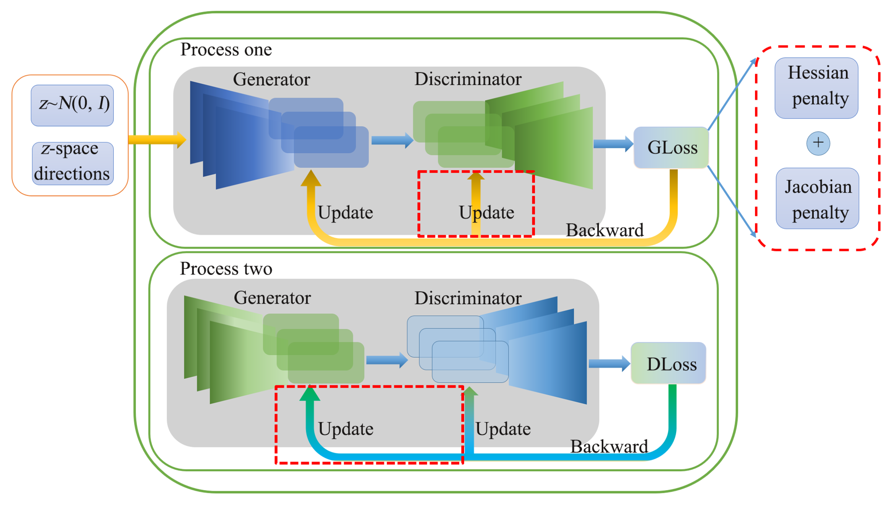
Figure 1 shows the network model proposed in this paper, where the green solid line frame is the original model architecture, and the red dotted lines are the parts added by our method. The green part divides the generative adversarial network training into two processes. The first process updates the generation loss, and the second process updates the discriminant loss. GLoss and DLoss correspond to the loss functions of the generator and discriminator, respectively. Our method is divided into two parts to be added to the model; one is the Update red dashed box in process one and process two, which is mainly used to mitigate mode collapse; the other is the red dashed box corresponding to Gloss. We use Hessian combined with Jacobian for disentangled representation. The two added parts of our model are independent of each other. The red dashed part in the green box is used alone for mode collapse mitigation, and the red dashed part out of the green box is used alone for disentanglement representation.
3.5. Evaluation Metrics
Inception Score (IS) [44] uses an image class classifier to evaluate the quality of the generated images. The image class classifier used is Inception Net-V3. IS is a measure of the clarity and diversity of the generated images, and the bigger the IS value, the better. The specific formula is as Equation (16).
In Equation (16), denotes KL divergence (Kullback–Leibler divergence). For a picture x, the probability distribution that belongs to all classes is . denotes marginal probability.
Fréchet Inception Distance (FID) [30] does not rely on a classifier, but directly considers the distance between the generated data and the real data at the feature level. FID uses the 2048-dimensional vector before the full connection of Inception Net-V3 as the feature of the picture. FID is the distance between the generated image and the real image; the smaller the FID value, the better. The specific formula is as Equation (17).
In Equation (17), denotes the feature mean of the real images. denotes the feature means of the generated images. denotes the covariance matrix of the real images. denotes the covariance matrix of the generated images. Tr denotes the trace of the matrix.
Perceptual Path Length (PPL) [1] subdivides the interpolation path of two noise points into multiple segments, finds the length of each segment, and then averages it. PPL evaluates the distance at which the generator changes from one image to another. The smaller the PPL value, the better.The specific formula is as Equation (18).
In Equation (18), denotes subdivision, replaced with . d denotes perceptual distance, measured using pre-trained VGG. G denotes the image generator. Function slerp denotes spherical linear interpolation, an interpolation method. t denotes the interpolation parameters, subject to the uniform distribution.
4. Experiments
We conducted experiments on datasets such as MNIST, Cifar-10, and ClEVR with several different generative adversarial network models. We evaluate generation based on two criteria: model collapse and generated sample quality. Model collapse and generated sample quality are the two criteria we target and evaluate by Fréchet Inception Distance (FID) [30] and Inception Score (IS) [44]. An important metric for assessing model performance is IS. Calculating IS requires Inception Net-V3 (the third version of Inception Net), and the FID calculates the real samples and generates the distance between samples in the feature space. Different from IS, a lower FID implies higher image quality and diversity.
A comparative test of GANs and the original method is performed to give experimental curves and correlation analysis. Experiments with and were selected, and then our experiments were repeated on other GANs with quantitative analysis. The same architecture and hyperparameters for each method separately ensure fairness in the experiments.
In the disentanglement part, we set all the image sizes to 128 × 128 according to the training arrangement in Hessian. The tested datasets are Edge + Shoes and CLEVR datasets, respectively.
In Section 4.1, we introduce the datasets used for the experiments, and in Section 4.2 and Section 4.3, we test our approach in model collapse and disentanglement.
4.1. Introduction to the Datasets
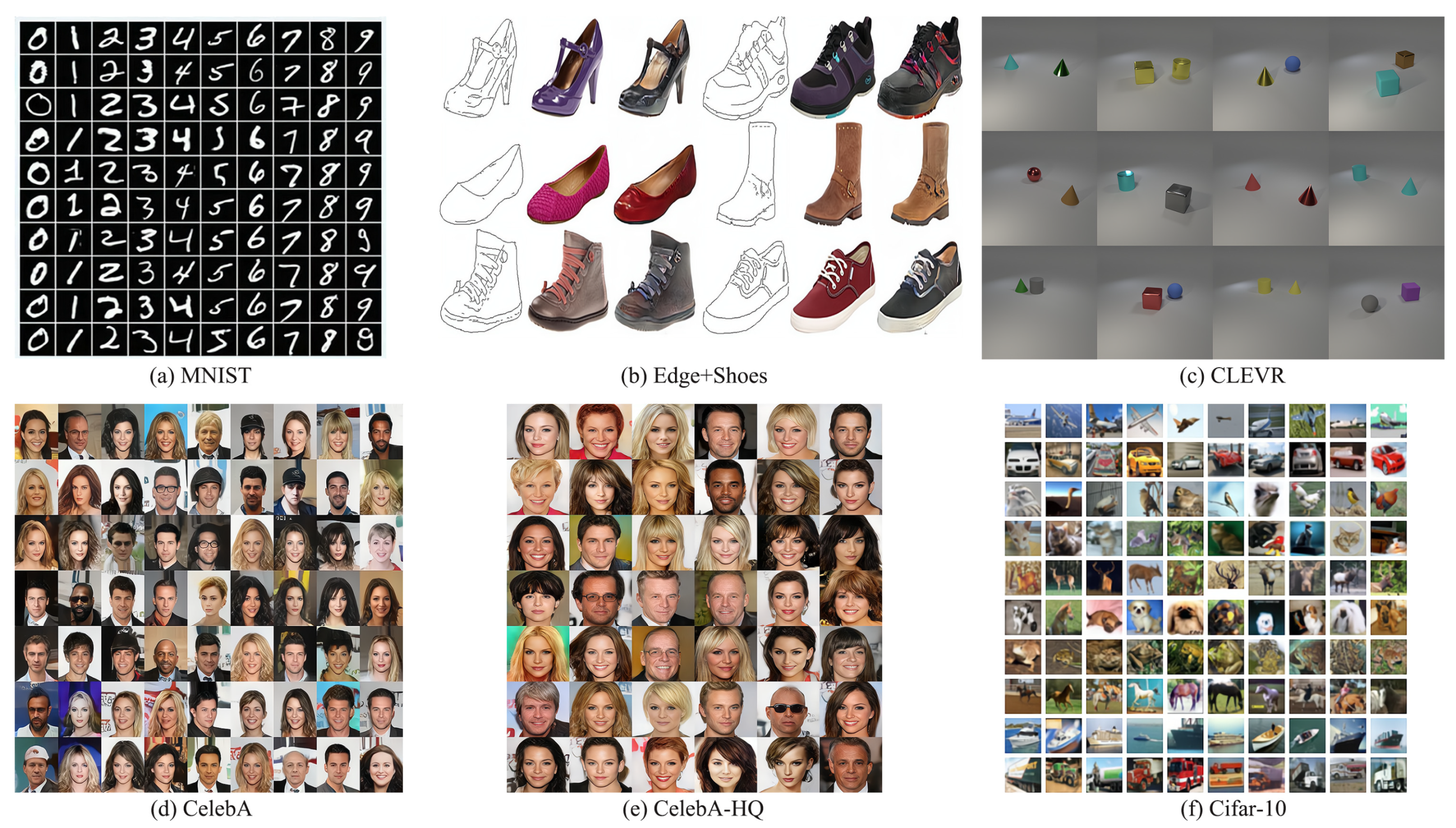
The MNIST dataset was sourced from a mixture of two datasets, one handwritten by employees from the Census Bureau and one handwritten by high school students; this dataset had 60,000 training samples and the rest 10,000 were test samples, with each image being a single number from 0 to 9. Example images of the dataset is shown in Figure 2a.
The Cifar-10 dataset has 60,000 images, which are 32 × 32 and divided into ten categories with 6000 images in each category. Example images of the dataset is shown in Figure 2f.
CelebA is the open dataset of the Chinese University of Hong Kong, containing 202,599 images of 10,177 celebrity identities. Each image is annotated with 40 attributes. Example images of the CelebA dataset are shown in Figure 2d. CelebA-HQ is a high-quality face image of CelebA, consisting of 30,000 images. In the experiments on the CelebA-HQ dataset, we mainly use 256 × 256 size images. Example images of the CelebA-HQ dataset are shown in Figure 2e.
The CLEVR dataset is known as Compositional Language and Elementary Visual Reasoning. CLEVR contains 100,000 rendered images and approximately 1 million automatically generated questions, of which 853,000 are mutually exclusive. Example images of the dataset are shown in Figure 2c.
Edge + Shoes is a simple dataset. This is a large dataset that includes 50,025 images. These images are divided into four categories: shoes, sandals, flip-flops, and boots. Example images of the dataset are shown in Figure 2b.
4.2. Resistance Model Collapse
In this part, we do not directly use the loss of the Formula (15), but instead use the and parameters in the loss, which are used in the model, specifically using the part of the algorithm presented in Appendix A.2. The specific use of and in the model is in Algorithm A1. The reason for doing so is to optimize the current GAN model and make the basis for the disentanglement.
We run real image generation experiments on different datasets: MNIST, CIFAR-10, and CelebA. It has been demonstrated experimentally that our approach is general to some generative models.
We train all models for 25,000 iterations, and in each iteration, we pass the parameters in the generator to the discriminator at a certain frequency. At inference, we generate 10k samples from each training model and measure these two metrics. We report in Table 1 the average scores (IS) of the images generated on the MNIST dataset [34], and p means p-value of the statistical significance. As shown in Table 1, ours outperforms the other methods. We divided the original training datasets into two parts to measure their IS. Since the IS values calculated by different sample segmentation methods are different (this is because the calculation of IS needs to calculate the two groups of pictures, and the segmentation method determines the difference of the calculated values), so it is not given in the Table 1 and Table 2. The first p-value is determined from the IS means of the original method and the IS means within the original training datasets. The second p-value (p (ours)) is determined by the IS means of our method and the IS means of the original training datasets. These two p-values compare the IS means of the method before and after the improvement with the original training datasets. Taking = 0.001 as the judging criterion, our results show that the difference between the IS means of the images generated by our GANs network and the IS means of the original datasets are statistically significant.
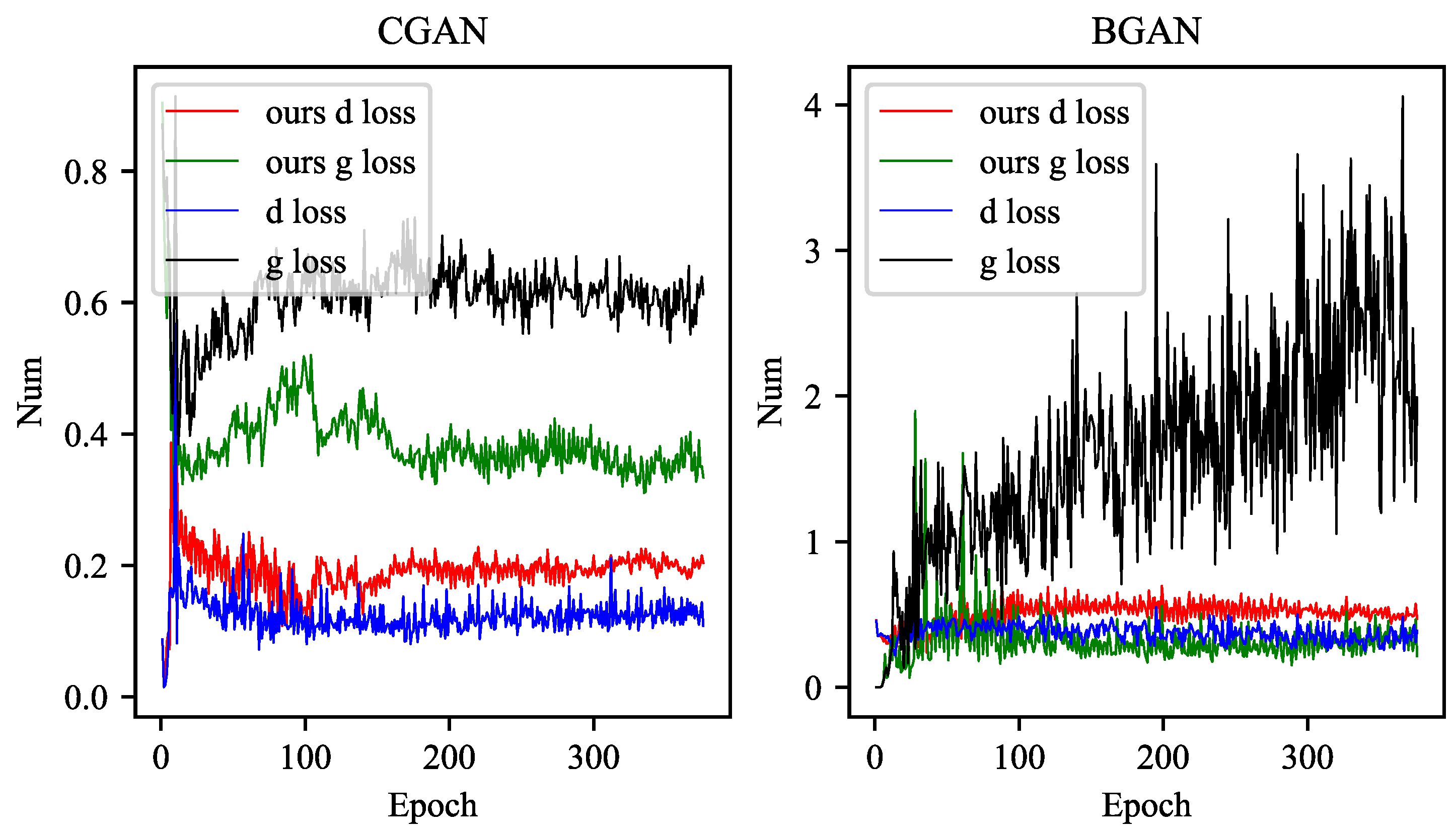
The experimental results in Figure 3 show that the BGAN [36] model modified by our method has a Discriminator closer to 0.5 than the original BGAN [36], and the fluctuation is much smaller than that of the model without our method. At the same time, it has faster convergence and stability.
Figure 3 shows that our improved model is more stable than the original one in CGAN [31]. For more experimental results of the loss function curves refer to Appendix B.
After training all models for 100 K iterations, we evaluated the method on CIFAR-10. Unlike MNIST, the models in this dataset are difficult to handle. We need to evaluate color images, and the contents of pictures are more diverse. That is why we use two different metrics (IS and FID) for inferring the generator quality and diversity. As shown in Table 2, our method consistently outperforms all other methods on these two metrics.
We trained on the standard CIFAR-10 dataset and used the Inception v3 image classification model to calculate the similarity of statistical aspects of computer vision features to measure the similarity of the two datasets. As shown in Table 3, our method generates FID values with the optimal ones.
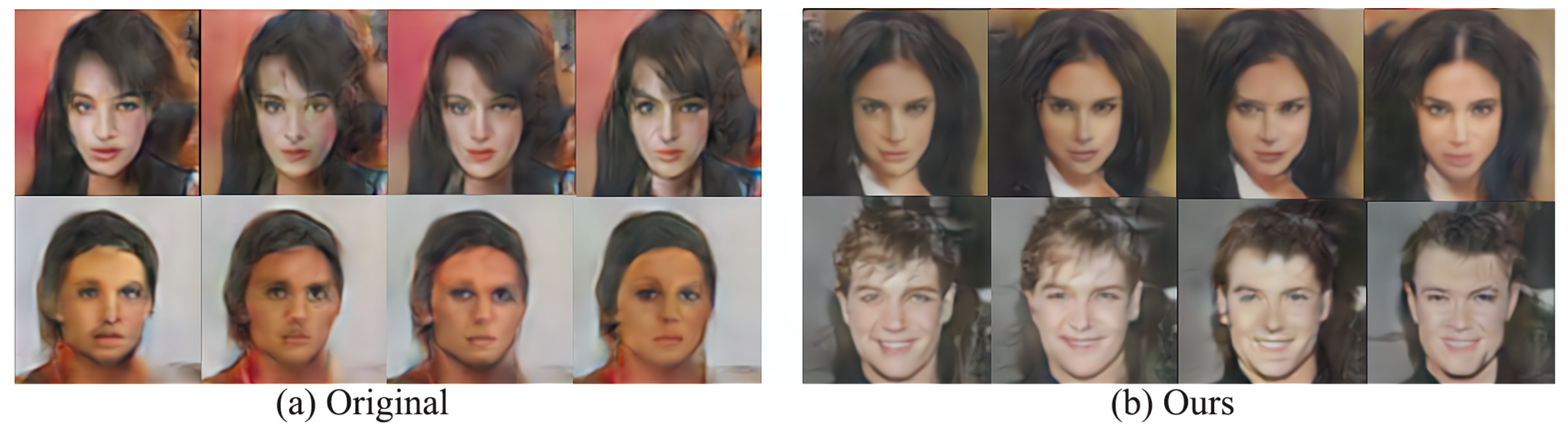
In Figure 4, we compare the image generated in CelebA by the original DCGAN [33] and ours. We reduced the image size of CelebA to 96 × 96 to speed up the training process for faster results. The generated image is also in the size of 96 × 96. Compare our method with the method before improvement in Figure 4, it is not difficult to find that the image face generated by the original DCGAN [33] is blurry and distorted, and the hairstyle has fewer changes in shape and eyebrow shape. Figure 4b is generated by our method, which is improved on the original basis, it has better clarity and diversity. In Figure 4, the faces of the upper character (with a variety of hairstyles) in the (b) pictures are more clear, and the forehead hair of the task in the lower (b) pictures are from long to short, showing the diversity of hairstyles. The image generated by our method also has fewer facial artifacts than the images on the original DCGAN (a).
4.3. Disentanglement Experiments
4.3.1. Qualitative Experiments
In this subsection, we compare Hessian penalty [13] and OroJaR [14] with our method. After adding the and parameters in the model training, some cases will bring more serious attribute entanglement, so we add the Equation (15) to disentanglement and compare the current best results.
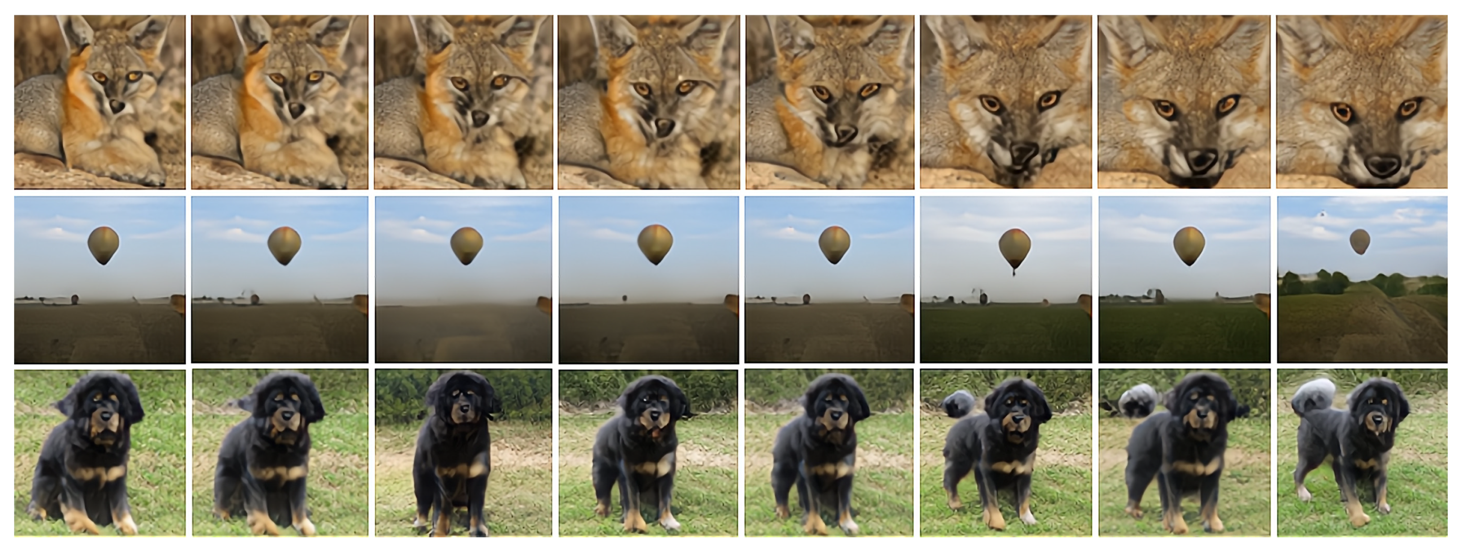
Figure 5 shows experiments been done on fox, balloons, and Tibetan mastiffs on ImageNet. We moved the images in Z-space for each row. Z-space represents the sample space of latent variables.The input position of the Z-space refers to Figure 1. Through the change of the Z-space parameters, the model generates a series of pictures, as shown in Figure 5. The role of these diagrams is explained next. The first line in Figure 5 shows the enlargement of the fox’s face, after disentanglement, the Z-space parameters can control the distance between the object and the lens; the second line shows the separation and change of the background, we separate the balloon from the background, separate the balloon property, and change the background without changing this property, and the third line shows the separation and action of the foreground object (the Tibetan mastiff gradually stands up). The foreground object is a Tibetan mastiff, and the background is grass. By selecting the direction of the Z-space, the foreground object can make actions without changing the background.
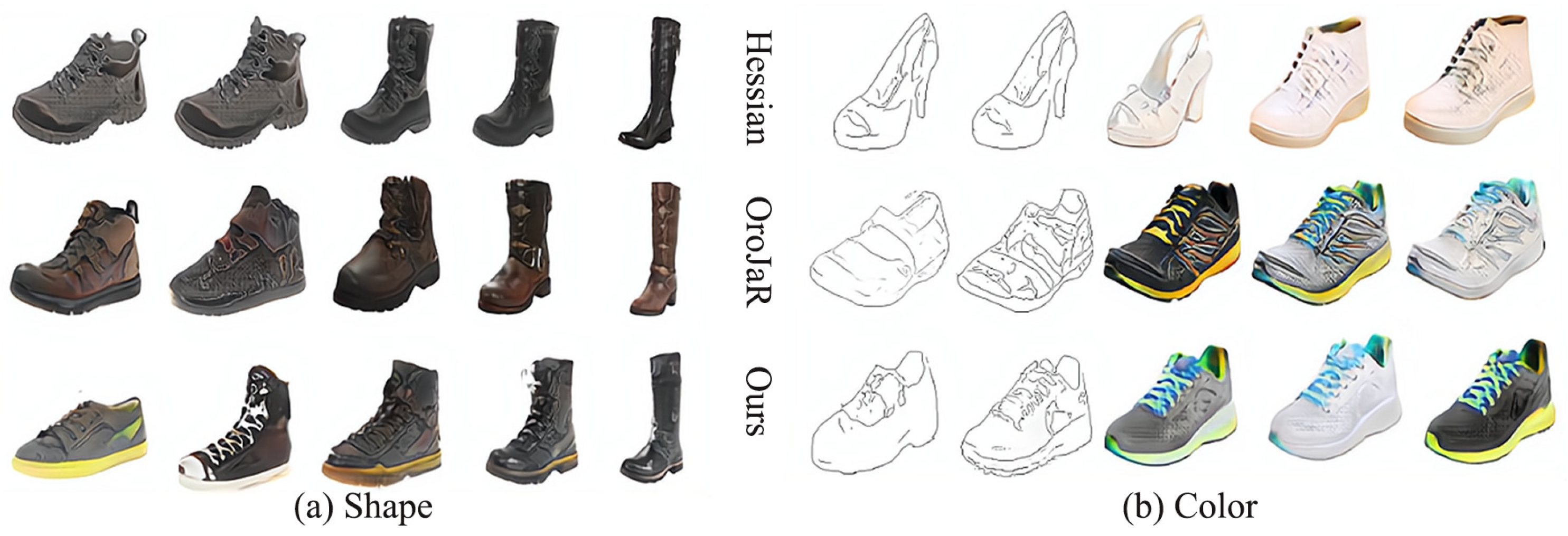
In Figure 6, we present the experimental results of our model on the Edge + Shoes dataset. We choose the two interpretable dimensions of shoe color and style to display, with each row corresponding to one interpretable dimension. Figure 6 shows OroJaR [14], Hessian penalty [13], and our method learned the two separated changes, i.e., style and shape of shoes (the first row of each sub-image is generated by the Hessian method [13], the middle row by the OroJaR [14] method, and the last row is produced by our method). Subfigure (a) shows the performance of different methods in disentangling shape entanglement, and our method covers more shapes. Subfigure (b) shows different methods in disentangling color in terms of entanglement performance; Hessian penalizes [13] to generate a single color of the image, and OroJaR [14] generates a serious color coupling of shoe images. Our method covers more colors, and the independence of colors is better than others.
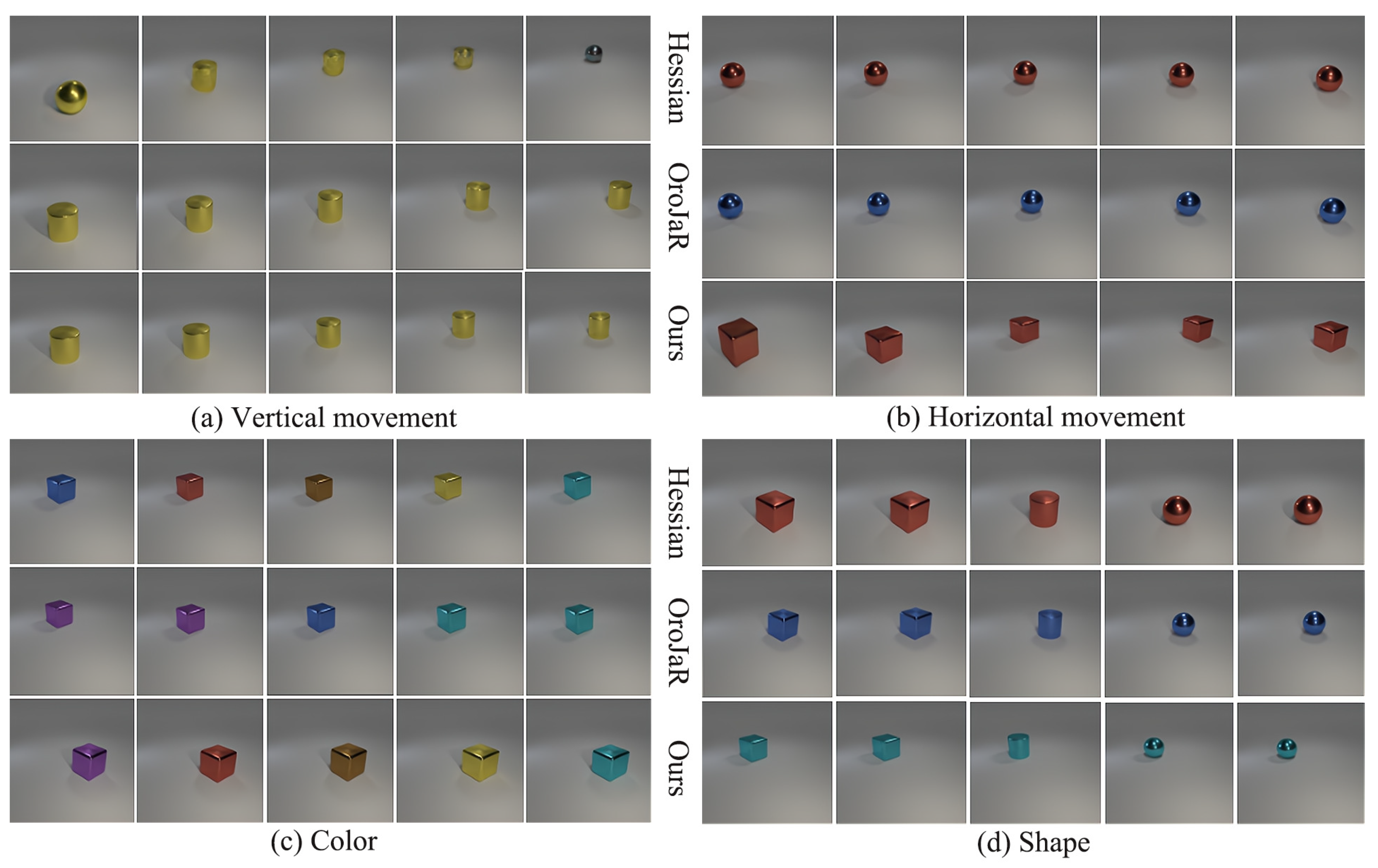
Figure 7 shows the results on the CLEVR simple dataset. Our method is able to separate the potential space effectively. We show the four scoring dimensions of x axial shift, y axial shift, color, and shape. Hessian penalty learning independently controls the vertical and horizontal axial position of the object (first row of each subplot of Figure 7). However, the shape is not controlled during the vertical movement. OroJaR [14] successfully separates the horizontal, shape factors in CLEVR (second row of each subfigure of Figure 7), but shows a tendency to shift toward the horizontal in the separation of the vertical movement. Lastly, our method can successfully separate independent axial shifts and colors in CLEVR (the third row of each subplot of Figure 7).
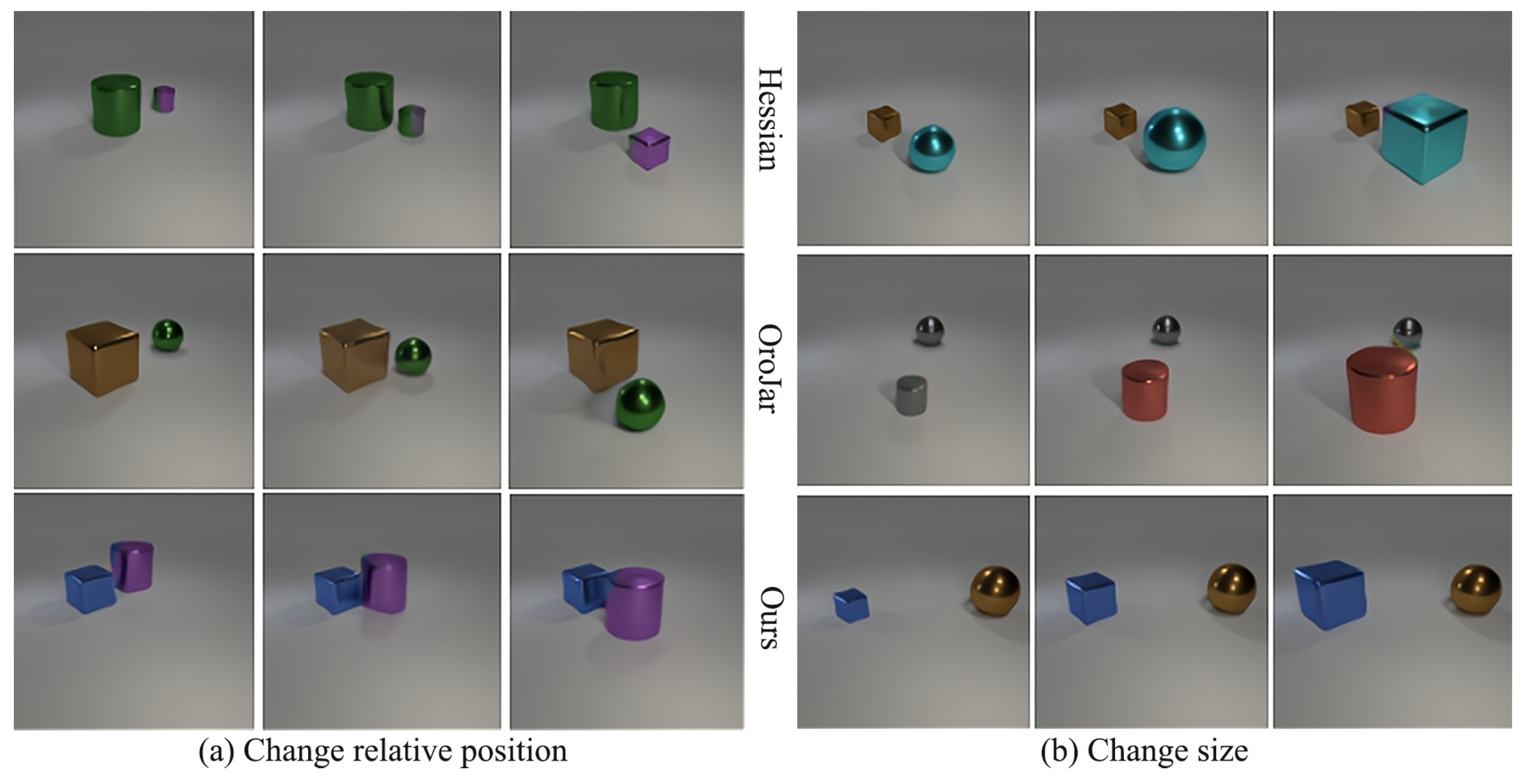
Figure 8 shows the comparison on the CLEVR complex dataset. Here we show the relative position as a factor. From Figure 8, we can conclude: (1) The Hessian penalty does not perform well in the relative positions of two objects, and when the Hessian penalty changes the relative positions of two objects, the shapes or colors of these two objects change at the same time (first row of each subplot of Figure 8). (2) OroJaR [14] changes its shape when the relative position changes (second row of each subfigure of Figure 8). (3) Our method does not change shape and color when the relative position changes (third row of each subfigure of Figure 8).
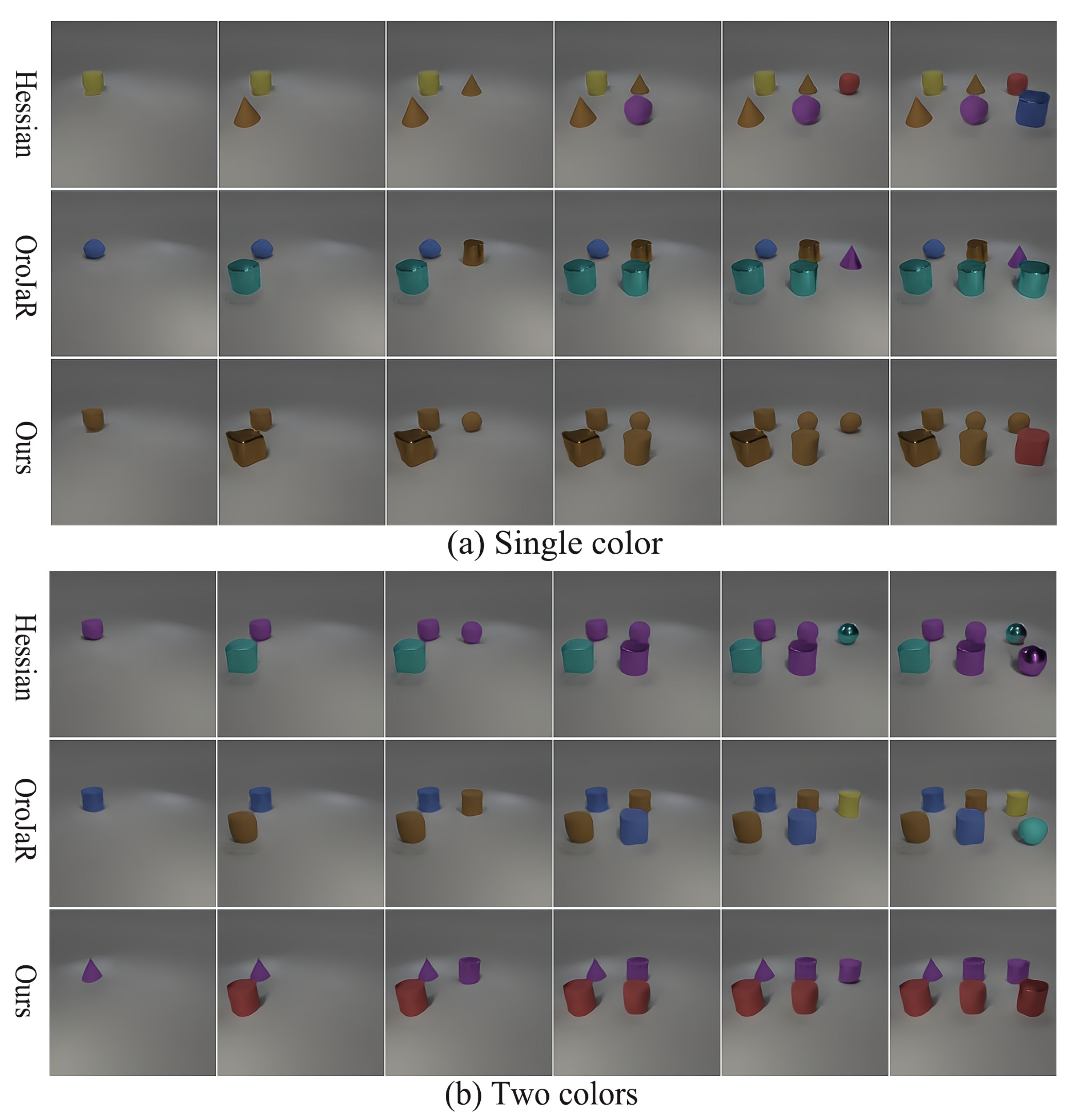
In Figure 9, subfigure (a) shows that, in the case of adding objects, it tries to keep the color properties unchanged. Subfigure (b) shows that it is possible to add objects and keep their shape properties in the case of two colors. The graphs in the first row of subgraphs (a) and (b) in Figure 9 are generated by Hessian penalty [13], the graphs in the second row are generated by OroJaR [14], and the graphs in the third row are generated by our method. The graphs generated by the Hessian penalty [13] appear in five colors as the objects gradually increase from one to six. The graphs generated by OroJaR [14] appear in four colors. Our method emerges in two colors. Although none of the three methods achieves the best-case scenario of producing only one color, our method is more advantageous in color preservation when adding objects. In subgraph (b), the graphs generated by Hessian penalty [13] appear in two colors and two shapes, and the graphs generated by OroJaR [14] appear in more than two colors. However, the shape remains relatively stable (five cylinders in a row) compared to the previous two methods. The shape-preserving effect of our method is also stable in two colors.
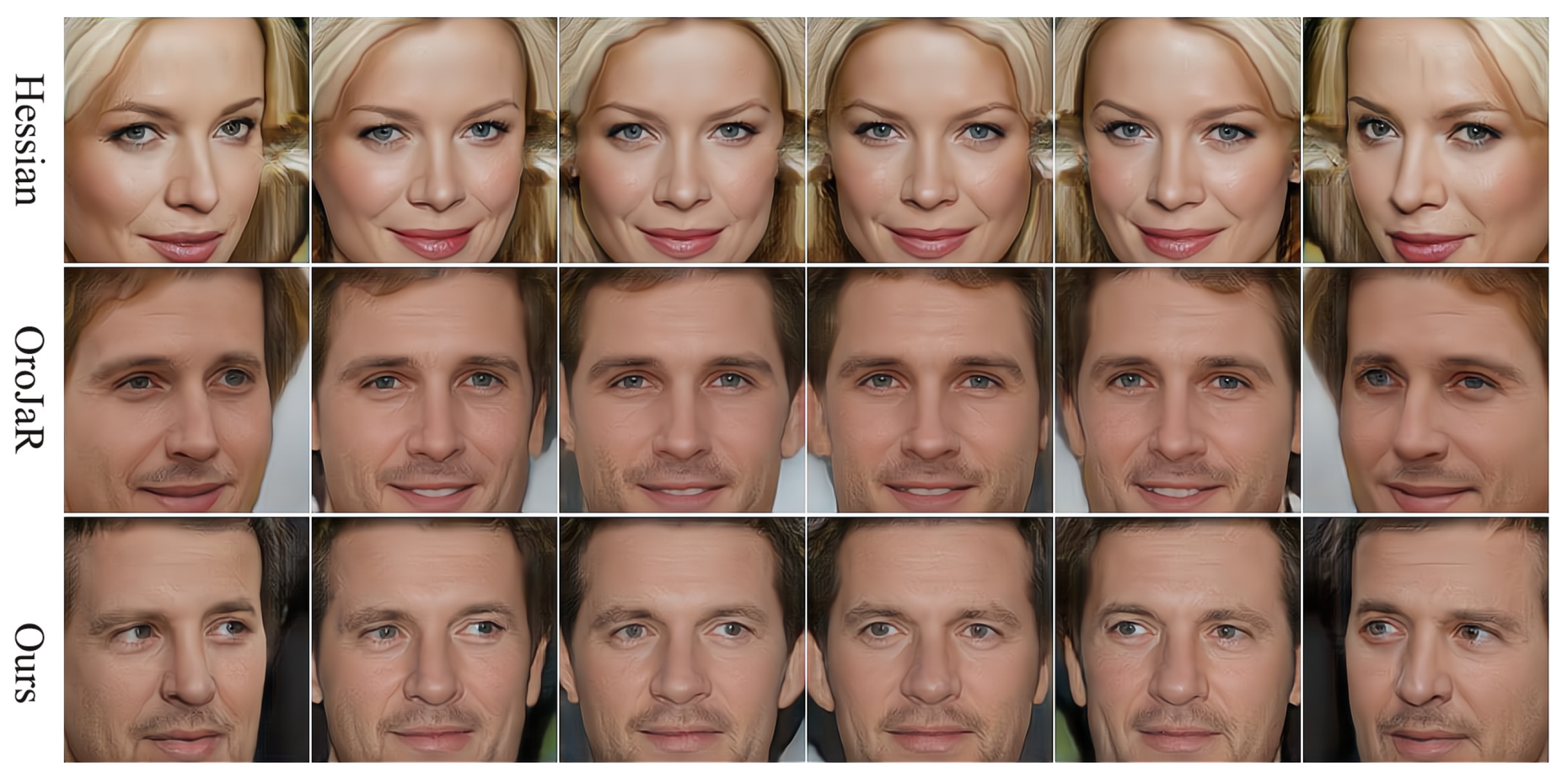
We conduct disentanglement experiments on the CelebA-HQ dataset and compare the performance of Hessian penalty [13], OroJaR [14], and our method on face rotation. In Figure 10, the graphs in the first row are generated by Hessian penalty [13], the graphs in the second row are generated by OroJaR [14], and the graphs in the third row are generated by our method. The properties required for disentanglement are independent of each other. When one property is changed, the other properties remain unchanged. From the comparison in Figure 10, it can be found that, when the Hessian penalty [13] modifies the rotation attribute, the eyes of the characters in the figures always look towards the camera and do not rotate with the characters, resulting in disentanglement. Moreover, artifacts are created at the edges in the first row of images. The eyes of the OroJaR [14] method in the second line rotate with the picture character, but when only controlling the rotation of the character’s avatar, the mouth shape of the second line changes uncontrollably (from normal to slightly flared). The third row shows the performance of our method on face rotation. Our method achieves the rotation of the eyes and the character together, and the mouth shape remains unchanged, which cannot be achieved by the first two methods.
4.3.2. Quantitative Evaluation
In this subsection, we compare our method quantitatively with some models. Referring to [13], we use perceptual path length (PPL) [1], Frechet inception distance (FID) [30], and variance predictability disentanglement measure (VP) [45] as quantitative metrics. Lower FID and PPL are better, and higher VP is better.
As can be seen from Table 4, our method has obtained some better results on some datasets, which indicates that our method has a better disentanglement representation.
4.4. Limitation and Discussion
Our proposed method performs well on mode collapse mitigation and disentanglement, scoring higher than other methods on the test dataset. However, our mode collapse mitigation and disentanglement methods need to be used separately and cannot be combined with one model simultaneously. Our approach to mode collapse mitigation focuses on making the discriminator and generator of the generative adversarial network interact with weights, and discriminator and generator can achieve better results in this way. More features will also bring the coupling of properties, making it impossible to achieve the expected disentanglement effect after adding the disentanglement loss. In the future, applying both mode collapse mitigation and disentanglement methods to the model is a considered direction for improvement.
5. Conclusions
In this work, we introduced a new method to train generative networks. We apply our method to generative adversarial training by learning disentanglement representations. We train the generator to optimize this disentanglement representation through loss or hyperparameters. Our framework accumulates many desirable properties: it does not require any additional trainable parameters, it operates in an unsupervised environment, and it outperforms state-of-the-art methods in some image datasets. Moreover, our method exhibits stable adversarial training, and our method allows embedding any variant of the GAN model. In the future, the neural radiance field can be combined with existing models to achieve a better disentanglement representation.
Author Contributions
Conceptualization, Y.Q., G.Y. and X.F.; methodology, Y.Q.; software, X.F.; validation, Y.Q., G.Y. and X.F.; formal analysis, Y.Q. and G.Y.; investigation, Y.Q. and G.Y.; resources, X.F.; data curation, G.Y.; writing—original draft preparation, Y.Q. and G.Y.; writing—review and editing, X.F.; visualization, G.Y. and X.F.; supervision, X.F.; project administration, Y.Q.; funding acquisition, X.F. All authors have read and agreed to the published version of the manuscript.
Funding
This research was funded by The School Foundation of Anhui University of Science and Technology grant number No:2021CX2102.
Institutional Review Board Statement
Not applicable.
Informed Consent Statement
Not applicable.
Data Availability Statement
The code is available in https://github.com/mathinabel/HessianAndJocbian, accessed on 26 April 2022.
Acknowledgments
This research has been supported by the School Foundation of Anhui University of Science and Technology.
Conflicts of Interest
The authors declare no conflict of interest. The funders had no role in the design of the study; in the collection, analyses, or interpretation of data; in the writing of the manuscript, or in the decision to publish the results.
Abbreviations
The following abbreviations are used in this manuscript:
| GAN | Generative Adversarial Networks |
| D | Discriminator |
| G | Generator |
| KL | Kullback-Leibler divergence |
| FID | Fréchet Inception Distance |
| IS | Inception Score |
Appendix A. Supplementary Theory
Appendix A.1. Eagle Dove Game
Consider the later stage of the training process, when the Generation distribution of G is almost the same as the original distribution, the corresponding equilibrium will be similar. At this time, DG and the corresponding equilibrium are likely interlaced and matched, so only this is difficult for such a theory to describe the DG game process completely. Thus, this model was explained from the perspective of game theory. “Eagle Dove Game” is a classic game model. The basic description of this model is that, in a particular game environment, both sides of the game have the right to be an eagle and a dove. If both sides of the game choose eagles, then they go out to discount the benefits, and the remaining benefits are divided equally. If one party chooses the dove and the other side still chooses the eagle, the other side will win. If both sides choose the doves, compared to the eagle, they could evenly split the gains without losing the competitive discount. Then, the resulting payout matrix is as Table A1:

Table A1.
A result payout matrix of Eagle Dove Game.
| Strategy | Eagle | Dove |
|---|---|---|
| Eagle | S = (v − c)/2, S = (v − c)/2 | T = v, P = 0 |
| Dove | P = 0, T = v | R = v/2, R = v/2 |
Table A1 shows the conclusion that the abilities of both parties in the game are the same, v is the benefit and v is the conflict cost paid by both parties, S is the benefit of both parties when both parties choose eagle strategy, T is the benefit of both parties when both parties choose eagle dove strategy, P is the benefit of both parties when both parties choose eagle dove strategy, and R is the benefit of both parties when both parties choose eagle strategy. If the skills of both parties are the same, then the choice is good, but just like the relationship between the Discriminator and the Generator, the ability between the two parties in the game is a big gap. Suppose the skills of the two parties differ significantly, in that case, the strategy chosen by the two parties, the Discriminator and Generator must be affected by the ratio of the capabilities of the two parties. When the two parties fight at this time, the obtained gain is related to the difference in the strength of the two parties. It proves that the better Generators trained initially and the Discriminators with average learning speed cannot effectively train the ideal results. Let the ability ratio of the two parties involved in the game to the degree of asymmetry be k: (1 − k), then if the conflict loss is greater than the cooperation gain, the payment matrix is shown in Table A1 can be converted to Table A2:
Table A2.
A new result payout matrix of Eagle Dove Game.
| Strategy | Eagle | Dove |
|---|---|---|
| Eagle | (v − c)/4k, (v − c)/4k | (v, 0) |
| Dove | (0, v) | (kv, (1 − k)v) |
The reason for multiplying by 1/4 in Table A2 is that, when k is 0.5, the model degenerates to a classic eagle–dove game. Under the change of payment matrix, neither party in the game has a purely strict dominant strategy equilibrium. Assuming that the Generator’s frequency adopting the dove strategy is x, and the Discriminator adopts the dove strategy as y, then correspondingly, the frequency of the Generator adopts the eagle strategy is 1 − x, and Discriminator adopts the dove strategy as expected 1 − y. Then, according to Table A2, it shows that the expected return of the Generator choosing the eagle strategy is: The expected return of the Generator’s choice of dove strategy is: . The Discriminator chooses the expected return of the eagle strategy as: . The expected return of the Discriminator’s dove strategy choice is: . Then the average expected return of the corresponding Generator is: . In the same way, the average expected return of the corresponding Discriminator is: . Let , , then, the Nash equilibrium can be solved as:
. In this way, we obtain the parameters about DG: , . These parameters can provide us with important hyperparameters initialization guidance in subsequent actual experiments.
Appendix A.2. Model Architecture
In our model, the DG process is regarded as two parts. One part is to update the Generator’s weights; the other part is to update the Discriminator’s weights. The direction of the Generator and the Discriminator on the saddle point is opposite, the point that finally meets is the saddle point, which is also the Nash equilibrium point of the game. Updating the weights of the Generator and the Discriminator will cause their updated weight direction to be opposite the original direction simultaneously. Its pseudo-code refers to Algorithm A1.
| Algorithm A1 Our gradient descent training of GAN |
| Require: Images in datasets; k, , ; k is a default GAN training steps, is D interaction frequency, is D interaction frequency; Ensure: Distribution of target datasets; for training iterations do for k steps do Take samples from noise prior. Take examples from data generating distribution. Update the D. for steps do Update the G. end for Take examples from data generating distribution. for steps do Update the G. end for Take examples from data generating distribution. end for Take noise samples from noise prior. for steps do Take examples from data generating distribution. end for Update the G. end for |
Appendix B. Other Experiments
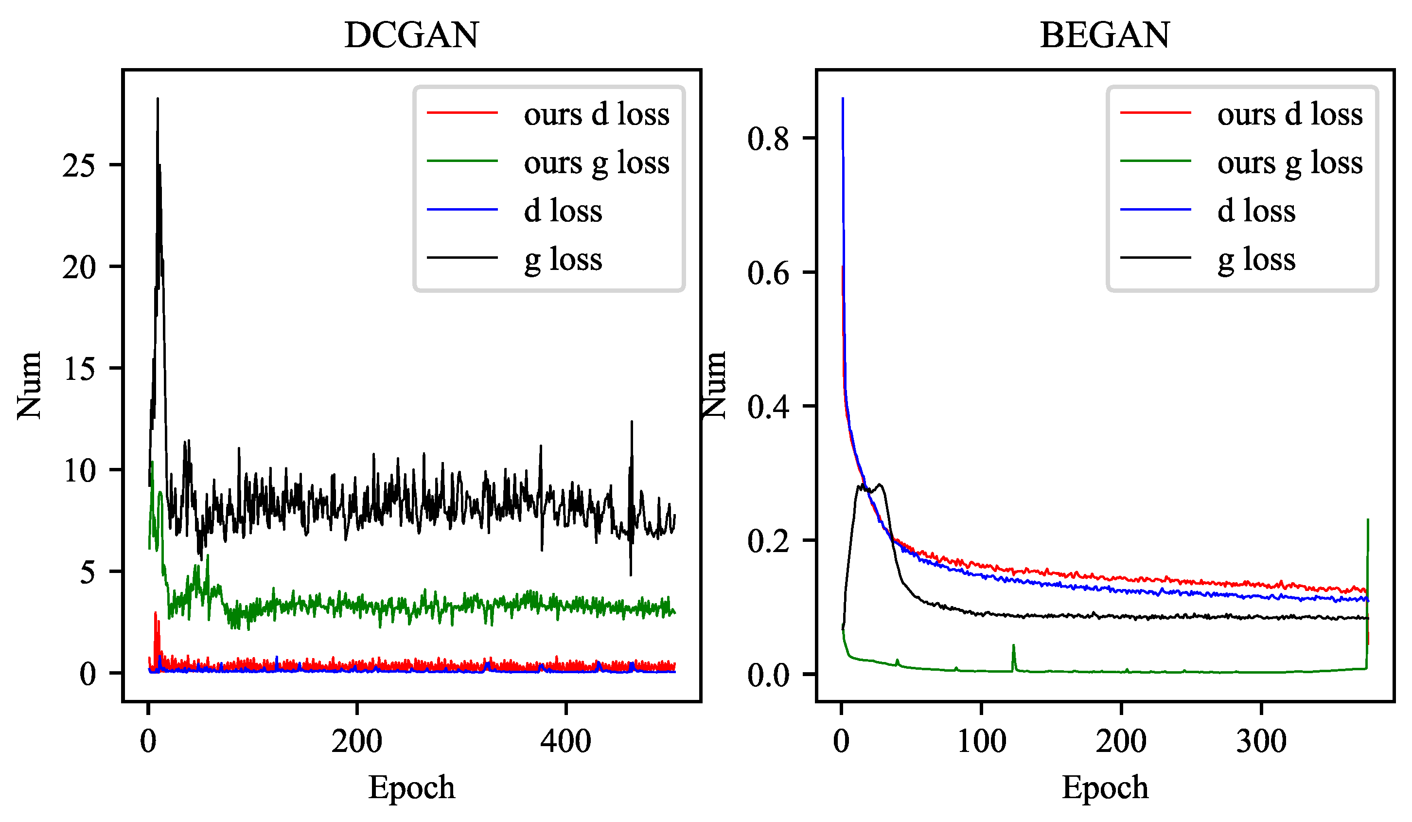
Both the discriminator and generator of DCGAN [33] use a convolutional neural network to replace the multi-layer perceptron in GAN, and use convolution and deconvolution to replace the pooling layer. The output layer of the generator uses the Tanh activation function, and the other layers use RELU, the discriminator LeakyReLU activation function is used for all layers of. After the network is added to our method, Figure A1 shows that the generator fluctuation of the network is significantly reduced, and the numerical distance between the network and the discriminator is also getting closer.

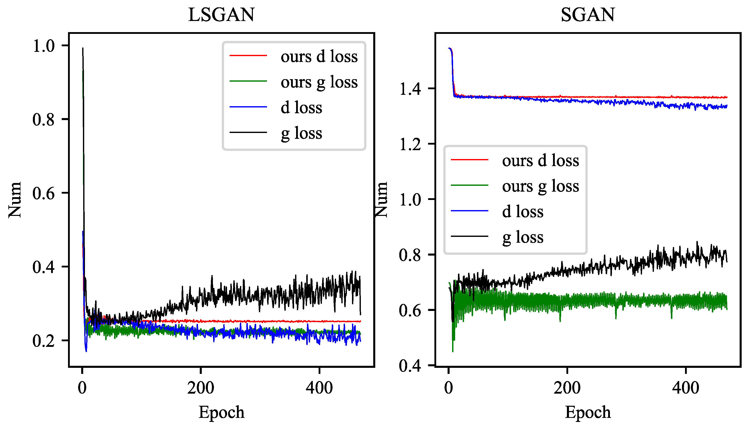
In Figure A1, we found that our method is not very effective for the network of the GAN network generator that uses the loss of Wasserstein distance, but in the actual training process, it can reach the training completion standard at a faster speed, so that we need early stop to finish training.
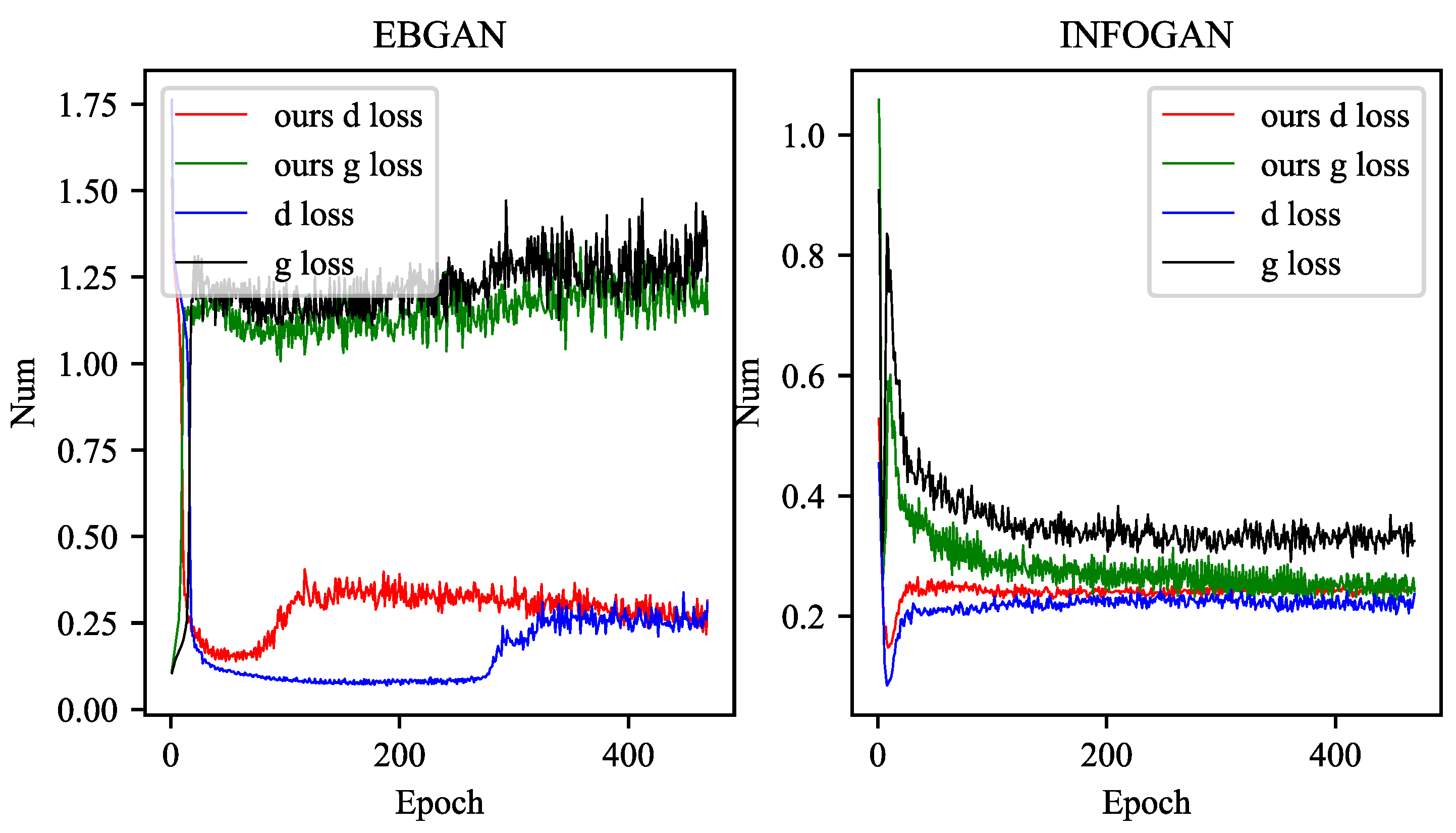
A pull-away term was proposed to prevent Generator from generating the same image. In Figure A2, our method has smaller oscillation and convergence on this EBGAN [10], and the time to reach stable generation is also shorter.
INFOGAN [32] divides Z into fixed distribution noise and c some hidden variable information on the basis of DC-GAN. In Figure A2, after adding our method, DG converges faster and gets closer.


References
- Karras, T.; Laine, S.; Aila, T. A Style-Based Generator Architecture for Generative Adversarial Networks. IEEE Trans. Pattern Anal. Mach. Intell. 2020, 43, 4217–4228. [Google Scholar] [CrossRef] [PubMed] [Green Version]
- Brock, A.; Donahue, J.; Simonyan, K. Large Scale GAN Training for High Fidelity Natural Image Synthesis. In Proceedings of the International Conference on Learning Representations, Vancouver, BC, Canada, 30 April–3 May 2018; pp. 4389–4399. [Google Scholar] [CrossRef]
- Choi, Y.; Choi, M.; Kim, M.; Ha, J.W.; Kim, S.; Choo, J. Stargan: Unified generative adversarial networks for multi-domain image-to-image translation. In Proceedings of the IEEE Conference on Computer Vision and Pattern Recognition, Salt Lake City, UT, USA, 18–23 June 2018; pp. 8789–8797. [Google Scholar] [CrossRef] [Green Version]
- Choi, Y.; Uh, Y.; Yoo, J.; Ha, J.W. Stargan v2: Diverse image synthesis for multiple domains. In Proceedings of the IEEE/CVF Conference on Computer Vision and Pattern Recognition, Seattle, WA, USA, 13–19 June 2020; pp. 8185–8194. [Google Scholar] [CrossRef]
- Karras, T.; Laine, S.; Aittala, M.; Hellsten, J.; Lehtinen, J.; Aila, T. Analyzing and improving the image quality of stylegan. In Proceedings of the IEEE/CVF Conference on Computer Vision and Pattern Recognition, Seattle, WA, USA, 13–19 June 2020; pp. 8107–8116. [Google Scholar] [CrossRef]
- Tolstikhin, I.; Gelly, S.; Bousquet, O.; Simon-Gabriel, C.J.; Schölkopf, B. AdaGAN: Boosting generative models. In Proceedings of the International Conference on Neural Information Processing Systems, Long Beach, CA, USA, 4–9 December 2017; pp. 5430–5439. [Google Scholar] [CrossRef]
- Nguyen, T.D.; Le, T.; Vu, H.; Phung, D. Dual discriminator generative adversarial nets. In Proceedings of the International Conference on Neural Information Processing Systems, Long Beach, CA, USA, 4–9 December 2017; pp. 2667–2677. [Google Scholar] [CrossRef]
- Arjovsky, M.; Chintala, S.; Bottou, L. Wasserstein generative adversarial networks. In Proceedings of the International Conference on Machine Learning, Sydney, Australia, 6–11 August 2017; pp. 214–223. [Google Scholar] [CrossRef]
- Mao, X.; Li, Q.; Xie, H.; Lau, R.Y.; Wang, Z.; Paul Smolley, S. Least squares generative adversarial networks. In Proceedings of the IEEE International Conference on Computer Vision, Honolulu, HI, USA, 21–26 July 2017; pp. 2794–2802. [Google Scholar] [CrossRef] [Green Version]
- Zhao, J.; Mathieu, M.; LeCun, Y. Energy-based generative adversarial networks. In Proceedings of the International Conference on Learning Representations, Toulon, France, 24–26 April 2017; pp. 1682–1693. [Google Scholar] [CrossRef]
- Gurumurthy, S.; Kiran Sarvadevabhatla, R.; Venkatesh Babu, R. Deligan: Generative adversarial networks for diverse and limited data. In Proceedings of the IEEE Conference on Computer Vision and Pattern Recognition, Honolulu, HI, USA, 21–26 July 2017; pp. 166–174. [Google Scholar] [CrossRef] [Green Version]
- Shen, Y.; Zhou, B. Closed-form factorization of latent semantics in gans. In Proceedings of the IEEE/CVF Conference on Computer Vision and Pattern Recognition, Online, 19–25 July 2021; pp. 1532–1540. [Google Scholar] [CrossRef]
- Peebles, W.; Peebles, J.; Zhu, J.Y.; Efros, A.; Torralba, A. The hessian penalty: A weak prior for unsupervised disentanglement. In Proceedings of the Computer Vision–ECCV 2020: 16th European Conference, Glasgow, UK, 23–28 August 2020; Springer: Berlin/Heidelberg, Germany, 2020; pp. 581–597. [Google Scholar] [CrossRef]
- Wei, Y.; Shi, Y.; Liu, X.; Ji, Z.; Gao, Y.; Wu, Z.; Zuo, W. Orthogonal Jacobian Regularization for Unsupervised Disentanglement in Image Generation. In Proceedings of the IEEE/CVF International Conference on Computer Vision, Online, 19–25 July 2021; pp. 6721–6730. [Google Scholar] [CrossRef]
- Creswell, A.; Bharath, A.A. Denoising adversarial autoencoders. IEEE Trans. Neural. Netw. Learn. Syst. 2018, 30, 968–984. [Google Scholar] [CrossRef] [PubMed] [Green Version]
- Odena, A.; Olah, C.; Shlens, J. Conditional image synthesis with auxiliary classifier gans. In Proceedings of the International Conference on Machine Learning, Sydney, Australia, 6–11 August 2017; pp. 2642–2651. [Google Scholar] [CrossRef]
- Ghasedi Dizaji, K.; Wang, X.; Huang, H. Semi-supervised generative adversarial network for gene expression inference. In Proceedings of the ACM SIGKDD International Conference on Knowledge Discovery & Data Mining, London, UK, 19–23 August 2018; pp. 1435–1444. [Google Scholar] [CrossRef]
- Liu, M.; Deng, J.; Yang, M.; Cheng, X.; Xie, T.; Deng, P.; Wang, X.; Liu, M. Express Construction for GANs from Latent Representation to Data Distribution. Appl. Sci. 2022, 12, 3910. [Google Scholar] [CrossRef]
- Abdal, R.; Zhu, P.; Mitra, N.J.; Wonka, P. Styleflow: Attribute-conditioned exploration of stylegan-generated images using conditional continuous normalizing flows. ACM. Trans. Graph. 2021, 40, 1–21. [Google Scholar] [CrossRef]
- Collins, E.; Bala, R.; Price, B.; Susstrunk, S. Editing in style: Uncovering the local semantics of gans. In Proceedings of the IEEE/CVF Conference on Computer Vision and Pattern Recognition, Seattle, WA, USA, 13–19 June 2020; pp. 5771–5780. [Google Scholar] [CrossRef]
- Goetschalckx, L.; Andonian, A.; Oliva, A.; Isola, P. Ganalyze: Toward visual definitions of cognitive image properties. In Proceedings of the IEEE/CVF International Conference on Computer Vision, Seoul, Korea, 27 October–2 November 2019; pp. 5744–5753. [Google Scholar] [CrossRef] [Green Version]
- Jahanian, A.; Chai, L.; Isola, P. On the “steerability” of generative adversarial networks. In Proceedings of the International Conference on Learning Representations, New Orleans, LA, USA, 6–9 May 2019. [Google Scholar] [CrossRef]
- Shen, Y.; Gu, J.; Tang, X.; Zhou, B. Interpreting the latent space of gans for semantic face editing. In Proceedings of the IEEE/CVF Conference on Computer Vision and Pattern Recognition, Seattle, WA, USA, 13–19 June 2020; pp. 9243–9252. [Google Scholar] [CrossRef]
- Goodfellow, I.; Pouget-Abadie, J.; Mirza, M.; Xu, B.; Warde-Farley, D.; Ozair, S.; Courville, A.; Bengio, Y. Generative adversarial nets. Adv. Neural. Inf. Process. Syst. 2014, 63, 139–144. [Google Scholar] [CrossRef]
- Kingma, D.P.; Welling, M. Auto-encoding variational bayes. arXiv 2013, arXiv:1312.6114. [Google Scholar]
- Jeewajee, A.K.; Kaelbling, L. Adversarially-learned Inference via an Ensemble of Discrete Undirected Graphical Models. Adv. Neural. Inf. Process. Syst. 2020, 33, 12660–12672. [Google Scholar] [CrossRef]
- Bertran, M.; Martinez, N.; Papadaki, A.; Qiu, Q.; Rodrigues, M.; Reeves, G.; Sapiro, G. Adversarially learned representations for information obfuscation and inference. In Proceedings of the International Conference on Machine Learning, Long Beach, CA, USA, 9–15 June 2019; pp. 614–623. [Google Scholar]
- Berthelot, D.; Schumm, T.; Metz, L. Began: Boundary equilibrium generative adversarial networks. arXiv 2017, arXiv:1703.10717. [Google Scholar]
- Henzler, P.; Mitra, N.J.; Ritschel, T. Escaping Plato’s cave: 3D shape from adversarial rendering. In Proceedings of the IEEE/CVF International Conference on Computer Vision, Seoul, Korea, 27 October–2 November 2019; pp. 9984–9993. [Google Scholar] [CrossRef] [Green Version]
- Heusel, M.; Ramsauer, H.; Unterthiner, T.; Nessler, B.; Hochreiter, S. Gans trained by a two time-scale update rule converge to a local nash equilibrium. Adv. Neural. Inf. Process. Syst. 2017, 30, 6629–6640. [Google Scholar] [CrossRef]
- Mirza, M.; Osindero, S. Conditional generative adversarial nets. arXiv 2014, arXiv:1411.1784. [Google Scholar]
- Chen, X.; Duan, Y.; Houthooft, R.; Schulman, J.; Sutskever, I.; Abbeel, P. Infogan: Interpretable representation learning by information maximizing generative adversarial nets. In Proceedings of the International Conference on Neural Information Processing Systems, Barcelona, Spain, 5–10 December 2016; pp. 2180–2188. [Google Scholar] [CrossRef]
- Radford, A.; Metz, L.; Chintala, S. Unsupervised representation learning with deep convolutional generative adversarial networks. In Proceedings of the International Conference on Learning Representations, San Diego, CA, USA, 7–9 May 2015; pp. 2203–2212. [Google Scholar] [CrossRef]
- Gulrajani, I.; Ahmed, F.; Arjovsky, M.; Dumoulin, V.; Courville, A. Improved training of wasserstein GANs. In Proceedings of the International Conference on Neural Information Processing Systems, Long Beach, CA, USA, 4–9 December 2017; pp. 5769–5779. [Google Scholar] [CrossRef]
- Liao, Y.; Schwarz, K.; Mescheder, L.; Geiger, A. Towards unsupervised learning of generative models for 3d controllable image synthesis. In Proceedings of the IEEE/CVF Conference on Computer Vision and Pattern Recognition, Seattle, WA, USA, 13–19 June 2020; pp. 5871–5880. [Google Scholar] [CrossRef]
- Hjelm, R.D.; Jacob, A.P.; Che, T.; Trischler, A.; Cho, K.; Bengio, Y. Boundary-seeking generative adversarial networks. In Proceedings of the 6th International Conference on Learning Representations, Vancouver, BC, Canada, 30 April–3 May 2018. [Google Scholar] [CrossRef]
- Wu, Z.; Lischinski, D.; Shechtman, E. Stylespace analysis: Disentangled controls for stylegan image generation. In Proceedings of the IEEE/CVF Conference on Computer Vision and Pattern Recognition, Online, 19–25 July 2021; pp. 12863–12872. [Google Scholar] [CrossRef]
- Härkönen, E.; Hertzmann, A.; Lehtinen, J.; Paris, S. Ganspace: Discovering interpretable gan controls. Adv. Neural. Inf. Process. Syst. 2020, 33, 9841–9850. [Google Scholar] [CrossRef]
- Mildenhall, B.; Srinivasan, P.P.; Tancik, M.; Barron, J.T.; Ramamoorthi, R.; Ng, R. Nerf: Representing scenes as neural radiance fields for view synthesis. In Proceedings of the European Conference on Computer Vision, Glasgow, UK, 23–28 August 2020; pp. 405–421. [Google Scholar] [CrossRef]
- Singh, K.K.; Ojha, U.; Lee, Y.J. Finegan: Unsupervised hierarchical disentanglement for fine-grained object generation and discovery. In Proceedings of the IEEE/CVF Conference on Computer Vision and Pattern Recognition, Long Beach, CA, USA, 15–20 June 2019; pp. 6490–6499. [Google Scholar] [CrossRef] [Green Version]
- Voynov, A.; Babenko, A. Unsupervised discovery of interpretable directions in the gan latent space. In Proceedings of the International Conference on Machine Learning, Congress Center, Vienna, Austria, 13–18 July 2020; pp. 9786–9796. [Google Scholar] [CrossRef]
- Niemeyer, M.; Geiger, A. Giraffe: Representing scenes as compositional generative neural feature fields. In Proceedings of the IEEE Conference on Computer Vision and Pattern Recognition, Online, 19–25 July 2021; pp. 11453–11464. [Google Scholar] [CrossRef]
- Hutchinson, M.F. A stochastic estimator of the trace of the influence matrix for Laplacian smoothing splines. Commun. Stat. Simul. Comput. 1989, 18, 1059–1076. [Google Scholar] [CrossRef]
- Salimans, T.; Goodfellow, I.; Zaremba, W.; Cheung, V.; Radford, A.; Chen, X. Improved techniques for training gans. Adv. Neural. Inf. Process. Syst. 2016, 29, 2234–2242. [Google Scholar] [CrossRef]
- Zhu, X.; Xu, C.; Tao, D. Learning disentangled representations with latent variation predictability. In European Conference on Computer Vision; Springer: Berlin/Heidelberg, Germany, 2020; pp. 684–700. [Google Scholar] [CrossRef]
- Karras, T.; Aila, T.; Laine, S.; Lehtinen, J. Progressive Growing of GANs for Improved Quality, Stability, and Variation. In Proceedings of the International Conference on Learning Representations, Vancouver, BC, Canada, 30 April–3 May 2018; pp. 2581–2592. [Google Scholar] [CrossRef]
Figure 1.
Structure of the network model.

Figure 2.
The datasets used in this article.


Figure 4.
Graph generated without our Network(DCGAN [33]) (a), with ours (b).
Figure 4.
Graph generated without our Network(DCGAN [33]) (a), with ours (b).

Figure 5.
The orthogonal orientation learned on BigGAN [2].
Figure 5.
The orthogonal orientation learned on BigGAN [2].

Figure 6.
Comparison of the disentanglement quality of OroJaR [14], Hessian penalty [13] and our method for Edge + Shoes.

Figure 7.
Comparison with OroJaR [14], Hessian penalty [13], and our method for the disentanglement quality of CLEVR Sample.

Figure 8.
Comparison of disentanglement the quality of the CLEVR complex by our method, Hessian penalty [13], and OroJaR [14].

Figure 9.
Comparison of disentanglement the quality of the CLEVR dataset by our method, Hessian penalty [13] and OroJaR [14] for adding objects.

Figure 10.
Comparison of rotation disentanglement of the CelebA-HQ dataset by our method, Hessian penalty [13], and OroJaR [14].

Table 1.
Score (IS) test on GANs (MNIST).
| GAN | IS (Mean) | IS (Std) | p | IS (Ours Mean) | IS (Ours Std) | p (Ours) |
|---|---|---|---|---|---|---|
| BEGAN [28] | 1.366 | 0.179 | <0.001 | 1.388 | 0.242 | <0.001 |
| BGAN [36] | 1.250 | 0.175 | <0.001 | 1.372 | 0.187 | <0.001 |
| EBGAN [10] | 1.356 | 0.194 | <0.001 | 1.371 | 0.241 | <0.001 |
| INFOGAN [32] | 2.054 | 0.171 | <0.001 | 2.070 | 0.207 | <0.001 |
| CGAN [31] | 2.022 | 0.196 | <0.001 | 2.302 | 0.291 | <0.001 |
| AAE [15] | 2.289 | 0.298 | <0.001 | 1.995 | 0.251 | <0.001 |
| ACGAN [16] | 1.956 | 0.146 | <0.001 | 2.041 | 0.271 | <0.001 |
| LSGAN [9] | 1.404 | 0.183 | <0.001 | 1.363 | 0.139 | <0.001 |
| SGAN [17] | 1.418 | 0.159 | <0.001 | 1.459 | 0.192 | <0.001 |
Table 2.
Score (IS) test on GANs (Cifar-10).
| GAN | IS (Mean) | IS (Std) | p | IS (Ours Mean) | IS (Ours Std) | p (Ours) |
|---|---|---|---|---|---|---|
| BEGAN [28] | 1.735 | 0.215 | <0.001 | 2.005 | 0.236 | <0.001 |
| EBGAN [10] | 1.666 | 0.224 | <0.001 | 1.733 | 0.244 | <0.001 |
| INFOGAN [32] | 1.563 | 0.197 | <0.001 | 1.677 | 0.208 | <0.001 |
| BGAN [36] | 1.822 | 0.203 | <0.001 | 2.932 | 0.221 | <0.001 |
| CGAN [31] | 1.978 | 0.209 | <0.001 | 2.065 | 0.235 | <0.001 |
| AAE [15] | 2.012 | 0.214 | <0.001 | 1.917 | 0.199 | <0.001 |
| ACGAN [16] | 1.771 | 0.231 | <0.001 | 1.871 | 0238 | <0.001 |
| LSGAN [9] | 1.846 | 0.227 | <0.001 | 1.959 | 0.236 | <0.001 |
| SGAN [17] | 1.668 | 0.158 | <0.001 | 2.005 | 0.183 | <0.001 |
Table 3.
Score (FID) test on GANs (Cifar-10).
| GAN | FID (Original) | FID (Ours) |
|---|---|---|
| BGAN [36] | 243.633 | 226.164 |
| BEGAN [28] | 417.625 | 377.760 |
| CGAN [31] | 382.941 | 373.581 |
| AAE [15] | 187.612 | 181.169 |
| ACGAN [16] | 231.143 | 249.174 |
| LSGAN [9] | 149.675 | 133.783 |
| SGAN [17] | 147.770 | 130.251 |
Table 4.
Comparison of different methods on Edge + Shoes and CLEVR.
| Method | Edges + Shoes | CLEVR-Simple | CLEVR-Complex | CLEVR-U | ||||||||
|---|---|---|---|---|---|---|---|---|---|---|---|---|
| PPL (↓) | FID (↓) | VP (↑) | PPL | FID | VP | PPL | FID | VP | PPL | FID | VP | |
| InfoGAN [32] | 2952.2 | 10.4 | 15.6 | 56.2 | 2.9 | 28.7 | 83.9 | 4.2 | 27.9 | 766.7 | 3.6 | 40.1 |
| ProGAN [46] | 3154.1 | 10.8 | 15.5 | 64.5 | 3.8 | 27.2 | 84.4 | 5.5 | 25.5 | 697.7 | 3.4 | 40.2 |
| SeFa [12] | 3154.1 | 10.8 | 24.1 | 64.5 | 3.8 | 58.4 | 84.4 | 5.5 | 30.9 | 697.7 | 3.4 | 42.0 |
| Hessian Penalty [13] | 554.1 | 17.3 | 28.6 | 39.7 | 6.1 | 71.3 | 74.7 | 7.1 | 42.9 | 61.6 | 26.8 | 79.2 |
| OroJaR [14] | 236.7 | 16.1 | 32.3 | 6.7 | 4.9 | 76.9 | 10.4 | 10.7 | 48.8 | 40.9 | 4.6 | 90.7 |
| Ours | 336.79 | 12.5 | 33.7 | 27.6 | 3.3 | 79.1 | 36.3 | 4.3 | 49.3 | 44.1 | 3.3 | 88.3 |
Publisher’s Note: MDPI stays neutral with regard to jurisdictional claims in published maps and institutional affiliations. |
© 2022 by the authors. Licensee MDPI, Basel, Switzerland. This article is an open access article distributed under the terms and conditions of the Creative Commons Attribution (CC BY) license (https://creativecommons.org/licenses/by/4.0/).
Share and Cite
MDPI and ACS Style
Yang, G.; Qu, Y.; Fang, X. Editable Image Generation with Consistent Unsupervised Disentanglement Based on GAN. Appl. Sci. 2022, 12, 5382. https://0-doi-org.brum.beds.ac.uk/10.3390/app12115382
AMA Style
Yang G, Qu Y, Fang X. Editable Image Generation with Consistent Unsupervised Disentanglement Based on GAN. Applied Sciences. 2022; 12(11):5382. https://0-doi-org.brum.beds.ac.uk/10.3390/app12115382
Chicago/Turabian StyleYang, Gaoming, Yuanjin Qu, and Xianjin Fang. 2022. "Editable Image Generation with Consistent Unsupervised Disentanglement Based on GAN" Applied Sciences 12, no. 11: 5382. https://0-doi-org.brum.beds.ac.uk/10.3390/app12115382
Note that from the first issue of 2016, this journal uses article numbers instead of page numbers. See further details here.