The Effect of Porous Media on Wave-Induced Sloshing in a Floating Tank

Featured Application

This research can be applied to sloshing mitigation for LNG vessels and vibration control for offshore structures.

Abstract

Placing porous media in a water tank can change the dynamic characteristics of the sloshing fluid. Its extra damping effect can mitigate sloshing and, thereby, protect the integrity of a liquefied natural gas tank. In addition, the out-of-phase sloshing force enables the water tank to serve as a dynamic vibration absorber for floating structures in the ocean environment. The influence of porous media on wave-induced sloshing fluid in a floating tank and the associated interaction with the substructure in the ambient wave field are the focus of this study. The numerical coupling algorithm includes the potential-based Eulerian–Lagrangian method for fluid simulation and the Newmark time-integration method for rigid-body dynamics. An equivalent mechanical model for the sloshing fluid in a rectangular tank subject to pitch motion is proposed and validated. In this approach, the degrees of freedom modeling of the sloshing fluid can be reduced so the numerical computation is fast and inexpensive. The results of the linear mechanical model and the nonlinear Eulerian–Lagrangian method are correlated. The dynamic interaction between the sloshing fluid and floating body is characterized. The effectiveness of the added porous media in controlling the vibration and mitigating the sloshing response is confirmed through frequency response analysis.

1. Introduction

Fluid–structure interaction (FSI) is the dynamic interaction between a deformable and moveable structure and its surrounding fluid. In recent years, this topic has been a major focus in civil and ocean engineering research because there has been an ongoing interest in exploring mineral and energy resources from the ocean. Various kinds of offshore work platforms have been developed for purposes of petroleum extraction, wind energy, wave energy, and fishing. As they are subject to external loadings from wind, waves, currents, ice, and earthquakes, their dynamics includes complex fluid–structure interactions. Very challenging engineering problems in this area include the seakeeping performance of a ship, as well as the longevity and integrity of the offshore structures arise. For Liquified Natural Gas (LNG) vessels, the rolling motion is of greatest concern because the ambient wave damping is usually too small to limit motion amplitudes, especially when resonance occurs. The strong excitations will induce violent sloshing behavior and high-speed waves in the liquid container. The extremely high impact on the wall of the tank will damage the inner metal membrane. Many researchers have studied the sloshing phenomena observed in ship tanks. Cariou and Casella [1] compared several typical numerical methods for sloshing analysis. They found that numerical computations for liquid impacts are very unpredictable. Kim et al. [2] used an efficient hybrid method that involves the impulse response function (IRF) for ship motions and a Reynold-averaged Navier–Stokes (RANS) solver for sloshing to simulate the sway motion of a barge with rectangular tanks and the roll motion of a hull with an anti-rolling tank (ART). Lee et al. [3] employed a similar approach for a floating production system equipped with two liquid tanks. They found that the coupling effect shifts the motion frequencies and induces the nonlinear motion amplitudes. Lyu et al. [4] compared the potential-flow and Navier–Stokes models. They concluded that the sloshing fluid can significantly influence the ship’s surge and roll motions but hardly affects the heave motion. Their results showed that potential-based numerical methods are very suitable for most scenarios of sloshing in tanks on ships. To mitigate vibration, a common solution is to deploy bilge keels on the hull to increase the hydrodynamic resistance and damping from the vortex [5]. An ART, which consists of two vertical ducts connected at the bottom with a horizontal duct, distributed along the centerline of the ship, is another effective damper for rolling reduction. Such a liquid damper is also called a tuned liquid column damper (TLCD) in structural engineering. Their active control is enabled by installing propellers or pumps in the middle of the bottom tank [6,7,8]. For other floating structures, such as compliant towers, tension leg platforms, and floating production systems, the tuned mass damper (TMD), which is an auxiliary mass attached to the main structure through springs and dashpot elements, is a common vibration absorber [9,10]. It generates an out-of-phase control force against the external excitations and dissipates the kinetic energy of the main structure. Its performance can be maximized as the tuning condition is satisfied, i.e., the frequencies of the damper and structure are close. TMD systems have been widely applied to offshore wind turbines to handle some complicated phenomena such as gyroscopic effects, wind turbulence and shear, tower shadow, and the wake effect from neighboring turbines [11,12,13]. In the ocean environment, a tuned liquid damper (TLD), which is a water tank that dampens structural vibrations by the fluid viscosity, can be more suitable because of its convenience, economy, and simplicity [14,15]. However, its inherent viscosity is too small to provide sufficient damping and the accompanying nonlinear sloshing behavior can easily lead to mistuning [16]. The work of other researchers has sought to enhance the damping effect by placing internal obstructions such as baffles [17] and screens [18] inside the tank. Induced characteristic changes have been successively analyzed [19,20,21], but progress toward a practical application remains stagnant because it is difficult to satisfy the tuning condition and optimal damping at the same time. Another new type of TLD with porous media was proposed to seek optimal performance through a mechanical model [22,23]. Tsao and Chang [24] carried out free decay experiments to verify the linear dynamic characteristics. Tsao et al. [25] calculated the nonlinear damping ratio using resonance experiments. Tsao and Huang [26] considered the Forchheimer flow in the numerical model and derived two essential parameters that appear in the mathematical model. However, the previous research studies only focused on the characteristics of the TLD systems instead of their application in FSI problems.

For FSI modeling, the key point is the coupling algorithm that connects the numerical methods for the fluid and rigid-body dynamics to ensure kinematic continuity (same displacement and velocity) and dynamic continuity (same pressure) on the fluid–solid interface. Many researchers considered potential-flow theory. Sen [27] obtained the hydrodynamic force equilibrium of the body motion iteratively. Van Daalen [28] combined the Bernoulli equation and the motion equation of the body to derive an additional integral equation that satisfies the continuity simultaneously. His method requires little extra computational effort but avoids numerical iterations. Tanizawa [29] provided a similar formula in the implicit algorithm. Jung et al. [30] studied the viscous effect around a rolling floating body through wave tank experiments. They concluded that eddy-making damping is important to calculate the roll motion. Guerber et al. [31] and Dombre et al. [32] compared several numerical schemes for the forced and free motions of a fully submerged body. Other useful methods for solving the FSI problem in potential flow can be observed in past articles [33,34,35]. In recent decades, more researchers study FSI problems via RANS analysis. Compared to the potential-flow model, it can describe the fluid reaction to structures more appropriately by including viscosity, the boundary layer, vortex, and breaking waves. Matthies et al. [36] applied the Arbitrary Lagrangian–Eulerian (ALE) framework to build a strongly coupled algorithm. Palm et al. [37] used the volume-of-fluid method to capture the motion of the wave energy converter. Tezduyar [38] demonstrated the numerical results of some typical problems in ocean engineering, such as propellers, pipes, free-surface flow, and the sloshing phenomenon. Rakhsha et al. [39] compared the Lagrangian and Eulerian approaches (SPH vs. FEM) in FSI simulations. They emphasized the numerical robustness, ease of model setup, and versatility for several typical scenarios including the floating and submerged bodies and the elastic gate of a dam. More numerical approaches and their applications can be observed in textbooks [40].

This paper emphasizes the influence of porous media on the interaction between wave-induced sloshing in a tank and the dynamics of the attached floating body. The application of porous media to structural vibration control and sloshing mitigation will be addressed as well. The Eulerian–Lagrangian method was adopted for the hydrodynamic computation in both the pore-flow domain (sloshing fluid in porous media) and the pure-water domain (ambient waves). This numerical method includes the mixed-type boundary value problem (BVP) solver implemented by the boundary element method (BEM) and the free-surface particle tracker via the second-order Taylor series expansion. Similar approaches had been applied to solve wave absorption [41], shoaling [42], and the local impact of a water jet [43]. Another equivalent mechanical model was employed to calculate the sloshing responses. This mechanical model involves several sets of mass-spring-dashpot systems, hence the degree of freedom is greatly reduced and the fluid computation is replaced by a few motion equations. The nonlinear damping of the mechanical model was validated via shaking table tests [25] but the results were obtained only when the tank was subject to horizontal excitations. Therefore, the supplementary solution for the mechanical model undergoing angular excitation is provided in this paper. For the rigid-body dynamics, the Newmark time-integration method was employed to ensure numerical stability. The body dynamics can be solved as long as the hydrodynamic resultants are given. The hydrodynamic forces are not, however, known a priori; they can only be obtained by solving the BVP that involves the body dynamics as the boundary conditions. In this work, therefore, an iterative algorithm was adopted to ensure the equilibrium between the body motion and fluid reaction, i.e., Newton’s second law of motion. Section 2 describes the details of the numerical methods used for the fluid and rigid-body dynamics and the coupling algorithm. Section 3 presents the dynamic characteristics of the floating body. Section 4 explains the FSI between the sloshing fluid in porous media, floating body, and waves via several benchmark tests. The conclusions are addressed in Section 5.

2. Methodology

In this section, the governing equations and boundary conditions for the pore-flow domain and pure-water domain are addressed. We adopt an Eulerian–Lagrangian (EL) method, which solves both flow fields in a similar framework. The equivalent mechanical model is provided only for the sloshing phenomenon in porous media. The time-integration method for rigid-body dynamics and the iterative algorithm for strong fluid–solid coupling are presented.

2.1. Governing Equations and Boundary Conditions

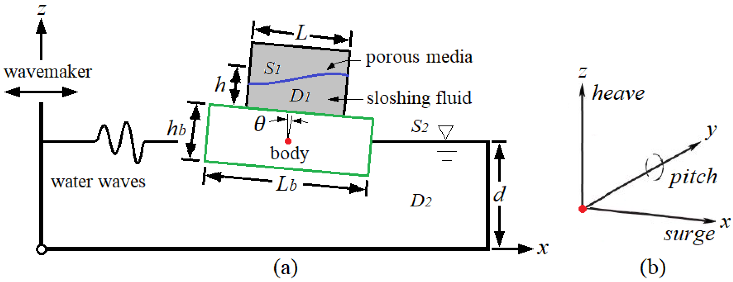
A two-dimensional rectangular water tank filled with porous media on the rectangular floating platform in waves is shown in Figure 1a. Assuming that the fluid is incompressible, inviscid, and irrotational, the continuity and momentum equations of the fluid can be expressed as:

$$\nabla ·\mathit{u}=0$$

(1)

$$\rho \left[\frac{\partial \mathit{u}}{\partial t}+\left(\mathit{u}·\nabla \right)\mathit{u}\right]=-\nabla p+\nabla p_d+\rho \mathit{g}$$

(2)

where $\rho$ is the fluid density, $\mathit{u}$ is the fluid velocity, $p$ is the pressure, $p_d$ is the pressure drop due to the porous media, and $\mathit{g}$ is the gravitational acceleration. Note that in fresh water, $\nabla p_d=0$, and nonlinearity arises only from the convective term; when the porous media is involved, the gradient of the pressure drop can be expressed by [44]:

$$\nabla p_d=-\frac{\gamma \mu }{\kappa }\left(\mathit{u}-\mathit{v}\right)-\frac{\gamma c_F\rho }{\sqrt{\kappa }}\left|\mathit{u}-\mathit{v}\right|\left(\mathit{u}-\mathit{v}\right)$$

(3)

where $\mathit{v}$ is the velocity of the porous media, $\mu$ is the dynamic viscosity of the fluid, $\gamma$ and $\kappa$ are the porosity and permeability of the porous media, respectively, and $c_F$ is a dimensionless constant determined by experiments. Note that if $\mathit{u}$ is sufficiently small, the first linear term on the right-hand side of Equation (3) dominates, while the second quadratic function becomes significant as $\mathit{u}$ increases and the drag due to solid obstacles is comparable with the surface drag due to friction. In potential flow, the fluid velocity can be expressed by the gradient of the potential function $\varphi$ as:

$$\mathit{u}=\nabla \varphi$$

(4)

Therefore, the Laplace equation should be satisfied as:

$${\nabla }^2\varphi =0$$

(5)

The kinematic boundary condition on the free surface can be expressed as:

$$\frac{D\mathit{R}}{Dt}=\mathit{u}$$

(6)

where $\mathit{R}$ is the location of a free-surface particle. For the wave channel, the dynamic boundary condition on the free surface can be expressed as:

$$\frac{\partial \varphi }{\partial t}+\frac{1}{2}{\left|\nabla \varphi \right|}^2+g\eta =0$$

(7)

where $\eta$ is the wave elevation. For the sloshing fluid, the dynamic boundary condition on the free surface can be expressed as:

$$\frac{\partial \varphi }{\partial t}+\frac{1}{2}{\left|\nabla \varphi \right|}^2+\left(\varphi -\psi \right)\left({\alpha }_1+{\alpha }_2\left|\nabla \varphi -\nabla \psi \right|\right)+g\eta =0$$

(8)

where ${\alpha }_1=\gamma \mu /\kappa \rho$ and ${\alpha }_2=c_F/\sqrt{\kappa }$ are constants related to the nature of the porous media and $\psi$ is the velocity potential of the tank. On the wetted boundaries, the impermeable condition is taken as:

$$\frac{\partial \varphi }{\partial n}=\dot{\mathit{x}}·\mathit{n}$$

(9)

where $\mathit{n}$ denotes the normal vector pointing outward to the fluid boundary and $\dot{\mathit{x}}$ is the velocity of the node on the wetted boundary. As a wave propagates along the channel, the radiation condition is applied on the outlet boundary to ensure the waves scatter to infinity as [41]:

$$\frac{\partial \varphi }{\partial n}=-\frac{1}{c}\frac{\partial \varphi }{\partial t}$$

(10)

where $c$ is the wave velocity.

Figure 1. (a) Configuration of a floating body undergoing wave excitations with a water tank, installed with porous media, attached above; (b) degree of freedom of the floating body motion.

Figure 1. (a) Configuration of a floating body undergoing wave excitations with a water tank, installed with porous media, attached above; (b) degree of freedom of the floating body motion.

2.2. Eulerian–Lagrangian Method

By applying Green’s second identity to the Laplace equation, the boundary integral equation (BIE) for the fluid boundary can be obtained as:

$$c_p{\varphi }_p={{\displaystyle \int }}_S^{}\left(\frac{\partial G}{\partial n}\varphi -G\frac{\partial \varphi }{\partial n}\right)dS$$

(11)

where $G$ is the fundamental solution with source point $p$ and $c_p$ is the resulting flux. In this paper, BIE is discretized, and the associated integrals are implemented by BEM. Therefore, Equation (11) can be rewritten in matrix form as:

$$\mathbf{A}\left\{\varphi \right\}=\mathbf{B}\left\{{\varphi }_n\right\}$$

(12)

where $\mathbf{A}$ and $\mathbf{B}$ are the kernel matrices and $\left\{\varphi \right\}$ and $\left\{{\varphi }_n\right\}$ are the vectors containing the potential and the normal velocity, respectively, at all of the boundary nodes. Equation (12) represents a mixed-type BVP with $\varphi$ given on the free surface and ${\varphi }_n$ on the wetted boundaries. The free-surface particle is tracked via a second-order Taylor series expansion, assuming a small time step, $\Delta t$, as follows:

$$\mathit{R}\left(t+\Delta t\right)=\mathit{R}\left(t\right)+\Delta t\frac{D\mathit{R}}{Dt}+\frac{\Delta t^2}{2}\frac{D^2\mathit{R}}{D{t}^2}+O\left(\Delta t^3\right)$$

(13)

$$\varphi \left(t+\Delta t\right)=\varphi \left(t\right)+\Delta t\frac{D\varphi }{Dt}+\frac{\Delta t^2}{2}\frac{D^2\varphi }{D{t}^2}+O\left(\Delta t^3\right)$$

(14)

The first-order derivative in Equation (13) is obtained by the kinematic boundary condition, while the first-order derivative in Equation (14) can be obtained by the momentum equations, i.e., Equation (7) for water waves and Equation (8) for sloshing water. The second-order derivatives of $\mathit{R}$ and $\varphi$ can be obtained as:

$$\frac{D^2{R}_i}{D{t}^2}=\frac{{\partial }^2\varphi }{\partial t\partial \mathit{x}}+\mathit{u}\nabla ·\frac{\partial \varphi }{\partial {\mathit{x}}_{\mathit{i}}}$$

(15)

$$\frac{D^2\varphi }{D{t}^2}=\mathit{u}·\frac{D\mathit{u}}{Dt}-g\frac{D\eta }{Dt}$$

(16)

A new unknown variable ${\varphi }_t=\partial \varphi /\partial t$ appears in the equations above. Since ${\varphi }_t$ also satisfies the Laplace equation, another mixed-type BVP involving ${\varphi }_t$ and ${\varphi }_{tn}$ arises and needs to be solved. The Dirichlet condition on the free surface is given by:

$${\varphi }_t=\frac{D\varphi }{Dt}-{\left|\nabla \varphi \right|}^2$$

(17)

The Neumann condition on the wetted boundaries is given by:

$${\varphi }_{tn}=\ddot{\mathit{x}}·\mathit{n}-\left(\mathit{u}·\nabla \right){\varphi }_n,$$

(18)

while the Neumann condition on the radiation boundary is given by:

$${\varphi }_{tn}=c\frac{{\partial }^2\varphi }{\partial s^2}$$

(19)

where $\ddot{\mathit{x}}$ is the acceleration of the node on the wetted boundary and $s$ denotes the tangential direction of the boundary. Fortunately, the domain geometry remains unchanged at the current time step, so the matrices $\mathbf{A}$ and $\mathbf{B}$ in Equation (12) can be reused.

2.3. Floating Body Dynamics and FSI Coupling

In this paper, the floating body motion has three degrees of freedom, namely it is free to surge (horizontal movement along the x direction), heave (vertical movement along the z direction), and pitch (angular movement about the y-axis), as shown in Figure 1b. Therefore, the equations of translational and angular motions can be expressed as:

$$M_b{\ddot{\mathit{x}}}_G=\mathit{F}+M_b\mathit{g}$$

(20)

$$I_G{\ddot{\mathit{\theta }}}_G=\mathit{M}$$

(21)

where ${\ddot{\mathit{x}}}_G$ and ${\ddot{\mathit{\theta }}}_G$ are the translational and angular acceleration of the body center, respectively, while $M_b$ and $I_G$ are the mass and moment of inertia of the body, respectively. The resultant force $\mathit{F}$ and overturning moment $\mathit{M}$ arising from the sloshing fluid and waves can be expressed as:

$$\mathit{F}={{\displaystyle \int }}_{S_{w1}+S_{w2}}^{}p\mathit{n} dS$$

(22)

$$\mathit{M}={{\displaystyle \int }}_{S_{w1}+S_{w2}}^{}p\left(\mathit{r}\times \mathit{n}\right) dS$$

(23)

where $S_{w1}$ and $S_{w2}$ are the wetted boundaries of the floating body’s contact with the sloshing water and waves, respectively, and $\mathit{r}$ is the position vector of a fluid particle with respect to the body center. The pressure can be obtained by the Bernoulli equation as:

$$p=-\rho \left(\frac{\partial \varphi }{\partial t}+\frac{1}{2}{\left|\nabla \varphi \right|}^2+g\eta \right)$$

(24)

To solve the motion equations, the Newmark method based on the constant average acceleration assumption is employed as:

$${\ddot{\mathit{x}}}_{G,k+1}=\frac{{\mathit{F}}_{k+1}}{M_b}$$

(25)

$${\dot{\mathit{x}}}_{G,k+1}={\dot{\mathit{x}}}_{G,k}+0.5\Delta t\left({\ddot{\mathit{x}}}_{G,k}+{\ddot{\mathit{x}}}_{G,k+1}\right)$$

(26)

$${\mathit{x}}_{G,k+1}={\mathit{x}}_{G,k}+\Delta t{\dot{\mathit{x}}}_{G,k}+0.25\Delta t^2\left({\ddot{\mathit{x}}}_{G,k}+{\ddot{\mathit{x}}}_{G,k+1}\right)$$

(27)

where $k$ is the time step. Note that the above equations are available for solving the translational motion, while the angular motion can be solved by switching the force and mass in Equation (25) to the overturning moment and moment of inertia, respectively. This scheme is unconditionally stable and it does not need a sub-step. However, the resultant force is not known a priori because, to solve the fluid field, the body kinematics used in Equations (9) and (18) should be given but they depend on the body motion as:

$$\dot{\mathit{x}}=\left({\dot{\mathit{x}}}_G+{\dot{\mathit{\theta }}}_G\times \mathit{r}\right)·\mathit{n}$$

(28)

$$\ddot{\mathit{x}}=\left[{\ddot{\mathit{x}}}_G+{\ddot{\mathit{\theta }}}_G\times \mathit{r}+{\dot{\mathit{\theta }}}_G\times \left({\dot{\mathit{\theta }}}_G\times \mathit{r}\right)\right]·\mathit{n}$$

(29)

Therefore, an iterative algorithm, illustrated in Algorithm 1, is used to ensure equilibrium between the body motion and fluid reaction.

Algorithm 1: An iterative algorithm for FSI by EL method.

do k > 0  Start iterative step with the solution at kth time step as an initial guess  $ϵ=abs\left({\ddot{\mathit{x}}}_{G,k,i}-{\ddot{\mathit{x}}}_{G,k,i-1}\right)$  do while $ϵ>{ϵ}_{tolerance}$  Solve ${\varphi }_i$ and ${\varphi }_{n,i}$ (the first BVP)  Solve ${\varphi }_{t,i}$ and ${\varphi }_{tn,i}$ (the second BVP)  Calculate pressure along wetted boundaries  Calculate force and moment act on the floating body  Define predictor of force and moment: ${\mathit{F}}^{*}={\mathit{F}}_{k,i}+\omega \left({\mathit{F}}_{i-1}^{*}-{\mathit{F}}_{k,i}\right)$  Solve rigid-body motion (Newmark method)  Update free surface and body boundary $S_{k,i+1}$ and ${\varphi }_{k,i+1}$  end do  ${\mathit{x}}_{k+1}={\mathit{x}}_{k,i+1}$  ${\dot{\mathit{x}}}_{k+1}={\dot{\mathit{x}}}_{k,i+1}$  ${\ddot{\mathit{x}}}_{k+1}={\ddot{\mathit{x}}}_{k,i+1}$  ${\varphi }_{k+1}={\varphi }_{k,i+1}$  $S_{k+1}=S_{k,i+1}$ end do

2.4. Equivalent Mechanical Model

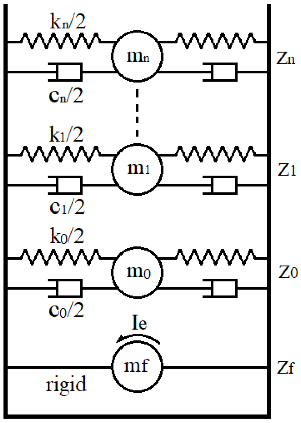
In addition to the EL method, the mechanical model can be useful to solve the sloshing problem in porous media by means of a series of motion equations. For the rectangular tank, the mechanical model consists of a fixed mass $m_f$ located at the height $z_f$, and infinite mass-dashpot-spring systems (denoted by $m_n$, $c_n$, and $k_n$) located at the heights $z_n$ as shown in Figure 2. The equivalent masses, stiffness, damping ratios, and location heights can be expressed as [24]:

$$m_n=\frac{8\gamma \rho B}{a_n^{3}L}tanh a_{n}h$$

(30)

$$k_n=m_n{\omega }_n^2=\frac{8\gamma \rho gB}{a_n^{2}L}tan{h}^2{a}_{n}h$$

(31)

$${\xi }_n=\frac{{\alpha }_1}{2{\omega }_n}=\frac{\gamma \mu }{2\kappa \rho {\omega }_n}=\frac{\gamma \mu }{2\kappa \rho }\sqrt{\frac{coth{a}_{n}h}{a_{n}g}}$$

(32)

$$z_n=h+\frac{2}{a_{n}sinh{a}_{n}h}-\frac{1}{a_{n}tanh{a}_{n}h}$$

(33)

$$m_f=m_w-{{\displaystyle \sum }}_{n=0}^{\infty }{m}_n=\gamma \rho BLh\left[1-{\displaystyle \sum }_{n=0}^{\infty }\frac{8}{a_n^3{L}^{2}h}tanh{a}_{n}h\right]$$

(34)

$$z_f=\frac{1}{m_f}\left[\gamma \rho B\left(\frac{L{h}^2}{2}+\frac{L^3}{12}\right)-{\displaystyle \sum }_{n=0}^{\infty }{m}_n{z}_n\right]$$

(35)

where $a_n=\left(2n+1\right)\pi /L$, $n=0,1,2\cdots$, $m_w=\gamma \rho BLh$ denotes the total water mass in the tank, and $B$ is the tank width. The above equivalent parameters are obtained when the tank is subject to horizontal excitations. However, it is not sufficient to describe the angular motion studied in this paper. The moment of inertia should be appended to satisfy dynamic equilibrium. As the tank is subjected to a harmonic pitch motion, its angular displacement is expressed by:

$$\theta \left(t\right)={\theta }_{0}sin\omega t$$

(36)

where ${\theta }_0$ is the amplitude of angular displacement. The velocity potential on the walls and bottom should satisfy the impermeable boundary condition as:

$$\frac{\partial \varphi }{\partial x}={\theta }_0\omega zcos\omega t, \mathrm{on} \mathrm{wetted} \mathrm{walls}$$

(37)

$$\frac{\partial \varphi }{\partial z}=-{\theta }_0\omega xcos\omega t, \mathrm{on} \mathrm{bottom}$$

(38)

Hence the velocity potential can be expressed as:

$$\begin{array}{cc}\hfill \varphi ={\theta }_0\omega cos\omega t& {\displaystyle {\displaystyle \sum }_{n=0}^{\infty }}4{\left(-1\right)}^n[\frac{sin{b}_n\left(z-\frac{h}{2}\right)}{b_n^{3}h}\frac{sinh{b}_{n}x}{cosh{b}_n\frac{L}{2}}+\frac{sin{a}_{n}x}{a_n^{3}L}\frac{cosh{a}_n\left(z-h\right)}{sinh{a}_{n}h}]\hfill \\ & +{\theta }_0\omega {\displaystyle {\displaystyle \sum }_{n=0}^{\infty }}\left(D_{1n}cos\omega t+D_{2n}sin\omega t\right)sin{a}_{n}x cosh{a}_{n}z\hfill \end{array}$$

(39)

where $b_n=\left(2n+1\right)\pi /h$. On the free surface, the linear kinematic and dynamic boundary conditions are combined and applied at $z=h$ as:

$$\frac{{\partial }^2\varphi }{\partial t^2}+{\alpha }_1\left(\frac{\partial \varphi }{\partial t}-\frac{\partial \psi }{\partial t}\right)+g\frac{\partial \varphi }{\partial z}=0$$

(40)

Substituting Equation (39) into Equation (40), the coefficients $D_{1n}$ and $D_{2n}$ can be solved as:

$$D_{1n}=\frac{-p_n}{p_n^2+q_n^2}\frac{4{\omega }^2}{sin{a}_{n}xcosh{a}_{n}h}\left[\frac{sinh{b}_{n}x}{b_n^{3}hcosh{b}_n\frac{L}{2}}+\frac{{\left(-1\right)}^{n}sin{a}_{n}x}{a_n^{3}Lsinh{a}_{n}h}\right]$$

(41)

$$D_{2n}=\frac{q_n}{p_n^2+q_n^2}\frac{4{\omega }^2}{sin{a}_{n}xcosh{a}_{n}h}\left[\frac{sinh{b}_{n}x}{b_n^{3}hcosh{b}_n\frac{L}{2}}+\frac{{\left(-1\right)}^{n}sin{a}_{n}x}{a_n^{3}Lsinh{a}_{n}h}\right]$$

(42)

where $p_n={\omega }^2-g{a}_{n}tanh{a}_{n}h$ and $q_n=\gamma {\alpha }_1\omega$. The overturning moment due to the sloshing fluid can be obtained by integrating the pressure along the wetted boundary as:

$$M_o=\gamma \rho {{\displaystyle \int }}_0^h{{\displaystyle \int }}_0^B\left({\frac{\partial \varphi }{\partial t}|}_{x=\frac{L}{2}}-{\frac{\partial \varphi }{\partial t}|}_{x=\frac{-L}{2}}\right)zdydz+\gamma \rho {{\displaystyle \int }}_{-L/2}^{L/2}{{\displaystyle \int }}_0^B{\frac{\partial \varphi }{\partial t}|}_{z=0}xdydx$$

$$\begin{array}{c}=-\gamma \rho B{\theta }_0{\omega }^{2}sin\omega t{\displaystyle {\displaystyle \sum }_{n=0}^{\infty }}8\left[\frac{3sinh{b}_n\frac{L}{2}-b_n\frac{L}{2}cosh{b}_n\frac{L}{2}}{b_n^{5}hcosh{b}_n\frac{L}{2}}+\frac{2cosh{a}_{n}h-1}{a_n^{5}Lsinh{a}_{n}h}\right]\hfill \\ +\gamma \rho B{\theta }_0{\omega }^2{\displaystyle {\displaystyle \sum }_{n=0}^{\infty }}\frac{8{\omega }^2\left(p_{n}sin\omega t+q_{n}cos\omega t\right)}{\left(p_n^2+q_n^2\right)cosh{a}_{n}h}[\frac{b_n\frac{L}{2}cosh{b}_n\frac{L}{2}-sinh{b}_n\frac{L}{2}}{b_n^{5}hcosh{b}_n\frac{L}{2}}\hfill \\ +\frac{a_{n}hsinh{a}_{n}h-cosh{a}_{n}h+2}{a_n^{5}Lsinh{a}_{n}h}+\frac{\left(a_{n}hsinh{a}_{n}h-cosh{a}_{n}h+1\right)tanh{b}_n\frac{L}{2}}{a_n^2{b}_n^{3}h}]\hfill \end{array}$$

(43)

Based on the dynamic equivalent, the mechanical model should give the same overturning moment under the same circumstances. Therefore, the motion equation of the mechanical system can be written as:

$$m_n{\ddot{x}}_n+c_n{\dot{x}}_n+k_n{x}_n=m_n{z}_n{\theta }_0{\omega }^{2}sin\omega t$$

(44)

where $x_n$ is the equivalent displacement of the moving mass relative to the ground. The overturning moment can be obtained as:

$${\overline{M}}_o=I_e\ddot{\theta }+m_f{z}_f{z}_f\ddot{\theta }+{\displaystyle \sum }_{n=0}^{\infty }{m}_n{z}_n{z}_n\ddot{\theta }+{\displaystyle \sum }_{n=0}^{\infty }{m}_n{z}_n{\ddot{x}}_n$$

$$=\left(I_e+m_f{z}_f^2+{\displaystyle \sum }_{n=0}^{\infty }{m}_n{z}_n^2\right)\ddot{\theta }+{\displaystyle \sum }_{n=0}^{\infty }{m}_n{z}_n{\ddot{x}}_n$$

(45)

Using the same technique described in reference [24] to equalize the overturning moments due to rigid-body motion (regardless of the oscillatory component), i.e., the first term on the right-hand side of Equations (43) and (45), the moment of inertia $I_e$ can be obtained as:

$$I_e=8\gamma \rho B{\displaystyle \sum }_{n=0}^{\infty }\left(\frac{3sinh{b}_n\frac{L}{2}-b_n\frac{L}{2}cosh{b}_n\frac{L}{2}}{b_n^{5}hcosh{b}_n\frac{L}{2}}+\frac{2cosh{a}_{n}h-1}{a_n^{5}Lsinh{a}_{n}h}-m_n{z}_n^2\right)-m_f{z}_f^2$$

(46)

Figure 2. The schematic diagram of the equivalent mechanical model of a water tank filled with porous media.

Figure 2. The schematic diagram of the equivalent mechanical model of a water tank filled with porous media.

When the mechanical model is applied to the floating body, its motion equation can be expressed as:

$$m_n{\ddot{x}}_n+c_n{\dot{x}}_n+k_n{x}_n=-m_n{\ddot{x}}_G+m_n{z}_n{\ddot{\theta }}_G$$

(47)

Therefore, Equation (25) for the surge motion of the floating body can be modified by:

$$M_b{\ddot{x}}_G={{\displaystyle \int }}_{S_{w2}}^{}p{n}_{x}dS+m_f{z}_f{\ddot{\theta }}_G+{\displaystyle \sum }_{n=0}^{\infty }\left(c_n{\dot{x}}_n+k_n{x}_n+m_n{z}_n{\ddot{\theta }}_G\right)$$

(48)

For the heave motion, the mechanical model assumes no masses move vertically relative to the tank, so the entire system will be regarded as a dead load to the floating body. Therefore, the equilibrium equation can be simplified as:

$$M_b{\ddot{z}}_G={{\displaystyle \int }}_{S_{w2}}^{}p{n}_{z}dS-m_{w}g$$

(49)

For the pitch motion, the movement of the equivalent masses will produce an external moment on the floating body; therefore, the equilibrium equation can be modified by:

$$I_b{\ddot{\theta }}_G={{\displaystyle \int }}_{S_{w2}}^{}p\left(\mathit{r}\times \mathit{n}\right) dS-\left(I_e+m_f{z}_f^2\right){\ddot{\theta }}_G-{\displaystyle \sum }_{n=0}^{\infty }\left(c_n{\dot{x}}_n+k_n{x}_n+m_n{z}_n{\ddot{\theta }}_G\right)z_n$$

(50)

During the computation of Equations (48)–(50), the resultants from the sloshing behavior can be obtained once Equation (47) is solved. Since the sloshing computation does not go through the EL method, the numerical simulation is very efficient and inexpensive.

3. Characteristics Analysis for Floating Body

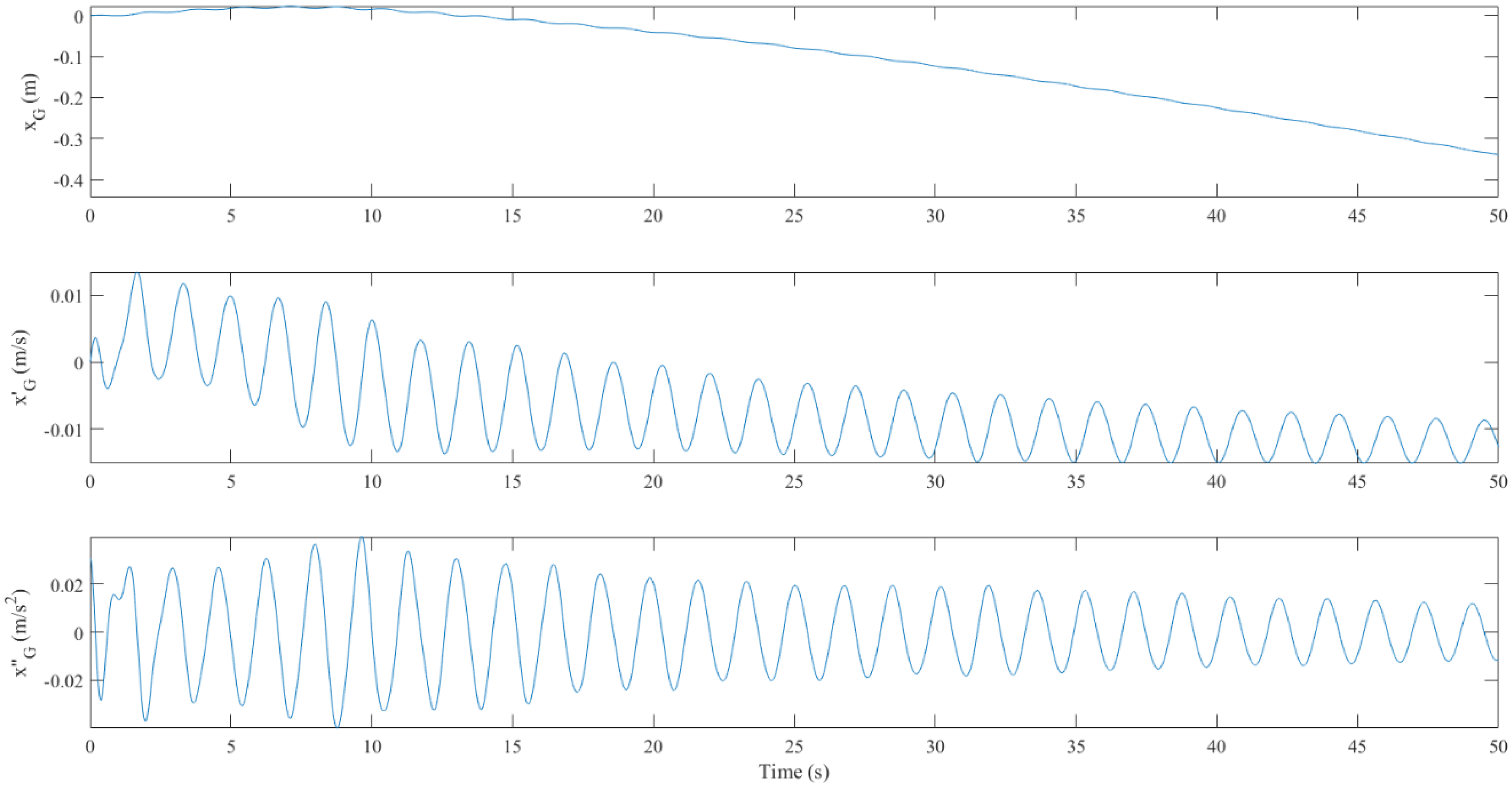
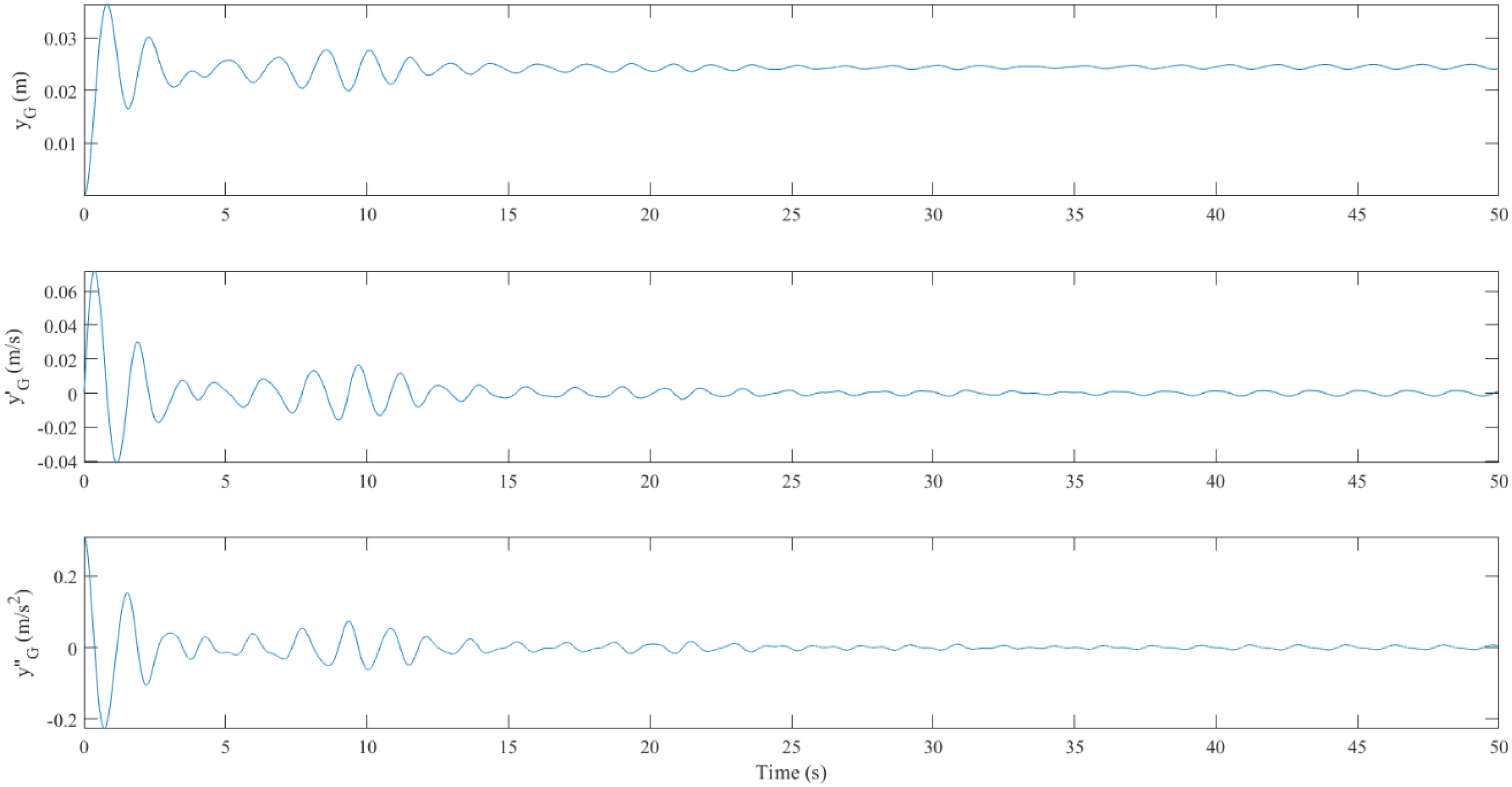
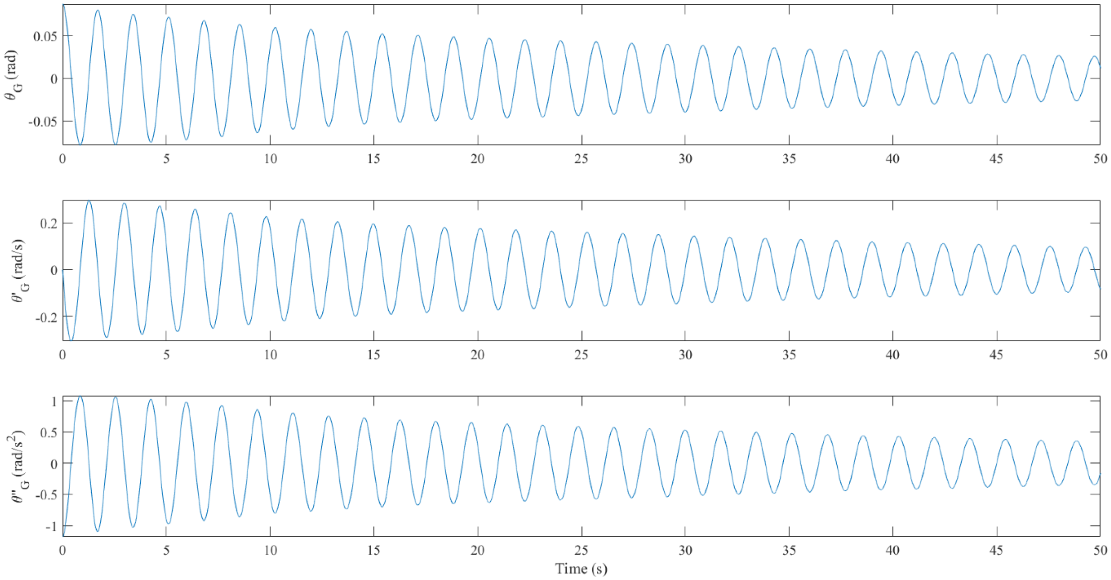
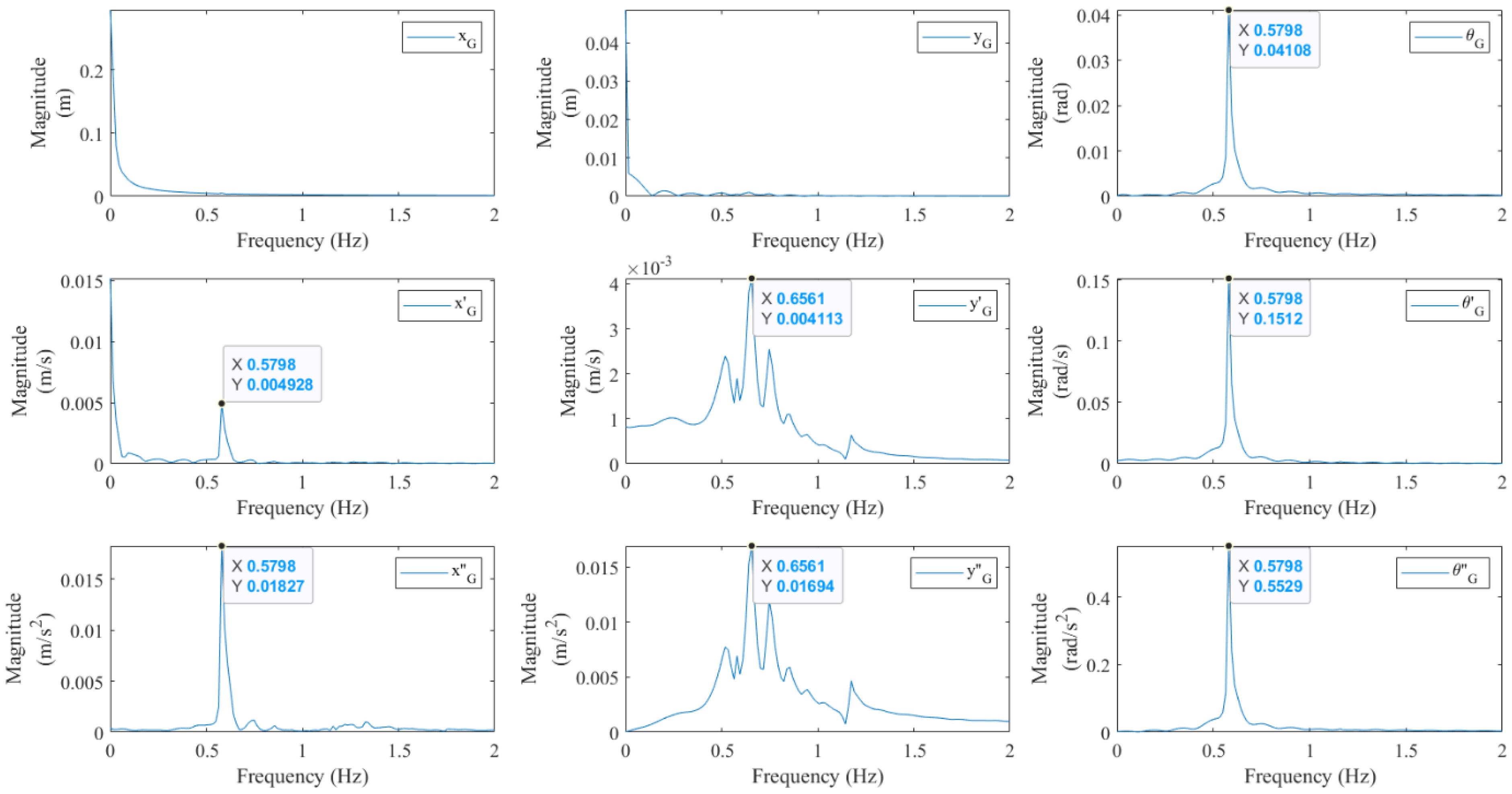
The dynamic characteristics of a rectangular floating body were examined through a free-vibration test. The channel length = 10 m and water depth = 2 m. The rectangular floating platform had its length = 1 m, height = 0.5 m, and density = 450 kg/m³, meaning the body mass = 225 kg and moment of inertia = 23.44 kg-m². Its center of gravity was placed at x = 5m and y = 2m, which was at the same height as the still water surface. The initial inclined angle was 5°. A total of 1714 two-node linear elements were distributed on the boundary of the water in the channel. The time interval was 0.001 s. As no incident waves were applied, the free vibration of the surge, heave, and pitch motions of the body are shown in Figure 3, Figure 4 and Figure 5, respectively. The corresponding response spectra are shown in Figure 6. In Figure 3, the horizontal drift was small, even without the mooring constraint. Since the horizontal force came from the pressure difference between the left and right sides of the body, which was in sync with the pitch motion, the surge velocity and acceleration had the same oscillatory frequency of 0.58 Hz as the pitch motion, as shown in Figure 6. The heaving frequency = 0.66 Hz. Compared to the solution of a hanging spring model, regardless of the added mass effect (0.74 Hz), the numerical result was reasonable for a partially immersed body. In Figure 4, the heave motion decayed because the storing potential energy was passed to ambient waves and then carried away through the radiation condition. It eventually reached the static displacement of 0.0245 m. For the pitch motion, slight decay was observed. This has been explained in the past article [30]; the amplitude of the pitch motion could be over-predicted in potential flow since the wave damping was neglected. However, the pitching frequency = 0.58 Hz would not be affected. All the body motions were quite linear.

4. Results and Discussion

The first example compares the nonlinear EL method and the linear mechanical model. The accuracy of the mechanical model on pitch-motion simulation is verified. The second example presents the numerical results of a water tank with and without porous media to accentuate the effect of porous media on the wave-induced sloshing phenomenon. The third example shows the benefit of this research in vibration control for offshore structures and sloshing mitigation for LNG vessels via frequency response analysis.

4.1. Sloshing in a Tank Filled with Porous Media: EL Method vs. Mechanical Model

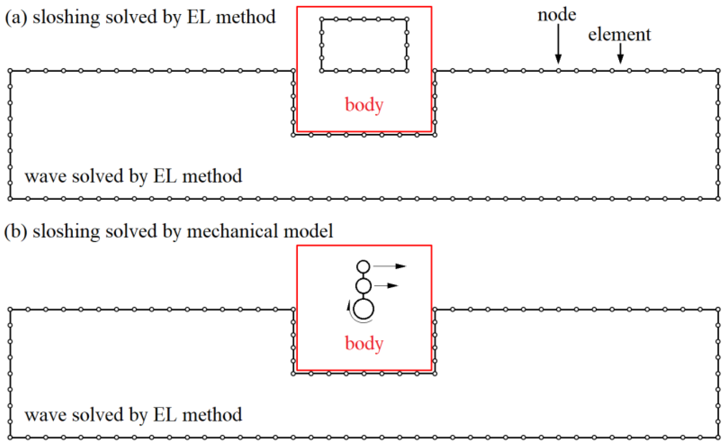
In this example, the configuration of a rectangular body in the wave channel is the same as described in Section 3. The piston-type wavemaker was set on the left side of the channel to generate harmonic waves that propagated along the x direction to the right side. The wave frequency was 0.58 Hz, which was resonant with the floating body. Two cases were tested. The large wave had its wave height = 0.05 m, so the demand stroke of the wavemaker was 2.64 cm, while the small wave had its wave height = 0.03 m, so the demand stroke of the wavemaker was 1.58 cm [45]. The water tank was installed in a way in which the bottom was aligned with the centerline of the floating body. The tank length was 0.64 m and the water depth was 0.047 m, hence the fundamental sloshing frequency was 0.53 Hz. The masses of the tank and porous media were neglected. The porosity of the porous media = 0.96. Assume the first modal damping ratio was 18.4%, which results in ${\alpha }_1$ = 1.28 s⁻¹ and ${\alpha }_2$ = 5.0 m⁻¹ being used in the EL method [26]. A total of 80 two-node linear elements were distributed on the boundary of the sloshing fluid. When the mechanical model was applied, both the single-degree-of-freedom (SDOF) (namely, only the fundamental sloshing mode was considered) and five-degree-of-freedom (5-DOF) (namely, the first five sloshing modes were considered) systems were tested. The numerical configurations for the EL method and mechanical model are shown in Figure 7.

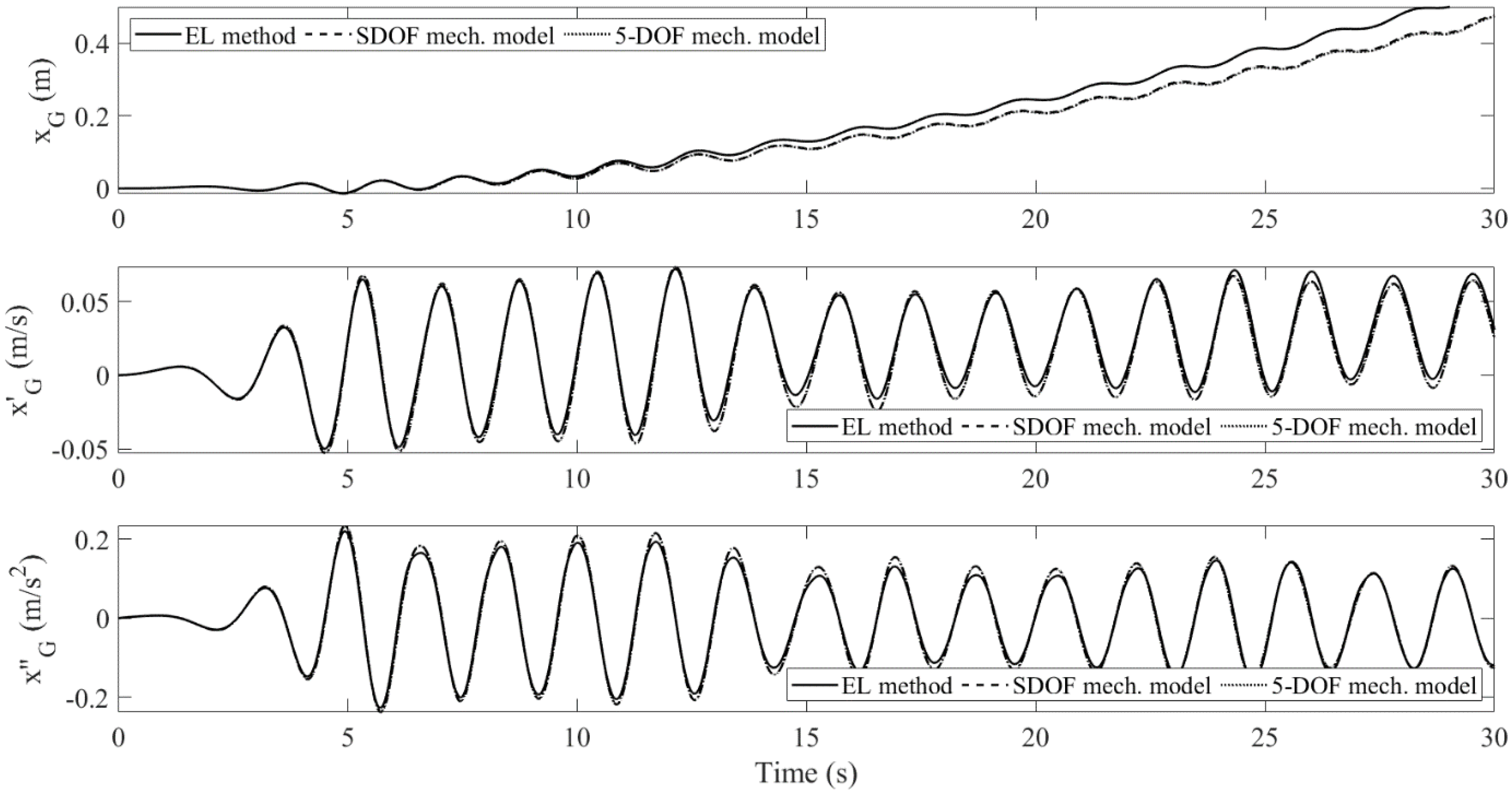
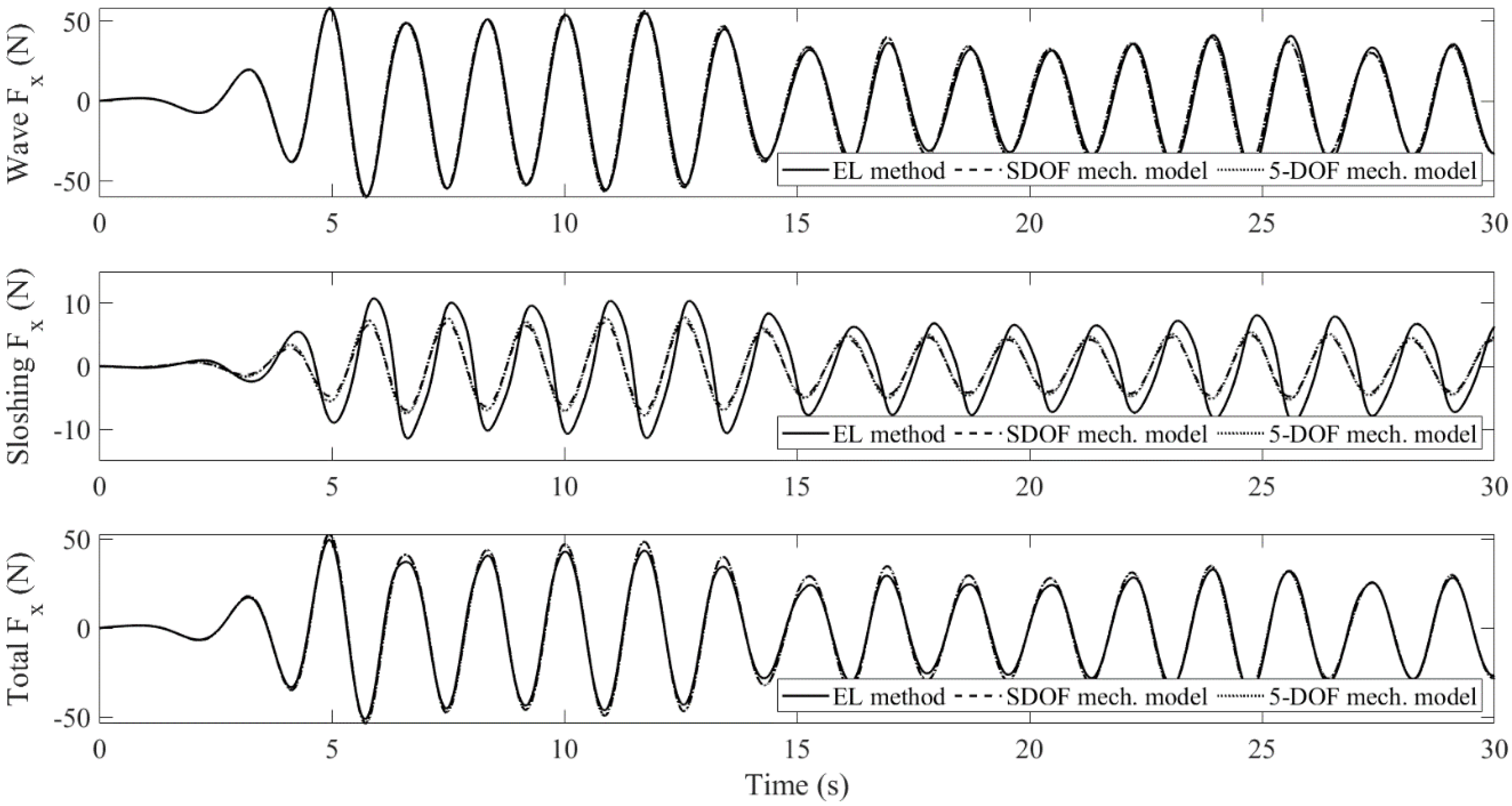
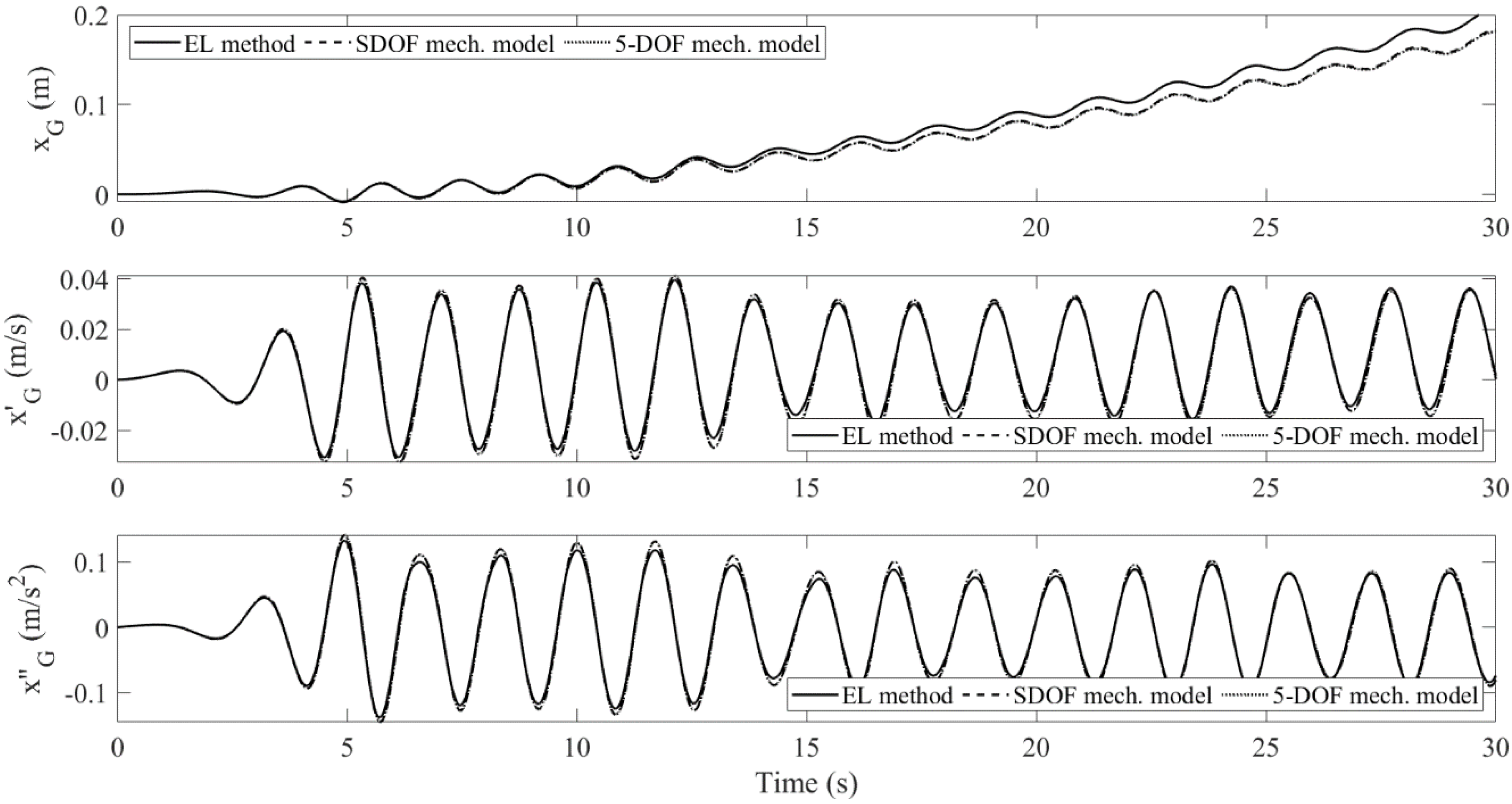
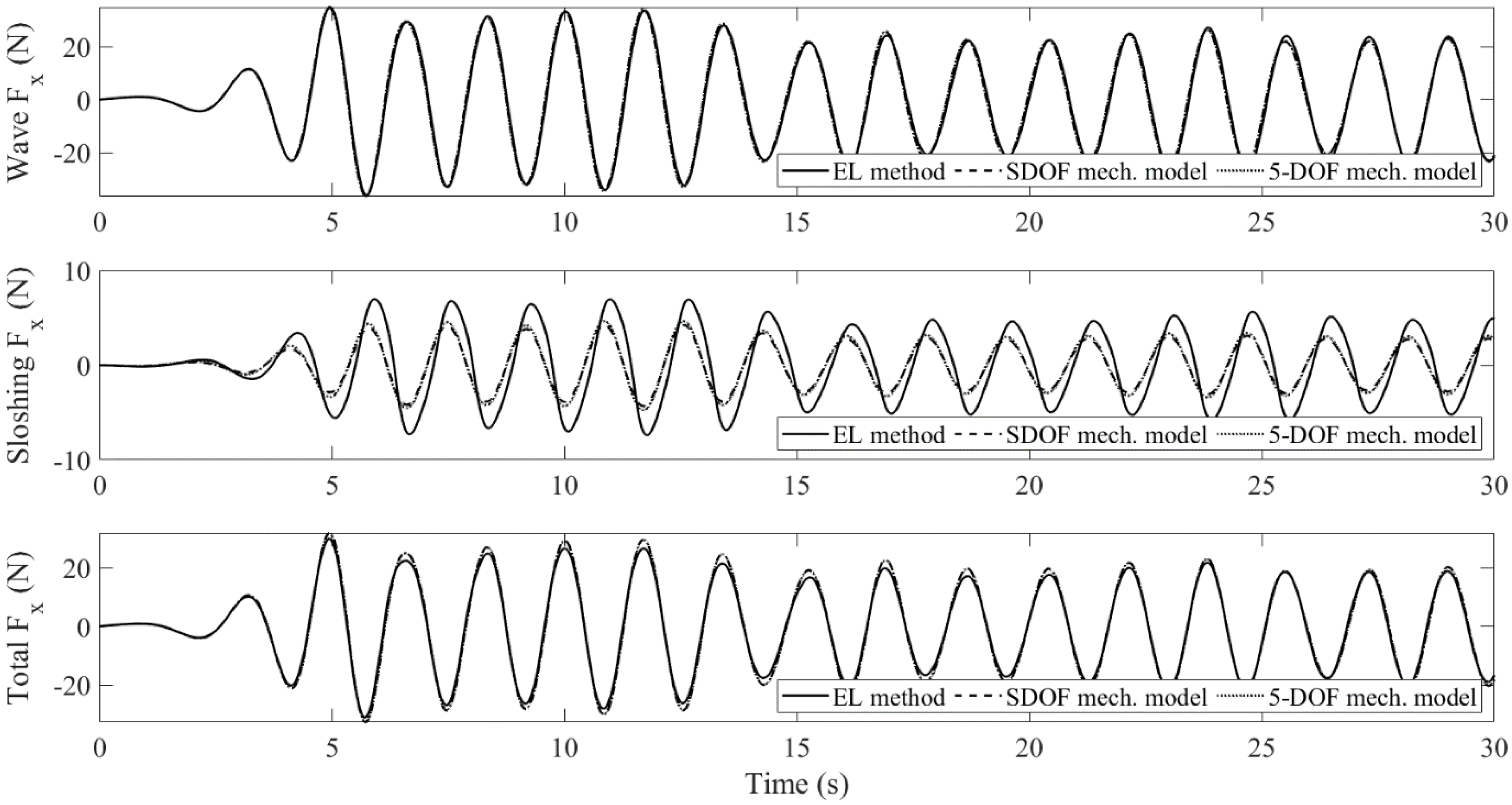
The surge motion responses of the floating body undergoing large wave excitation are shown in Figure 8. The body drifted along the x direction due to the continuous incoming waves. The numerical displacements were slightly different but the accelerations and velocities were very close. Since the dynamic responses depended on the external forces, their correlation will be explained via the horizontal forces as shown in Figure 9. The sloshing force cancels out the wave load due to phase cancellation. The EL method had a larger sloshing reaction, hence a smaller total force and a smaller acceleration were obtained. It is noticeable that in past experiments [25], the mechanical model overestimated the sloshing force. However, in our case, the external excitations to the water tank were different as the coupling effect was involved. Therefore, one may not always expect an over-predicted value from the mechanical model.

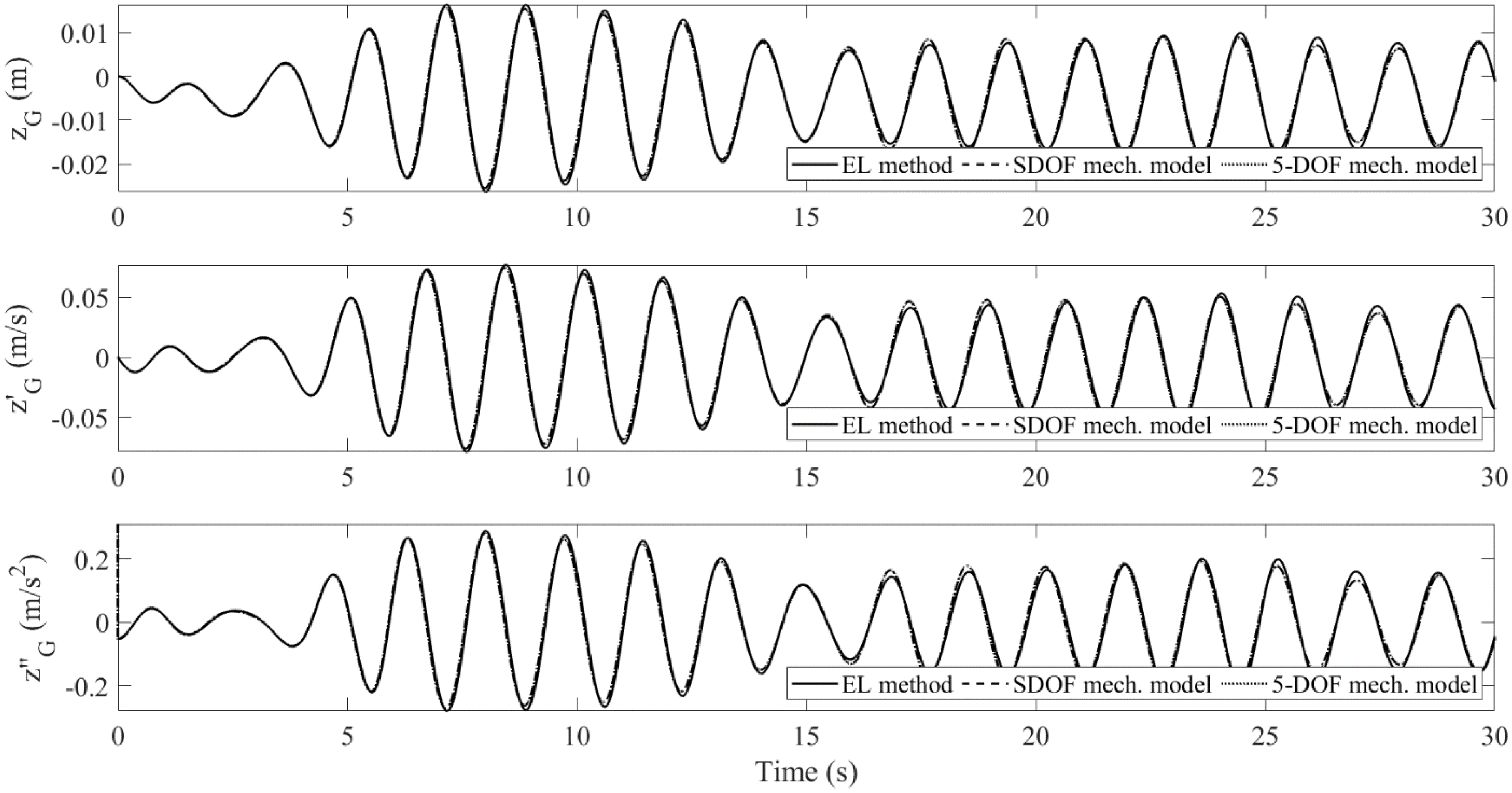
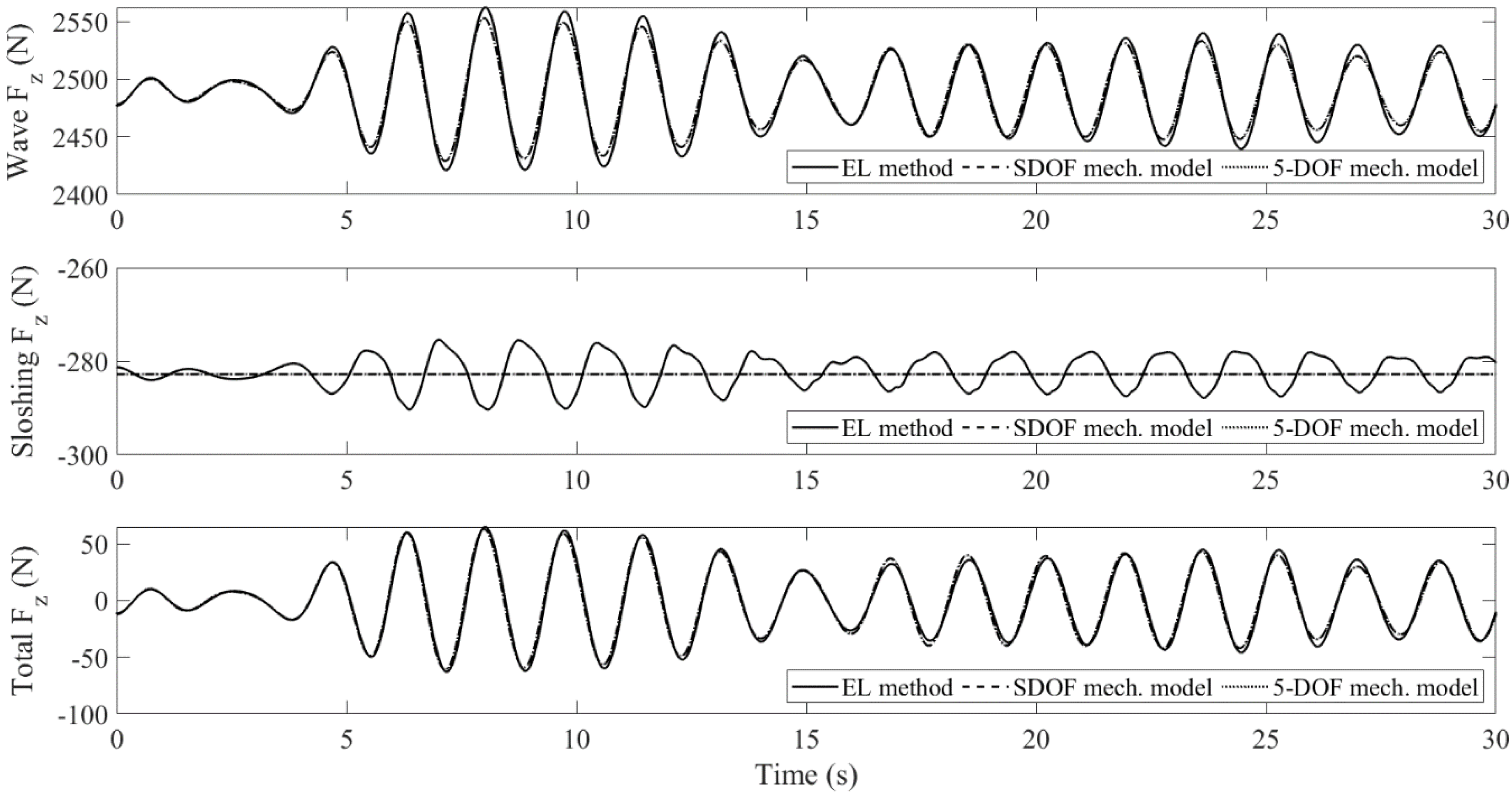
The heave motion responses of the floating body and the vertical resultant forces to the body are shown in Figure 10 and Figure 11, respectively. The mean value of the steady-state displacement was −0.0043 m, which was the same as the static displacement. The responses by both methods were identical except for the sloshing force. The mechanical model assumes the vertical sloshing force as a dead load, while the EL method takes the dynamic force due to the momentum change and convective acceleration into account. However, this effect was not significant in the vertical direction. It only caused a 3% (10 N) deviation from the dead load. Therefore, the heave response remained the same.

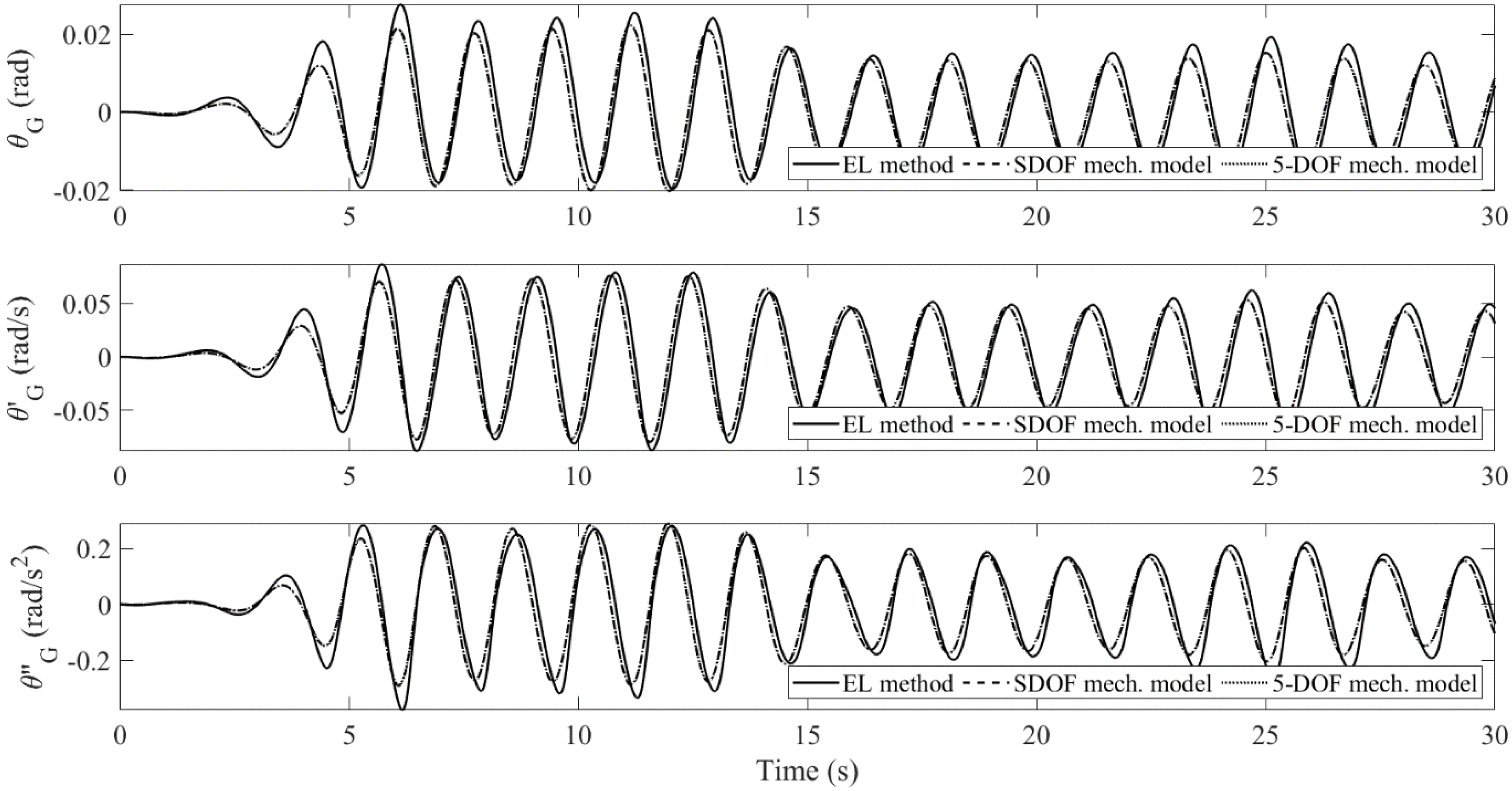
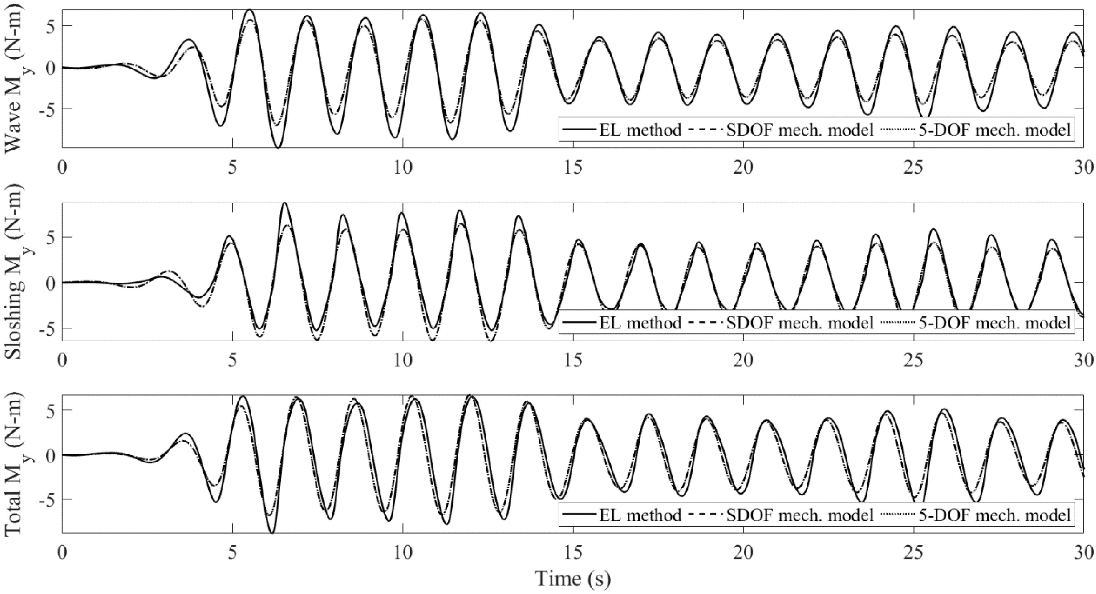
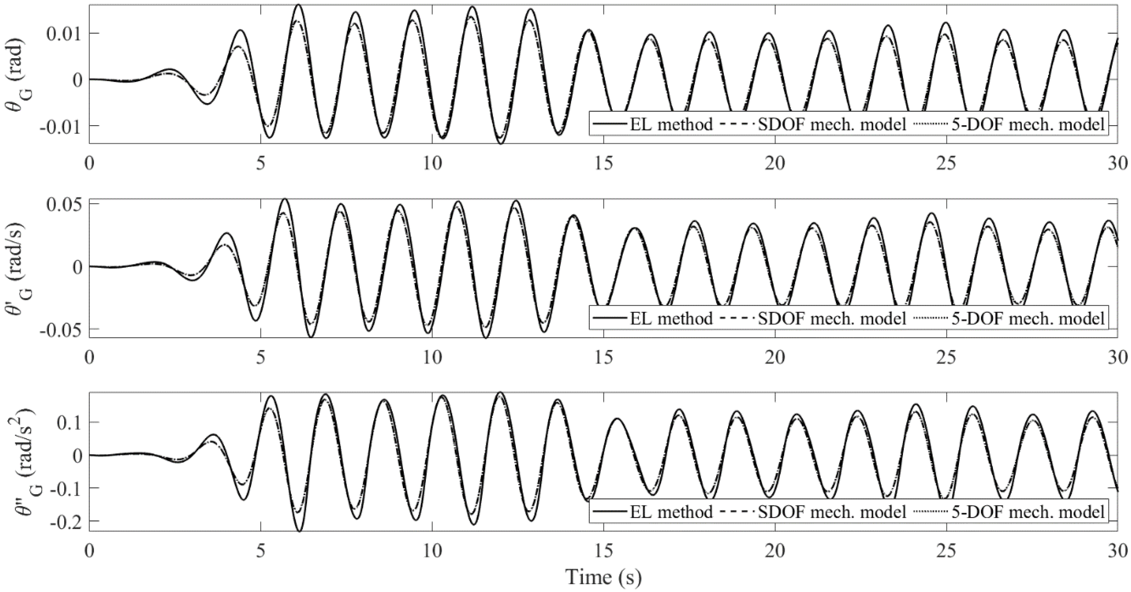
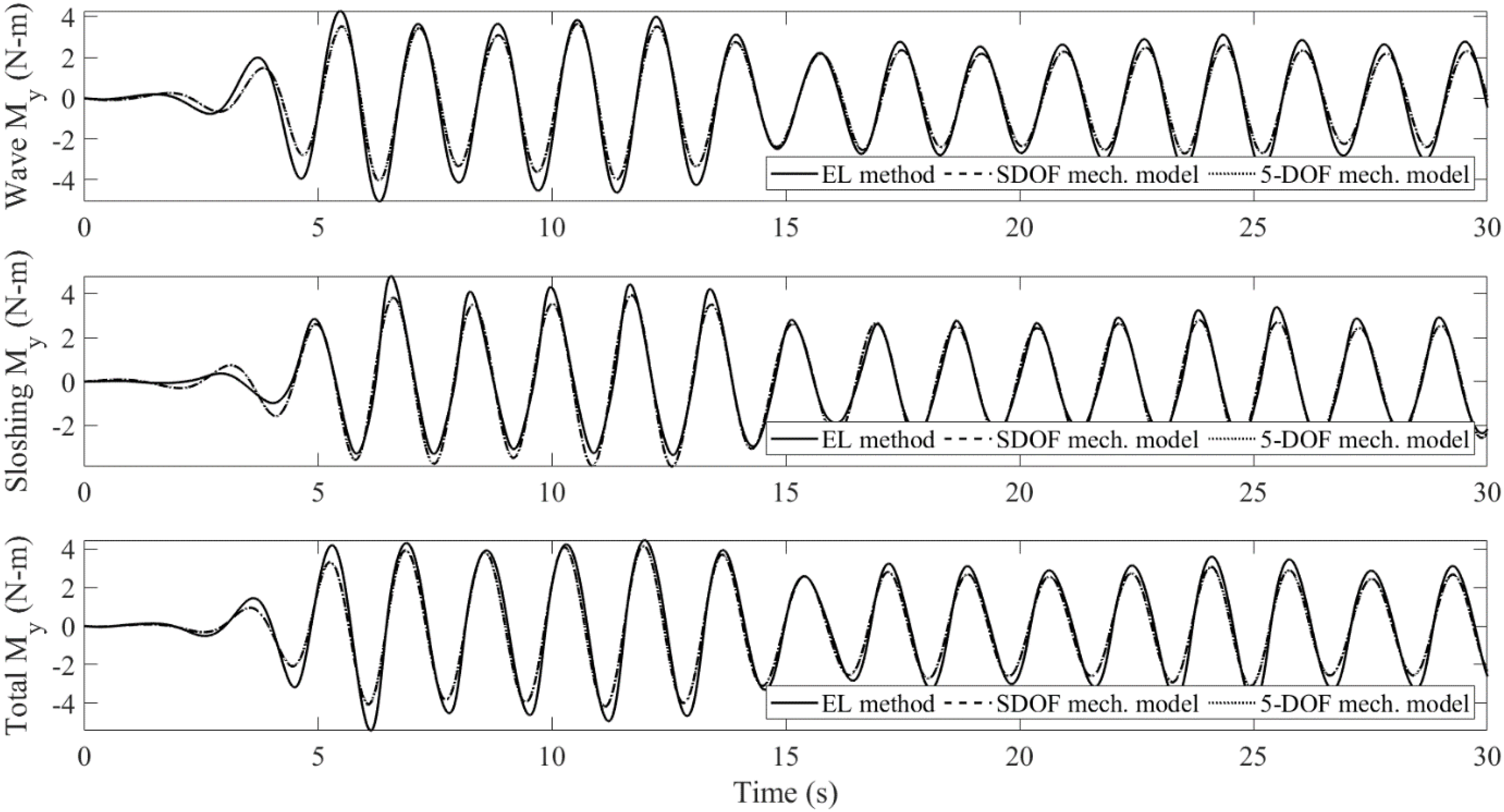
The pitch motion responses of the floating body and the overturning moments to the body are shown in Figure 12 and Figure 13, respectively. The sloshing overturning moment by the EL method was nonlinear, while that by the mechanical model was linear. It is important to take the nonlinear effect into account since it changed the pitch amplitudes of the body in this example. The phase cancellation appeared. Since the sloshing-induced moment was comparable to the wave-induced moment, the moment cancellation was fairly strong. The body responses and sloshing reactions by the SDOF and five-DOF mechanical systems were identical for the surge, heave, and pitch motions. This shows that the fundamental mode dominated and the high-mode sloshing responses were too small to affect the FSI behavior. It justifies the design strategies for the liquid dampers that only emphasized the first modal response [22].

When the small wave excitation was applied, the body motions and the resultant forces along three directions are shown in Figure 14, Figure 15, Figure 16, Figure 17, Figure 18 and Figure 19. The overall trends were similar to what was observed for the large-wave cases. However, the smaller wave loadings caused a smaller body vibration, hence lowering the nonlinear effect in the sloshing reactions. The mechanical model captured the pitch motion more easily. Similarly, the resultant forces and body dynamics by the SDOF and five-DOF mechanical systems highly coincided.

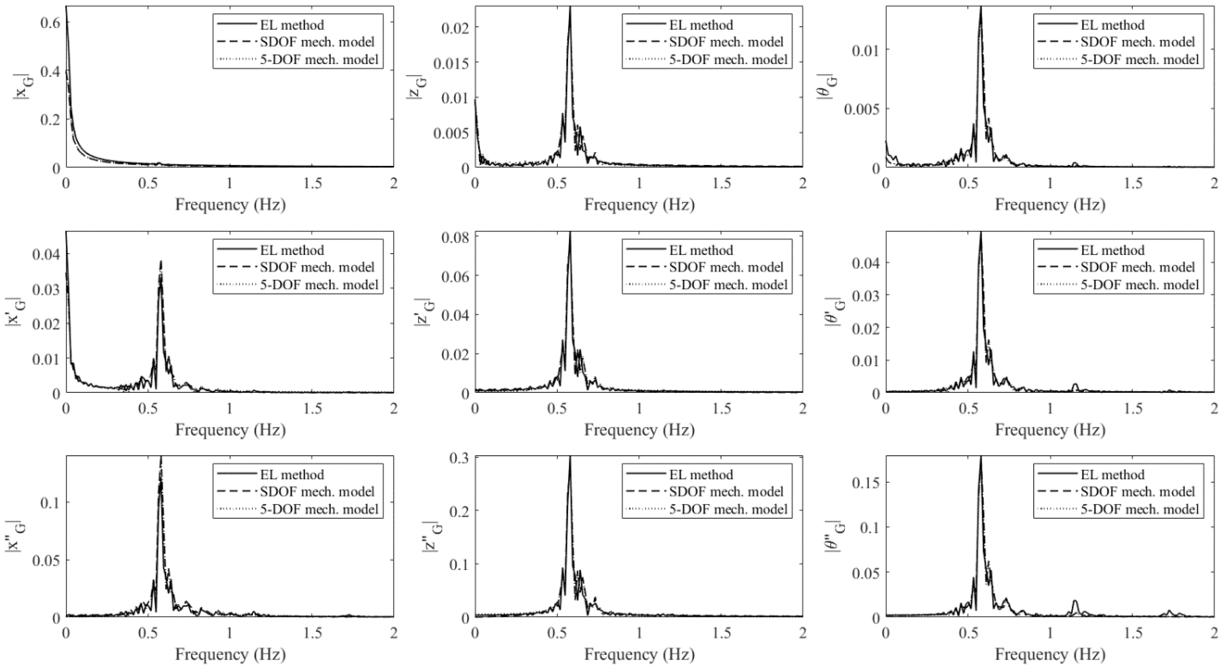
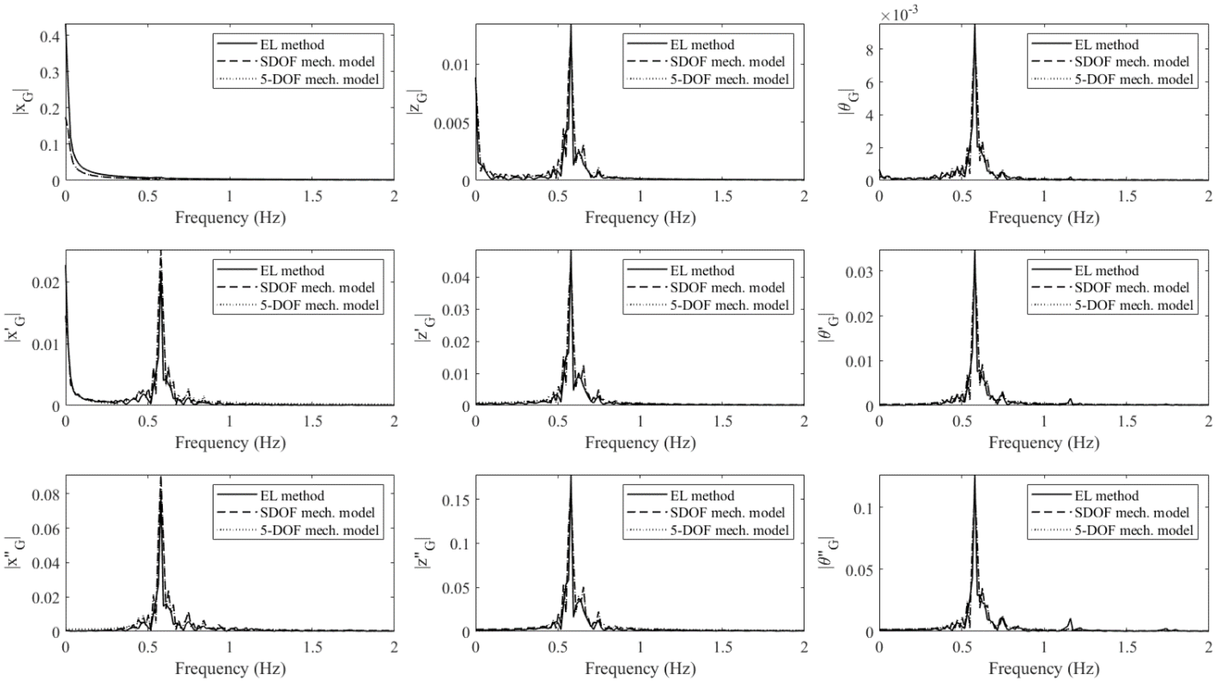
The response spectra of the body motions for the large- and small-wave cases are shown in Figure 20 and Figure 21, respectively. The spectra by both methods are very similar, hence the mechanical model ensured the consistency of the dynamic characteristics of the sloshing behavior. The response spectra by the SDOF and 5-DOF mechanical systems are also identical, so the importance of the first modal response was validated in the frequency domain. Both methods showed one peak at the resonant frequencies for each motion, but the EL method observed another local peak at the double frequency (1.16 Hz) of the angular response spectra. This means the nonlinear effect due to the convective term appeared. No peak at the double frequency was observed by the mechanical model because the nonlinear effect was neglected. However, this phenomenon was not obvious in the small-wave case as shown in Figure 21. Besides, the response spectra of the surge and heave motions had no local peak at the double frequency. The nonlinear sloshing response was negligible in these two vibration modes.

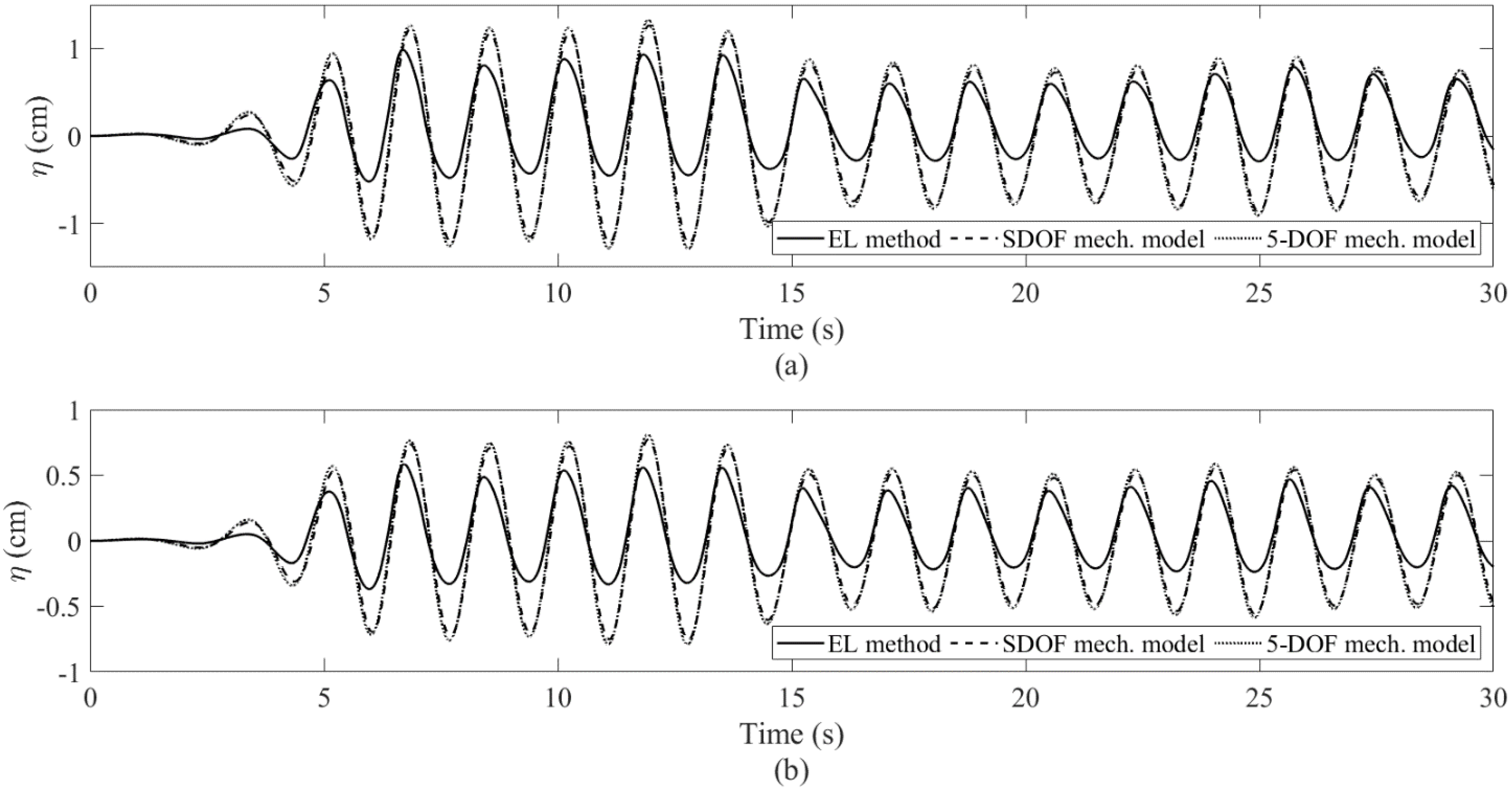
The free-surface elevations on the left-side (stern side) wall of the tank for the large- and small-wave cases are shown in Figure 22. Note that in the mechanical model, the free-surface elevation of the sloshing fluid can be obtained by:

$$\eta ={\displaystyle \sum }_{n=0}^{\infty }\frac{4tanh{a}_{n}h}{a_{n}L}sin{a}_{n}x·x_n$$

(51)

In the large-wave case, the EL method could simulate nonlinear waves. The mechanical model showed linear waves and overestimated the amplitude due to the lack of nonlinear damping. Similar results have been observed in past experiments [25]. In the small-wave case, the wave elevations by both methods were still different. However, it only slightly changed the sloshing forces. Besides, the five-DOF system included more high-mode sloshing responses than the SDOF system. It gave a higher hydrostatic pressure but those components were too small to affect the FSI simulation.

Figure 22. The free-surface elevations on the left-side wall of the tank for different wave loadings: (a) large wave; (b) small wave.

Figure 22. The free-surface elevations on the left-side wall of the tank for different wave loadings: (a) large wave; (b) small wave.

4.2. Floating Body in Resonant Waves: Controlled vs. Uncontrolled

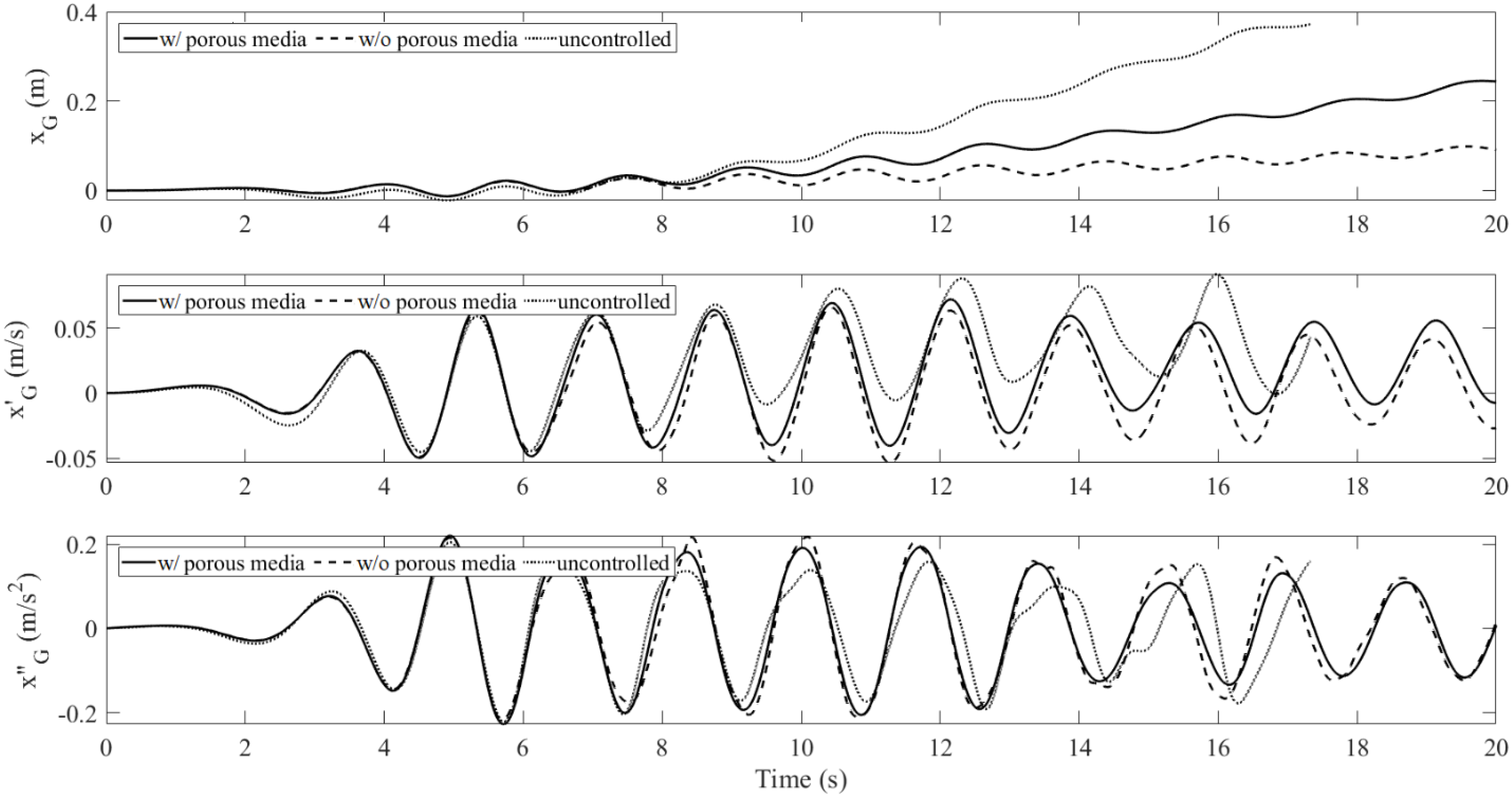
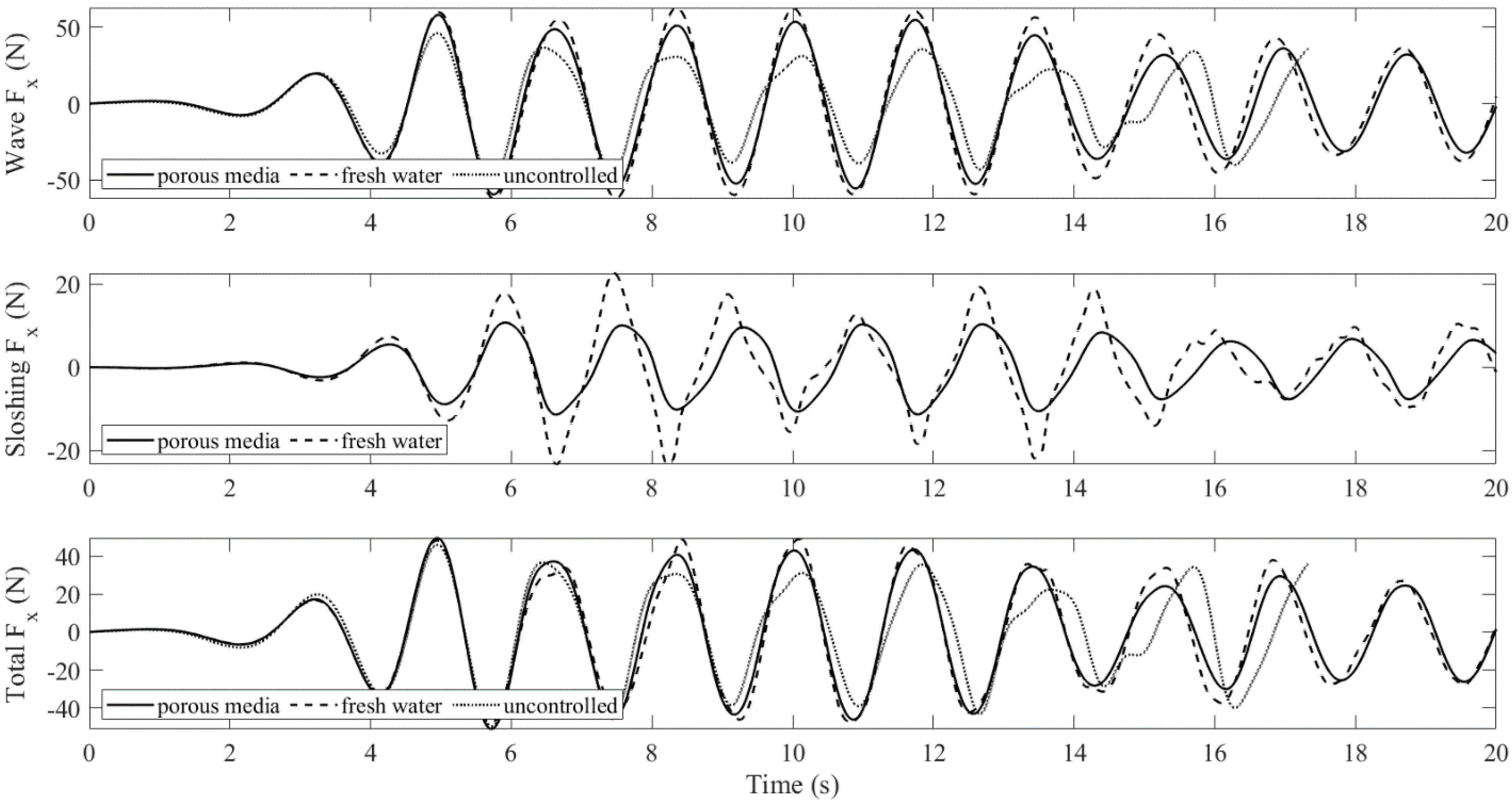
The uncontrolled body means that no water tank was installed on the platform, otherwise, it is called a controlled body. For the controlled body, an additional case is considered where the tank was only filled with water and no porous media, which suggests the porosity $\gamma$ = 1 and the coefficients ${\alpha }_1$ = 0.1 s⁻¹ and ${\alpha }_2$ = 0 m⁻¹ were used in the EL method [46]. When the large wave was applied, the body motions and the resultant forces along the horizontal direction are shown in Figure 23 and Figure 24, respectively. The uncontrolled case stopped at 17.3 s due to the numerical instability induced by the high velocity of a wave jet on the body. The water tank was prone to keep the floating body oscillating around the original position, hence it could slow down the lateral drift. Although the force cancellation was weak, it still reduced the surge motion. However, the floating body was free to surge in our case, and the effectiveness of the surge mitigation by the porous media in the sloshing fluid was not obvious.

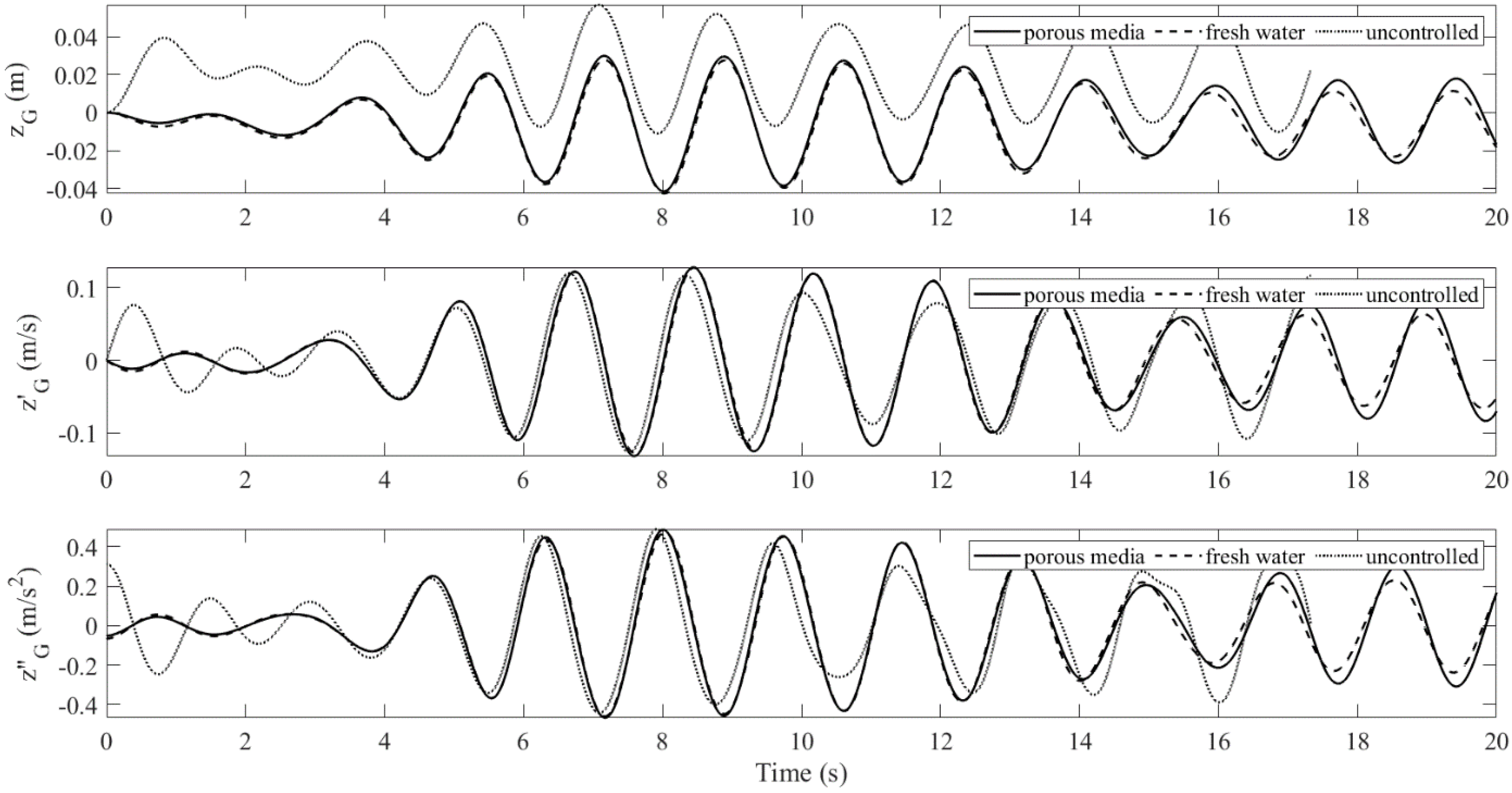
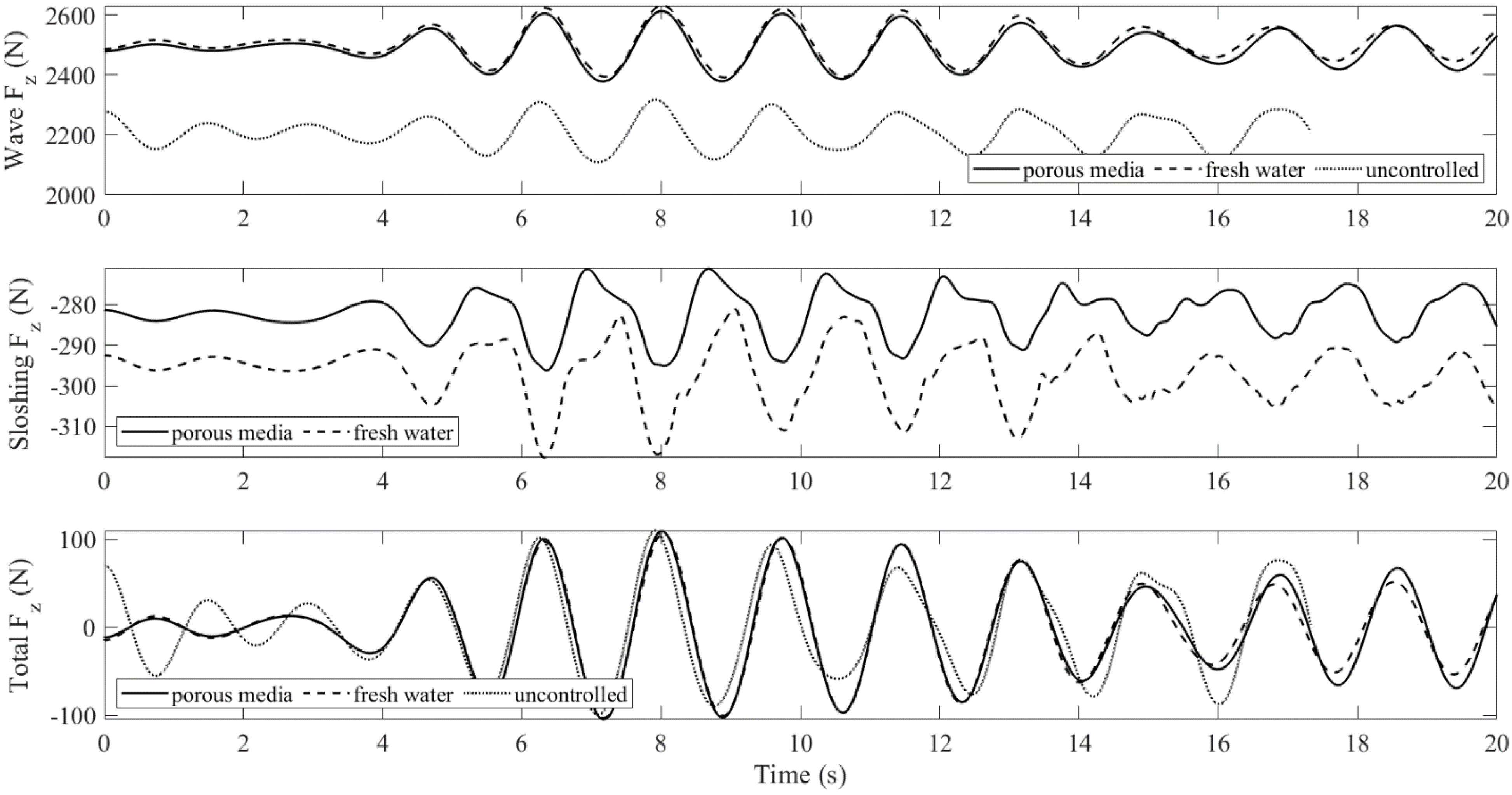
The body motions and the resultant forces along the vertical direction are shown in Figure 25 and Figure 26, respectively. The mean values of the steady-state displacement were different for the controlled and uncontrolled cases because their total weights were different. The uncontrolled body was lighter, so it had a larger initial acceleration. As their transient response vanished, they oscillated in the same way but had different equilibrium points. This implies that the sloshing fluid did not change the heave motion of the body. Besides, the difference between the vertical sloshing forces from the tanks with and without porous media equaled their difference in water weight. The porous media did not affect the vertical sloshing force.

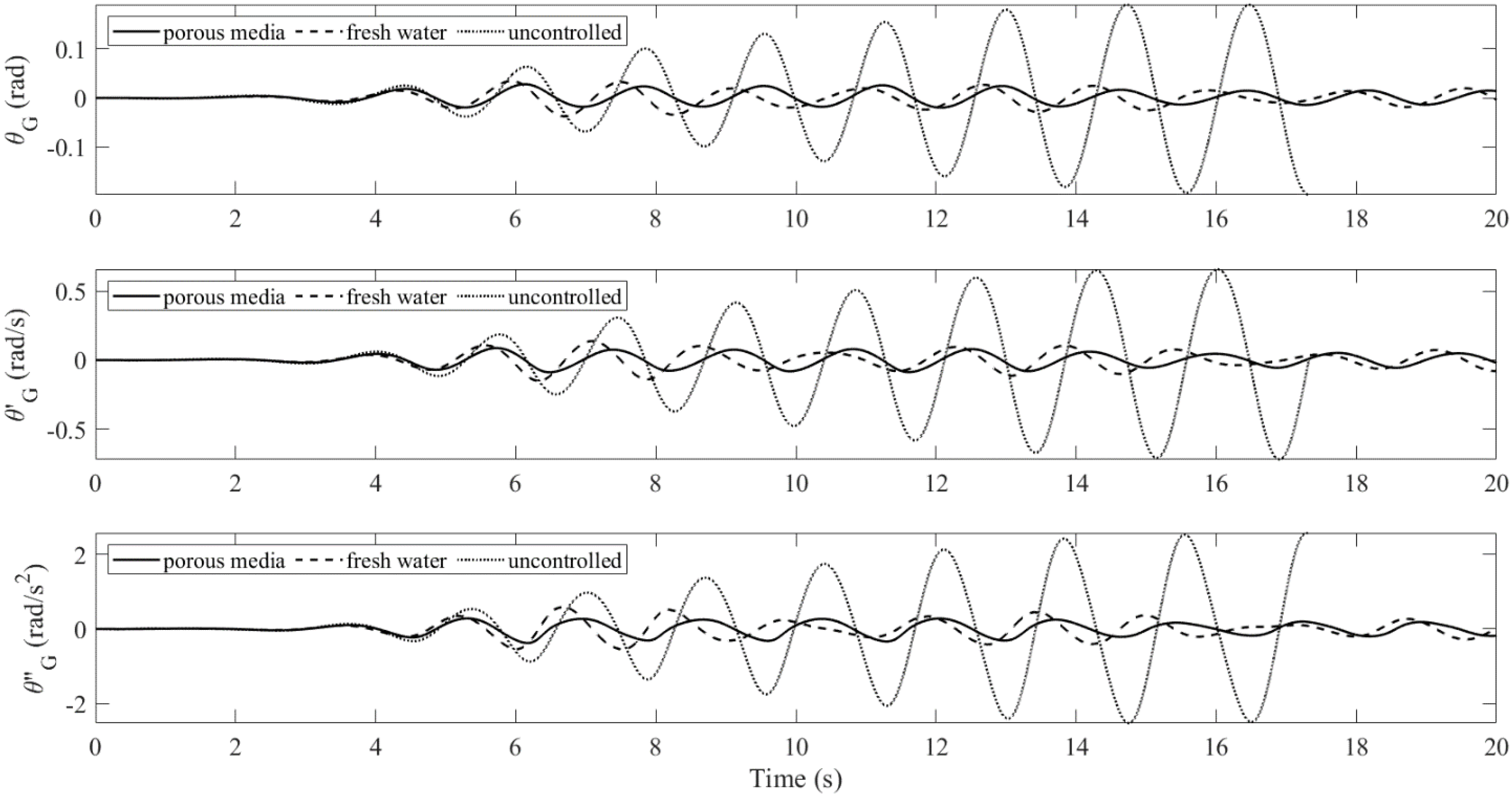
The body motions and the resultant forces about the angular axis are shown in Figure 27 and Figure 28, respectively. For the uncontrolled case, the responses were greatly amplified due to resonance. The maximum angular displacement was 11.3°. In the controlled cases, the maximum angular displacements were significantly reduced to 2.2° (without porous media) and 1.6° (with porous media). Moreover, their transient responses decayed very fast and the steady-state responses were suppressed. This can be explained later by the energy exchange in the body-tank system. The force cancellation between the sloshing reaction and wave loading was strong, showing that the tuning condition may have been satisfied. The tank with porous media had better performance in reducing pitch vibration than the other tank, but the overall performance should be validated through other near-resonance tests in the next example.

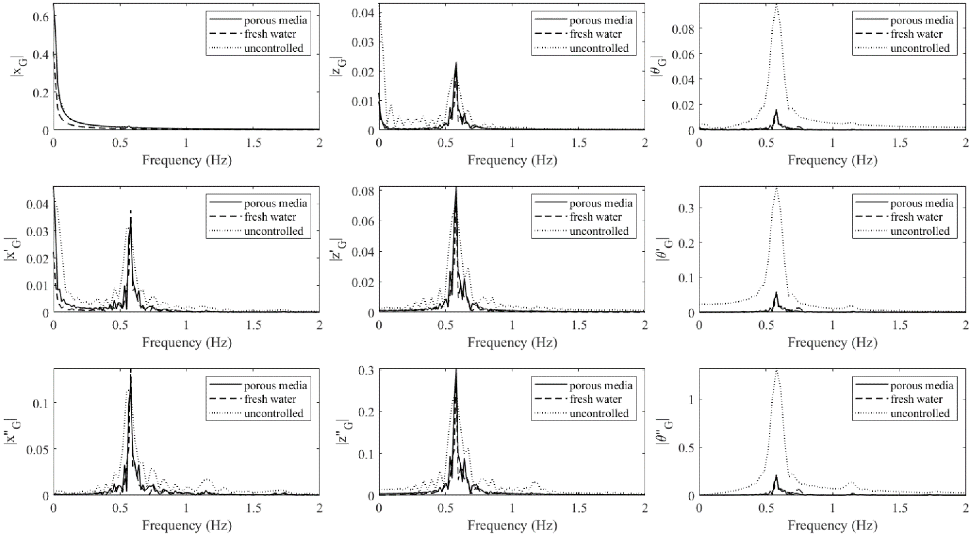
The response spectra of the controlled and uncontrolled floating bodies subject to large wave excitation are shown in Figure 29. The major oscillatory frequency does not shift (still 0.58 Hz), while a small local peak shows up at the frequency of 0.53 Hz, which is equal to the natural frequency of the sloshing fluid in the tank. The dynamic characteristic of the entire system was not affected because the water tank was not heavy enough (the mass ratio was 13%). The maximum amplitudes of the angular responses of the floating body were greatly decreased. Compared to the tank without porous media, the porous media could further reduce the peak response of the surge and pitch motions.

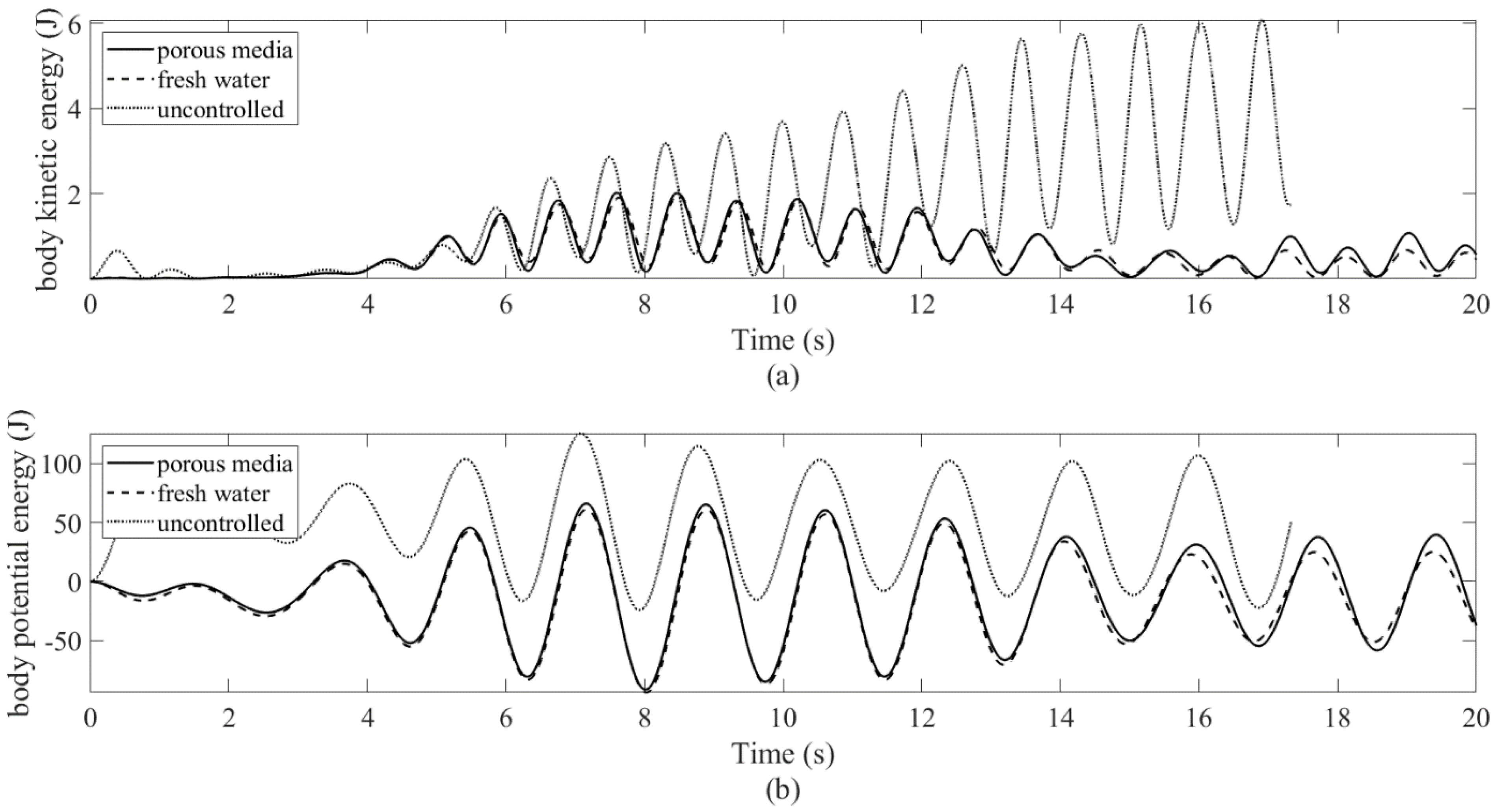
The kinetic energy and potential energy of the floating body and sloshing fluid can be obtained by:

$$T_b=\frac{1}{2}{M}_b{\left|{\dot{x}}_G\right|}^2+\frac{1}{2}{I}_b{\left|{\dot{\theta }}_G\right|}^2 and T_s=\frac{1}{2}{{\displaystyle \int }}_{S_1}^{}\gamma \rho \varphi \frac{\partial \varphi }{\partial n}dS$$

(52)

$$V_b=M_{b}g{z}_G and V_s=\frac{1}{2}\gamma \rho g{{\displaystyle \int }}_{S_{f1}}^{}{\eta }^{2}dS$$

(53)

where the subscripts b and s denote the floating body and sloshing fluid, respectively. Note that $T_s$ is obtained by applying Green’s identity to the volume integral of the kinetic energy of a fluid particle [47]. The zero-potential plane is defined at z = 0. The changes in the kinetic and potential energy, i.e., the difference between the energy at current and initial states of the floating body are shown in Figure 30. In Figure 30a, the kinetic energy increased rapidly because the body velocity increased when the incident wave came. For the controlled case, the water tank dampened the transient vibrations, so the body’s kinetic energy reached the steady state quickly. It is noticeable that the kinetic energy of the body without porous media was lower than that with porous media because of the lower heaving velocity, as shown in Figure 25. However, the porous media dampened more body kinetic energy from the surge and pitch components. Figure 25 and Figure 30b show that the potential energy change was in sync with the vertical displacement. Since the water tank did not mitigate the heaving motion, the potential energy change of the body was irrelevant to the sloshing behavior and only depended on the vertical force equilibrium.

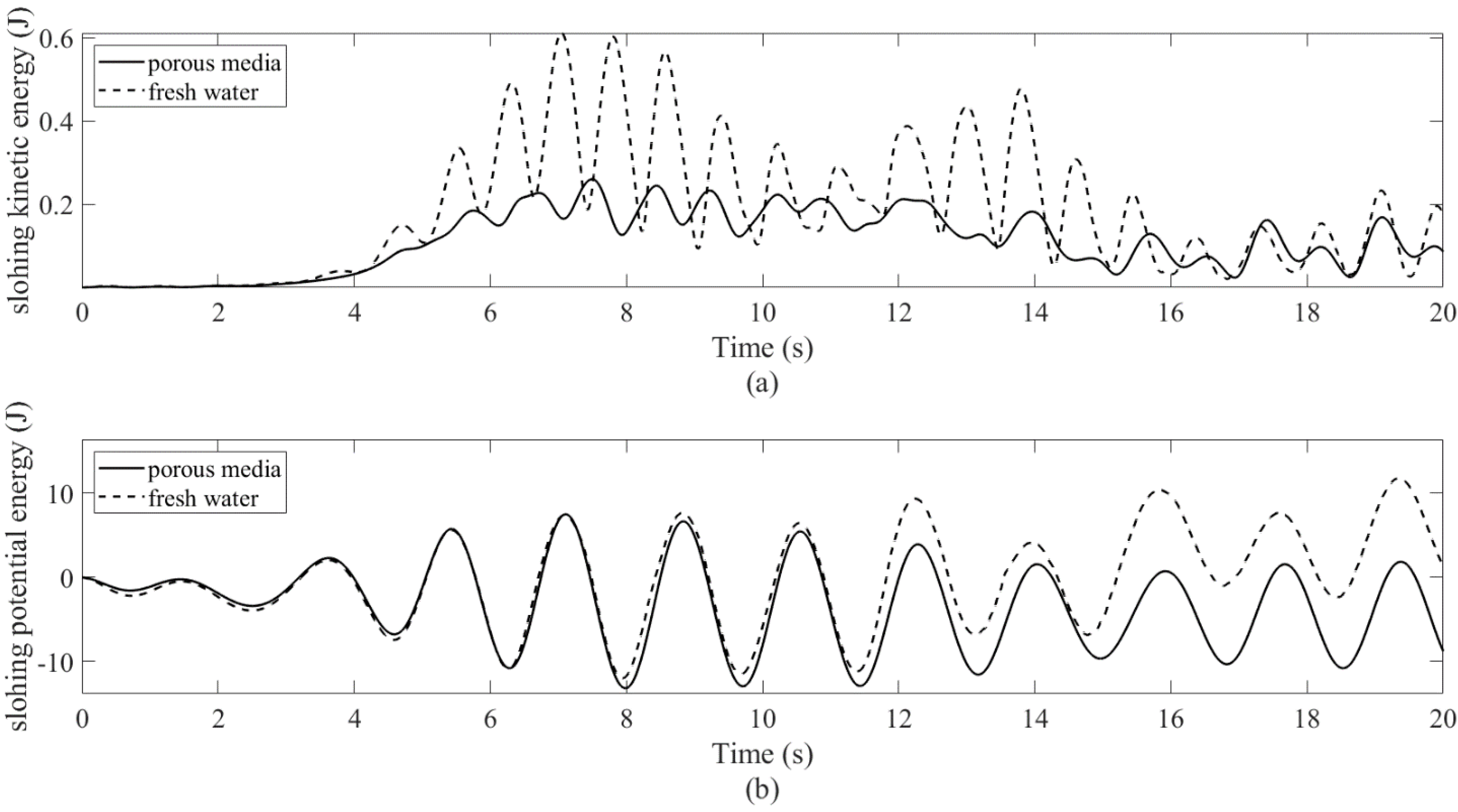
The kinetic and potential energy changes of the sloshing fluid are shown in Figure 31. For the first 15 s in Figure 31a, the kinetic energy of the sloshing fluid without porous media increased faster than that with porous media. This shows the porous media can quickly dampen the kinetic energy in the transient state, therefore suppressing the fluid velocity and the free-surface deformation. By correlating the force/moment and energy change as shown in Figure 24, Figure 28, Figure 30 and Figure 31, the effect of porous media on the FSI can be characterized. When the incident waves hit the floating body, the work is transferred to the body’s kinetic energy. Through the force cancellation, part of the wave-induced work will be taken by the sloshing fluid, and then dissipated by the damping mechanism of the porous media. Therefore, good force cancellation and enough sloshing damping are two key factors for structural vibration control. In Figure 31b, the potential energy of the fluid in the tank without porous media grew higher than that of the fluid in the porous media. Since they had similar elevations, the difference in the potential energy came from different free-surface deformations.

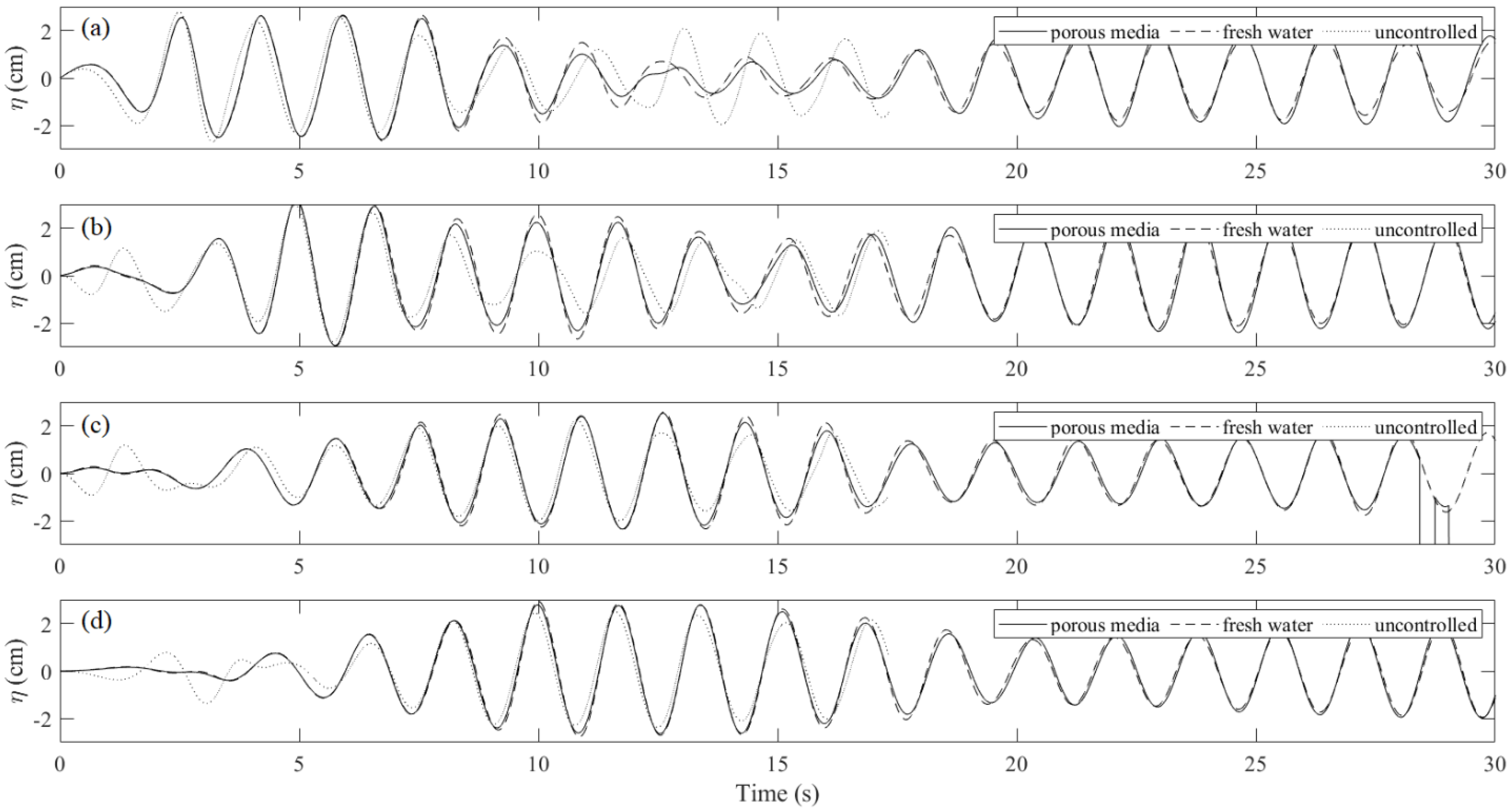
The free-surface elevations on the left-side wall of the tank with and without porous media are shown in Figure 32. The wave elevation in the tank without porous media was very nonlinear, while the porous media reduced the degree of nonlinearity due to their extra damping effect. This shows the benefit for the liquid storage tank that not only the dynamic pressure can be reduced, but the roof damage can be alleviated.

The wave elevations of four gauges distributed at x = 2, 4, 6, and 8 m (two on the left side and two on the right side of the body) along the channel are shown in Figure 33. At the beginning (t < 2 s), the incident wave had not reached the body, so the body only oscillated vertically. The uncontrolled body had a larger initial acceleration, so it induced a larger disturbance to the waves, as shown in Figure 33b,c. The heave-induced wave that propagated downstream was recorded as is shown in Figure 33d. However, there was no significant change in the first gauge because of the overwhelming incident waves. As the incident wave reached the floating body (t > 2 s), the body started to surge and pitch. In our case, the wavelength was about 4.6 m, which was close to the distance between the wavemaker and the body. Therefore, a standing wave occurred so larger wave elevations at gauge two during t = 2~10 s were observed, as shown in Figure 33b. The influence on the far-distance wave field due to the body motion was negligible, as shown in Figure 33d.

4.3. Frequency Response Analysis

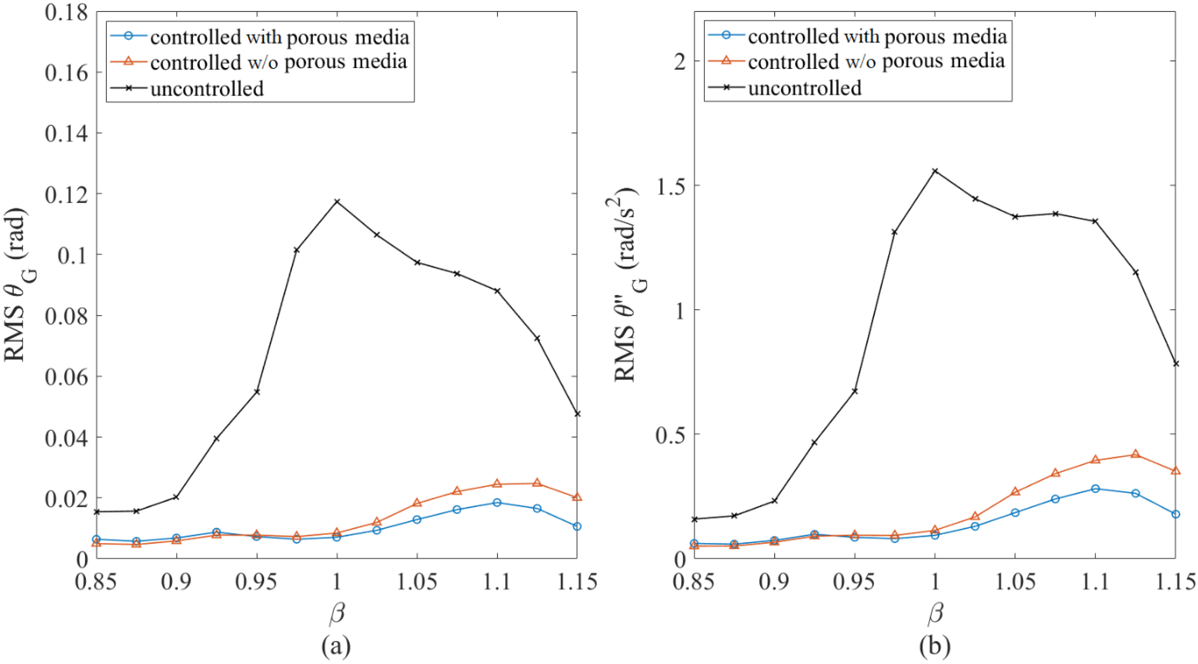
To complete the frequency response curves, the near-resonance condition was emphasized in the range of $\beta$ = 0.85~1.15, where $\beta$ is the ratio between the frequencies of the wavemaker’s movement and the body’s pitch motion. The small wave excitation was applied to avoid unstable numerical results in uncontrolled cases. For the first application of structural control, the water tank was installed as a TLD. The frequency responses of the root-mean-square (RMS) of the steady-state angular displacement and acceleration of the body are shown in Figure 34. TLDs can enhance the workability and comfort of the workstation. The average reduction in the RMS displacement and acceleration by the porous-media TLD was 85%, while that by the fresh-water TLD (TLD without porous media) was 80%. However, the porous-media TLD showed at least 10% better performance than the fresh-water one in the high-frequency range ($\beta$ ≥ 1.075). This is because the high nonlinearity of the fresh-water TLD can cause a strong mistuning effect. Once the natural frequency of the water tank deviates from the tuning frequency too much, the force cancellation will be weakened. In terms of the tuning condition, the porous-media TLD can be optimized more easily according to a simple design plan [22]. A single peak occurred at $\beta$ = 1 in uncontrolled cases, while there were two peaks at $\beta$ = 0.925 and 1.1 when the TLD was installed. Theoretically, the sloshing fluid had infinite degrees of freedom. Therefore, the body-tank system was a multi-degree-of-freedom system. Since the fundamental sloshing mode dominated (as was concluded in the previous example), the frequency response curves only had two peaks that represented two major vibration modes of the TLD-body system.

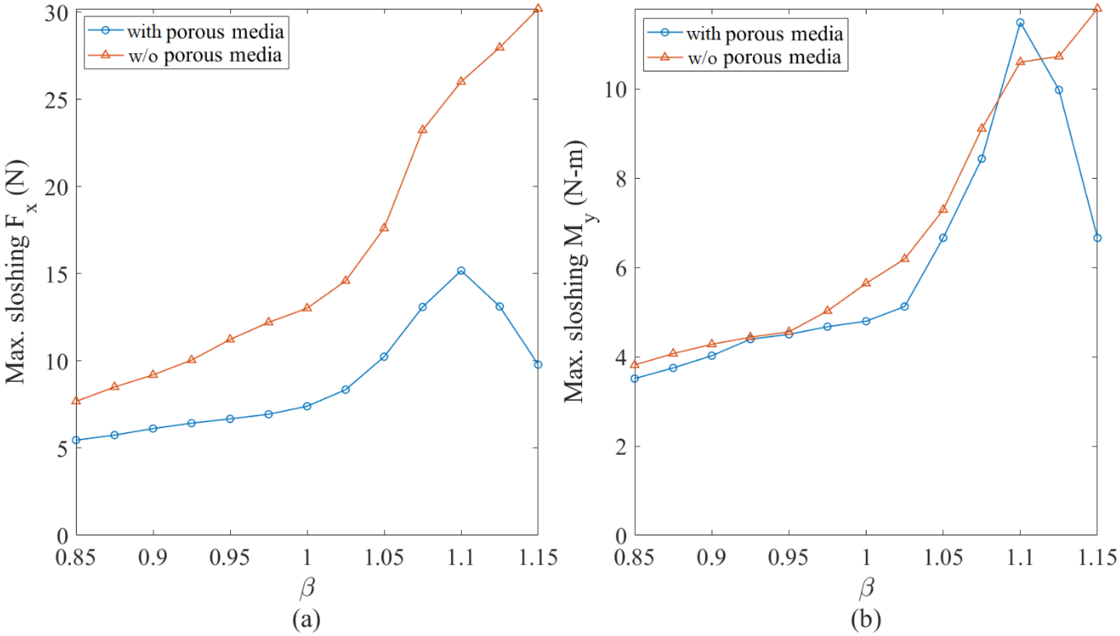
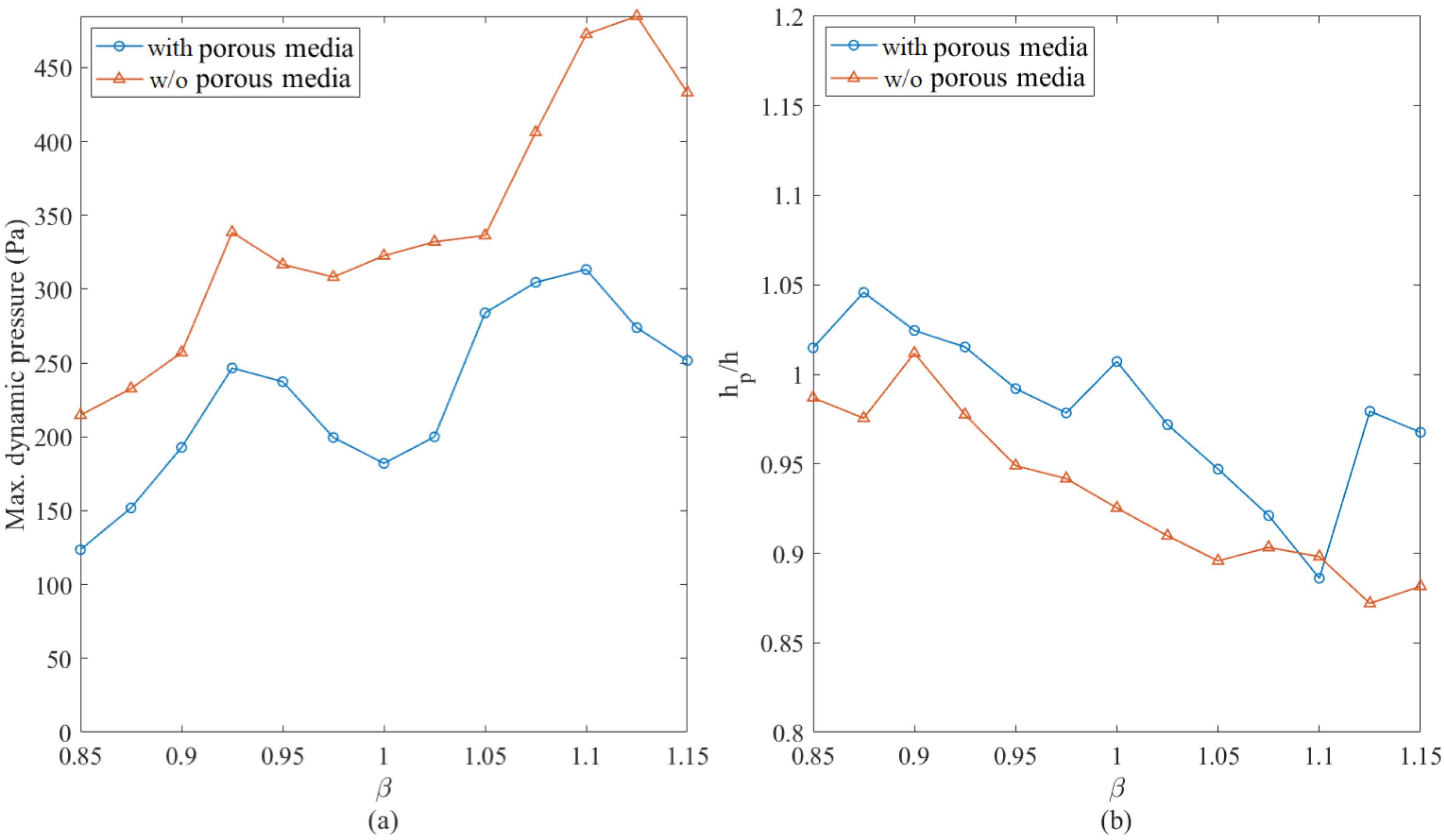
For a liquid carrier on the ocean, its stability is related to the amplitude of the wave-induced sloshing resultants. The frequency responses of the maximum horizontal force and overturning moment due to sloshing fluid are shown in Figure 35. In Figure 35a, the porous media can reduce the horizontal force by 30~70% because the extra damping effect limits the sloshing responses, hence reducing the hydrodynamic force. In Figure 35b, the reduction in the overturning moment was low. This is because, for a shallow-water tank used in this example, the overturning moment did not mainly come from the horizontal component. Therefore, the reduction by the porous media was not obvious. The integrity of a liquid container is another important issue that is related to pressure concentration. The frequency responses of the maximum dynamic pressure on the wetted wall and the normalized height of the local maximum pressure are shown in Figure 36. Note that $h_p$ denotes the elevation of the fluid particle that has the maximum dynamic pressure. In Figure 36a, the maximum dynamic pressure in the tank without porous media was 485 Pa, which was higher than the maximum hydrostatic pressure (460 Pa). The porous media reduced 25~45% of the dynamic pressure. The averages were 343 versus 228 Pa. In Figure 36b, the elevations of the local maximum pressure were similar, which were below the still-water line (h_p/h < 1) in most cases. As the wave traveled back and forth during the vibration, the greatest impact occurred at the instant when it reached the walls. The contact location was usually near but below the still-water line. This phenomenon was visualized in the past article [48]. Overall, the porous media will not change the location of the pressure concentration but can effectively reduce the hydrodynamic pressure.

5. Conclusions

From this study, some conclusions can be drawn:

• Porous media can accelerate the energy transmission in the FSI process, enhance the damping capability of the sloshing fluid, and reduce the sloshing velocity and deformation.
• The sloshing fluid will create a control force on the body. Under certain circumstances, it will cancel the wave loading. When it happens, the work done by incident waves is transferred to the fluid in the water tank (meanwhile, the wave-induced sloshing behavior appears), and then dissipated by the damping mechanism of porous media.
• The mechanical model produces linear sloshing reactions, which affects the accuracy of the amplitude of the body’s pitch motion for the large-wave case. However, it still captures the oscillatory frequencies very well. For the small-wave case, the difference is insignificant. When the tank is subject to pitch motion, the first modal sloshing response dominates.
• In the near-resonance tests, the average reduction in the RMS pitch motion by the porous-media TLD was 85%. It did not produce an effective control force for the heave motion. Moreover, the force cancellation in the horizontal motion was weak. Therefore, the application in surge mitigation is uncertain. Compared to the fresh-water TLD, the mistuning effect was alleviated.
• Porous media can effectively decrease the hydrodynamic pressure by up to 45%. The integrity of the liquid container and the stability of the liquid carrier can be improved.

References

- Cariou, A.; Casella, G. Liquid sloshing in ship tanks: A comparative study of numerical simulation. Mar. Struct. 1999, 12, 183–198. [Google Scholar] [CrossRef]
- Kim, Y.; Nam, B.W.; Kim, D.W.; Kim, Y.S. Study on coupling effects of ship motion and sloshing. Ocean Eng. 2007, 34, 2176–2187. [Google Scholar] [CrossRef]
- Lee, S.J.; Kim, M.H.; Lee, D.H.; Kim, J.W.; Kim, Y.H. The effects of LNG-tank sloshing on the global motions of LNG carriers. Ocean Eng. 2007, 34, 10–20. [Google Scholar] [CrossRef]
- Lyu, W.J.; Riesner, M.; Peters, A.; Moctar, O. A hybrid method for ship response coupled with sloshing in partially filled tanks. Mar. Struct. 2019, 67, 102643. [Google Scholar] [CrossRef]
- Burger, W.; Corbet, A.G. Chapter III—Anti-Rolling Devices in General. In Ship Stabilizers: A Handbook for Merchant Navy Officers; 1966; pp. 31–37. Available online: https://0-www-sciencedirect-com.brum.beds.ac.uk/science/article/pii/B9780080115047500095 (accessed on 1 May 2022).
- Chen, Y.H.; Ko, C.H. Active tuned liquid column damper with propellers. Earthq. Eng. Struct. Dyn. 2003, 32, 1627–1638. [Google Scholar] [CrossRef]
- Yalla, S.K.; Kareem, A.; Kantor, J.C. Semi-active tuned liquid column dampers for vibration control of structures. Eng. Struct. 2001, 23, 1469–1479. [Google Scholar] [CrossRef]
- Marzouk, O.A.; Nayfeh, A.H. Control of ship roll using passive and active anti-roll tanks. Ocean Eng. 2009, 36, 661–671. [Google Scholar] [CrossRef]
- Gattulli, V.; Ghanem, R. Adaptive control of flow-induced oscillations including vortex effects. Int. J. Non-Linear Mech. 1999, 34, 853–868. [Google Scholar] [CrossRef]
- Kawano, K. Active control effects on dynamic response of offshore structures. In Proceedings of the Third International Offshore and Polar Engineering Conference, Singapore, 6–11 June 1993; pp. 594–598. [Google Scholar]
- Stewart, G.; Lackner, M. Offshore wind turbine load reduction employing optimal passive tuned mass damping systems. IEEE Trans. Control Syst. Technol. 2013, 21, 1090–1104. [Google Scholar] [CrossRef]
- Si, Y.; Karimi, H.R.; Gao, H. Modelling and optimization of a passive structural control design for a spar-type floating wind turbine. Eng. Struct. 2014, 69, 168–182. [Google Scholar] [CrossRef]
- Dinh, V.N.; Basu, B. Passive control of floating offshore wind turbine nacelle and spar vibrations by multiple tuned mass dampers. Struct. Control Health Monit. 2014, 22, 152–176. [Google Scholar] [CrossRef]
- Tong, X.; Zhao, X.; Karcanias, A. Passive vibration control of an offshore floating hydrostatic wind turbine model. Wind Energy 2018, 21, 697–714. [Google Scholar] [CrossRef] [Green Version]
- Chen, J.; Zhan, G.; Zhao, Y. Application of spherical tuned liquid damper in vibration control of wind turbine due to earthquake excitations. Struct. Des. Tall Spec. Build. 2016, 25, 431–443. [Google Scholar] [CrossRef]
- Chen, Y.H.; Hwang, W.S.; Tsao, W.H. Nonlinear dynamic characteristics of rectangular and cylindrical TLD’s. J. Eng. Mech. 2018, 144, 06018004. [Google Scholar] [CrossRef]
- Zahrai, S.M.; Abbasi, S.; Samali, B.; Vrcelj, Z. Experimental investigation of utilizing TLD with baffles in a scaled down 5-story benchmark building. J. Fluids Struct. 2012, 28, 194–210. [Google Scholar] [CrossRef]
- Warnitchai, P.; Pinkaew, T. Modelling of liquid sloshing in rectangular tanks with flow-dampening devices. Eng. Struct. 1998, 20, 293–600. [Google Scholar] [CrossRef]
- Faltinsen, O.M.; Firoozkoohi, R.; Timokha, A.N. Analytical modeling of liquid sloshing in a two-dimensional rectangular tank with a slat screen. J. Eng. Math. 2011, 70, 93–109. [Google Scholar] [CrossRef] [Green Version]
- Hamelin, J.; Love, J.; Tait, M.; Wison, J. Tuned liquid dampers with a Keulegan-Carpenter number-dependent screen drag coefficient. J. Fluids Struct. 2013, 43, 271–286. [Google Scholar] [CrossRef]
- Tait, M.J. Modelling and preliminary design of a structure-TLD system. Eng. Struct. 2008, 30, 2644–2655. [Google Scholar] [CrossRef]
- Tsao, W.H.; Hwang, W.S. Tuned liquid dampers with porous media. Ocean Eng. 2018, 167, 55–64. [Google Scholar] [CrossRef]
- Tsao, W.H.; Hwang, W.S. Dynamic characteristics of liquid sloshing in cylindrical tanks filled with porous media. In IOP Conference Series: Earth and Environmental Science; IOP Publishing: Bristol, UK, 2019; Volume 351. [Google Scholar]
- Tsao, W.H.; Chang, T.J. Sloshing phenomenon in rectangular and cylindrical tanks filled with porous media: Supplementary solution and impulsive-excitation experiment. J. Eng. Mech. 2020, 146, 04020139. [Google Scholar] [CrossRef]
- Tsao, W.H.; Huang, L.H.; Hwang, W.S. An equivalent mechanical model with nonlinear damping for sloshing rectangular tank with porous media. Ocean Eng. 2021, 242, 110145. [Google Scholar] [CrossRef]
- Tsao, W.H.; Huang, Y.L. Sloshing force in a rectangular tank with porous media. Results Eng. 2021, 11, 100250. [Google Scholar] [CrossRef]
- Sen, D. Numerical simulation of motions of two-dimensional floating bodies. J. Ship Res. 1993, 37, 307–330. [Google Scholar] [CrossRef]
- Van Daalen, E.F.G. Numerical and Theoretical Studies of Water Waves and Floating Bodies. Ph.D. Thesis, Universiteit Twente, Enschede, The Netherlands, 1993. [Google Scholar]
- Tanizawa, K. A nonlinear simulation method of 3D body motions in waves. J. Soc. Nav. Archit. Jpn. 1995, 178, 179–191. [Google Scholar] [CrossRef]
- Jung, K.H.; Chang, K.A.; Jo, H.J. Viscous effect on the roll motion of a rectangular structure. J. Eng. Mech. 2006, 132, 190–200. [Google Scholar] [CrossRef]
- Guerber, E.; Benoit, M.; Grilli, S.T.; Buvat, C. A fully nonlinear implicit model for wave interactions with submerged structures in forced or free motion. Eng. Anal. Bound. Elem. 2012, 36, 1151–1163. [Google Scholar] [CrossRef] [Green Version]
- Dombre, E.; Benoit, M.; Violeau, D.; Peyrard, C.; Grilli, S.T. Simulation of floating structure dynamics in waves by implicit coupling of a fully non-linear potential flow model and a rigid body motion approach. J. Ocean Eng. Mar. Energy 2015, 1, 55–76. [Google Scholar] [CrossRef] [Green Version]
- Vinje, T.; Brevig, P. Nonlinear, Two-Dimensional Ship Motions; Technical Report; Norwegian Institute of Technology: Trondheim, Norway, 1981; p. R-112.81. [Google Scholar]
- Belibassakis, K.A. A boundary element method for the hydrodynamic analysis of floating bodies in variable bathymetry regions. Eng. Anal. Bound. Elem. 2008, 32, 796–810. [Google Scholar] [CrossRef]
- Wu, G.X.; Eatock-Taylor, R. Transient motion of a floating body in steep water waves. In Proceedings of the 11th Workshop on Water Waves and Floating Bodies, Hamburg, Germany, 17–20 March 1996. [Google Scholar]
- Matthies, H.G.; Niekamp, R.; Steindorf, J. Algorithms for strong coupling procedures. Comput. Methods Appl. Mech. Eng. 2006, 195, 2028–2049. [Google Scholar] [CrossRef]
- Palm, J.; Eskilsson, C.; Paredes, G.M.; Bergdahl, L. Coupled mooring analysis of floating wave energy converters using CFD: Formulation and Validation. Int. J. Mar. Energy 2016, 16, 83–99. [Google Scholar] [CrossRef] [Green Version]
- Tezduyar, T.E. Finite element methods for flow problems with moving boundaries and interfaces. Comput. Methods Eng. 2001, 8, 83–130. [Google Scholar] [CrossRef]
- Rakhsha, M.; Kees, C.E.; Negrut, D. Lagrangian vs. Eulerian: An analysis of two solution methods for free-surface flows and fluid solid interaction problems. Fluids 2021, 6, 460. [Google Scholar] [CrossRef]
- Karimirad, M.; Michailides, C.; Nematbakhsh, A. Offshore Mechanics: Structural and Fluid Dynamics for Recent Applications. 2018. Available online: https://0-www-wiley-com.brum.beds.ac.uk/en-us/Offshore+Mechanics%3A+Structural+and+Fluid+Dynamics+for+Recent+Applications-p-9781119216629 (accessed on 1 May 2022).
- Grilli, S.T.; Skourup, J.; Svendsen, I.A. An efficient boundary element method for nonlinear water waves. Eng. Anal. Bound. Elem. 1989, 6, 97–107. [Google Scholar] [CrossRef]
- Grilli, S.T.; Horrillo, J. Numerical generation and absorption of fully nonlinear periodic waves. J. Eng. Mech. 1997, 123, 1060–1069. [Google Scholar] [CrossRef] [Green Version]
- Tsao, W.H.; Kinnas, S.A. Local simulation of sloshing jet in a rolling tank by viscous-inviscid interaction method. Results Eng. 2021, 11, 100270. [Google Scholar] [CrossRef]
- Nield, A.D.; Bejan, A. Convection in Porous Media, 4th ed.; Springer: New York, NY, USA, 2013. [Google Scholar]
- Ursell, F.; Dean, R.G.; Yu, Y.S. Forced small-amplitude water waves: A comparison of theory and experiment. J. Fluid Mech. 1960, 7, 33–52. [Google Scholar] [CrossRef]
- Chen, Y.H.; Hwang, W.S.; Tsao, W.H. Nonlinear sloshing analysis by regularized boundary integral method. J. Eng. Mech. 2017, 143, 040170046. [Google Scholar] [CrossRef]
- Currie, I.G. Fundamental Mechanics of Fluids, 3rd ed.; CRC Press: Boca Raton, FL, USA, 2003. [Google Scholar]
- Delorme, L.; Colagrossi, A.; Souto-Iglesias, A.; Zamora-Rodríguez, R.; Botia-Vera, E. A set of canonical problems in sloshing, Part I: Pressure field in forced roll comparison between experimental results and SPH. Ocean Eng. 2009, 36, 168–178. [Google Scholar] [CrossRef]
Figure 3.
The horizontal displacement, velocity, and acceleration time histories of the floating body under free vibration at an initial 5° pitch.
Figure 4.
The vertical displacement, velocity, and acceleration time histories of the floating body under free vibration at an initial 5° pitch.
Figure 5.
The angular displacement, velocity, and acceleration time histories of the floating body under free vibration at an initial 5° pitch.
Figure 6.
The response spectra of the floating body under free vibration at an initial 5° pitch.
Figure 7.
The numerical configurations for (a) EL method; (b) mechanical model, in the FSI problem (not to scale).