Analytic Derivation of Ascent Trajectories and Performance of Launch Vehicles

Abstract

This papers introduces an analytic method to define multistage launcher trajectories to determine the payload mass that can be inserted in orbits of different semimajor axes and inclinations. This method can evaluate the gravity loss, which is the main term to be subtracted to the Tziolkowski evaluation of the velocity provided by the thrust of a launcher. In the method, the trajectories are dependent on two parameters only: the final flight-path angle ${\gamma }_f$ at the end of the gravity-turn arc of the launcher trajectory and the duration $t_c$ of the coasting arc following the gravity-turn phase. The analytic formulas for the gravity-turn phase, being solutions of differential equations with a singularity, allow us to identify the trajectory with a required final flight-path angle ${\gamma }_f$ in infinite solutions with the same initial vertical launch condition. This can also drive the selection of the parameters of the pitch manoeuvre needed to turn the launcher from the initial vertical arc. For any pair ${\gamma }_f$ and $t_c$, a launcher trajectory is determined. A numerical solver is used to identify the values ${\gamma }_f$ and $t_c$, allowing for the insertion of the payload mass into the required orbit. The analytic method is compared with a numerical code including the drag effect, which is the only effect overlooked in the analytic formulas. The analytical method is proven to predict the payload mass with an error never exceeding the 10% of the actual payload mass, found through numerical propagation.

1. Introduction

The number of microsatellites to be orbited is increasing rapidly, in particular for the delivery and replacement of microsatellites as part of mega constellation programs. This is stimulating a new wave of dedicated launch vehicles capable of offering responsive, flexible and cost-effective services to this huge and new market. Some of these “micro-launchers” are listed in

Table 1. Listof Micro-Launchers.

Launcher	Total Mass	Number of Stages	Max Payload to LEO	Maiden Flight
Simorgh, Iran	78,926 kg	3	350 kg	2021
Unha, North Korea	68,039 kg	3	200 kg	2012
LongMarc11, China	58,000 kg	4	700 kg	2015
Spectrum, Germany	50,000 kg	2	950 kg	2022 (planned)
Minotaur1, USA	36,200 kg	4	580 kg	2000
Zhu-Que1, China	24,600 kg	3	300 kg	2018
LauncherOne, USA	23,410 kg	2	500 kg	2000
Quased, Iran	22,700 kg	3	50 kg	2020
Kuoizhou1A, China	15,100 kg	3	300 kg	2017
Electron, USA	11,400 kg	2	225 kg	2017
Astra R3, USA	9980 kg	2	150 kg	2020

. The mass of payload $m_{pay}$ to be inserted into LEO is below 1000 kg. In fact, $m_{pay}$ is the driving element of a space rocket and it is important to define it at the first step of a launcher design. A very popular method of computation of $m_{pay}$ is offered by the Tziolkowski formula. However, the results obtained using this method are not accurate since the space environment (gravity and aerdoynamic forces) and the guidance (direction of thrust) are not taken into account. On the other hand, the accurate computation of a launcher trajectory and the evaluation of launcher performances is a typical and complex problem in the optimization of aerospace trajectories. Launcher performances are evaluated maximizing the final mass that can be set into orbits with different parameters (semimajor axis, eccentricity, inclination). The problem has initial- and final-state variable constraints, path constraints and discontinuities in the mass variation, due to stage separation. This optimization problem can be approached in different ways: all the approaches require educated guesses to initialize some iterative algorithm able to refine the initial guesses and to achieve the optimal solution.

In the scientific literature, some papers [1,2,3,4,5,6,7] address the problem of optimizing the ascent trajectory of launch vehicles through indirect approaches. Examples are the multiple-subarc gradient restoration algorithm, proposed by Miele, and multiple shooting techniques [5,6,7]. The previously cited works [2,3,4,5,6,7] require a considerable deal of effort for deriving the analytical conditions for optimality and for the subsequent programming and debugging. Furthermore, these methods can suffer from a slow rate of convergence and an excessive dependence on the starting guess. Alternative approaches [8,9] are direct in nature, often are more robust, but require discretization of the problem (e.g., through collocation [8,9]) and the use of dedicated algorithms for nonlinear programming, without avoiding the need of a starting guess. Most recently, the indirect heuristic method [10] was proposed as an effective approach for trajectory optimization of ascent vehicles, with the remarkable feature of not requiring any starting guess. For the purpose of preliminary analysis of the performance of new ascent vehicles, fast, approximate approaches that are exempt from convergence issues and minimize the computational effort are desirable. With this intent, Pontani and Teofilatto [11] and Pallone et al. [12,13] propose two numerical approaches for performance evaluation of multistage launch vehicles that aim at obtaining accurate predictions of the performance attainable from a launch vehicle.

The aim of this paper is to derive formulas, possibly as simple as the Tziolkowski one, able to obtain in a few seconds the performance of a multistage space rockets and also able to offer trajectory parameters useful as input for the convergence of complex numerical programs with accurate representation of the rocket system and its space environment.

The formulas originate from previous work [14], which has been generalized to multistage rockets in [15]; all the rocket state variables are derived in [16]. In the present paper, the method is extended to include the optimal choice of a cost arc and the guidance of the last stage of the launcher till the injection into the selected orbit, so the performance of a space launcher is obtained. The method is based on simple mathematics and physics principles and only a few seconds are needed to determine the payload mass that can be set into orbits of different altitude and inclinations, starting from any location of the launch pad.

The major simplification made in order to obtain these results is that the aerodynamic drag is neglected, and this produces an error in the computation of the launcher trajectories. It is rather difficult to treat the aerodynamic effect analytically due to its highly non-linear dependence on velocity and altitude. Some analytic formulas including aerodynamics are derived in [17]; these however are restricted to the vertical arc of the trajectory. To evaluate the impact of drag, the method presented was compared to numerical results obtained by a high-fidelity level of representation of the launcher dynamics. It is shown that the error in the estimate of the optimal payload mass to be inserted into orbit is relevant only for orbits of altitude below 600 km, and in these cases the error does not exceed 10% Moreover, it is proved that the analytic approach proposed here can provide good guesses for numerical solvers of the optimal control problem.

The paper is organized as follows: in Section 2, a first sizing of a space launcher is given based on the Tziolkowski formula. Assuming a payload mass to be delivered in LEO orbit and assuming a fixed percentage of losses, a method is derived to size the staging of a multistage rocket in an optimal way. In Section 3, analytical formulas for the launcher gravity-turn phase are developed in detail for the case of multiple stage rockets. These formulas provide the launcher trajectory of the first stages and allow for the evaluation of the so-called gravity loss. Section 4 and Section 5 describe the method of computation of the full launcher trajectory till the injection into orbit. Section 6 is dedicated to testing the method with respect to numerical computations.

2. First Sizing of a Launch Vehicle

Achieving a single stage to orbit is still an infeasible task and space launchers have a number N of stages ranging from 2 to 4. Each stage has a total mass $m_i$

$$m_i={m_p}_i+{m_s}_i$$

where ${m_p}_i$ is the propellant contained within the tank of each stage and the structural mass coefficient of each stage is defined as

$${ϵ}_i=\frac{{m_s}_i}{m_i}$$

(1)

The total mass at lift off is

$$M_1={{\Sigma }_{i=1}}^N{m}_i+\left(m_{hs}+m_{pay}\right)$$

with $m_{hs}$ the mass of the heat shields (here released at the end of the gravity-turn phase) and $m_{pay}$ is the satellite mass to be injected into orbit. At the time ${t_b}_1$ of the end of the first stage boost (burn time), the propellant mass ${m_p}_1$ is consumed and the mass of the space rocket is

$${M_1}_f=M_1-{m_p}_1$$

The velocity reached at burn time ${t_b}_1$ can be computed integrating the acceleration

$$\dot{V}=\frac{T}{m}cos\alpha -\frac{\mu }{r^2}sin\gamma -\frac{1}{2}\rho V^2\frac{C_{D}S}{m}$$

(2)

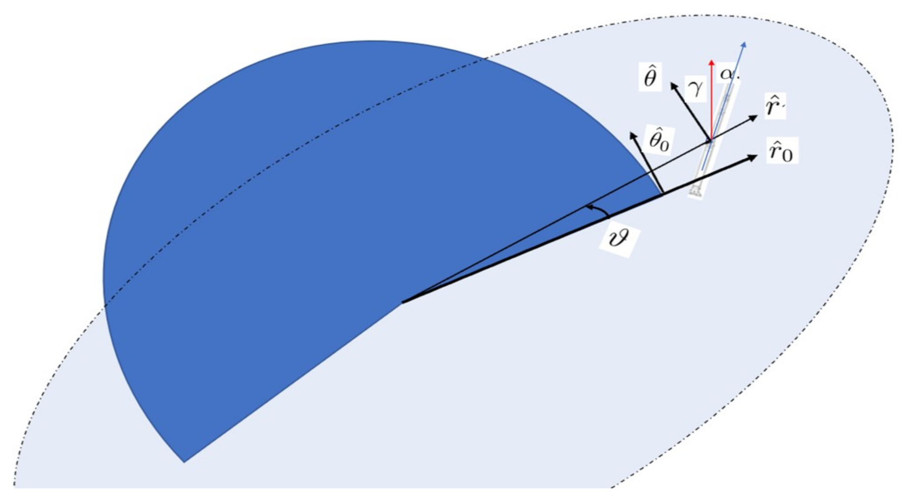
here T is the thrust intensity with a direction determined by the angle $\alpha$ taken from the velocity $\overrightarrow{V}$. The velocity direction is determined by the flight-path angle $\gamma$ taken from the local horizon direction $\widehat{\theta }$, see Figure 1. The variable r is the radius distance from the centre of the Earth to the launcher centre of mass and $\mu$ is the Earth gravitational constant. The atmospheric density is denoted by $\rho$ and $C_D$ is the launcher drag coefficient computed with respect to the reference surface S.

To underline the thrust’s contribution to the variation in velocity and consider all the other terms as “losses”, let us write (2) as

$$\dot{V}=\frac{T}{m}-\frac{\mu }{r^2}sin\gamma -\frac{1}{2}\rho V^2\frac{C_{D}S}{m}-\frac{T}{m}(1-cos\alpha )$$

Integrating the above acceleration between time zero and ${t_b}_1$, one obtains the velocity after the first-stage boost

$$\Delta V_1={{\int }_{t_0}}^{{t_b}_1}\frac{T}{m}dt-{{\int }_{t_0}}^{{t_b}_1}\frac{\mu }{r^2}sin\gamma dt-{{\int }_{t_0}}^{{t_b}_1}\frac{1}{2}\rho V^2\frac{C_{D}S}{m}dt-{{\int }_{t_0}}^{{t_b}_1}\frac{T}{m}(1-cos\alpha )dt$$

(3)

Equation (3) is called the “equation of losses”

$${\Delta V}_1={\Delta V}_{Tz}-{\Delta V}_{grav}-{\Delta V}_{drag}-{\Delta V}_{mis}$$

where the first variation of velocity due to the engine boost is called the Tziolkowski variation of velocity and the other velocities subtracted to ${\Delta V}_{Tz}$ are called gravity, drag and misalignment losses, respectively. Average thrust is defined by $T=gIsp\dot{m}$, where $\dot{m}$ is equal to the mass rate $\dot{m}=-\frac{dm}{dt}$. Inserting $T=-gIsp\frac{dm}{dt}$ in (3), we obtain the Tziolkowski velocity variation provided by the first-stage engine

$$\Delta V_{Tz}=gIsplog\left(\frac{M_1}{{M_1}_f}\right)$$

Introducing the subrocket structural mass ratios

$$U_k=\frac{{M_k}_f}{M_k},M_k={{\Sigma }_{i=k}}^N{m}_i+\left(m_{pay}+m_{hs}\right),{M_k}_f=M_k-{m_p}_k,k=1,N$$

the variation of the velocity provided by the engines of a multistage rocket is

$$\Delta V_{Tz}={\Sigma }_{k=1}^{N}gIs{p}_{k}log\left(\frac{1}{U_k}\right)$$

(4)

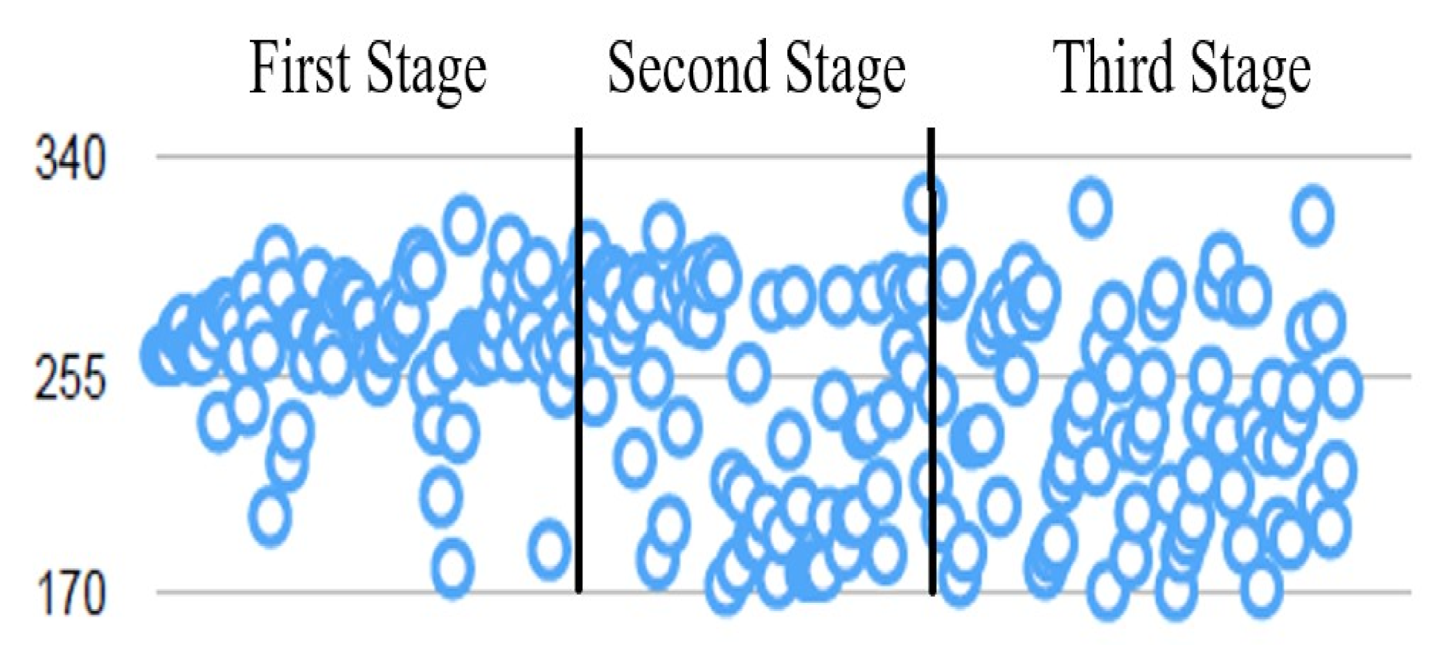
The values of the specific impulses $Is{p}_k$ depend on the kind of propellant, for instance liquid or solid. Figure 2 shows the specific impulses for stages with solid propellant: these values are taken from the database [18] and we have average values

$$Is{p}_1=280s,Is{p}_2=290s,Is{p}_3=270s$$

(5)

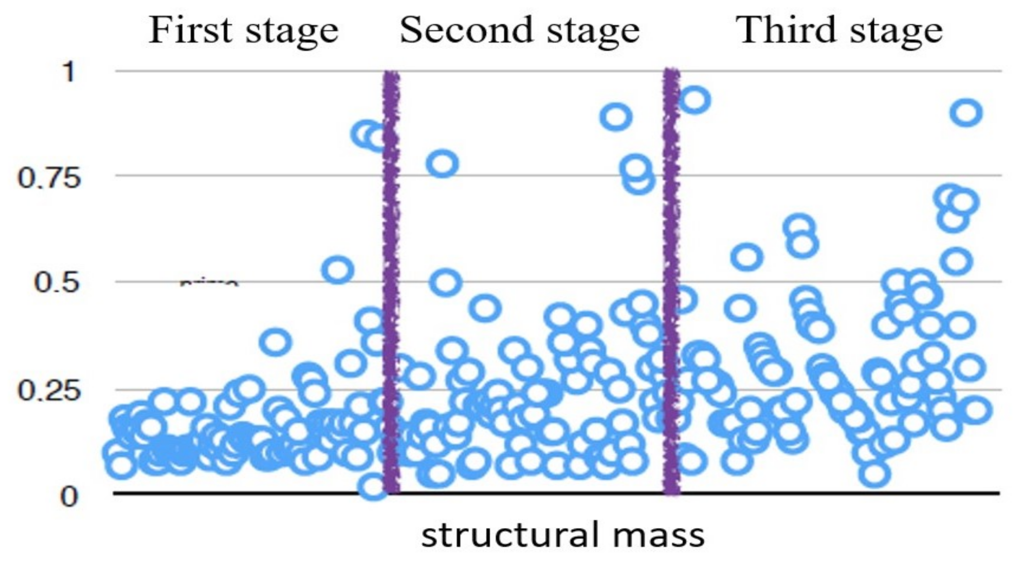
Other parameters defined by technical constraints are the structural mass ratio of each stage (1): Figure 3 shows these values for a number of stages taken from the database [18], and we have average values

$${ϵ}_1=0.11,{ϵ}_2=0.13,{ϵ}_3=0.3$$

(6)

It is important to know that if the total mass $M_1$, the payload mass $m_{pay}$ and the values ${ϵ}_k$, $Is{p}_k$ are given, there is an optimal selection of $U_k$, maximizing the Tziolkowski velocity (4). The procedure to identify the optimal subrocket mass ratios $U_k^{*}$ is in Appendix A.

The parameters ${ϵ}_k$, $Is{p}_k$ can be easily guessed at the first step of the rocket design, and the maximum payload mass $m_{pay}$ to be inserted into a specific reference orbit is the performance characterizing a space launcher.

With ${ϵ}_k$, $Is{p}_k$, and $m_{pay}$ fixed, the total mass $M_1$ determines the optimal mass distribution $U_k^{*}$ (staging) and the maximum Tziolkowski velocity, according to Appendix A. If this velocity is equal to the velocity required to inject the payload mass $m_{pay}$ into the reference orbit, $M_1$ is the launcher lift-off mass achieving this performance.

One point to underline is that the velocity to be provided by the thrust is not equal to the orbital velocity of a spacecraft on a circular orbit of altitude h: $V_a=\sqrt{\frac{\mu }{h+R_E}}$. In fact, we must consider the losses: these depend on each phase of the ascent trajectory. In the present Section it is assumed that the launcher velocity due to thrust must be overcome by 30% the required value for orbit injection. The orbit velocity relative to the Earth ${\overrightarrow{V}}_R$ depends on the latitude L of the launch site and on the azimuth $\psi$

$$V_R=\sqrt{V_a^2+V_E^2-2V_a{V}_{E}sin\psi }$$

where $V_E={\omega }_E{R}_{E}cos\left(L\right)$ is the velocity of the launch site and the azimuth angle $\psi$ is related to the launch site latitude and orbit inclination by the equation: $sin\psi =\frac{cosi}{cosL}$.

Then, the required velocity is here defined as

$$V_{req}=V_R(1+30\%)$$

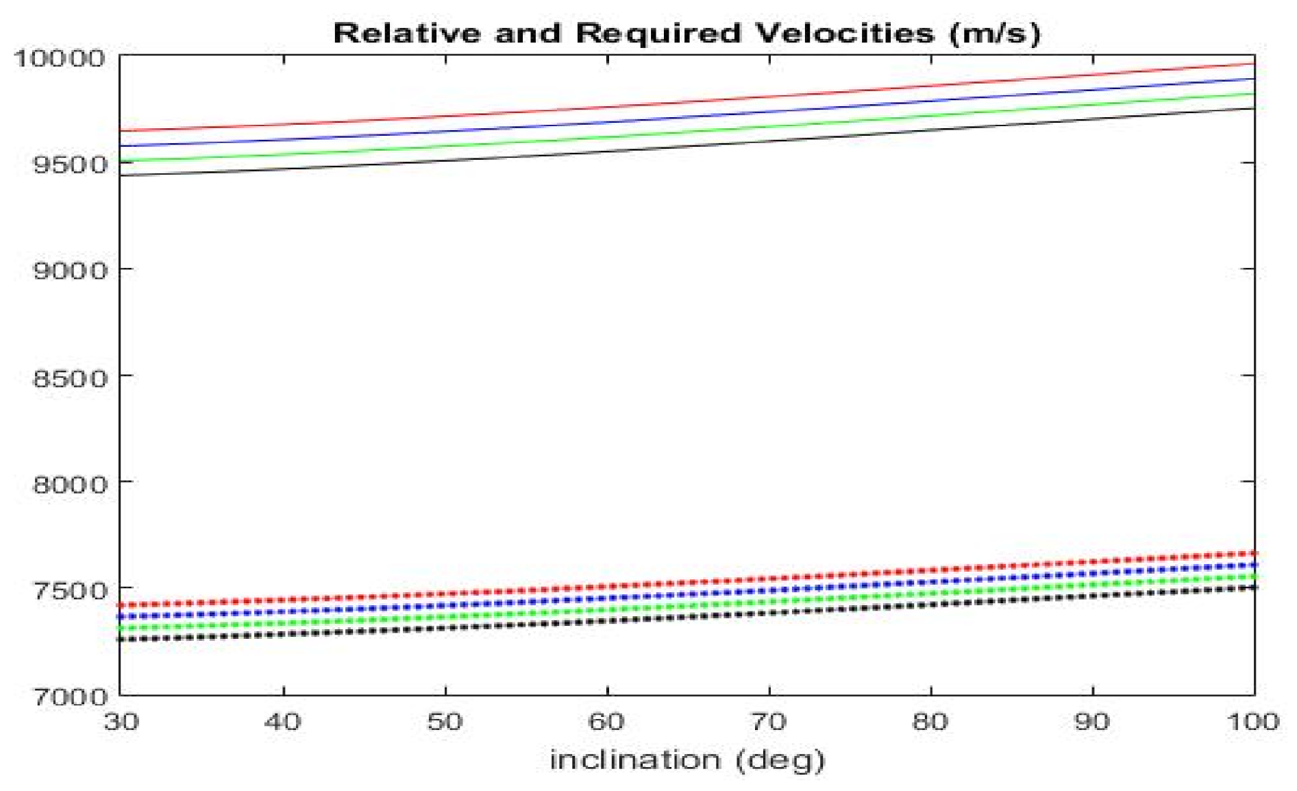
Figure 4 shows the relative (in blue) and required (in red) velocities to achieve a reference circular orbit of altitude h = 650 km with different inclinations from a launch site at L = 30 deg N.

Table 2. Minimumlift-off mass to inject the payload mass into circular polar orbit of altitude $h=650\mathrm{km}$ (average parameters (5) and (6), and launch site L = 30 deg).

Initial Mass ${\mathit{M}}_1$	Payload Mass ${\mathit{m}}_{\mathbf{pay}}$
18,000 kg	100 kg
36,000 kg	200 kg
54,000 kg	300 kg
72,000 kg	400 kg
90,000 kg	500 kg

shows the minimum mass at lift off for a micro-launcher having parameters (5) and (6) for different payload masses (from 100 to 1000 kg) to be injected into the reference orbit ($V_{req}=9805\mathrm{m}/\mathrm{s}$). The ratio $\frac{M_1}{m_{pay}}$ is constant.

3. A Second Step (Gravity Losses)

At lift off, the launcher performs a vertical trajectory followed by a pitch manoeuvre to select the required orbit plane. Then, to limit the aerodynamic loads on the structure, any launcher is forced to follow a zero angle of attack trajectory ($\alpha =0$) during the atmospheric flight. This trajectory is called the gravity-turn trajectory, and it is performed by the first stages of space launchers. The trajectory is basically planar and the state variables can be the relative velocity, flight-path angle, altitude and range $(V,\gamma ,h,s)$. The equations of motion are

$$\left\{\begin{array}{c}\dot{V}=\frac{T}{m}-\frac{\mu }{r^2}sin\gamma -\frac{1}{2}\rho V^2\frac{C_{D}S}{m}\hfill \\ \dot{\gamma }=\frac{\dot{s}}{R_E}-\frac{\mu }{r^{2}V}cos\gamma +\frac{1}{2}\rho V\frac{C_{L}S}{m}\hfill \\ \dot{h}=Vsin\gamma \hfill \\ \dot{s}=\frac{R_E}{r}Vcos\gamma \hfill \end{array}\right.$$

(7)

In fact, these equations are singular under the lift-off condition; $V=0,{\gamma }_0=\frac{pi}{2}$.

As observed in [14], this singularity generates an infinite number of solutions corresponding to the same lift-off condition: one can use this singularity to select among the different solutions the one with a prescribed final value, for instance a fixed flight-path angle ${\gamma }_f$ [15].

An analytic formula for the velocity V, due to Culler and Fried, was obtained under the following hypotheses:

• Constant gravity;
• Negligible drag and lift effect;
• Constant thrust-over-mass ratio $n=\frac{T}{gm}$.

The last of these is the strongest assumption, and is handled considering an average value $\overline{n}$ of the thrust-to-weight ratio. This average value can be computed using the formulas for the variation of mass $m=m_0-m_{d}t=m_0(1-qt)$ and the definition of the mass ratio $U=\frac{m_s}{m_0}$, which verifies $U=1-q{t}_b$.

Then

$$\begin{array}{ccc}\hfill \overline{n}& =& \frac{1}{t_b}{\int }_0^{tb}\frac{T}{mg}\left(t\right)dt=\frac{T}{g{t}_b{m}_0}{\int }_0^{tb}\frac{dt}{1-qt}=\hfill \\ & =& \frac{n_0}{t_b}\frac{1}{-q}{[ln(1-qt)]}_0^{t_b}=\frac{n_0}{-q{t}_b}ln(1-q{t}_b)=\hfill \\ & =& -\frac{n_0}{1-U}ln\left(U\right)=\frac{n_0}{1-U}ln\left(\frac{1}{U}\right)\hfill \end{array}$$

where $n_0=\frac{T}{g{m}_0}$ is the initial thrust-to-weight ratio.

Now two transformations are defined:

• From the flight-path angle variable $\gamma$ to the kick angle $\chi =\frac{\pi }{2}-\gamma$.
• From the kick angle $\chi$ to the variable $z=tan\frac{\chi }{2}$.

By the transformation in Equation (1) we have the following differential equations for the velocity and kick angle

$$\left\{\begin{array}{c}\dot{V}=-gcos\chi +g\overline{n}\hfill \\ \dot{\chi }=\frac{g}{V}sin\chi \hfill \end{array}\right.$$

(8)

Now the following trigonometrical equations are recalled

$$\begin{array}{ccc}\hfill cos\chi & =& \frac{1-{tan}^2\frac{\chi }{2}}{1+{tan}^2\frac{\chi }{2}}=\frac{1-z^2}{1+z^2}\hfill \\ \hfill sin\chi & =& sin\left(2\frac{\chi }{2}\right)=2sin\frac{\chi }{2}cos\frac{\chi }{2}=2tan\frac{\chi }{2}{cos}^2\frac{\chi }{2}=\frac{2z}{1+z^2}\hfill \end{array}$$

showing that the transformation to the z-variable allows us to transform the trigonometric function in rational functions. Then, Equation (8) becomes

$$\left\{\begin{array}{c}{\displaystyle \dot{V}=-g\overline{n}-g\frac{1-z^2}{1+z^2}}\hfill \\ {\displaystyle \dot{z}=\frac{g}{V}z}\hfill \end{array}\right.$$

(9)

Dividing the first by the second equation of the system (9), one has

$$\frac{dV}{dz}=\overline{n}\frac{V}{z}-\frac{V}{z}\frac{1-z^2}{1+z^2}$$

that is

$$\frac{dV}{V}=\left(\frac{\overline{n}}{z}-\frac{1}{z}\frac{1-z^2}{1+z^2}\right)dz$$

By integration

$$V=A{z}^{\overline{n}-1}(1+z^2)$$

(10)

The velocity in (10) is a function of the variable z. The time dependence can be obtained deriving the relation between time and z. Substitution of (10) in the second equation of the system (9) gives

$$\dot{z}=\frac{dz}{dt}=-\frac{g}{A}\frac{1}{z^{\overline{n}-2}(1+z^2)}$$

by separation of variables and integrating from $t_0=0$ to t

$$t=\frac{A}{g}\left(\frac{z^{\overline{n}-1}}{\overline{n}-1}+\frac{z^{\overline{n}+1}}{\overline{n}+1}\right)$$

(11)

The launch initial conditions are in the given hypothesis

$$\left\{\begin{array}{c}{V}_0=0\hfill \\ {\gamma }_0=\frac{\pi }{2}\hfill \\ {\chi }_0=0\Rightarrow z_0=0\hfill \end{array}\right.$$

Imposing these initial conditions in the solution (10), one has

$$V_0=A{z}_0^{\overline{n}-1}(1+z_0^2)=0\forall A$$

Then, the initial conditions are verified for any value of the constant A. That is, there are infinite (gravity-turn) solutions for the velocity, parameterized by A, corresponding to the same initial condition. This violation of the Chauchy theorem on uniqueness of the solution of a differential equation is due to the singularity of $\dot{z}$ for $V=0$ in the system (9).

One can take advantage of this multiplicity of solutions to select for instance the solution that achieves a chosen flight-path angle ${\gamma }_f$ at the burn-out time $t_b$. The chosen ${\gamma }_f$ defines a value $z_f=\tan \left(\frac{\pi /2-{\gamma }_f}{2}\right)$. By Equation (11), one obtains

$$A=g{t}_b{\left(\frac{z_f^{\overline{n}-1}}{\overline{n}-1}+\frac{z_f^{\overline{n}+1}}{\overline{n}+1}\right)}^{-1}$$

(12)

and the related velocity is obtained inserting this value of A into Equation (10).

In particular, the velocity at burn out is

$$V_f=A{z}_f^{\overline{n}-1}(1+z_f^2)$$

(13)

In addition, the altitude h and range s can be easily derived [16]. For the altitude

$$\dot{h}=Vsin\gamma =Vcos\chi =V\frac{1-z^2}{1+z^2}$$

Then

$$\frac{dh}{dz}=\frac{\dot{h}}{\dot{z}}=\frac{V^2}{gz}\frac{1-z^2}{1+z^2}$$

By Equation (10), one has

$$\frac{dh}{dz}=\frac{A^2}{g}\left(z^{2\overline{n}-3}-z^{2\overline{n}+1}\right)$$

The elementary integration of the above equation between current z and initial $z_0$ gives the formula for the altitude

$$h\left(z\right)=h\left(z_0\right)+\frac{A^2}{g}{\left[\frac{z^{2\overline{n}-2}}{2\overline{n}-2}-\frac{z^{2\overline{n}+2}}{\overline{n}+2}\right]}_{z_0}^{z_f}$$

(14)

For the range s

$$\dot{s}=Vcos\gamma =V\sin \chi =2V\frac{z}{1+z^2}$$

then

$$\frac{ds}{dz}=\frac{\dot{s}}{\dot{z}}=2\frac{A^2}{g}\left(z^{2\overline{n}-1}+z^{2\overline{n}+1}\right)$$

The integration gives the formula for the range

$$s\left(z\right)=s\left(z_0\right)+2\frac{A^2}{g}{\left[\frac{z^{2\overline{n}}}{2\overline{n}}+\frac{z^{2\overline{n}+2}}{2\overline{n}+2}\right]}_{z_0}^{z_f}$$

(15)

Equations (10), (12), (14) and (15), together with (11), provide the state variables of the gravity-turn trajectory of a single-stage rocket with flight-path angle ${\gamma }_f$ at burn-out time $t_b$.

For instance, let us consider initial lift off condition $(V_0=0,{\chi }_0=0,h_0=0,s_0=0)$ and choose the final condition ${\gamma }_f=0$ this condition corresponds to $z_f=1$. Then Equation (12) gives

$$A=g{t}_b\frac{{\overline{n}}^2-1}{2\overline{n}}$$

By Equations (10), (14) and (15), the velocity, altitude and range at burn out are equal to

$$V_f=2A=g{t}_b\frac{{\overline{n}}^2-1}{\overline{n}}$$

(16)

$$h_f=\frac{A^2}{g}\frac{1}{\overline{n}-1}=\frac{g{t}_b^2}{2}\frac{{\overline{n}}^2-1}{{\overline{n}}^2}$$

$$s_f=\frac{A^2}{g}\left(\frac{1}{\overline{n}}+\frac{1}{\overline{n}+1}\right)=\frac{g{t}_b^2}{2}{\left(\frac{{\overline{n}}^2-1}{\overline{n}}\right)}^2\left[\frac{1}{2\overline{n}}+\frac{1}{2\overline{n}+2}\right]$$

Note that the final velocity formula of a rocket is generally obtained by the Tziolkowski formula that takes into account only the thrust acceleration. In the present setting, the Tziolkowski formula gives the final velocity

$$V_{Tz}=g\overline{n}{t}_b$$

The final velocity obtained here, which includes gravity effect, is given by (16): the difference among the two is the gravity loss and it is equal to

$$\Delta V_g=V_{Tz}-V_f=\frac{g{t}_b}{\overline{n}}$$

(17)

The above results can be generalized to multistage launchers.

4. Analytic Derivation of Launcher Trajectories

The above analytic formulas can be generalized to multistage launchers. Let us start with two stages with the following average parameters ($n_1,Is{p}_1,u_1$) and ($n_2,Is{p}_2,u_2$).

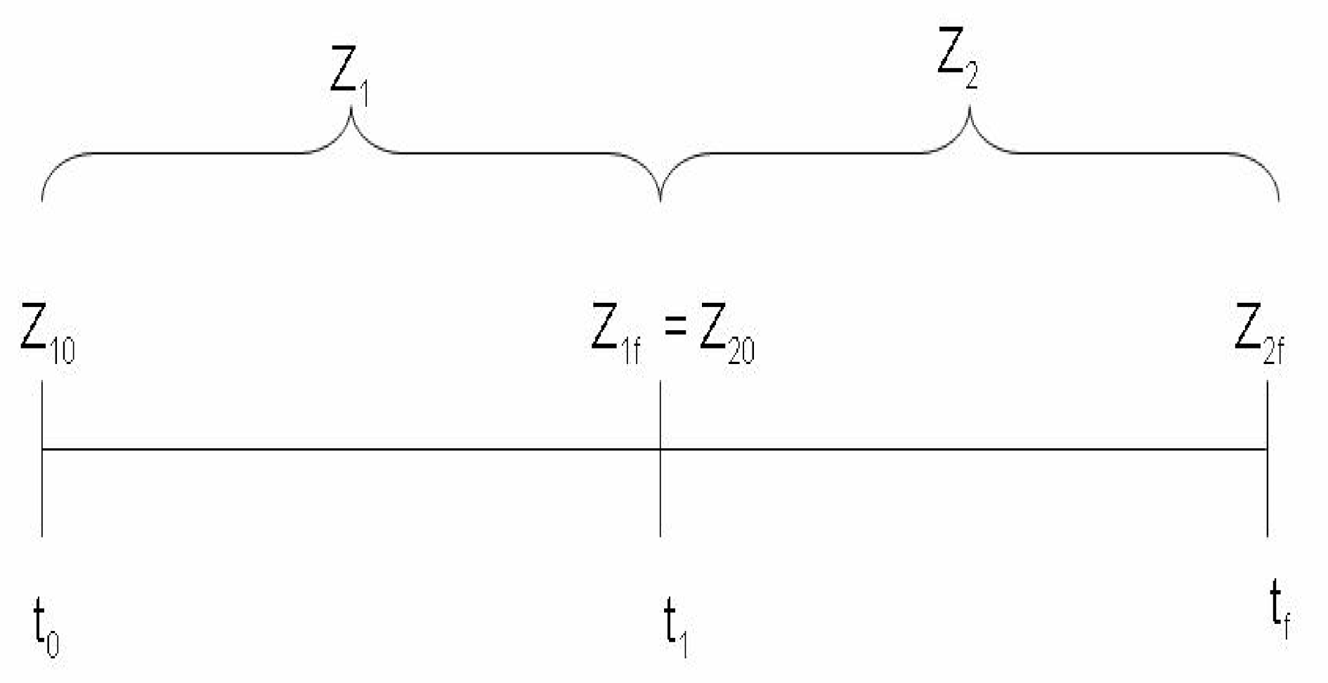
The first stage has variables $z_1$, $V_1=A_1{z}_1^{{\overline{n}}_1-1}(1+z_1^2)$ in the time interval $[t_{10}=0,t_{1f}=t_{b_1}]$. The second stage has variables $z_2$, $V_2=A_2{z}_2^{{\overline{n}}_2-1}(1+z_2^2)$ in the time interval $[t_{20}=t_{b_1},t_{2f}=t_{b_2}+t_{b_1}]$ and the final value $z_{2_f}$ is fixed (see Figure 5).

Of course the two solutions $z_1,V_1$ and $z_2,V_2$ must match at the boundary point

$$z_{1f}=z_{20}$$

$$V_{1f}=V_1\left(z_{1f}\right)=V_2\left(z_{20}\right)=V_{20}$$

The two matching conditions imply

$$\frac{A_1}{A_2}=z_{20}^{{\overline{n}}_2-{\overline{n}}_1}$$

(18)

Equation (11) gives at first-stage burn out

$$t_{b1}=\frac{A_1}{g}\left(\frac{z_{20}^{{\overline{n}}_1-1}}{{\overline{n}}_1-1}+\frac{z_{20}^{{\overline{n}}_1+1}}{{\overline{n}}_1+1}\right){=}^{def}{f}_1\left(z_{20}\right)$$

(19)

At the burn out of the second stage, one has $z_{2f}$ and

$$t_{b2}=\frac{A_2}{g}\left(\frac{z_{2f}^{{\overline{n}}_2-1}}{{\overline{n}}_2-1}+\frac{z_{2f}^{{\overline{n}}_2+1}}{{\overline{n}}_1+1}-\frac{z_{20}^{{\overline{n}}_2-1}}{{\overline{n}}_2-1}+\frac{z_{20}^{{\overline{n}}_2+1}}{{\overline{n}}_1+1}\right){=}^{def}{f}_2\left(z_{20}\right)$$

(20)

We have a system of three Equations (18)–(20) in the three unknowns $A_1$, $A_2$ and $z_{20}$.

To solve it, let us consider the ratio

$$\frac{t_{b2}}{t_{b1}}=\frac{f_1}{f_2}$$

Because of (18), this ratio is a function of $z_{20}$ only

$$f\left(z_{20}\right)=\frac{t_{b2}}{t_{b1}}-\frac{f_1}{f_2}=0$$

The solution $z_{20}$ of $f\left(z_{20}\right)=0$ (in the range [0,1]) provides the value of the flight-path angle at the end of the first stage. Moreover, by Equation (20), one finds $A_2$ and by Equation (19) one finds $A_1$. Hence, the velocity profile of the two-stage launcher with a prescribed flight-path angle $z_{2f}$ at second-stage burn out is equal to

$$\begin{array}{c}V\left(z\right)=A_1{z}_1^{{\overline{n}}_1-1}(1+z_1^2)forz\in [0,z_{20}]\hfill \\ V\left(z\right)=A_2{z}_2^{{\overline{n}}_2-1}(1+z_2^2)forz\in [z_{20},z_{2f}]\hfill \end{array}$$

(21)

With same arguments, we obtain the altitude and range

$$\begin{array}{c}{\displaystyle h\left(z\right)=\frac{A_1^2}{g}\left[\frac{z_1^{2{\overline{n}}_1-2}}{2{\overline{n}}_1-2}-\frac{z_1^{2{\overline{n}}_1+2}}{{\overline{n}}_1+2}\right],forz\in [0,z_{20}]}\hfill \\ {\displaystyle h\left(z\right)=h\left(z_{20}\right)+\frac{A_2^2}{g}{\left[\frac{z_2^{2{\overline{n}}_2-2}}{2{\overline{n}}_2-2}-\frac{z_2^{2{\overline{n}}_2+2}}{{\overline{n}}_2+2}\right]}_{z_{20}}^z,forz\in [z_{20},z_{2f}]}\hfill \end{array}$$

(22)

$$\begin{array}{c}{\displaystyle s\left(z\right)=2\frac{A_1^2}{g}\left[\frac{z^{2{\overline{n}}_1}}{2{\overline{n}}_1}+\frac{z^{2{\overline{n}}_1+2}}{2{\overline{n}}_1+2}\right],forz\in [0,z_{20}]}\hfill \\ {\displaystyle s\left(z\right)=R\left(z_{20}\right)+2\frac{A_2^2}{g}{\left[\frac{z^{2{\overline{n}}_2}}{2{\overline{n}}_2}+\frac{z^{2{\overline{n}}_2+2}}{2{\overline{n}}_2+2}\right]}_{z_{20}}^z,forz\in [z_{20},z_{2f}]}\hfill \end{array}$$

(23)

Note that the gravity loss of the two-stage launcher is

$$\Delta V_g=gIs{p}_{1}log\left(\frac{1}{U_1}\right)+gIs{p}_{2}log\left(\frac{1}{U_2}\right)-V\left(z_{2f}\right)$$

Any number of stage N can be handled: of course, more numerical work is needed to find out the unknown variables. The N-1-matching conditions on the flight-path angle generate the following N-1-matching conditions on the velocity

$$\begin{array}{ccc}\hfill V_1(z_{20},A_1)& =& V_2(z_{20},A_2)\hfill \\ \hfill V_2(z_{30},A_2)& =& V_3(z_{30},A_3)\hfill \\ & ⋮& \\ \hfill V_{N-2}(z_{N-20},A_{N-2})& =& V_{N-1}(z_{N-10},A_{N-1})\hfill \end{array}$$

These, together with the N relationships related to each burn time

$$\begin{array}{ccc}\hfill t_{b_1}& =& t_{b_1}(A_1,z_{20})\hfill \\ \hfill t_{b_2}& =& t_{b_2}(A_2,z_{20},z_{30})\hfill \\ & ⋮& \\ \hfill t_{b_N}& =& t_{b_N}(A_N,z_{20},\cdots ,z_{N0})\hfill \end{array}$$

generate $2N-1$ equations to be solved with respect to the $2N-1$ unknowns $z_{20},z_{30},\cdots z_{N0}$, $A_1,\cdots A_N$.

By these solutions, the velocity, altitude and range profiles can be computed using Equations (13)–(15) in the ranges $[0,z_{20}],\cdots [z_{N0},z_f]$.

For instance, for a three-stage launcher, one has

$$t_{b1}=\frac{A_1}{g}\left(\frac{z_{20}^{n_1-1}}{n_1-1}+\frac{z_{20}^{n_1+1}}{n_1+1}\right)$$

(24)

$$t_{b2}=\frac{A_2}{g}\left[\left(\frac{z_{30}^{n_2-1}}{n_2-1}+\frac{z_{30}^{n_2+1}}{n_2+1}\right)-\left(\frac{z_{20}^{n_2-1}}{n_2-1}+\frac{z_{20}^{n_2+1}}{n_2+1}\right)\right]$$

(25)

$$t_{b3}=\frac{A_3}{g}{\left[\left(\frac{z_3^{n_3-1}}{n_3-1}+\frac{z_3^{n_3+1}}{n_3+1}\right)\right]}_{z_{3_0}}^{z_{3_f}}$$

(26)

$$A_1=A_2{z}_{20}^{{\overline{n}}_2-{\overline{n}}_1}$$

(27)

$$A_2=A_3{z}_{30}^{{\overline{n}}_3-{\overline{n}}_2}$$

(28)

(these five Equations (24)–(28) with the five unknowns $A1$, $A_2$, $A_3$, $z_{20}$, $z_{30}$).

One solution is to write the variables $A_1$ and $A_2$ as function of $A_3$ using Equations (27) and (28). Then, the ratios $\frac{t_{b_2}}{t_{b_1}}$, $\frac{t_{b_3}}{t_{b_1}}$ are obtained dividing (25) and (26) by the Equation (24). The two ratios give two equations on the two unknown $z_{20}$, $z_{30}$. The solutions can be found numerically within the interval [0,1], and they determine the values of the flight-path angles at the end of the first and second stages. The values $A_1$, $A_2$, $A_3$ are derived by Equations (24) and (26) and and the velocities at the end of each stage are obtained.

For a four-stage launcher, there are seven equations in the seven unknowns $A1$, $A_2$, $A_3$, $A_4$, $z_{20}$, $z_{30}$, $z_{40}$

$$A_1=A_2{z}_{20}^{{\overline{n}}_2-{\overline{n}}_1}$$

(29)

$$A_2=A_3{z}_{30}^{{\overline{n}}_3-{\overline{n}}_2}$$

(30)

$$A_3=A_4{z}_{40}^{{\overline{n}}_4-{\overline{n}}_3}$$

(31)

$$t_{b1}=\frac{A_1}{g}\left(\frac{z_{20}^{n_1-1}}{n_1-1}+\frac{z_{20}^{n_1+1}}{n_1+1}\right)$$

(32)

$$t_{b2}=\frac{A_2}{g}\left[\left(\frac{z_{30}^{n_2-1}}{n_2-1}+\frac{z_{30}^{n_2+1}}{n_2+1}\right)-\left(\frac{z_{20}^{n_2-1}}{n_2-1}+\frac{z_{20}^{n_2+1}}{n_2+1}\right)\right]$$

(33)

$$t_{b_3}=\frac{A_3}{g}\left[\left(\frac{z_{40}^{n_3-1}}{n_3-1}+\frac{z_{40}^{n_3+1}}{n_3+1}\right)-\left(\frac{z_{30}^{n_3-1}}{n_3-1}+\frac{z_{30}^{n_3+1}}{n_3+1}\right)\right]$$

(34)

$$t_{b_4}=\frac{A_4}{g}\left[\frac{2n_4}{n_4^2-1}-\left(\frac{z_{40}^{n_4-1}}{n_4-1}+\frac{z_{40}^{n_4+1}}{n_4+1}\right)\right]$$

(35)

The first three equations allow us to write $A_1$, $A_2$, $A_3$ as function of $A_4$ only. Then, the three ratios $\frac{t_{b_2}}{t_{b_1}}$, $\frac{t_{b_3}}{t_{b_1}}$, $\frac{t_{b_4}}{t_{b_1}}$ are functions of the three unknowns $z_{20}$, $z_{30}$, $z_{40}$. The solution is used then to derive $A_1-A_4$.

Note that the above formulas for three- or four-stage launchers provide the values of the flight-path angles and the velocities at the end of each stage for the launcher trajectory with a fixed value of the final flight-path angle.

5. Guidance

The gravity-turn trajectory constrains the guidance and should be abandoned if possible; the relevant condition is the factor $q\alpha$, where $q=\frac{1}{2}\rho V^2$ is the dynamical pressure and $\alpha$ is the angle of attack. This factor must be below a limit ${\left[q\alpha \right]}_{max}$ which is peculiar to any launcher and can be satisfied by the gravity-turn ($\alpha =0$) trajectory. As the altitude increases, the atmospheric density $\rho$ decreases exponentially, so at a certain point of the flight the condition of $q\alpha$ disappears and a different guidance can be applied. The guidance applied here is based on: (A) a possible coasting arc, and (B) thrust along the horizontal direction.

Generally, a coasting arc is performed after the burn out of the stage $N-1$ of an N stage launcher to increase the altitude at the cost of a moderate decrease in velocity. After the coasting arc, the launcher is close to the target altitude $h_f$, whereas the required velocity $V_{req}$ must be gained. This velocity basically has the horizontal direction $\widehat{\theta }=cos\gamma \widehat{V}+sin\gamma \widehat{l}$, then the thrust direction is along $\widehat{\theta }$ during the N-stage boost.

With the above guidance scheme, the full launcher trajectory depends on two parameters: the flight-path angle ${\gamma }_f$ at the end of the gravity-turn phase and the duration $t_c$ of the coasting arc. The two parameters $({\gamma }_f,t_c)$ are introduced into an iterative routine (such as the Matlab routine fsolve.m) and updated to set the errors on the final altitude and velocity $(h\left(t_b\right)-h_f,V\left(t_b\right)-V_{req})$ to zero, where $t_b$ is the N-stage burn-out time.

Let us consider a three-stage rocket as an example. The first two stages are in gravity turn with a prescribed final flight-path angle ${{\gamma }_2}_f$, then a costing arc of duration $t_c$ is performed. Finally the third-stage boost is applied with horizontal thrust direction. The Matlab routine fsolve.m is used to update the values $({{\gamma }_2}_f,t_c)$, for instance, to achieve the polar circular orbit of altitude $h_f=650$ km from a launch site with a latitude of 30 deg N. The required velocity is then equal to $V_R=7542$ m/s.

The launcher has the parameters reported in

Table 3. Dataof the three-stage launcher.

Total mass $M1$	55,500 kg
Payload mass $m_{pay}$	405 kg
${ϵ}_1$, ${ϵ}_2$, ${ϵ}_3$	0.10, 0.11, 0.22
$Is{p}_1$, $Is{p}_2$, $Is{p}_3$	294  s, 295  s, 300  s
$U_1$, $U_2$, $U_3$	0.35, 0.32, 0.31
${n_0}_1$, ${n_0}_2$, ${n_0}_3$	2.40, 2.06, 2.32
${\overline{n}}_1$, ${\overline{n}}_2$, ${\overline{n}}_3$	3.85, 3.45, 3.95

. The Tziolkowski velocity is equal to $\Delta V_{Tz}=9743\mathrm{m}/\mathrm{s}$. From the data of Table 3 it is possible to derive the mass parameters of each stage $m_{s_1},m_{p_1}$, $m_{s_2},m_{p_2}$, $m_{s_3},m_{p_3}$ and the mass of each substage $M_2,M_3$, see Equations (A1) and (A2) in Appendix A. From the values $n_{0_1}$, $n_{0_2}$, $n_{0_3}$ and $M_1$, $M_2$, $M_3$, it is possible to derive the propellant mass rates ${\dot{m}}_1$, ${\dot{m}}_2$, ${\dot{m}}_3$, hence the burn times $t_{b_i}=\frac{m_{p_i}}{{\dot{m}}_i},i=1,3$. For any fixed ${\gamma }_{2_f}$, the Equations (21)–(23) give the state of the launcher at the end of the second stage where the gravity-turn phase ends. After a coasting of duration $t_c$, the third stages thrust the rocket up to the burn time $t_{b_3}$; the final altitude and velocity are compared with the required $(h_f,V_R)$. The parameters ${\gamma }_{2_f}$, $t_c$ are updated in order to match the required final orbit conditions. After few iterations, the routine finds the following parameters to reach the required orbit: ${{\gamma }_2}_f=26.5\mathrm{deg}$, $t_c=340\mathrm{s}$.

6. Numerical Comparison

The results obtained by the analytic formulas are now compared with a numerical code simulating the launcher trajectory with better accuracy. The equations of motion are the three-dimensional equations of flight in the relative velocity frame with state variables $(r,\lambda ,L,V_R,{\gamma }_R,{\psi }_R)$

$$\begin{array}{c}{\displaystyle \dot{r}=V_{R}sin{\gamma }_R}\hfill \\ \dot{\lambda }=V_{R}cos{\gamma }_R\frac{cos{\psi }_R}{rcosL}\hfill \\ \dot{L}=\frac{V_{R}cos{\gamma }_{R}sin{\psi }_R}{r}\hfill \\ {\dot{V}}_R=r{\omega }_E^{2}cosL(cosLsin{\gamma }_R-sinLcos{\gamma }_{R}sin{\psi }_R)+\frac{f_V}{m}\hfill \\ \begin{array}{c}\hfill {\dot{\gamma }}_R=\frac{V_R}{r}cos{\gamma }_R+2{\omega }_{E}cosLcos{\psi }_R+\\ \hfill +r\frac{{\omega }_E^2}{V_R}cosL(cosLcos{\gamma }_R+sinLsin{\gamma }_{R}sin{\psi }_R)+\frac{f_l}{mV}\end{array}\hfill \\ \begin{array}{c}\hfill {\dot{\psi }}_R=-\frac{V_R}{r}tanLcos{\gamma }_{R}cos{\psi }_R+2{\omega }_{E}cosLtan{\gamma }_{R}sin{\psi }_R+\\ \hfill -r\frac{{\omega }_E^2}{V_{R}cos{\gamma }_R}cosLsinLcos{\psi }_R-2{\omega }_{E}sinL\end{array}\hfill \end{array}$$

(36)

with

$$\begin{array}{c}{\displaystyle \frac{f_V}{m}=\frac{T}{m}cos\alpha -\frac{\mu }{r^2}sin{\gamma }_R-\frac{1}{2}\rho C_D\frac{S}{m}{V}_R^2}\hfill \\ .\hfill \\ {\displaystyle \frac{f_l}{m}=\frac{T}{mV}sin\alpha -\frac{\mu }{V_R{r}^2}cos{\gamma }_R+\frac{1}{2}\rho C_L\frac{S}{m}{V}_R}\hfill \end{array}$$

(37)

Equations (36) and (37) are used with $\alpha =0$ for the gravity-turn arc, with $T=0$ for the coasting arc and with $\alpha =\gamma$ for the third-stage boost. Lift off begins with an initial vertical arc of small duration $t_V$; this is computed in the Cartesian frame with non-singular coordinates. After the vertical arc, to turn the trajectory from the vertical direction, a pitch manoeuvre starts with a fixed direction of thrust $\alpha ={\theta }_k$ and ends when ${\gamma }_R={\theta }_k$. At this time (called pitch over), the gravity-turn trajectory starts. The pitch direction of thrust ${\theta }_k$ is chosen so to have the prescribed value ${\gamma }_{2_f}$ at the second-stage burn out. Then, the coasting arc duration is chosen to achieve the required orbit.

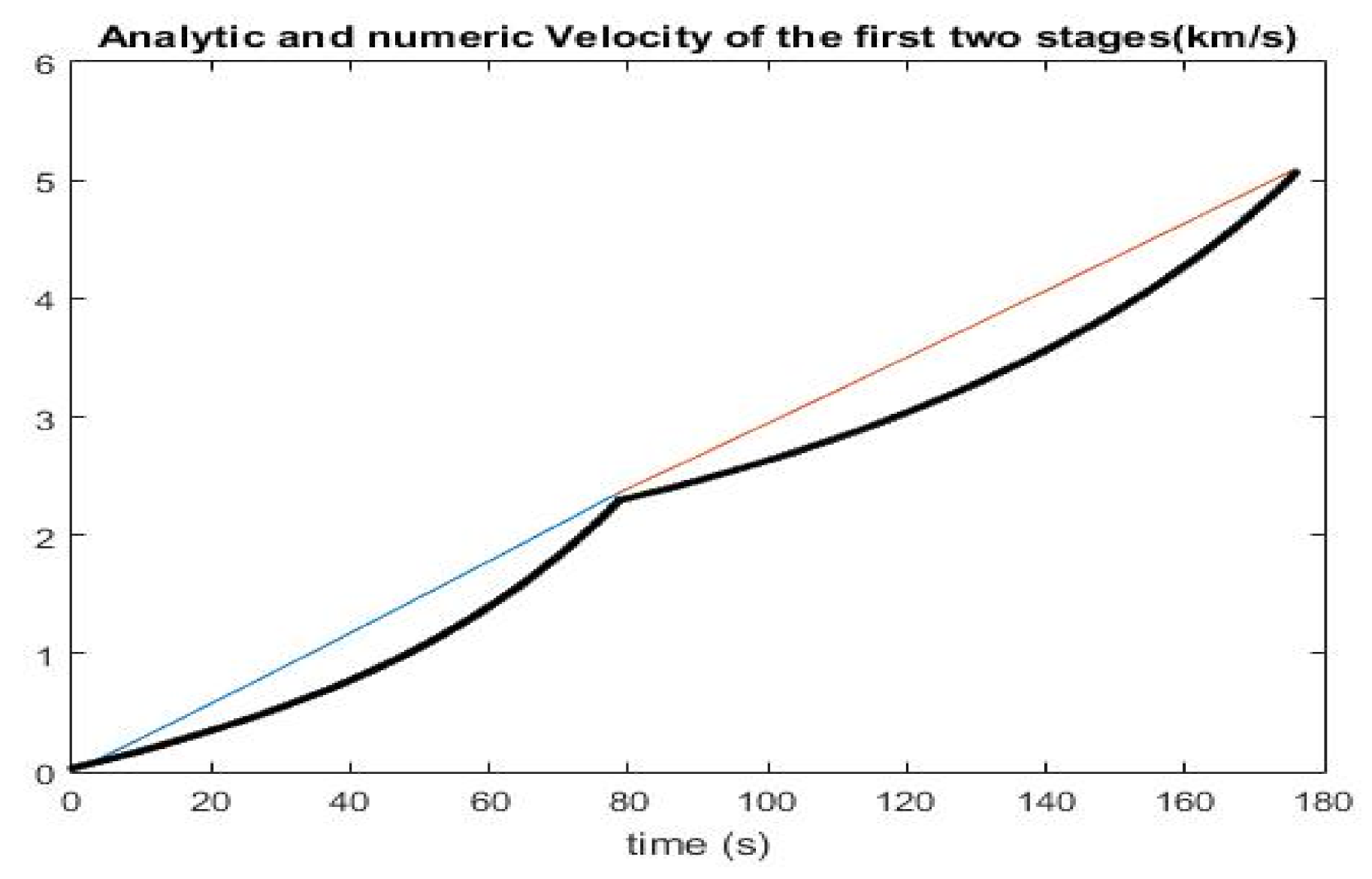
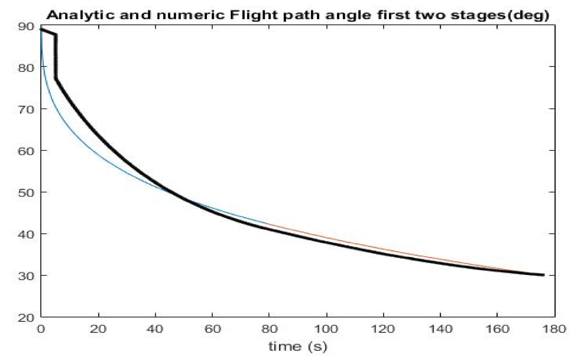
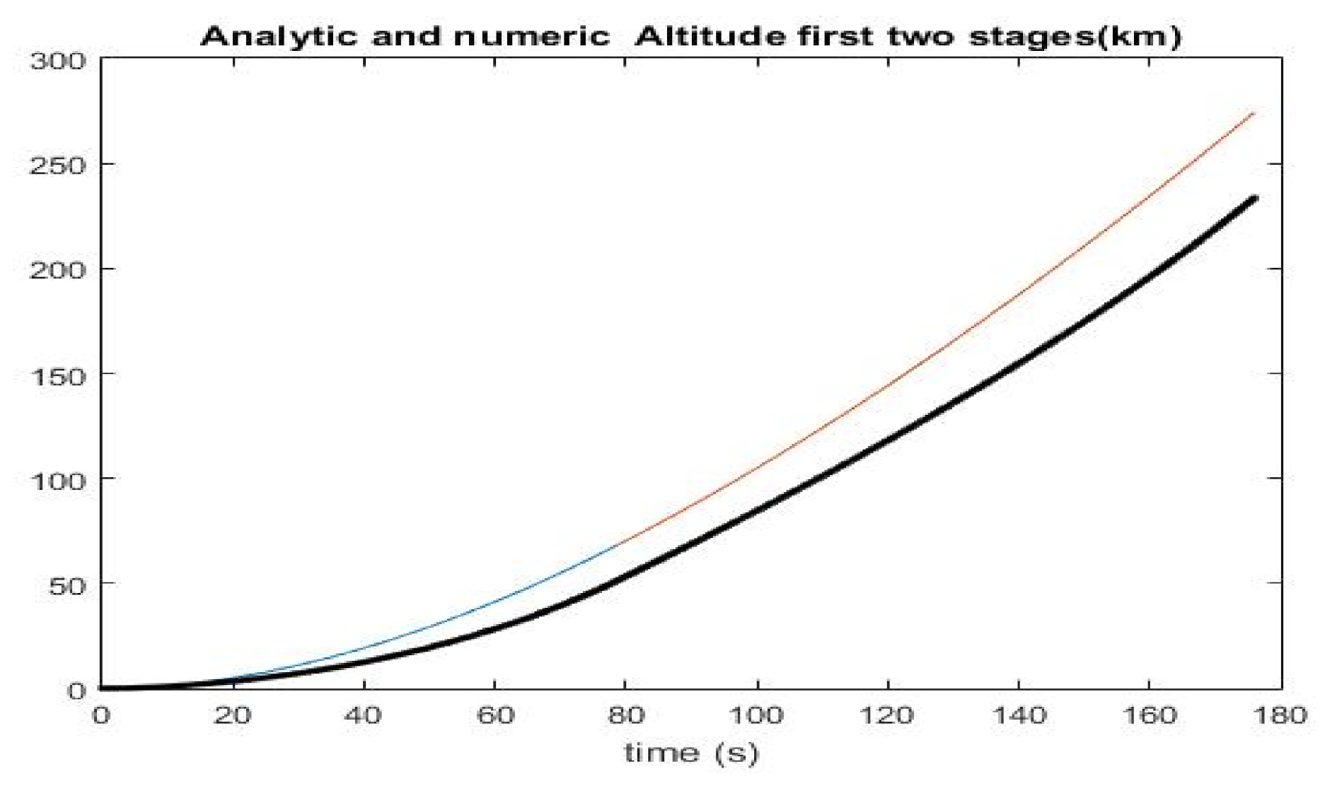
Figure 6, Figure 7 and Figure 8 show the analytical and numerical graphs of the velocity, flight-path angle and altitude during gravity turn. Note that at the end of the second stage the discrepancy between analytic and numeric results is rather small for the velocity, whereas a reduction of $15\%$ occurs in the altitude due to the numerical integration of the drag force. In the numerical calculation the atmospheric density is represented by the USATMO 76 model and the drag coefficient is kept constant at an average value $C_D=0.4$. The reference surface is $S=\frac{\pi d^2}{4}$, with a diameter of $d=2$ m. The drag effect reduces the payload mass that can be inserted into the reference orbit.

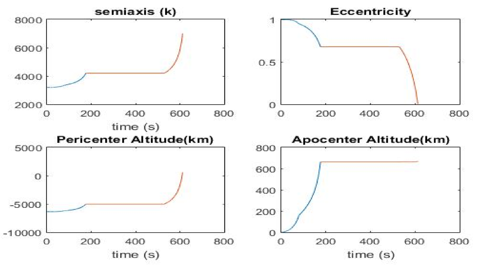
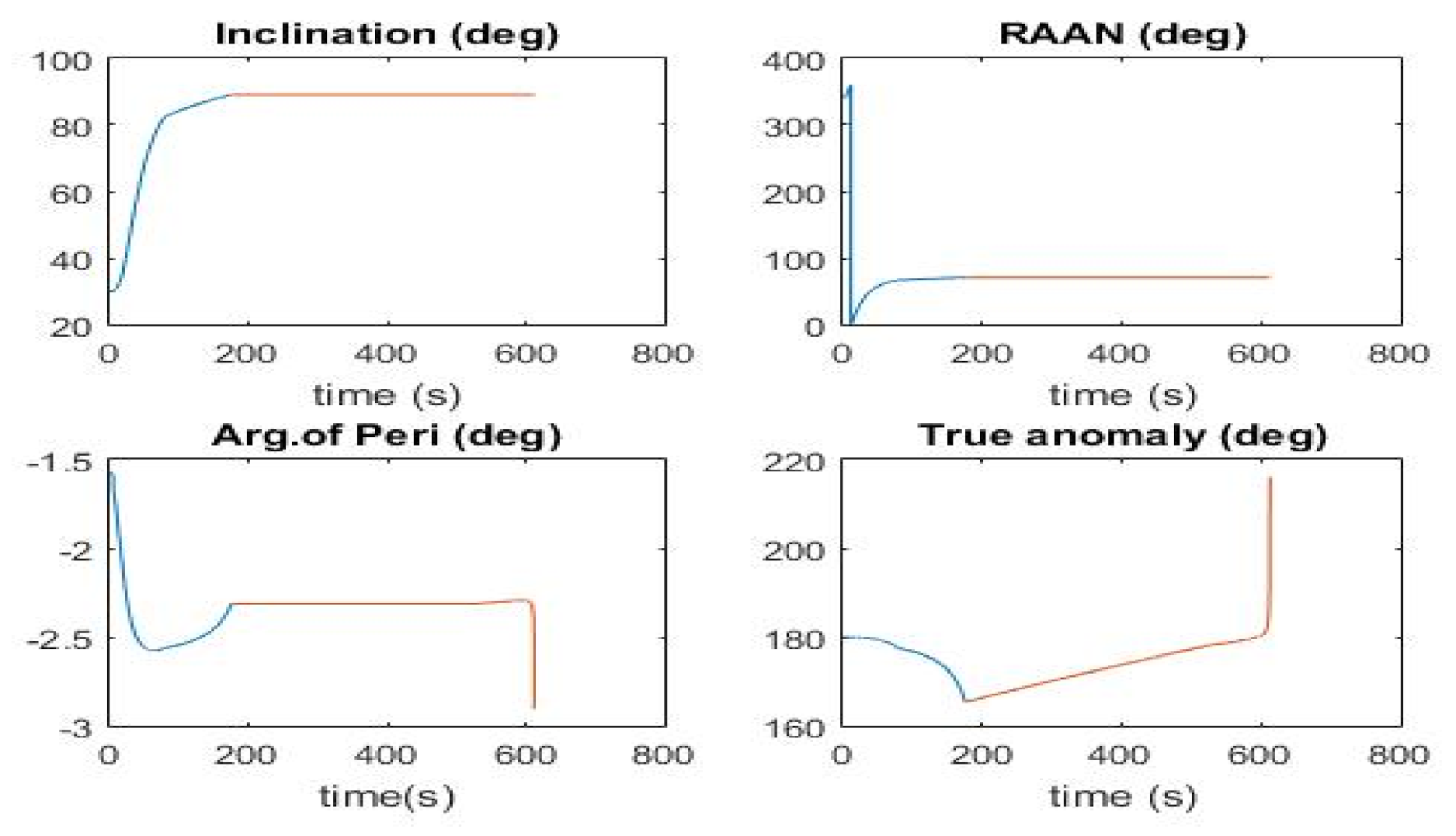
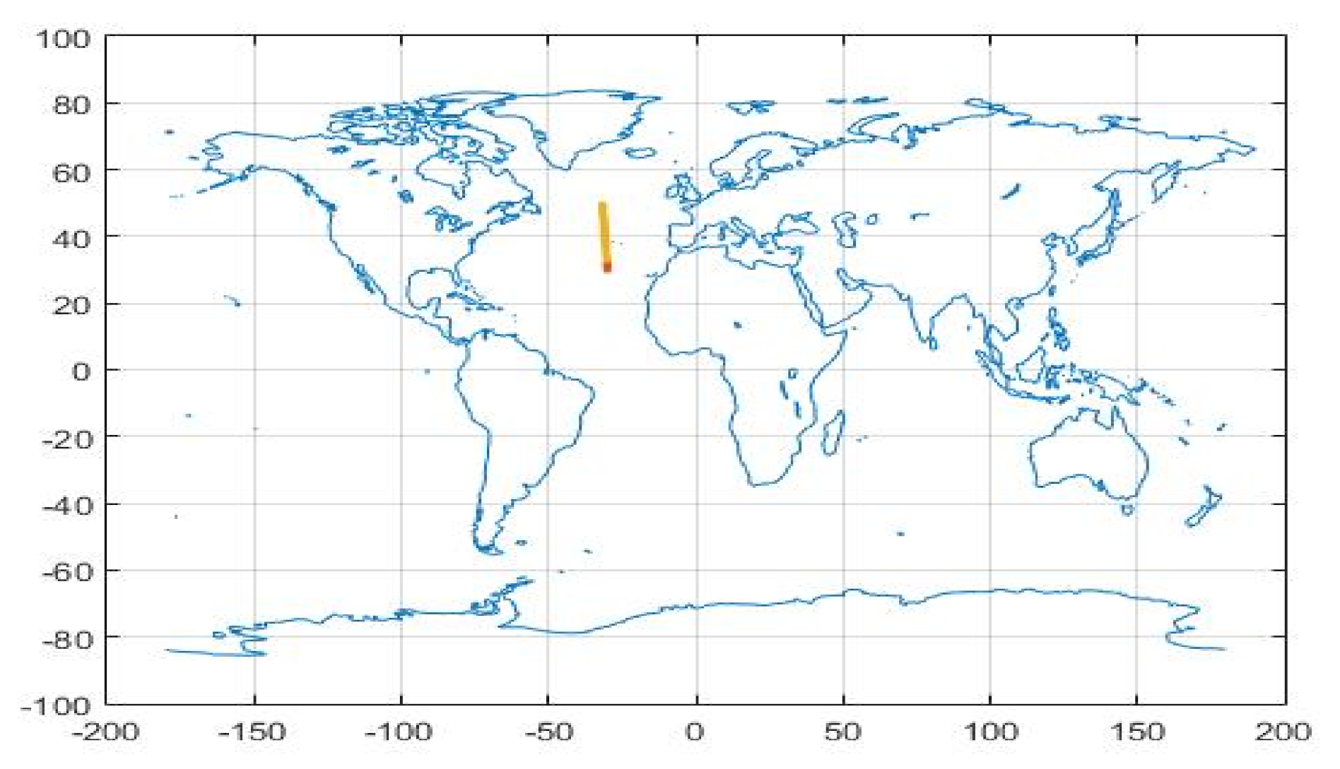
In fact, the numerical results give insertion in the polar circular orbit of altitude 650 km of a payload of mass $m_{pay}=390$ kg, vertical flight duration $t_v=5$ s, and pitch angle ${\theta }_k=76$ deg (generating ${\gamma }_{2_f}$ = $26.5$ deg), and coasting time $t_c=355$ s. The payload mass reduction with respect to the analytical results is about $4\%$. The evolution of the orbit parameters during the launch is shown in Figure 9 and Figure 10, and Figure 11 shows the launcher ground track.

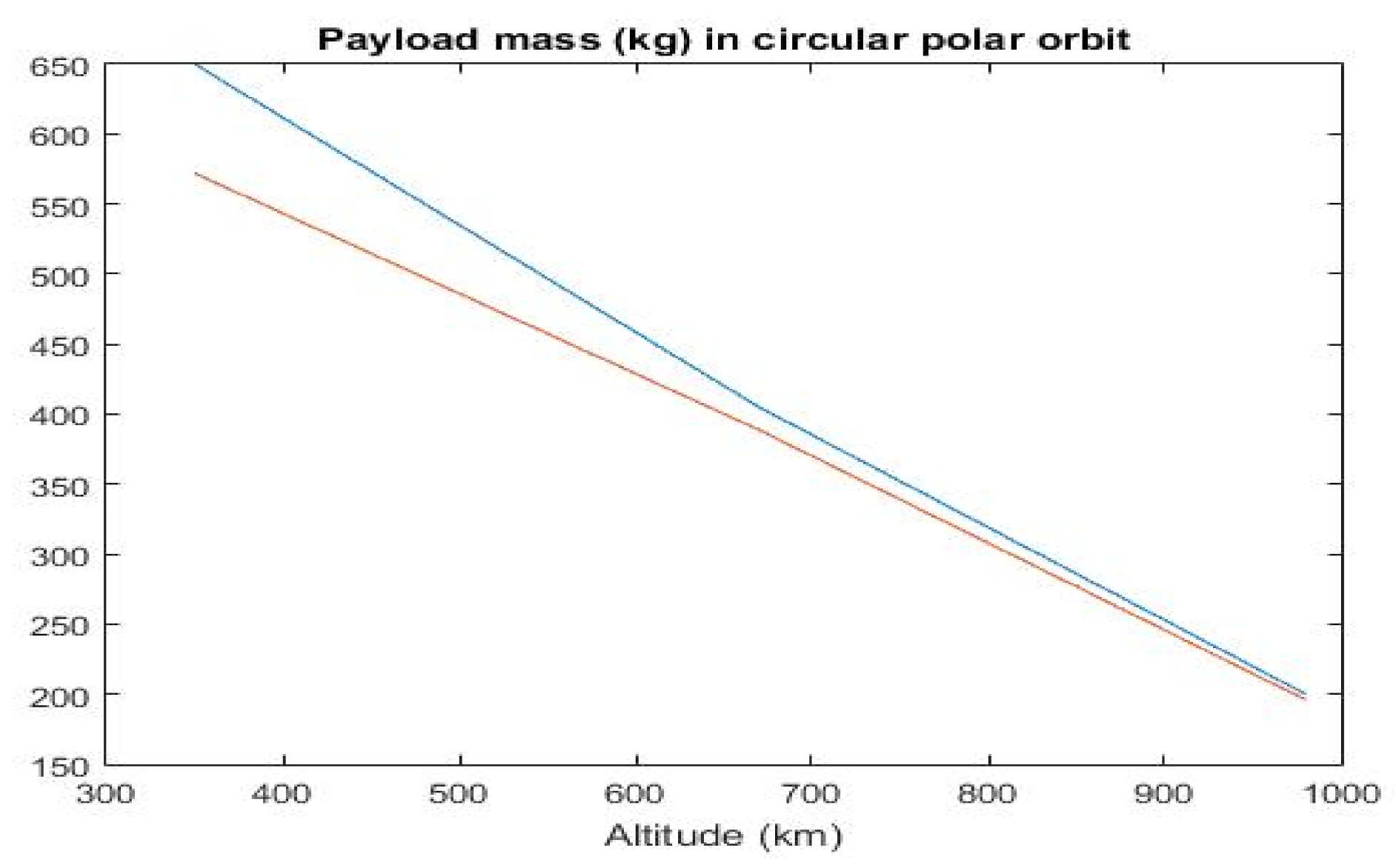
Figure 12 shows the payload mass evaluation for polar circular orbits of different altitudes obtained by the analytic (blue curve) and numerical (orange curve) algorithms. Of course, the bigger differences are for orbits of lower altitude; however, the reduction in the payload mass does not exceed $10\%$ of the value found analytically.

7. Concluding Remarks

This research extends the preceding generalization of the Culler and Fried formulation to ascent trajectories that include a coast arc and the guidance of the upper stage. The analytical developments related to the multistage formulation of the Culler and Fried analysis are contained in Section 4, dedicated to closed-form expressions for some fundamental parameters of multistage launch vehicles. Section 5 is focused on inclusion of the coast arc and guidance of the upper stage. These steps lead to the defining of an analytical methodology for the preliminary evaluation of the performance and trajectory of a launch vehicle, whose preliminary mass distribution is optimized through the solution of a polynomial equation of the same order as the number of stages (cf. Appendix A). The comparison of the analytical method at hand with the ascent path obtained through numerical integration testifies its accuracy, particularly in terms of prediction of the final payload mass, especially for medium- and high-altitude final circular orbits, with the error never exceeding the 10% of the actual payload mass.

References

- Miele, A. Multiple-subarc gradient-restoration algorithm, part 1: Algorithm structure. J. Optim. Theor. Appl. 2003, 116, 1–17. [Google Scholar] [CrossRef]
- Miele, A. Multiple-subarc gradient-restoration algorithm, part 2: Application to a multistage launch vehicle design. J. Optim. Theor. Appl. 2003, 116, 19–39. [Google Scholar] [CrossRef]
- Calise, A.J.; Tandon, S.; Young, D.H.; Kim, S. Further improvements to a hybrid method for launch vehicle ascent trajectory optimization. In Proceedings of the AIAA Guidance, Navigation, and Control Conference and Exhibit, Denver, CO, USA, 14–17 August 2000. [Google Scholar]
- Gath, P.F.; Calise, A.J. Optimization of launch vehicle ascent trajectories with path constraints and coast arcs. J. Guid. Contr. Dynam. 2001, 24, 296–304. [Google Scholar] [CrossRef]
- Lu, P.; Pan, B. Trajectory optimization and guidance for an advanced launch system. In Proceedings of the 30th Aerospace Sciences Meeting and Exhibit, Reno, NV, USA, 6–9 January 1992. [Google Scholar]
- Lu, P.; Griffin, B.J.; Dukeman, G.A.; Chavez, F.R. Rapid optimal multiburn ascent planning and guidance. J. Guid. Contr. Dynam. 2008, 31, 45–52. [Google Scholar] [CrossRef]
- Weigel, N.; Well, K.H. Dual payload ascent trajectory optimization with a splashdown constraint. J. Guid. Contr. Dynam. 2000, 23, 45–52. [Google Scholar] [CrossRef]
- Jamilnia, R.; Naghash, A. Simultaneous optimization of staging and trajectory of launch vehicles using two different approaches. Aero. Sci. Technol. 2012, 23, 85–92. [Google Scholar] [CrossRef]
- Roh, W.; Kim, Y. Trajectory optimization for a multi-stage launch vehicle using time finite element and direct collocation methods. Eng. Optim. 2002, 34, 15–32. [Google Scholar] [CrossRef]
- Pontani, M. Particle swarm optimization of ascent trajectories of multistage launch vehicles. Acta Astronaut. 2014, 94, 852–864. [Google Scholar] [CrossRef]
- Pontani, M.; Teofilatto, P. Simple method for performance evaluation of multistage rockets. Acta Astronaut. 2014, 94, 434–445. [Google Scholar] [CrossRef]
- Pallone, M.; Pontani, M.; Teofilatto, P. Performance evaluation methodology for multistage launch vehicles with high-fidelity modeling. Acta Astronaut. 2018, 151, 522–531. [Google Scholar] [CrossRef]
- Pallone, M.; Pontani, M.; Teofilatto, P. Modeling and performance evaluation of multistage launch vehicles by firework algorithm. In Proceedings of the 6th ICATT, Darmstad, Germany, 14–17 March 2016. [Google Scholar]
- Culler, G.; Fried, D. Universal gravity turn trajectories. J. Appl. Phys. 1957, 28, 672. [Google Scholar] [CrossRef]
- Sotto, E.D.; Teofilatto, P. Semi-analytic formulas for launcher performances evaluation. J. Guid. Control. 2002, 25, 538–545. [Google Scholar] [CrossRef]
- Teofilatto, P. A paper and pencil method of evaluating launcher performances. In Proceedings of the International Astronautical Conference, Adelaide, Australia, 25–29 September 2017. [Google Scholar]
- Campos, L.; Gil, R. On four new methods of analytic calculation of rocket trajectories. Aerospace 2018, 5, 88. [Google Scholar] [CrossRef] [Green Version]
- Encyclopedia Astronautica. Available online: www.astronautix.com (accessed on 21 March 2022).
Figure 1.
The state variable of the launch trajectory. The inertial frame () has origin on the centre of the Earth (in dark blue). The orbit frame () has origin on the launcher centre of mass. The red arrow defines the velocity and the blue arrow the thrust direction
Figure 2.
The specific impulse of different stages taken from the database ©Mark Wade [18].
Figure 3.
The structural mass ratio of different stages taken from the database ©Mark Wade [18].
Figure 4.
Therelative (dotted) and required (solid line) velocities to achieve circular orbits of altitude h = 800 km (black), 700 km (green), 600 km (blue), 500 km (red) and different inclinations.
Figure 5.
Two stages.
Figure 6.
The velocity plot: analytic and numeric results during the gravity-turn arc. Numerical velocity of the first and second stage is in black, analytic velocity of the first stage is in blue and second stage in orange line.
Figure 7.
The flight-path angle plot: analytic and numeric results during gravity-turn arc. Numerical flight-path angle of the first and second stage is in black, analytic flight-path angle of the first stage is in blue and second stage in orange line.
Figure 8.
The altitude plot: analytical and numerical results during gravity-turn arc. Numerical altitude of the first and second stage is in black, analytical altitude of the first stage is in the blue line and the second stage in the orange line.
Figure 9.
Thein-plane orbit parameters during the ascent. First-stage parameters are the blue line; coasting and second stage are the orange line.
Figure 10.
Out–of-plane orbit parameters during the ascent. First-stage parameters are in the blue line; coasting and second stage are in the orange line.
Figure 11.
Launcher ground track.
Figure 12.
Payload mass of polar circular orbits of different altitudes, analytical (blue line) vs numeric results (orange line).