Expanded S-Curve Model of Relationship between Domestic Water Usage and Economic Development: A Case Study of Typical Countries

Abstract

Domestic water plays a growing role with the unprecedented economic development and rising urbanization. The lack of long-term evaluation of domestic water usage trends limits our understanding of the relationship between domestic water usage and economics. Here, we present a pragmatic approach to assess the long-term relationship between domestic water usage and economics through historical data of the last 100 years from 10 typical countries to establish an evaluation method for different economics. The relationship between domestic water usage and GDP per capita was described as an expanded S-curve model and the mathematical modeling was derived to simulate this relationship for four typical countries as case studies. The simulation results show that the expanded S-curve of different countries can be calibrated with three key points: takeoff point, turning point, and zero-growth point, and four transitional sections: slow growth, accelerated growth, decelerated growth, and zero/negative growth, corresponding to the same economic development level. In addition, other factors influencing domestic water usage are also discussed in this research, including urbanization, industrial structure, and technical progress. We hope to provide a case study of an expanded S-curve as a foundation for forecasting domestic water usage in different countries or in the same economy at different developmental stages.

1. Introduction

As an essential resource for human development, water is required throughout the life-cycle processes of all of society. In the context of unprecedented economic development and rising urbanization, water usage (i.e., withdrawal) by humans has increased from 500 km³yr⁻¹ to nearly 4000 km³yr⁻¹ over the last century, with an annual increase rate of 1.5% between 1960 and 2010 [1,2]. This increasing water usage has aggravated water scarcity, affecting more than 2 million people globally. In addition, it is predicted that more than half of the global population will live in regions suffering from at least moderate water shortage by 2050 [3,4].

Among global water usage, the principal user of water is in the agriculture sector, accounting for 70% of total water usage, with the remaining part being attributable to the industrial sector and domestic sectors [5]. The global domestic water demand is projected to see a 130% increase by 2050, which is much faster compared to other water sectors [6]. Therefore, with economic development, domestic water will play a major role in total water usage in the near future. A long-term evaluation of domestic water usage trends could provide references for policymakers, and is emerging as a paramount issue for efficient and sustainable management of water resources [7].

A series of studies has been conducted on the evaluation of water usage trends, based on different theories and methodologies. These published studies were performed based on two integrated criteria: drivers and approaches. The first one investigated water-usage drivers in a short timeframe. Domestic water usage is considered to be related to a series of drivers, including economic, climate, population, water price, and policies. Zhou et al. quantified socioeconomic drivers, such as urban population and service GVA, to investigate the key drivers of water changes [7,8]. Manouseli et al. considered climate change as a factor affecting domestic water [9,10]. Meng et al. proved the significant relationship between regional GDP, population, and water consumption [11]. Suarez-Varela modeled the linear relationship between water usage and water price [12]. Bijl et al. described the GDP per capita, population, and water withdrawal efficient as synthetic factors for domestic water change [13]. Among these factors, the investigation of long-term drivers was constrained by the lack of continuous data, except for the economic drivers, which could be traced back to 1900 by the World Bank [14]. The second one is the investigation of approaches. These approaches can be divided into two types, namely, single-equation models and hybrid models. Single-equation models include the linear regression model [10], whale optimization algorithm [15], artificial neural network [16], pseudo-panel approach [8], and so on. Hybrid models are driven by macroscale socioeconomic activity to simulate water use in specific regions. Hybrid models include IMAGE (Integrated Model to Assess the Global Environment) in IMAGE regions [17], QUAIDS (Quadratic Almost Ideal Demand System) models in Spanish [12], and IUWM (Integrated Urban Water Management) in Australia [18]. Therefore, a universal and long-term evaluation of water-usage trends is still missing, and a new approach should be introduced.

In this research, we adopted the expanded S-curve model to assess the long-term relationship between water usage and economics, which are presented by domestic water usage per capita (DWPC) and GDP per capita, respectively. The S-curve model has been widely used in mineral and energy resource evaluation. The S-curve pattern was first proposed by French mathematician Verhulst in 1838 for the description of biological population [19], and was employed by Wang et al. [20] and Gao et al. [21] to quantify the relationships between economics and energy and steel, respectively. Besides, in the water-usage studies by Zuo [22] and Florke et al. [23], the S-curve pattern was also used as country curve qualitatively. Here, water-usage data from 10 typical countries and regions in the last 100 years are described through the relationship between domestic water usage and GDP per capita, and the key points and transitional sections are identified in the expanded S-curve model. Other factors affecting domestic water usage are also discussed.

2. Material and Methods

2.1. Data and Key Drivers

This study first collected a vast amount of data about domestic water resources from 17 typical countries from 1950 to 2020 according to the publicly available data. The water data in this research are mainly from three parts. Firstly, the global water-related database with free access was established in AQUASTAT by the Food and Agriculture Organization of the United Nations (FAO) and the water databases in the World Bank Open Data [5,14]. It should be noted that national water-use records were conducted every 5 years or longer, and most of the water records could only be traced to 1960 or later. Secondly, a few of the detailed water-use categories were collected from national statistical offices, such as the U.S. Geological Survey (USGS) and the Eurostat and German Association of Energy and Water Industries [24,25,26]. Thirdly, a series of published literature reviews and statical surveys about water use were consulted. Gleick [27] and Shiklomanov [28] tried to conduct an adequate data survey for the World’s Water Report and USA water data. Florke et al. used the WaterGAP 3 model for back-calculating water-use data on a global scale [23]. However, many historical records on domestic water use were incomplete or discontinuous, as shown Figure 1, for the primary selection of 17 countries. The relationship between water usage and economic development is shown as the domestic water per capita (DWPC) and GDP per capita to offset the regional disparity.

Figure 1 shows the collected domestic water data from 17 countries, including Japan (JP), China (CN), the United States (USA), Spain (ES), France (FR), the United Kingdom (UK), Poland (PL), India (IND), Indonesia (ID), South Africa (ZA), South Korea (KR), Greece (GR), Romania (RO), Germany (GER), Brazil (BR), Mexico (MX), and Canada (CA). However, several countries showed poor data availability. South Africa and Brazil, as shown in Figure 1a, showed a C-type curve, meaning that the water usage was reduced during economic recession and increased during economic recovery. Spain, Poland, Greece, Romania, and Mexico showed an entangled type, showing that the water usage drastically changed during economic transition. These 7 countries with cluttered data were excluded and the remaining 10 countries were collected as our research objects.

To get consistent and long-term DWPC data, the relationship between urbanization rate and DWPC was derived first, and changes in water-usage intensity were expressed as urbanization rate change due to the observation that as urbanization rate increases, water users in a more urban population trend toward a more water-intensive lifestyle. After the maximum level was reached, DWPC was either stable or declined with the increasing urbanization rate. The relationship between urbanization rate and DWPC is shown in Figure 2. Instead of using solely regional curves to estimate past DWPC, the current data model version was derived for 9 countries. Germany was an exception due to the lower DWPC, so the DWPC with urbanization between 20% and 60% in Germany was derived from its original data. Where data availability was missing with an urbanization of between 20% and 60%, the available information was combined in order to allow for the fitting of a simulating curve to the historical data, as shown in Figure 2.

The urbanization data could be traced back to 1900 and the relationship between urbanization and DWPC was simulated as three different models in

Table 1. Simulated models between urbanization and DWPC.

Model	Fitting Curve	(R-Squared) R2	Applicable Countries
Model 1	y = 0.0208*x2.1216	0.8908	USA, CA
Model 2	y = 0.49617*x1.22812	0.8689	KR, IND, IN, UK
Model 3	y = 48.314ln(x) − 128.18	0.8743	JP, FR, CN

, with the R-squared above 0.85. In addition, the corresponding models for applicable countries were listed according to the trends of the curves after urbanization above 60%, as shown in Table 1. When the urbanization was acquired, the DWPC could be derived with corresponding models.

Therefore, the long-term trends between DWPC and GDP per capita during 1900 to 2020 are shown in Figure 3 for 10 countries. It should be noted that the DWPC shown in Figure 3 is adjusted data, which were derived from the urbanization. Consequently, the DWPC is somewhat higher or lower than the observed data.

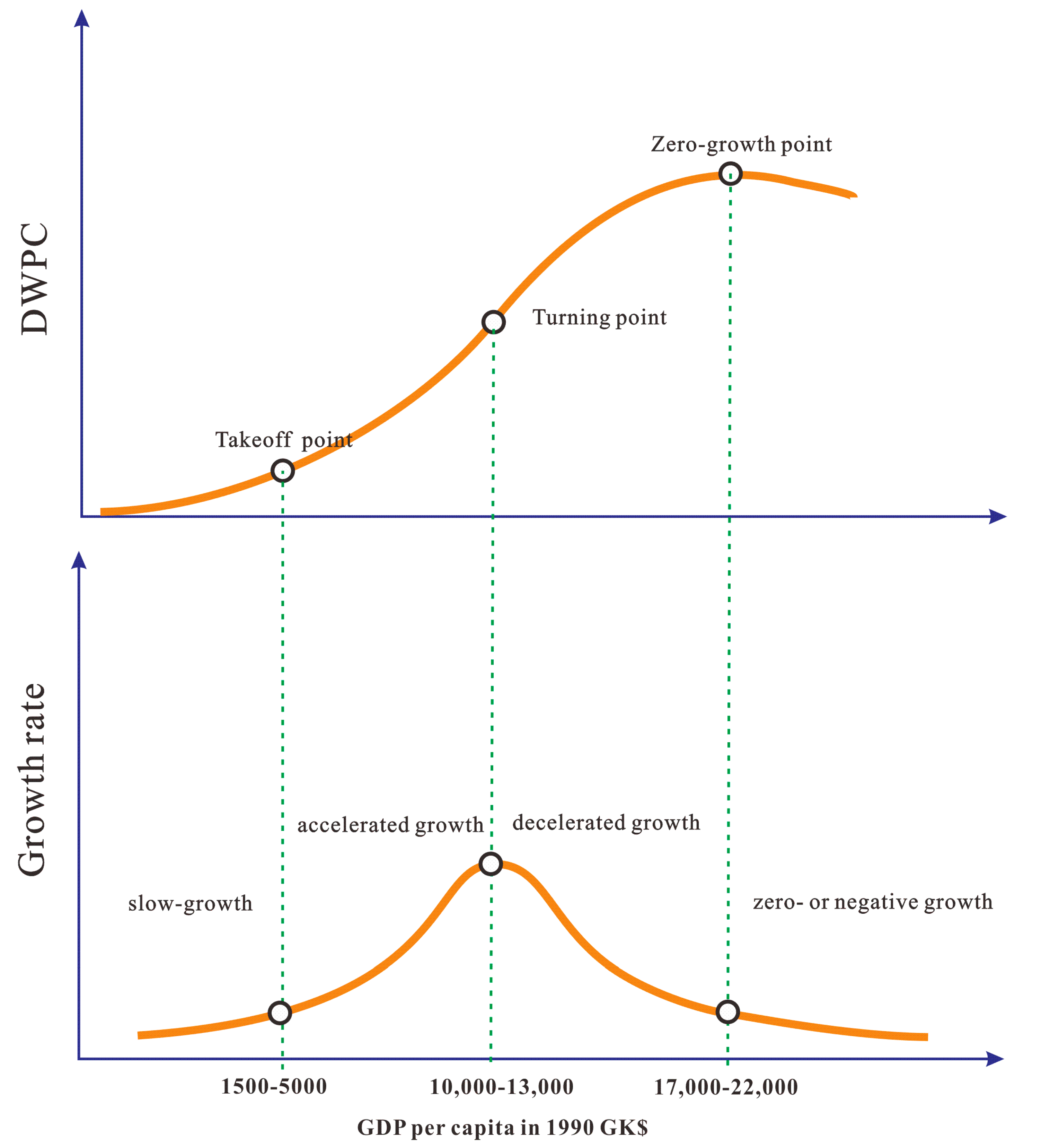
2.2. Mathematical Modeling of the Expanded S-Curve

The expanded S-curve model illustrating the relationship between DWPC and GDP per capita offers a tool to identify critical transitions from one stable state to another during economic development. A mathematical technique is employed to describe the expanded S-curve model. According to the expanded S-curve in previous studies [20,21,29], the relationship between DWPC (W) and GDP per capita (G) can be expressed as follows:

$$W-W_i=A\frac{\exp \left[{\alpha }_1\left(G-G_i\right)\right]-\exp \left(-{\alpha }_3\left(G-G_i\right)\right)]}{2\cos \mathrm{h}\left[{\alpha }_2\left(G-G_i\right)\right]}$$

(1)

where α₁, α₂, and α₃ are the exponential constraints, and A is the amplitude of the equation. W_i and G_i are the corresponding turning points on the expanded S-curve for DWPC and GDP per capita, respectively. Equation (1) is expressed as a hyperbolic tangent function.

Then, the linearity changes before the takeoff point, around the turning point, and after the zero-growth point are derived from Equation (1) as Equations (2)–(4).

$$W-W_i=A+A\left({\alpha }_2-{\alpha }_3\right)\left(G-G_i\right)=A+{\rho }_l\left(G-G_i\right)$$

(2)

$$W-W_i=0.5A\left({\alpha }_1+{\alpha }_3\right)\left(G-G_i\right)={\rho }_i\left(G-G_i\right)$$

(3)

$$W-W_i=A+A\left({\alpha }_1-{\alpha }_2\right)\left(G-G_i\right)=A+{\rho }_v\left(G-G_i\right)$$

(4)

where ρ_l, ρ_i, and ρ_v are the slopes of the curve before the takeoff point, around the turning point, and after the zero-growth point, respectively. They can be calculated from the systems of Equations (5)–(7):

$${\alpha }_1=\frac{{\rho }_l+2{\rho }_i+{\rho }_v}{2A}$$

(5)

$${\alpha }_2=\frac{{\rho }_l+2{\rho }_i-{\rho }_v}{2A}$$

(6)

$${\alpha }_3=\frac{-{\rho }_{l+}2{\rho }_i-{\rho }_v}{2A}$$

(7)

Equation (1) has a first-order partial derived from 0 at the zero-point of the S-curve:

$$\tanh \left[{\alpha }_1\left(G_v-G_i\right)\right]\tan \mathrm{h}\left[{\alpha }_2\left(G_V-G_i\right)\right]={\alpha }_1{\alpha }_2^{-1},\frac{dW}{dG}=0$$

(8)

By substituting Equations (5) and (6) into Equation (8), Equation (9) can be obtained

$$\tanh \left({\phi }_1{A}^{-1}\right)\tanh \left({\phi }_2{A}^{-1}\right)={\phi }_3$$

(9)

where

$${\phi }_1=0.5\left({\rho }_l+{\rho }_i+{\rho }_v\right)\left(G_v-G_i\right)$$

(10)

$${\phi }_2=0.5\left({\rho }_l+2{\rho }_i-{\rho }_v\right)\left(G_v-G_i\right)$$

(11)

$${\phi }_3=\frac{{\rho }_l+{\rho }_i+{\rho }_v}{{\rho }_l+2{\rho }_i-{\rho }_v}$$

(12)

In summary, the W_i, G_i, ρ_l, ρ_i, and ρ_v were from research data, and the A, α₁, α₂, and α₃ were from the equations.

3. Results

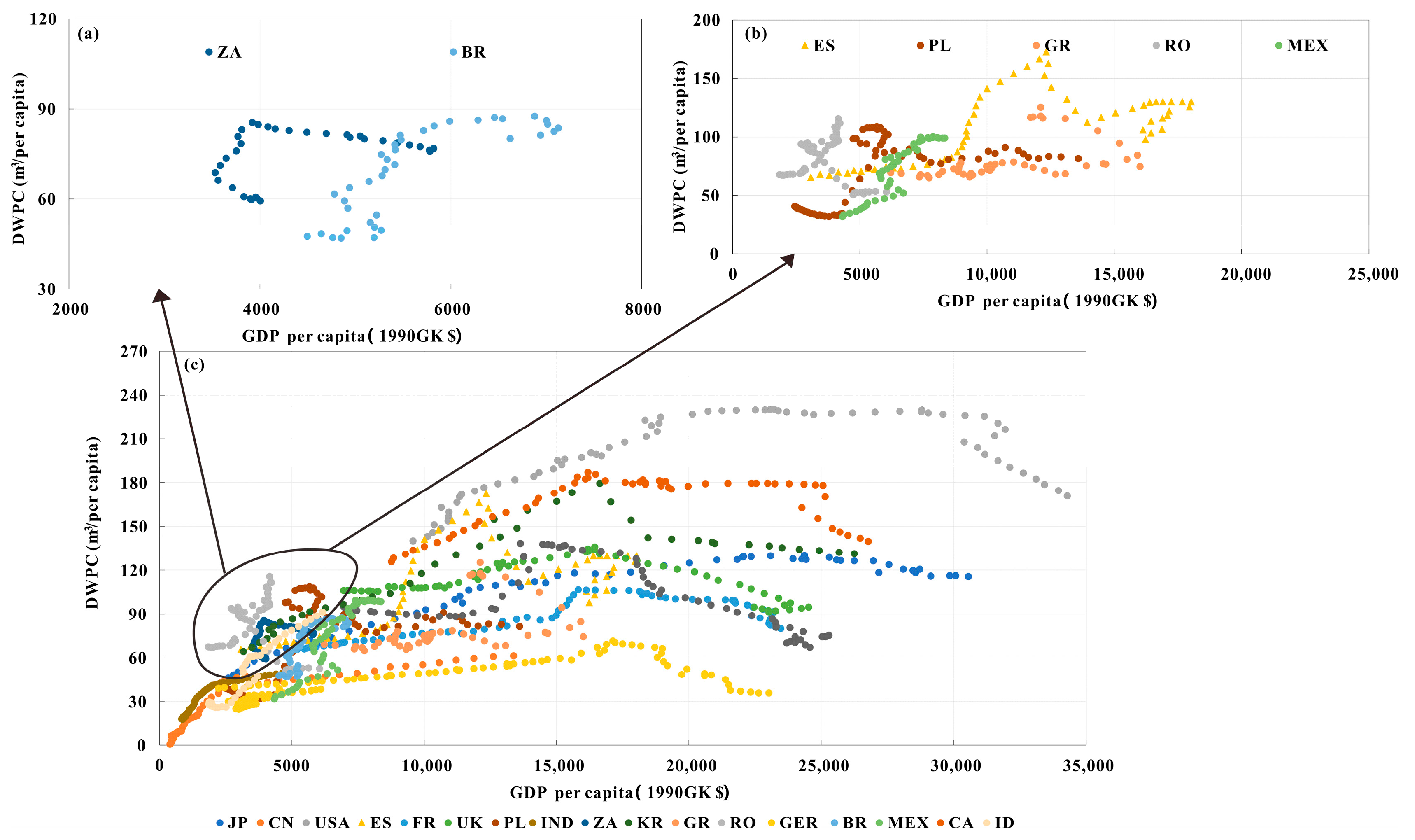
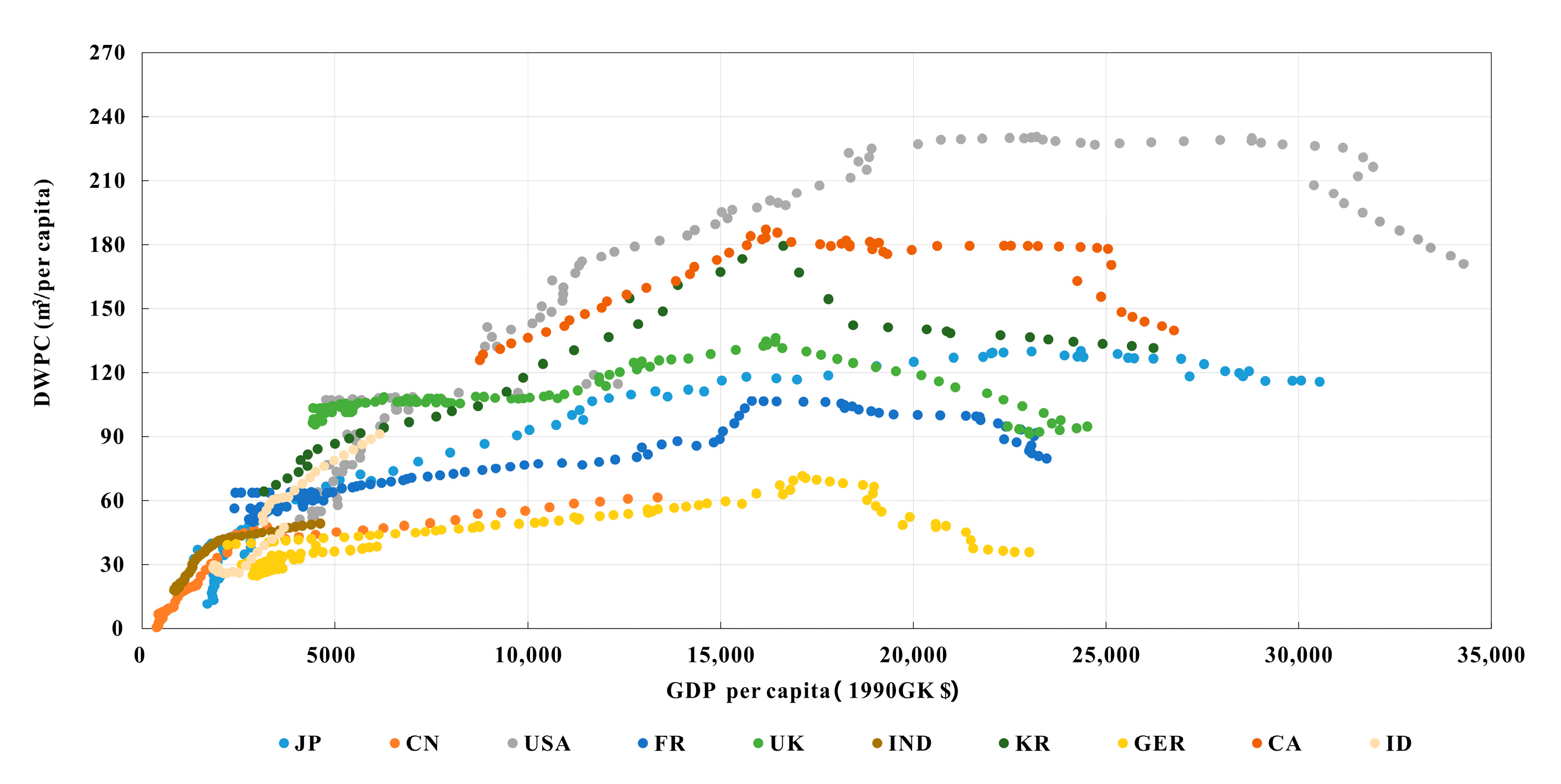
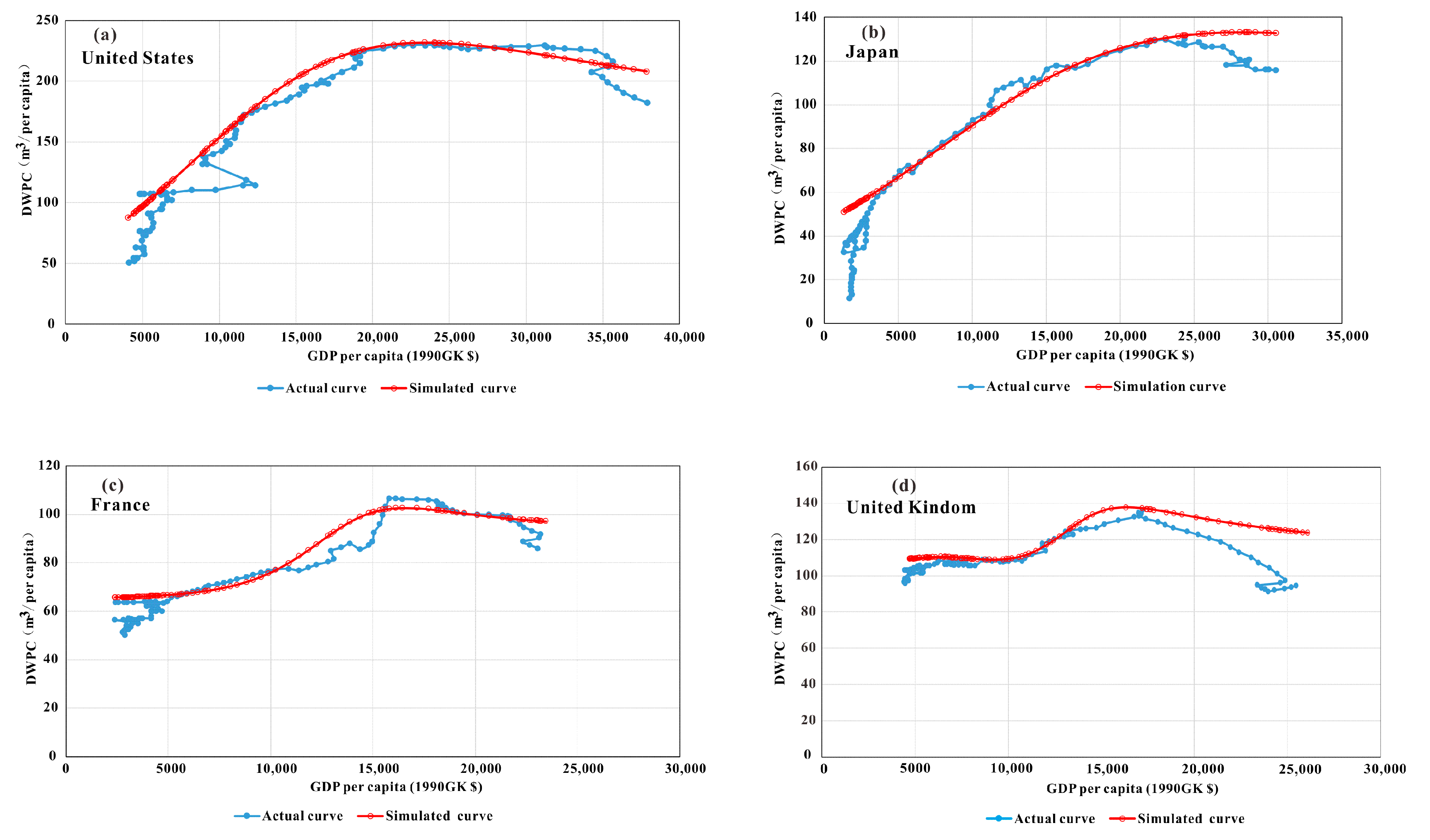
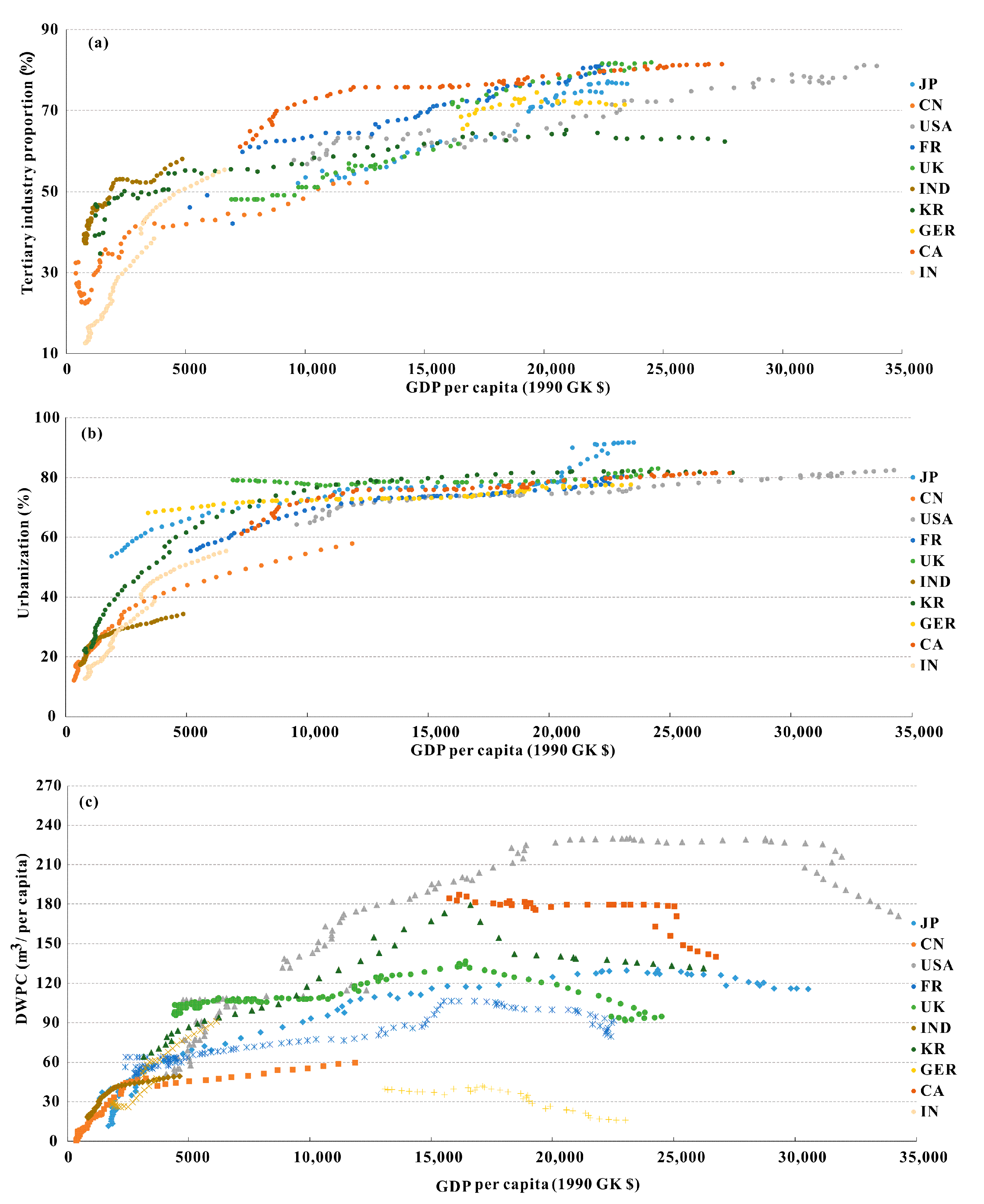
3.1. Expanded S-Curve in Typical Developed Countries

According to the universal equation, the expanded S-curve equations of the DWPC were established for four typical countries as Equations (13)–(16), which were the US, Japan, UK, and France, respectively.

(1)

US

$$W=170+181\times \frac{\exp \left[0.000311\times \left(G-11,500\right)\right]-\exp \left[-0.0000872\left(G-11,500\right)\right]}{2\cosh \left[0.000088\left(G-11,500\right)\right]}$$

(13)

(2)

Japan

$$W=95+90\times \frac{\exp \left[0.0000338\times \left(G-11,000\right)\right]-\exp \left[-0.0000668\left(G-11,000\right)\right]}{2\cosh \left[0.0000673\left(G-11,000\right)\right]}$$

(14)

(3)

UK

$$W=120+30\times \frac{\exp \left[0.000395\times \left(G-13,000\right)\right]-\exp \left[-0.000311\left(G-13,000\right)\right]}{2\cosh \left[0.000395\left(G-13,000\right)\right]}$$

(15)

(4)

France

$$W=90+35\times \frac{\exp \left[0.00000763\times \left(G-12,000\right)\right]-\exp \left[-0.000825\left(G-12,000\right)\right]}{2\cosh \left[0.000178\left(G-12,000\right)\right]}$$

(16)

Figure 4 gives the expanded S-curve simulation for these four typical countries.

The changing trajectories of DWPC with GDP per capita in these countries generally experienced three stages.

For the US in Figure 4a, the first stage was before the GDP per capita of USD 6500 in 1930 during Great Depression, and its economy sequence entered a special period with a winding curve until World War II. The DWPC maintained a flat trend during the first stage. In the second stage, the DWPC in the US kept growing to a high level of 230 m³ in 1990, with a GDP per capita of USD 20,000. After the GDP per capita of USD 35,000 in 2000, the DWPC started to decrease due to technology improvement, with the wide use of dishwashers and water-saving toilets. The efficiency improvements dramatically reduced the water usage.

Japan, in Figure 4b, showed a similar evolution pattern. The DWPC decreased distinctly during World War II in 1940s with a GDP per capita of around USD 2500, and it dropped to 32 m³ with an annual decreasing rate of 7%. Then, with the post-war construction in 1950 with GDP per capita around USD 3500, the economic development model enabled Japan to enter a rapid development process of urbanization. From 1990 to 2000, after 40 years of linear growth, the DWPC in Japan peaked at approximately 120 m³ with a GDP per capita of USD 20,000. After 2000, more efficient appliances and fixtures contributed to significant reductions in DWPC in Japan, with the same reduction trends in US.

France’s and Britain’s economic development was similar to that of US and Japan in the first stage, as shown in Figure 4c, d. They were stagnant for a long time after World War I and World War II before the 1950s. Meanwhile, the DWPC showed stationary trends until 1950. Then the DWPC in these two countries developed differently. For France, the DWPC showed no variation around 65 m³ until 1970, with a GDP per capita of USD 11,000. Then it started to experience a slight increase due to the soaring urbanization rate. In the third stage, the DWPC in France diminished from 106 m³ after 2000 with a GDP per capita of USD 20,000 due to the application of water-saving machines on a large scale. The DWPC variations in UK were directly related to the evolution of water bureau management, which was further propelled by urbanization development. In the late 1960s with a GDP per capita above USD 10,000, the DWPC increased from 113 m³ with the increasing urbanization rate and population, and the management framework of water in the UK was optimized to improve the water efficiency. So, from 1970 to 1990, with a GDP per capita of between USD 11,000 and USD 18,000, an increase in the DWPC of between 115 m³ to 138 m³ was evident in the UK. In 1980s, with the stagflation in economics, the UK government published the Government White Paper on Privatization of Water Industry in 1986 and the top 10 water industries in the UK completed the privatization in 1989, which led to an increase in water prices and a decrease in DWPC in the 1990s with a GDP per capita of above USD 18,000 [30].

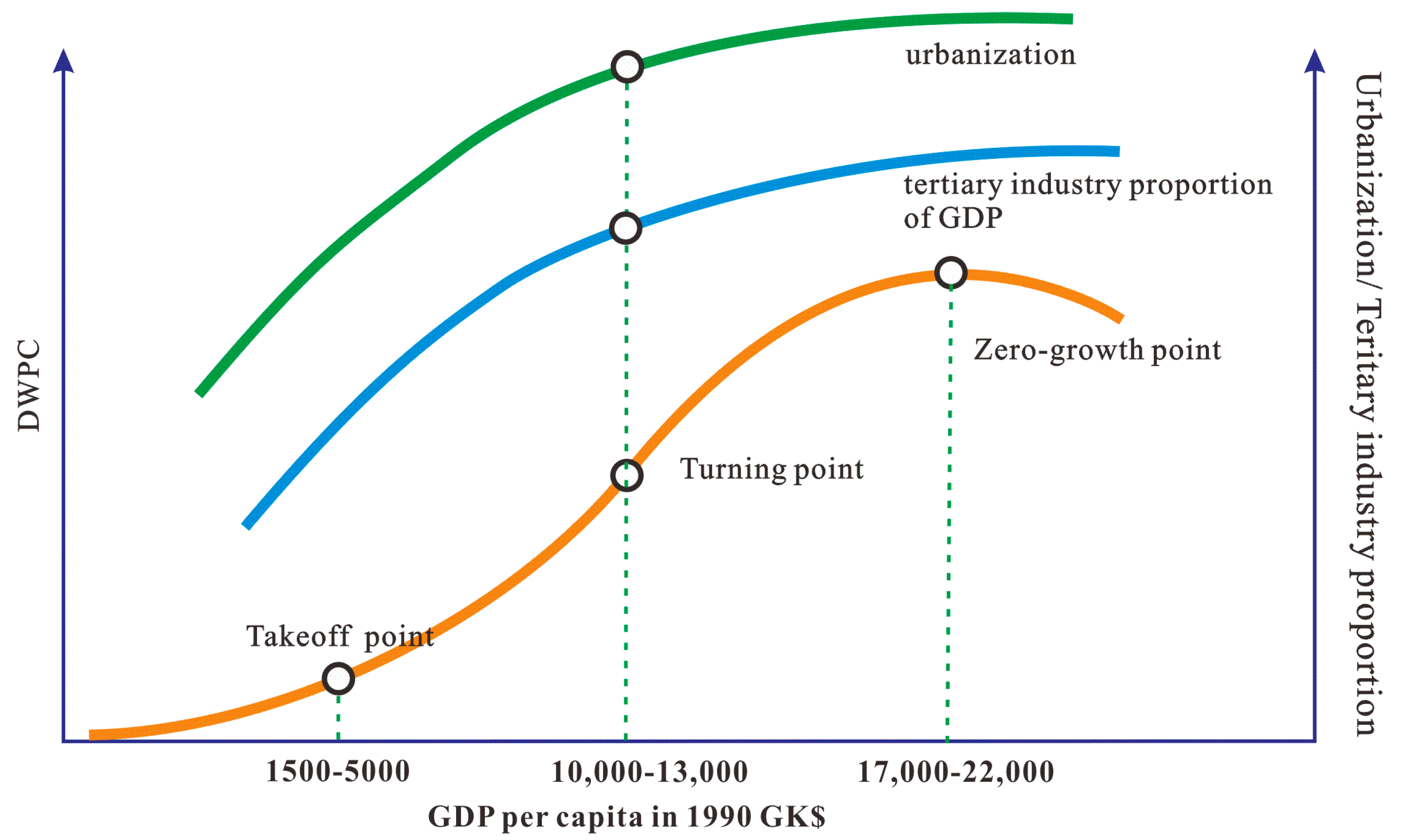
3.2. Implication of the Expanded S-Curve Model

According to the correlation analysis of the increase in DWPC and GDP per capita in Section 2.2 and Section 3.1, we can conclude that the expanded S-curve can be calibrated with three key points, which are the takeoff point, the turning point, and the zero-growth point. Meanwhile, the long-term DWPC trends with GDP per capital were also divided into four stages according to the growth rate transition, including slow growth, accelerated growth, decelerated growth, and zero/negative growth. Figure 5 shows the key points and stages of the S-curve, and the points for each country are summarized in

Table 2. Key points of expanded S-curve for each country (1990 GK in USD).

Country	Takeoff Points GDP per Capita	Turning Points GDP per Capita	Zero-Growth Points GDP per Capita
US	4000–4200	10,100–11,500	20,000–22,000
UK	4500–4800	12,000–13,000	17,000–18,000
France	3500–3800	12,000–13,000	19,000–20,500
Japan	3000–3500	10,000–11,000	22,000–23,000
China	2000–2500	11,000–12,000	–
Germany	3200–3800	11,000–12,000	18,000–19,000
India	1500–1800	–	–
Indonesia	2300–2500	–	–
Canada	–	–	19,000–21,000
South Korea	3000–4000	10,000–12,000	18,000–20,000

.

The takeoff point is the starting point for the accelerated growth in DWPC in the range of USD $1500–5000, implying an adjustment of agriculture society to industrial society with the economic boom. Before this takeoff point, the DWPC was in the slow-growth section. The takeoff points for developed economics, such as the UK, the USA, France, and South Korea, occurred after USD 3000, whereas for developing economies, such as India and China, it occurred between USD 1500 and USD 2500. The turning point made an adjustment period of an industrial structure in the process of industrialization, with a GDP of USD 10,000–USD 13,000 for the researched countries without diversity. After the turning point, the growth rate in the DWPC transited from accelerated growth to decelerated growth until the zero-growth point. The zero-growth points were concentrated around USD 17,000–USD 22,000, which indicates that the DWPC entered a zero-growth or slow-decline stage. This is also consistent with the post-industrial stage [20], when the living standards were improved substantially to promote the technical progress of water-saving facilities.

4. Causes for the Changes in Domestic Water Usage

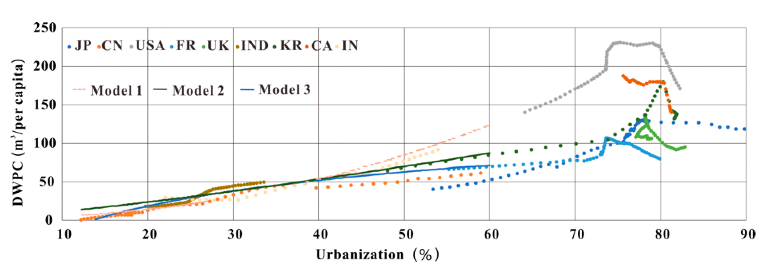
The expanded S-curve model describes the effect of economics on domestic water usage; however, domestic water-usage changes also have a close connection with industrial structure, urbanization, and scientific–technical progress, which were also promoted by economics. The relationship between tertiary industry proportion, urbanization, DWPC, and GDP per capita for these 10 typical countries is summarized in Figure 6. The tertiary industry proportion in Figure 6a and urbanization in Figure 6b both present a similar regularity with GDP per capita, with accelerate growth before a GDP per capita of USD 10,000, decelerated growth between a GDP per capita of USD 10,000 and USD 13,000, and peak value around a GDP per capita of USD 20,000, which is consistent with the DWPC in Figure 6c.

In order to clearly characterize the relationship between these factors, a schematic diagram was established in Figure 7. The three key points of the expanded S-curve were annotated, and the corresponding turning points of tertiary industry proportion and urbanization were also calibrated to compare the corresponding relations.

4.1. Urbanization

The urbanization rate represents the population structure, which has a significant effect on the DWPC. According to previous study, water users in a more urban population in the first trended toward a more water-intensive lifestyle with increasing urbanization rate [13,31,32]. Chen et al. tested the urbanization factor in promoting the DWPC by LMDI [33,34]. The urbanization rate and DWPC showed a positive relationship with conformal key points, as seen in Figure 1 and Figure 7. The urbanization rate can be divided into three stages: It rapidly grew from an urbanization of 20% to 70% before GDP per capita reaches USD 10,000, and then the growth rate decelerated until urbanization reached 80% and the GDP per capita reaches USD 20,000. After this stage, the urbanization was generally saturated, with a stable trend. The turning point for DWPC also occurred between USD 10,000 and USD 13,000, as seen in Figure 7, which is consistent with urbanization. Therefore, we can arrive at the conclusion that urbanization could accelerate domestic water usage.

4.2. Industrial Structure

Domestic water is used in the tertiary industry for urban households, rural households, and commercial service [5,14,24]. As the tertiary industry proportion increases, the urban infrastructure and commercial service would be enhanced with economic development, resulting in an increasing trend in the DWPC. During the industrialization and post-industrialized era, the tertiary industry proportion showed a linear increasing shape. This rapid increasing trend discontinued until a GDP per capita of USD 10,000. Then, it entered a slowly increasing stage between a GDP per capita of USD 10,000 and USD 15,000. The peak of the tertiary industry proportion was around USD 20,000, coinciding with the zero-growth point of the expanded S-curve of DWPC in Figure 6 and Figure 7.

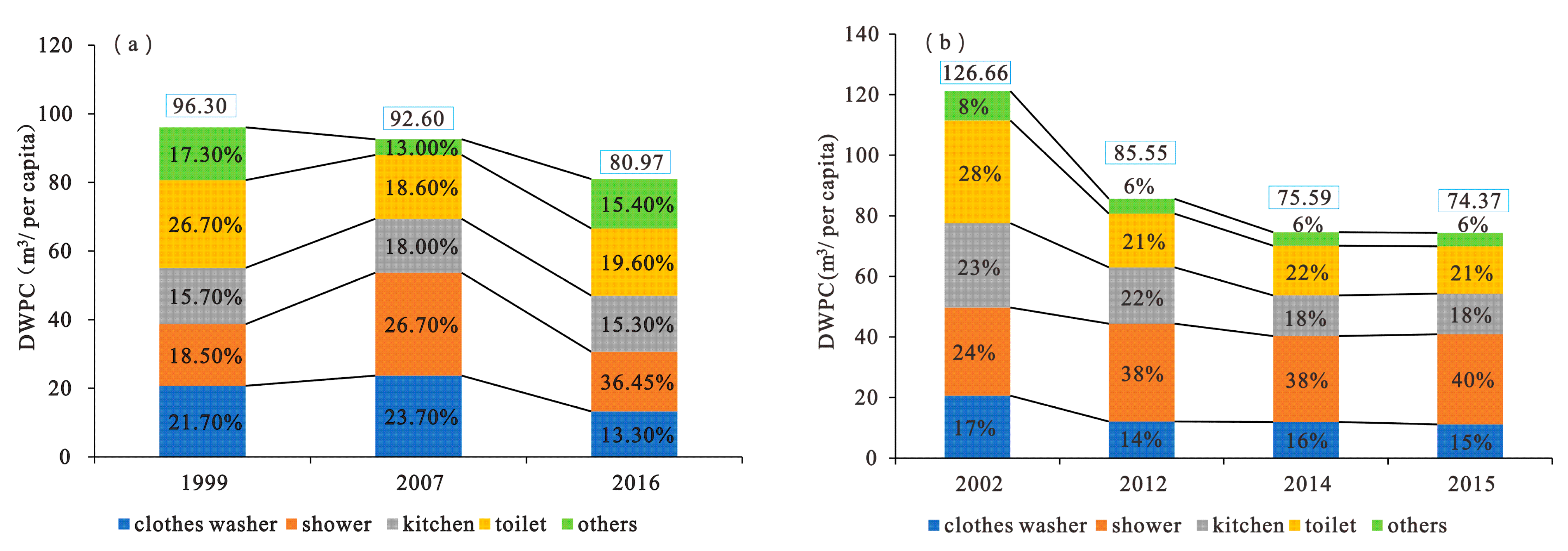
4.3. Technical Progress

The technical progress was usually promoted by the economic development, and it can be considered a main driver for water-usage change [35]. Figure 8 shows the indoor DWPC subsectors for the US and Japan. The indoor DWPC can be divided into five parts, and showers accounted for the greatest share for the US in Figure 8a and toilets account for the greatest share for Japan in Figure 8b. Besides, the shares for kitchen (mainly for dishwashers), clothes washers, and others were also substantial. Between 1990 and 2016, there was a statistically significant reduction in DWPC for toilets in both the US and Japan. According to previous studies, the declines are easy to understand due to the wide use of water-saving toilets. In addition, the increasing the efficiency of fixtures and appliances significantly reduced the amounts of clothes washers and kitchen use. Therefore, the reduction of DWPC after 2000 for most causes could be partly attributed to technological progress.

5. Conclusions

In this paper, we focused on the evaluation of long-term domestic water-usage trends with economic development from typical countries. The relationship between domestic water usage and socio-economic developments on a country scale for the time period from 1900 to 2020 in 10 typical countries was demonstrated. The simulation results show that with the growth in GDP per capita, domestic water per capita showed an expanded S-curve of ‘slow growth–rapid growth–zero growth, or even negative growth, with three key points, which were the takeoff point, turning point, and zero-growth point, respectively. The takeoff point of the expanded S-curve was located at a GDP per capita of USD 1500–USD 5000, according to the different development levels. The turning point was located at a GDP per capita of USD 10,000–USD 13,000, and the zero-growth point was concentrated around a GDP per capita of USD 17,000–USD 22,000, consistent with the post-industrial stage. Besides, the urbanization was proven to accelerate domestic water usage, and the higher tertiary industry proportion of GDP enhanced the domestic water-usage trends. The decreased water usage was attributed to technological progress, with widely used water-saving appliances.

The results of this research show that the expanded S-curve is applicable to the relationship between domestic water usage and economic development on a country scale. We hope this conclusion can contribute to the development of future solutions and strategies for domestic water prediction in different economies or similar economies under different development stages. However, there is still a lot of uncharted territory of the application of the expanded S-curve models. In this paper, only four of 10 typical countries were simulated in detail, and studies on a series of countries with few water usage data are still deficient. We will apply this expanded S-curve model to other countries in our future research, and hope that this model will encourage the efficient and sustainable management of water resources.

References

1. Wada, Y.; de Graaf, I.E.M.; van Beek, L.P.H. High-resolution modeling of human and climate impacts on global water resources. J. Adv. Model. Earth Syst. 2016, 8, 735–763. [Google Scholar] [CrossRef] [Green Version]
2. Haddeland, I.; Heinke, J.; Biemans, H.; Eisner, S.; Flörke, M.; Hanasaki, N.; Konzmann, M.; Ludwig, F.; Masaki, Y.; Schewe, J.; et al. Global water resources affected by human interventions and climate change. Proc. Natl. Acad. Sci. USA 2014, 111, 3251–3256. [Google Scholar] [CrossRef] [PubMed] [Green Version]
3. Owen, A.; Scott, K.; Barrett, J. Identifying critical supply chains and final products: An input-output approach to exploring the energy-water-food nexus. Appl. Energy 2018, 210, 632–642. [Google Scholar] [CrossRef]
4. Xiao, Z.; Yao, M.; Tang, X.; Sun, L. Identifying critical supply chains: An input-output analysis for Food-Energy Water Nexus in China. Ecol. Model. 2019, 392, 31–37. [Google Scholar] [CrossRef]
5. FAO (Food and Agriculture Organization of the United Nations). AQUASTAT. 2020. Available online: https://www.fao.org/statistics/zh (accessed on 20 December 2021).
6. The OECD Environmental Outlook to 2050: The Consequences of Inaction. Available online: https://www.oecd.org/g20/topics/energy-environment-green-growth/oecdenvironmentaloutlookto2050theconsequencesofinaction.htm (accessed on 25 February 2022).
7. Zhou, F.; Bo, Y.; Ciais, P.; Dumas, P.; Tang, Q.; Wang, X.; Liu, J.; Zheng, C.; Polcher, J.; Yin, Z.; et al. Deceleration of China’s human water use and its key drivers. Proc. Natl. Acad. Sci. USA 2020, 117, 7702–7711. [Google Scholar] [CrossRef] [PubMed]
8. Gam, I.; Rejeb, B.J. Micro-economic analysis of domestic water demand: Application of the pseudo-panel approach. Environ. Chall. 2021, 4, 110118. [Google Scholar] [CrossRef]
9. Manouseli, D.; Anderson, B.; Nagarajan, M. Domestic Water Demand During Droughts in Temperate Climates: Synthesising Evidence for an Integrated Framework. Water Resour. Manag. 2018, 32, 433–447. [Google Scholar] [CrossRef] [Green Version]
10. Wang, X.J.; Zhang, J.Y.; Shahid, S.; Xie, W.; Du, C.Y. Modeling domestic water demand in Huaihe River Basin of China under climate change and population dynamics. Environ. Dev. Sustain. 2018, 20, 911–924. [Google Scholar] [CrossRef]
11. Meng, X.M.; Tu, L.P.; Yan, C.; Wu, L.F. Forecast of annual water consumption in 31 regions of China considering GDP and population. Sustain. Pro. Consum. 2021, 21, 713–736. [Google Scholar]
12. Marta, S.V. Modeling residential water demand: An approach based on household demand systems. J. Environ. Manag. 2020, 261, 109921. [Google Scholar]
13. David, B.L.; Bogaart, P.W.; Kram, T.; Vries, B. Long-term water demand for electricity, industry and households. Environ. Sci. Policy 2016, 55, 75–86. [Google Scholar]
14. World Bank Group. 2022. Available online: https://data.worldbank.org.cn/indicator/NY.GDP.MKTP.KD (accessed on 24 February 2022).
15. Guo, W.Y.; Liu, T.; Dai, F.; Xu, P. An improved whale optimization algorithm for forecasting water resources demand. Appl. Soft Comput. 2020, 86, 105925. [Google Scholar] [CrossRef]
16. Zhang, W.S.; Zhou, L.F.; Cheng, Q. Eco-environmental Demand for Water in Wetlands at Liaohe Estuary. J. Irrig. Drain. 2017, 36, 122–130. [Google Scholar]
17. Integrated Assessment of Global Environmental Change with IMAGE 3.0: Model Description and Policy Applications. Available online: https://www.pbl.nl/en/publications/integrated-assessment-of-global-environmental-change-with-IMAGE-3.0PBL (accessed on 11 December 2021).
18. Rathnayaka, K.; Malano, H.; Arora, M.; Georgeb, B.; Maheepalac, S. Prediction of urban residential end-use water demands by integrating known and unknown water demand drivers at multiple scales. Resour. Conserv. Recycl. 2017, 118, 1–12. [Google Scholar] [CrossRef]
19. Verhulst, P.F. Notice sur la loi que la population suit dansson accroissement: Correspondence. Math. Phys. 1983, 10, 113–121. [Google Scholar]
20. Wang, A.J.; Wang, G.S.; Zhou, F.Y. The Limits and Cycles of the Growth of Energy and Mineral Resources Consumption. Acta Geosic. Sin. 2017, 38, 1–10. [Google Scholar]
21. Gao, X.R.; Wang, A.J.; Liu, G.W.; Liu, C.H.; Yan, K. Expanded S-Curve Model of a Relationship Between Crude Steel Consumption and Economic Development: Empiricism from Case Studies of Developed Economies. Nat. Resour. Res. 2019, 28, 547–562. [Google Scholar] [CrossRef]
22. Zuo, Q.T. Interval S-model for forecasting per capita domestic water consumption. J. Hydrau. Eng. 2008, 39, 351–354. [Google Scholar]
23. Florke, M.; Kynast, E.; Barlund, I.; Eisner, S.; Wimmer, F. Domestic and industrial water uses of the past 60 years as a mirror of socio-economic development: A global simulation study. Global Environ. Change 2013, 23, 144–156. [Google Scholar] [CrossRef]
24. USGS (United States Geological Survey). 2021. Available online: https://www.usgs.gov/mission-areas/water-resources/science/water-use-united-states?qt-science–center–objects=0#qt-science–center–objects (accessed on 22 February 2022).
25. European Statics. 2022. Available online: https://ec.europa.eu/eurostat (accessed on 21 February 2022).
26. German Association of Energy and Water Industries. Available online: https://www.eureau.org/about/members/germany-bdew (accessed on 18 December 2021).
27. Gleick, P.H.; Palaniappan, M. Peak water limits to freshwater withdrawals and use. Proc. Natl. Acad. Sci. USA 2010, 107, 11155–11162. [Google Scholar] [CrossRef] [Green Version]
28. Shiklomanov, I.A.; Rodda, J.C. World Water Resources at the Beginning of the 21st Century; International Hydrology Series; Cambridge University Press: Cambridge, UK, 2003. [Google Scholar]
29. Wang, A.; Wang, G.; Chen, Q.; Yu, W.; Yan, K.; Yang, H. S-curve model of relationship between energy consumption and economic development. Nat. Resour. Res. 2015, 24, 53–64. [Google Scholar] [CrossRef]
30. The Development of the Water Industry in England and Wales; Ofwat: Birmingham, UK, 2006.
31. He, W.; Wang, Y.L. Calculation of urban water resources utilization efficiency in the Yellow River basin and analysis of its influencing factors. Acta Sci. Circ. 2021, 41, 4760–4770. [Google Scholar]
32. Vieira, P.; Jorge, C.; Cova, D. Assessment of household water use efficiency using performance. Resour. Conserv. Recycl. 2017, 116, 94–106. [Google Scholar] [CrossRef]
33. Chen, L.; Qiao, C.H.; Xia, L.L.; Cai, Y.P.; Yang, Z.F. Changes of domestic water consumption and its driving mechanism in the period of new urbanization in Guangdong. South-North Water Transf. Water Sci. Technol. 2021, 19, 273–280. [Google Scholar]
34. Zhang, Z.; Liu, J.; Cai, B.; Shan, Y.; Zheng, H.; Li, X.; Li, X.; Guan, D. City-level water withdrawal in China: Accounting methodology and applications. J. Ind. Ecol. 2020, 24, 951–964. [Google Scholar] [CrossRef] [Green Version]
35. Residential End Uses of Water, Version 2. Available online: https://www.waterrf.org/resource/residential-end-uses-water-version-2 (accessed on 22 February 2022).
Figure 1. Relationship between GDP per capita and DWPC for (a) South Africa and Brazil; (b) Spain, Poland, Greece, Romania, and Mexico; and (c) all 17 countries.
Applsci 12 06090 g001
Figure 2. Relationship between urbanization and DWPC.
Applsci 12 06090 g002
Figure 3. Relationship between GDP per capita and DWPC for 10 typical countries.
Applsci 12 06090 g003
Figure 4. Expanded S-curve simulation of DWPC and GDP for (a) the United States (b) Japan, (c) France, and (d) the United Kingdom.
Applsci 12 06090 g004
Figure 5. Three key points and four stages with different growth rates of the expanded S-curve.
Applsci 12 06090 g005
Figure 6. Relationships between GDP per capita and (a) tertiary proportion, (b) urbanization, and (c) tertiary proportion of GDP.
Applsci 12 06090 g006
Figure 7. Relationship between key points of expanded S-curve and important indicators of economic and social development.
Applsci 12 06090 g007
Figure 8. DWPC subsector proportions in (a) the US and (b) Japan.
Applsci 12 06090 g008