
Optimization Method for Low Tilt Sensitivity of Secondary Mirror Based on the Nodal Aberration Theory


1
Changchun Institute of Optics, Fine Mechanics and Physics, Chinese Academy of Sciences, Changchun 130033, China
2
Key Laboratory of Airborne Optical Imaging and Measurement, Chinese Academy of Sciences, Changchun 130033, China
3
University of the Chinese Academy of Sciences, Beijing 100049, China
4
Key Laboratory of Space-Based Integrated Information System, Institute of Software, Chinese Academy of Sciences, Beijing 100190, China
*
Author to whom correspondence should be addressed.
Appl. Sci. 2022, 12(13), 6514; https://0-doi-org.brum.beds.ac.uk/10.3390/app12136514
Submission received: 21 May 2022
/
Revised: 20 June 2022
/
Accepted: 22 June 2022
/
Published: 27 June 2022
(This article belongs to the Collection Optical Design and Engineering)
Abstract
:The optical system that combines imaging and image motion compensation is conducive to the miniaturization of aerial mapping cameras, but the movement of optical element for image motion compensation will cause a decrease in image quality. To solve this problem, reducing the sensitivity of moving optical element is one of the effective ways to ensure the imaging quality of aerial mapping cameras. Therefore, this paper proposes an optimization method for the low tilt sensitivity of the secondary mirror based on the Nodal aberration theory. In this method, the analytical expressions of the tilt sensitivity of the secondary mirror in different tilt directions are given in the form of zernike polynomial coefficients, and the influence of the field of view on the sensitivity is expressed in the mathematical model. The desensitization optimization function and desensitization optimization method are proposed. The catadioptric optical system with a focal length of 350 mm is used for desensitization optimization. The results show that the desensitization function proposed in this paper is linearly related to the decrease of sensitivity within a certain range, and the standard deviation of the system after desensitization is 0.020, which is 59% of the system without desensitization. Compared with the traditional method, the method in this paper widens the range of angle reduction sensitivity and has a better desensitization effect. The research results show that the optimization method for low tilt sensitivity of the secondary mirror based on the Nodal aberration theory proposed in this paper reduces the tilt sensitivity of the secondary mirror, revealing that the reduction of the sensitivity depends on the reduction of the aberration coefficient related to the misalignment in the field of view, which is critical for the development of an optical system for aerial mapping cameras that combines imaging and image motion compensation.
1. Introduction
Aerial mapping cameras play an irreplaceable role in many fields such as environmental protection, ecological resource investigation, land and resources management, geological disaster monitoring, climate impact, and GIS construction by acquiring geographic remote sensing information [1]. When the camera is exposed, there is relative movement between the image of the subject and the photosensitive medium due to vibration, aircraft movement, and camera swings, resulting in image blur and tailing effects, that is, image motion. The optical system that combines imaging and image motion compensating functions is beneficial to simplify the complexity of the optical imaging system and reduce the development cost. In this regard, some applied research has been carried out at home and abroad. Yongsen Xu used the two-mirror system and the lens as two independent parts in the research of the catadioptric optical system based on the fast secondary mirror. The decentering of the secondary mirror was used to realize the image motion compensation of the system, but the influence of the lens was ignored [2]. The image motion compensation is performed by controlling the movement of the secondary mirror of the refractive optical system in the aerial mapping camera visionmap-A3, the ground-based large-aperture FASTTRAC astronomical telescope, and the SIRTF infrared astronomical telescope [3,4,5], but the analysis of optical systems is barely mentioned. Image motion compensation in adaptive optics mainly relies on the detection of the wavefront by the sensor, and the control voltage for the wavefront corrector is calculated by the wavefront controller, and the wavefront corrector is driven to correct the aberration [6]. When the image motion compensation of the optical system does not depend on the precise control of the sensor, the movement of the optical element will degrade the imaging quality, so it is necessary to design an optical system that realizes image motion compensation through the movement of optical element.
Many experts have conducted a series of studies on decreasing tolerance sensitivity. The two processes of optical system optimization and tolerance allocation are separated in the traditional optical design process. The optical design optimization process does not account for the degradation of imaging quality caused by processing (decenter, tilt, surface irregularity, etc.) and assembly (decenter, tilt of components) errors, which leads to the need to redesign the optics when the tolerance requirements are not met. It takes time. As a result, many optical systems are being optimized at the same time as the requirement to reduce the tolerance sensitivity of the optical system, which provides a reference for the design of optical system that realizes image motion compensation through the movement of the optical element. At present, there are two main types of methods to reduce tolerance sensitivity. The first type is to find a system with low sensitivity from the optimization of the initial structure which can be considered as a positive thinking method. The second type is to find a system with low sensitivity from analyzing the variation of the system when the tolerance is introduced. It can be considered as a reverse thinking method. The first type of method mainly includes the global optimization method [7], the multiple structure method [8] and the use of aspherical or free-form surfaces. The second type of method mainly includes the small aberration complementary method [9,10,11], the desensitization method based on the optical path difference and the desensitization method based on the Nodal aberration theory (NAT).
The desensitization method of positive thinking usually focuses on the adjustment of the initial structure. For example, Jose Sasian pointed out, a desensitization lens usually requires more degrees of freedom and change of the lens form [12]. Therefore, the desensitization method of positive thinking usually requires multiple iterations or sensitivity analysis on a sufficient number of samples.
In the desensitization method of reverse thinking, the small aberration complementary method points out that the change of the primary aberration caused by the tolerance is a function of the primary aberration coefficient and the incident angle and the refraction angle. Therefore, Yuanjian Zhang [13] employed the operands of various primary aberrations to optimize the initial structure in the zemax software. Kun Zhang [14] optimized the curvature of each optical surface and balanced the incident angle of each optical surface to achieve small aberration complementation. Yang Zhao et al. [15] proposed a suitable adjustment of the incident angle on the sensitive surface. However, the above designs consider a single angle, and the desensitization effect is limited.
Qingyu Meng [16,17] proposed using optical path difference induced by the tolerance as an evaluation criterion for tolerance sensitivity of optical system. This method derives the optical path difference from the changes of the intersection of the light and the surfaces and the image plane. When there are many components, more optical path changes need to be considered. Therefore, the desensitization method based on the optical path difference is suitable for optical systems with a simple optical structure and few optical components, and the optimization effect of the complex optical system such as aerial mapping camera is poor.
In the desensitization research based on the NAT, Bauman and Schneider [18] established a linear relationship between tolerance, compensator, and wave aberration. Zhiyuan Gu [19] derived the estimated wavefront aberration for a given surface eccentricity and tilt tolerance based on NAT and established an optical system performance evaluation model. The above methods are all based on improving the performance evaluation of the optical system, which has strong versatility and a small calculation amount. However, it has some drawbacks. The analytical derivation of the methods mentioned above is insufficient. In order to realize the matrix operation, Bauman and Schneider ignore the quadratic term of the aberration field decenter vector, and Zhiyuan Gu’s optimization does not analyze the dependence of the sensitivity of the optical component on the field of view.
Based on the NAT of the misaligned system, the analytical expression of the tilt sensitivity of the secondary mirror in different tilt directions is given in the form of zernike polynomial coefficients. This paper takes the aberration coefficient related to the misalignment as the key factor to characterize the relationship between the sensitivity of the optical system and the field of view, proposes a desensitization function with the aberration coefficient and the field of view as the core, and establishes a design method of catadioptric optical system with low tilt sensitivity of secondary mirror. The paper mainly includes the following aspects: Section 2 introduces the image motion compensation model of secondary mirror tilt motion, the NAT of the misaligned system. Section 3 defines the tilt sensitivity, introduces the desensitization function and the desensitization design method. Section 4 takes the catadioptric optical system with a focal length of 350 mm, a field of view angle of ±3° and a secondary mirror’s maximum tilt angle of ±0.1° as an example, and analyzes the changes of the desensitization function, the incident angle, and the relationship between the sensitivity of the aberration term and the field of view during the desensitization process, which verifies the effectiveness of the method in this paper. Section 5 summarizes the whole paper. The analytical expressions of the aberration coefficients related to misalignment when one surface of the optical system is tilted are given in the Appendix A.
2. Theoretical Basis
This section first introduces the image motion compensation model of the secondary mirror tilt motion in the catadioptric optical system, that is, it reveals that the essence of the image motion compensation is that the light from different fields of view is imaged at the same position on the image plane by adjusting the pose of the secondary mirror. Then, NAT of the misaligned system is introduced, that is, the problems existing in the current image motion compensation model are revealed.
2.1. Image Motion Compensation Model of Secondary Mirror Tilt Motion
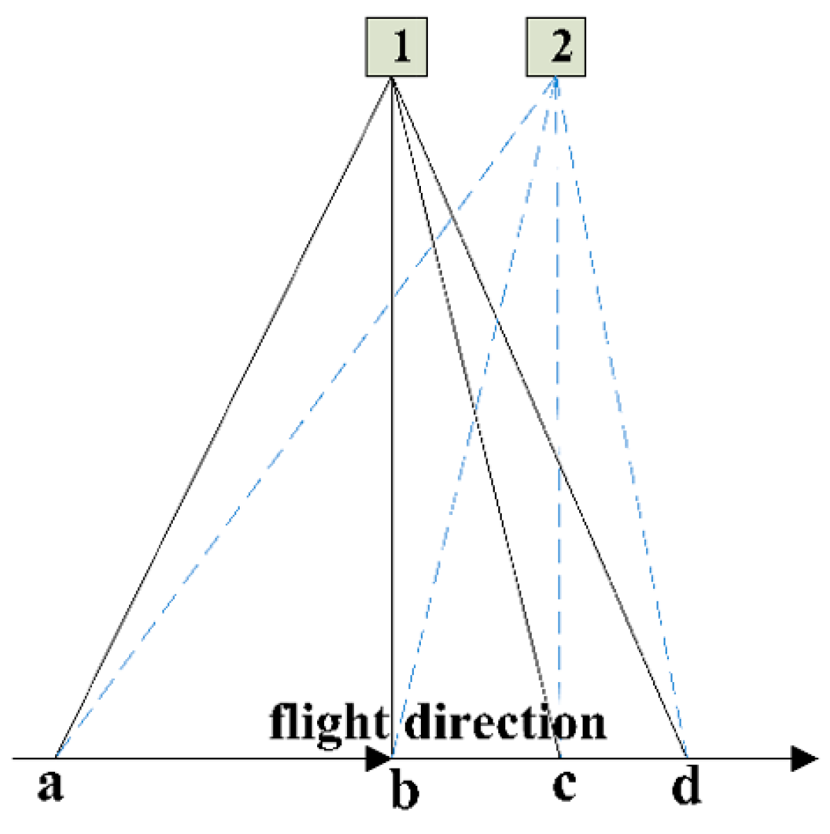
The changes of camera position and field of view during exposure time are shown in Figure 1, where a, b, c and d are the object points on the ground. The camera moves from position 1 to position 2 during the exposure time. The solid black line is the light path from the object point to the camera before exposure, and the blue dotted line is the light path from the object point to the camera after exposure.For the same object point, there is a deviation of the field of view from the optical system before and after exposure. For example, point b is the on-axis field of view for the optical system before exposure, and the off-axis field of view for the optical system after exposure, so the position of the image point relative to the detector is shifted after exposure. In order to ensure that the positions of the same object point imaging relative to the detector before and after the camera movement are the same, it is necessary to ensure that the exit angles of the light rays passing through the optical system of the same object point before and after exposure are the same.
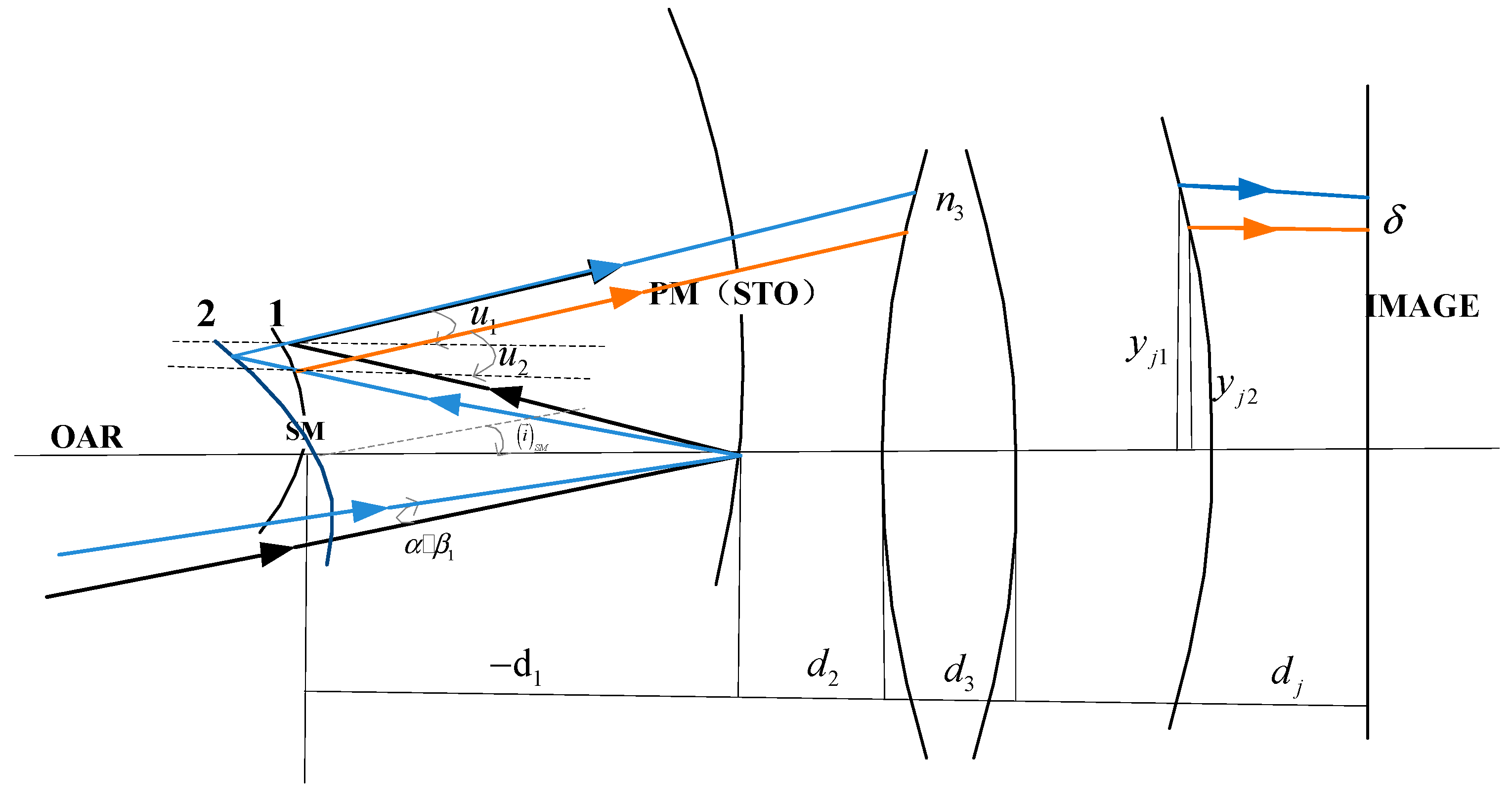
An image motion compensation model of secondary mirror tilt motion is shown in Figure 2. The black light in Figure 2 is the light incident to the optical system from the object point before exposure, and the blue light is the light incident to the optical system from the same object point after exposure. PM is the primary mirror, SM is the secondary mirror, is the angle between the exit ray and the optical axis ray (OAR), d is the surface distance, y is the height of the light on the surface, and i is the inclination angle of the secondary mirror. If the change of the field of view angle of the same object point before and after exposure is , and the angular magnification of the front correction lens is , then the angle of the light on the primary mirror changes as . When the image motion compensation is not performed, the secondary mirror is at pose 1, the exit angles of the black light and the blue light through the optical system are different, that is, , and the distance of the exit lights (blue ray and orange ray) on the image plane is the amount of image shift . The secondary mirror is tilted so that the lights emitted from the same object point through the optical system before and after exposure are the same, that is, the blue light in the Figure 2, and the image motion compensation is realized. Therefore, the amount of image shift caused by the movement of the camera from position 1 to position 2 during the exposure time can be compensated by the tilt movement of the secondary mirror from pose 1 to pose 2.
Based on the above analysis, it can be concluded that the current principle of image movement compensation is that the light from different fields of view is imaged at the same position on the image plane by adjusting the pose of the secondary mirror. In order to ensure the image quality of the camera, it is necessary to reduce the difference of the image quality of different fields of view. However, in the process of image motion compensation, the pose adjustment of the secondary mirror will change the aberration distribution in the effective field of view. Therefore, analyzing the aberration field distribution during the pose adjustment process is essential for optimizing the catadioptric optics with low sensitivity of the secondary mirror.
2.2. The NAT of Misaligned System
When the secondary mirror of the catadioptric optical system is tilted, the optical system can be regarded as a misaligned optical system. Based on NAT, the total aberration of misaligned system is equal to the sum of the aberration contribution of each surface in the system, but the center of the aberration field is offset, and the offset is represented by the aberration field decenter vector [20]. Based on the third-order NAT, the system wave aberration equation when the secondary mirror is tilted can be expressed as follows [21]:
where represents the corresponding wave aberration coefficient, which are respectively (spherical aberration), (coma), (astigmatism), (field curvature) and (distortion). represents the normalized field vector on the image plane, represents the normalized pupil vector on the exit pupil, represents the aberration field decenter vector (related to the tilt angle of the secondary mirror).
Referring to (1), it can be seen that the spherical aberration has nothing to do with the field of view vector, so the spherical aberration is not affected by the tilt and eccentricity of the component. The spherical aberration characteristics of the system remain unchanged before and after the misalignment. The small eccentricity or tilt of the optical element has little effect on the curvature of field, and the distortion does not affect the sharpness of the image. Therefore, coma and astigmatism are the focus of this paper to reduce the tilt sensitivity of the secondary mirror.
3. Desensitization Optimization Function and Desensitization Design Method
This section proposes a solution to the problems existing in the image motion compensation model in Section 2: first, the tilt sensitivity is defined, and then the description model of the desensitization optimization function is established and the desensitization design method is proposed.
3.1. Definition of Tilt Sensitivity
Based on the NAT of the misaligned system, the change of coma and astigmatism before and after the secondary mirror is tilted is defined as tilt sensitivity. In the research on reducing tolerance sensitivity, Zhiyuan Gu expanded the terms of third-order coma and astigmatism to obtain the inherent aberrations of the system and the aberrations introduced by the tilt or eccentricity of the components [19], but the dependence of the sensitivity of the optical component on the field of view is not clear. Therefore, this paper uses vector multiplication to expand the third-order coma and astigmatism. The zernike polynomial coefficients are decomposed into the product of the field of view matrix and the misalignment matrix by matching the expanded third-order coma and astigmatism with the zernike polynomial. Third-order coma and astigmatism coefficients of the zernike polynomial are expressed in the same matrix, as follows [22]:
Among them, and are the x and y components of the aberration field decenter vector, respectively. represents the astigmatism coefficient when the optical system is coaxial, and represent the astigmatism coefficients introduced by the first-order term of misalignment, and represent the astigmatism coefficients introduced by the square term of misalignment, represents the coma coefficient when the optical system is coaxial. and represent the coma coefficients introduced by the first-order term of misalignment. The derivation method of the aberration coefficient related to the misalignment has been relatively mature, and the specific steps are shown in the Appendix A.
Therefore, the tilt sensitivity is the changes of coma and astigmatism coefficients of the zernike polynomial before and after tilt, namely , , , . i represents the different tilt directions of the secondary mirror, respectively +x, −x, +y and −y, j represents different fields of view. , , and represent the coma and astigmatism coefficients of the zernike polynomial before tilt (secondary mirror on-axis). , , and represent the coma and astigmatism coefficients of the zernike polynomial after tilt. Since the tilt angle of the secondary mirror is usually very small, the third-order aberration is the main aberration of the misaligned system, ignoring the effect of higher-order aberration. Therefore, the contributions of the third-order coma and astigmatism to the zernike polynomial coefficients should be considered when the secondary mirror is tilted. When the secondary mirror is located on the axis, there is no quantity related to the the aberration field decenter vector, that is, , we can get the coma and astigmatism coefficients of the zernike polynomial before tilt as follows:
The variation of the zernike polynomial coefficients of the third-order coma and astigmatism with the field of view for the different tilt directions of the secondary mirror will be derived below. The difference between the zernike polynomial coefficients when the secondary mirror is tilted and the secondary mirror on the axis is the contribution of the aberration to the sensitivity.
3.1.1. Sensitivity When the Secondary Mirror Is Tilted around the X-Axis
Referring to (3), when the secondary mirror is tilted around the x-axis, , then , we can get the coma and astigmatism coefficients of the zernike polynomial when the secondary mirror is tilted about the x-axis, as follows:
The sensitivity matrix of the secondary mirror tilt around the x-axis can be obtained by subtracting (4) from (5), as follows:
3.1.2. Sensitivity When the Secondary Mirror Is Tilted around the Y-Axis
Referring to (3), when the secondary mirror is tilted around the y-axis, , then , we can get the coma and astigmatism coefficients of the zernike polynomial when the secondary mirror is tilted about the y-axis, as follows:
The sensitivity matrix of the secondary mirror tilt around the y-axis an be obtained by subtracting (4) from (7), as follows:
Referring to (6) and (8), the change of the zernike polynomial coefficients with the field of view when the secondary mirror is tilted can be obtained. The zernike polynomial coefficients are functions of the aberration coefficients related to misalignment and the field of view. and represent the sensitivity of the astigmatism terms, and represent the sensitivity of the coma terms.
Refer to (3), and are related to the product of the third-order coma coefficient and the aberration field decenter vector; , and are related to the third-order astigmatism coefficient and the aberration field decenter vector. Obviously, the effect of reducing the sensitivity of the optical system can be achieved by reducing the third-order aberration coefficient of each surface. The aberration coefficient is related to the incident angle and height of the edge ray and the incident angle of the chief ray, the refractive index of the lens and the “aplanatic” parameter. It is consistent with the previous research to reduce the sensitivity of the optical system by optimizing the incident angle and deflection angle and balancing the primary aberration coefficients of each surface.
The difference is that tilt sensitivity has a different relationship to the field of view. The sensitivity of the astigmatism terms is linearly related to the field of view, where , are the coefficients of the first-order term, and the is constant term. The sensitivity of the coma terms has nothing to do with the field of view, where , are the coefficients of the coma terms. The sensitivity of the aberration term in the field of view is measured by the aberration coefficient related to the misalignment. For systems with the same tilt angle and different tilt directions, the absolute values of , , , and are equal, that is, the first-order coefficients of the sensitivity of the astigmatism terms, the constant term of the sensitivity of the astigmatism terms and the coefficients of the coma terms are equal in absolute values. Considering the different correlation between the sensitivity of the aberration term and the field of view, the tilt sensitivity of the secondary mirror in the optical system has different weights in different fields of view. Therefore, the relationship between the third-order aberration coefficient, the aberration field decenter vector and the field of view must be considered comprehensively to meet the requirement of reducing the tilt sensitivity of the secondary mirror in the catadioptric optical system.
3.2. Desensitization Optimization Function
In order to achieve the desensitization effect, it is necessary to minimize the change of the zernike coefficient before and after the tilt of the secondary mirror. The desensitization optimization is carried out with the root mean square of the sensitivity of the coma and astigmatism terms and the desensitization function is as follows:
i represents the different tilt directions of the secondary mirror, respectively +x, −x, +y and −y, j represents different fields of view. Refer to Section 3.1, when the secondary mirror is tilted around the x-axis or the y-axis, its tilt sensitivity has the same expression, and when the tilt angles are the same and the tilt directions are different, the absolute values of the coefficients are the same, so the above formula can be simplified as:
, and are the aberration coefficients related to the misalignment, so the desensitization function can be expressed as a function of the aberration coefficient related to the misalignment and the field of view. When the field of view is determined, the effect of reducing the sensitivity can be achieved by reducing the value.
3.3. Desensitization Design Method
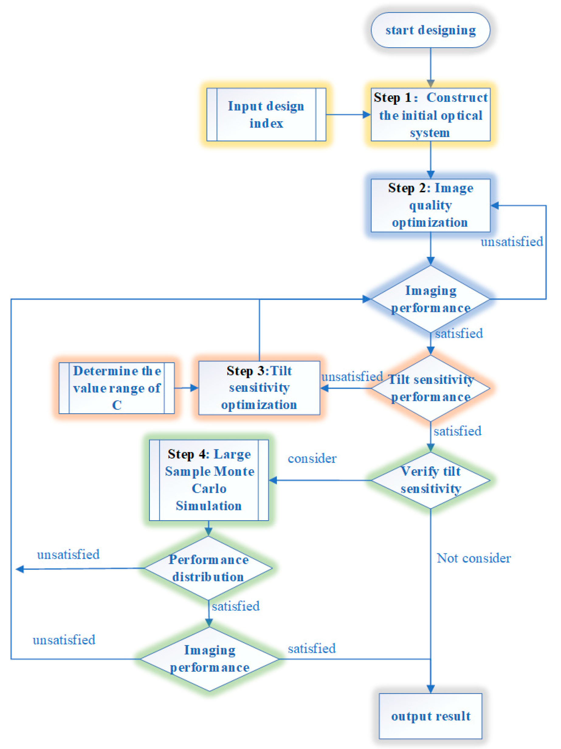
In this section, a design method for a catadioptric optical system with low tilt sensitivity of the secondary mirror is proposed. The design process is shown in Figure 3, which is mainly divided into four steps:
- Construct the initial system according to the design index of the optical system;
- Imaging performance optimization. In the optimization process, parameters such as thickness, radius, conic coefficient are used as optimization variables, and the structure size of the optical system is controlled at the same time. For example, if the designed system is a catoptric system, considering the requirements of processing, it is necessary to limit the interval between the primary and secondary mirrors, and at the same time, the distance from the last surface to the image surface can not be too small. After optimization, the system that meets the imaging performance requirements enters the desensitization design step;
- Tilt sensitivity optimization. The core of the desensitization design process is to control the desensitization function . Within the value range of , continuously reduce the value of until the optical system meets the requirements of imaging quality and low tilt sensitivity of the secondary mirror at the same time, and then output the system;
- Verify tilt sensitivity. To avoid the special case where the optimized system is low sensitivity, a sensitivity simulation of a large sample of the optical system can be performed. The core of this step is to establish a Monte-Carlo simulation of a large sample of the system, and to evaluate the results of the Monte-Carlo analysis. If the imaging quality requirements are met and the performance distribution is concentrated, the design can be output as the final result. If the requirements are not met, the system needs to be optimized again.
4. Simulation Experiment and Analysis of Desensitization Optimization
In this section, taking the catadioptric optical system with a focal length of 350 mm, a field of view angle of ±3° and a secondary mirror’s maximum tilt angle of ±0.1° as an example, the desensitization optimization and analysis are carried out by using the method in this paper and the traditional method to verify the effectiveness of the desensitization design method.
4.1. Desensitization Optimization Based on This Method
This section starts from the design indicators of the optical system, and desensitizes the optical system after the imaging performance optimization.
Since the aerial camera optical system is selected for optimization in this paper, its design indicators must consider various factors. The focal length of an aerial camera is determined by the resolution, flying height and pixel size. The field of view of the optical system is related to the focal length and the size of the detector. The larger the F number of the optical system, the better the signal-to-noise ratio; however, this will increase the weight and volume of the optical system and design will be more difficult. The amount of image shift of an aerial camera is related to many factors such as the speed-to-height ratio, focal length, exposure time, swept angular velocity, and flight attitude of the aircraft. The design index of the aerial camera optical system with image motion compensation of secondary mirror tilt motion is shown in Table 1.
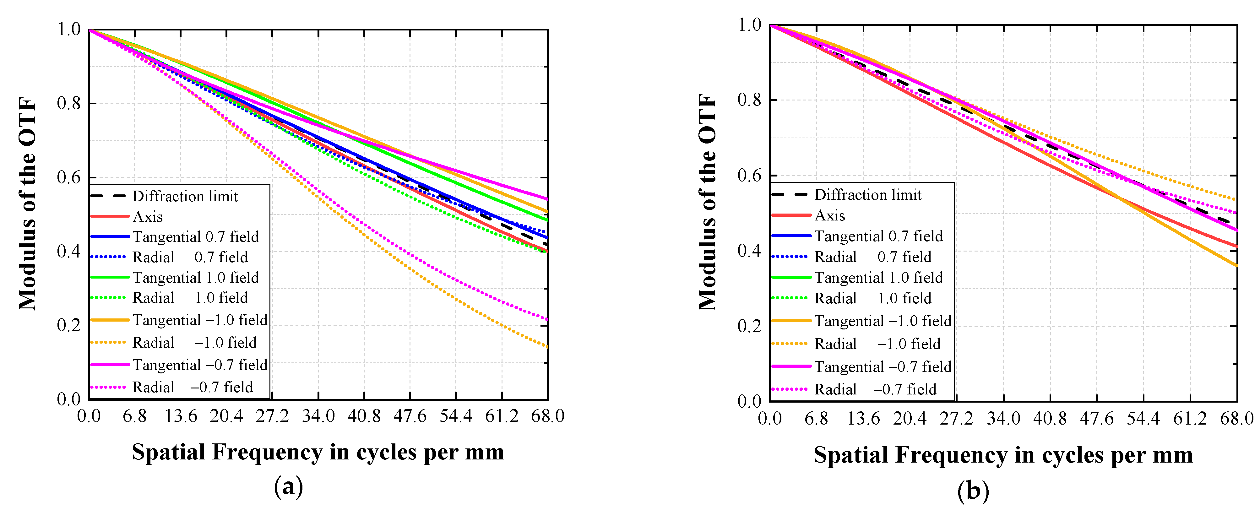
After the imaging performance is optimized, the system is composed of a front correction lens, a primary and a secondary mirror, and a rear correction lens. The H-K9L and TF3 glass materials are combined to eliminate the secondary spectrum. The system realizes the correction of primary aberration and chromatic aberration. Next, the optical system after imaging performance optimization is used as the system without desensitization, and the tilt sensitivity is optimized. The desensitization function is established by macro programming and added to the evaluation function. In the optimization process, it is found that the reduction of the value is beneficial to improve the transfer function of the optical system when the secondary mirror is tilted. Therefore, multiple structures with different tilt directions of the secondary mirror are set up, and the transfer function of the optical system when the secondary mirror is tilted at the maximum angle is greater than 0.3 as the value standard for the minimum value of . The initial value is , when the value is reduced from 127.017 to 49.856, the transfer function of the optical system is greater than 0.3. When the secondary mirror is tilted by 0.1° around the x-axis, the MTF of the optical system without desensitization and after final desensitization are shown in Figure 4.
It can be seen from Figure 4 that, when the secondary mirror is tilted to the maximum angle, the MTF of the optical system after final desensitization is greater than 0.3 at 68 lp/mm, which meets the design requirements.
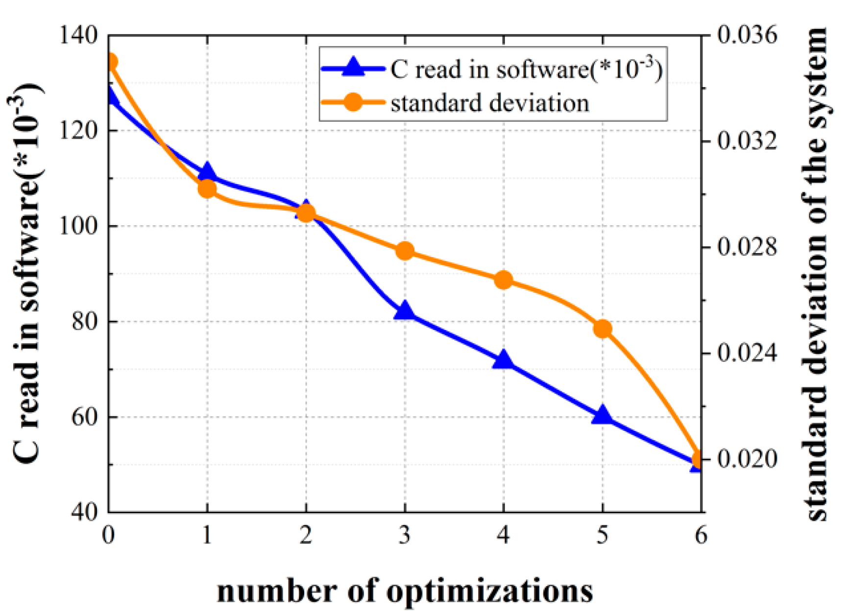
Save the systems in the tilt sensitivity optimization process, and perform a small sample Monte-Carlo analysis (sampling of 200) using only the secondary mirror tilt of 0.1° as the system tolerance. The desensitization optimization process is shown in Figure 5. The abscissa is the optimization times, the left ordinate is the value, and the right ordinate is the standard deviation of the system. The standard deviation is an index to measure the sensitivity of the system. The smaller the standard deviation, the lower the sensitivity.
It can be seen from Figure 5 that when the value is reduced from 127.017 to 49.856, the standard deviation of the system is also decreasing, indicating that the decrease of the value is positively correlated with the decrease of the sensitivity. The standard deviation reduced from 0.35 to 0.020.
4.2. Desensitization Optimization Based on Traditional Methods
The traditional optimization method, also known as the angle-splitting method [23,24], points out that the system sensitivity is replaced by the root mean square of incident and refracted angles of several rays traced to each surface, as follows:
In the formula, and are the incident angle and the refracted angle of the light on the s-plane, respectively, and k is the number of surfaces of the system.
In the optimization process, parameters such as thickness, radius, and conic coefficient are set as optimization variables, and the structural size of the optical system is controlled at the same time. The tilt sensitivity of the secondary mirror is reduced by optimizing the incident angle and refracted angle of the secondary mirror. During the angle reduction process, the performance when the secondary mirror is tilted by 0.1° around the x-axis and standard deviation of the system change as shown in Table 2.
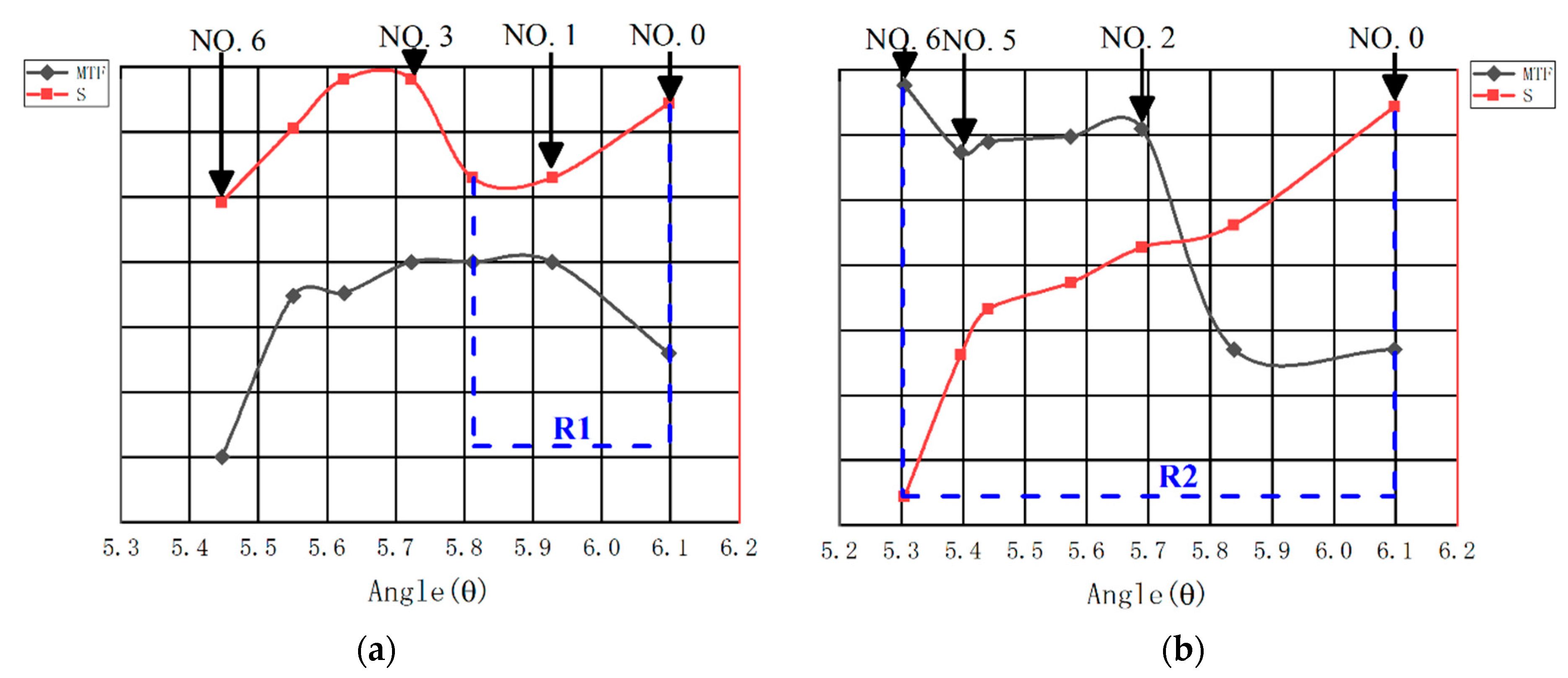
In the process of reducing the angle, the standard deviation of the system and the change of MTF when the secondary mirror is tilted by 0.1° around the x-axis are shown in Figure 6. R1 is the applicable range of angles obtained by the traditional method; R2 is the applicable range of angles obtained by this method.
In general, there is a trade-off relationship between performance and sensitivity, and it is difficult to optimize performance and sensitivity at the same time. The system performance and standard deviation obtained by the traditional method are shown in Figure 6a. In the process of reducing the angle, the reduction of the sensitivity of the solution from NO. 0 to NO. 1 depends on the improvement of the system performance, which reflects the advantage of the corner segmentation method is that the system can achieve the effect of reducing the sensitivity and improving the image quality at the same time. However, the system performance has reached the extreme value in the change of NO. 1 to NO. 3, and the reduction of the angle has no optimization effect on the sensitivity at this time. The performance and sensitivity of NO. 3 to NO. 6 are reduced at the same time, indicating that reducing the angle has no optimization effect on the system performance. By reducing the angle to reduce the sensitivity, it is found that the effective range of its angle is very narrow, only in the range of 0.28°. The system performance and standard deviation obtained by the method in this paper are shown in Figure 6b. The reduction of the sensitivity of the solution from NO. 0 to NO. 2 depends on the improvement of the system performance. The system performance has reached the extreme in the change from the solution NO. 2 to NO. 5, but the sensitivity continues to decrease, indicating that the reduction of the angle is still one of the key factors to reduce the sensitivity at this time. The performance of the solution from NO. 5 to NO. 6 jumps out of the local optimum value, and the sensitivity decreases. Based on the above analysis, it can be obtained that the method in this paper has a wide correlation range between angle and sensitivity, which is 0.793°. The optimal system obtained by the traditional method is NO. 1, and the standard deviation is reduced by 0.003. The optimal system obtained by this method is NO. 6, and the standard deviation is reduced by 0.015. Therefore, the optimization of a single variable angle can only achieve the effect of desensitization and performance improvement in a small range.
4.3. Analysis of Optimization Results
This section analyzes the changes of the system during the desensitization process of the method in this paper from three aspects: the layout of the optical system, the relationship between the sensitivity of the aberration term and the field of view, and the results of the large sample Monte-Carlo analysis.
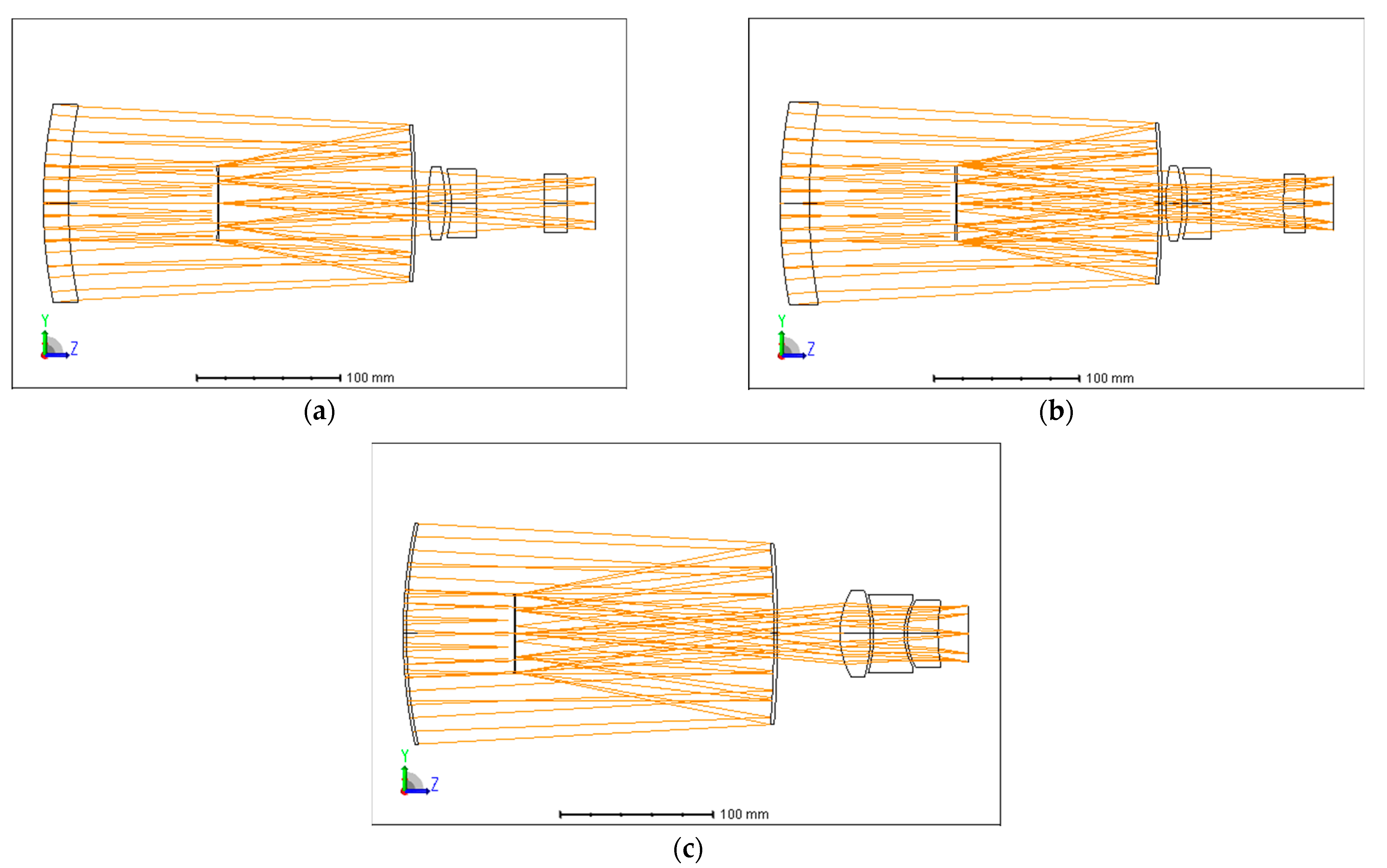
Select the solution of NO. 0 (the system without desensitization), the solution of NO. 1 (the optimized system after one-time desensitization), and the solution of NO. 6 (the optimized system after final desensitization) to analyze the changes in the optical structure during the desensitization process. The layout of the optical system is shown in Figure 7. Figure 7a is the solution of NO. 0, Figure 7b is the solution of NO. 1, and Figure 7c is the solution of NO. 6.
It can be seen from Figure 7 that, for a single lens, the lens form changes after desensitization. The thickness of the first lens is reduced, the third lens is changed from a plano-concave lens to a bi-concave lens, and the curvature of the fourth lens is increased. For the overall change of the system, the rear group lens of the system after final desensitization bears more optical power and has a more compact structure and the change of the lens form is the performance of the system sensitivity reduction.
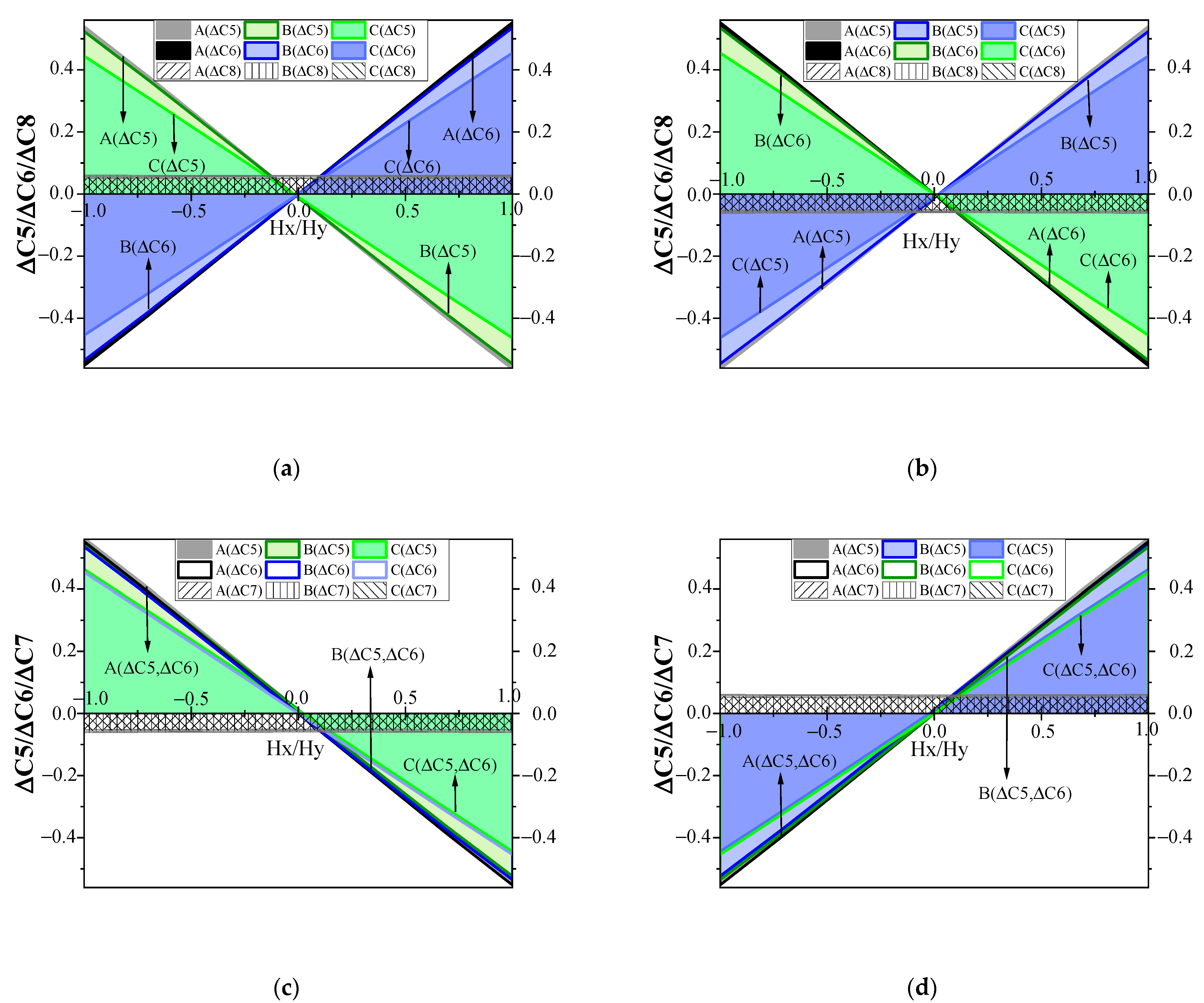
The root of the reduction of the value is the reduction of the sensitivity of the aberration term. The variation of the sensitivity of the aberration term with the field of view is shown in Figure 8. A, B and C represent different systems, corresponding to Figure 7a–c. Figure 8a shows the variation of sensitivity with the field of view when the secondary mirror is tilted by 0.1° around the x-axis, Figure 8b shows the variation of sensitivity with the field of view when the secondary mirror is tilted by −0.1° around the x-axis, Figure 8c shows the variation of sensitivity with the field of view when the secondary mirror is tilted by 0.1° around the y-axis and Figure 8d shows the variation of sensitivity with the field of view when the secondary mirror is tilted by −0.1° around the y-axis. and represent the sensitivity of the astigmatism terms, shown as the edges of the filled color in Figure 8; and represent the sensitivity of the coma terms, shown as the edges of the filled line in Figure 8.
It can be seen from Figure 8 that the sensitivity of the coma term is constant in the full field of view, and the sensitivity of the astigmatism term is linearly related to the field of view. When the secondary mirror is tilted around the x-axis, the slopes of and are opposite to each other, and are equal. When the secondary mirror is tilted around the y-axis, the slopes of and are equal, and are equal. This shows that when the absolute value of the tilt angle (the misalignment) is equal, the first-order coefficients of the sensitivity of the astigmatism terms, and the coefficients of the coma terms are equal in absolute values. and basically intersect in the central field of view, indicating that the constant term of the sensitivity of the astigmatism terms are equal. From the perspective of different systems, and of the A, B, and C systems are approximately equal; and of the B system have a decreasing trend compared with the A system and the linear variation of and with the field of view of the C system being minimal.
It can be seen from Section 2 that the first-order coefficients of the sensitivity of the astigmatism terms are the astigmatism coefficients introduced by the first-order term of misalignment, namely and . The constant term of the sensitivity of the astigmatism terms is the astigmatism coefficients introduced by the square term of misalignment, namely . The sensitivity of the coma terms is the coma coefficients introduced by the first-order term of misalignment, namely and . From the optimization results, it can be seen that the reduction of sensitivity mainly depends on the astigmatism coefficients introduced by the first-order term of misalignment.
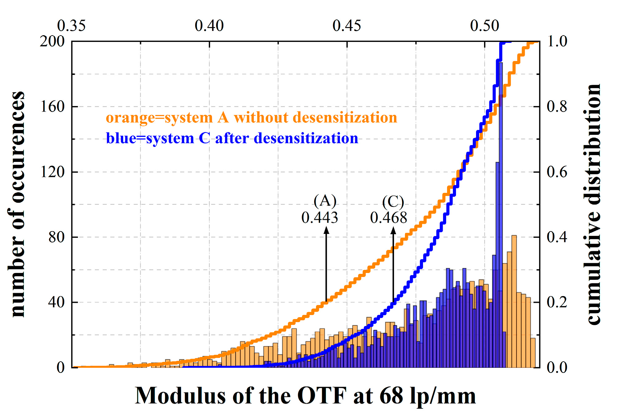
Finally, the performance of system A without desensitization and system C after final desensitization were compared by Monte-Carlo analysis method including 2000 samples, as shown in Figure 9. The abscissa is the MTF, the left ordinate is the number of samples, and the right ordinate is the cumulative distribution.
The histogram of Monte-Carlo results shows that the performance distribution of the system before desensitization is relatively scattered, and the results with the best and worst performances appear in the system before desensitization. For 80% of the MTF, the system without desensitization is above 0.443, and the system after final desensitization is above 0.468. The results obtained before desensitization and after final desensitization are not much different. From the point of view of the cumulative integral curve, when the MTF is high, the slope of the curve of the system after final desensitization is relatively large, that is, the performance distribution of the system is more concentrated under the tilt tolerance. The standard deviation of the system without desensitization is 0.035. The standard deviation of the system after final desensitization is 0.020, which is 59% of the system without desensitization, indicating that the tilt sensitivity of the system after final desensitization is lower. A desensitized system can produce neither very good nor very poor tests. Therefore, for system performance control, desensitized systems are preferable to those optimized only for image quality.
5. Conclusions
In order to ensure the imaging quality of the catadioptric optical system with image motion compensation of secondary mirror tilt motion, this paper establishes an optimization method for the catadioptric optical system with low tilt sensitivity of the secondary mirror based on the NAT of misaligned system. This method expresses tilt sensitivity as the difference of zernike polynomial coefficients before and after the movement which is a function of the aberration coefficient related to the misalignment and the field of view. The sensitivity of the coma terms is constant over the field of view, and the sensitivity of the astigmatism term is linearly related to the field of view. Essentially, the reduction of tilt sensitivity depends on the reduction of the sensitivity of the aberration term across the field of view. In the actual design, the desensitization optimization algorithm is saved in the form of a macro programming file in the optical design software, which is used as a user-defined function to optimize the optical system. It is suitable for systems with many optical components. Different from previous studies, this method considers the angle comprehensively, and the sensitivity reduction is the result of comprehensively considering the third-order aberration coefficient, the aberration field decenter vector and the field of view. The simulation results reveal that the astigmatism coefficients introduced by the first-order term of misalignment is the main factor to reduce the sensitivity. Compared with the method of reducing the sensitivity by angle optimization, the method in this paper has a wider application range of angles, and the sensitivity reduction effect is better. The optimization example of the catadioptric optical system shows that this method is suitable for reducing the tilt sensitivity of moving optical components. When the effect of decenter needs to be considered, it needs to be redefined in the Appendix A.
Author Contributions
Conceptualization, J.L. and Y.D.; methodology, J.L. and Y.D.; software, J.L.; validation, J.L., Y.D. and Y.C.; formal analysis, J.L.; data curation, M.Z.; writing—original draft preparation, J.L.; writing—review and editing, Y.C.; funding acquisition, Y.D.; supervision, Y.D.; project administration, Y.C.; visualization, G.Y.; resources, G.Y. All authors have read and agreed to the published version of the manuscript.
Funding
This research was funded by High-resolution Measurement Camera Project of China (NO. Y92X1SK190).
Institutional Review Board Statement
Not applicable.
Informed Consent Statement
Not applicable.
Data Availability Statement
Not applicable.
Acknowledgments
The authors would like to express appreciation to the editors and reviewers for their valuable comments and suggestions. The authors are grateful for the support by the High-resolution Measurement Camera Project [grant number Y92X1SK190].
Conflicts of Interest
The authors declare no conflict of interest.
Appendix A
For an optical system with n surfaces, when the surface k is tilted, the aberration field decenter vector of before the the surface k is 0, and the surface k and the subsequent j surfaces have the aberration field decenter vector that is not 0.
The aspheric aberration field decenter vector of surface k is 0, so the aberration field decenter vector of surface k is equal to spherical aberration field decenter vector, as follows [19]:
is the tilt vector of surface k, and is the chief ray incident angle of surface k.
The aberration field decenter vectors of j surfaces behind surface k can be obtained through optical axis ray (OAR) tracing. When j surfaces are all spherical, the aberration field decenter vector of surface j is as follows [19]:
and represent the incident angle of the marginal ray and the chief ray on the j-th surface, and represent the incident height of the marginal ray and the chief ray on the k-th surface. represents the change of the refractive index of the k-th surface, and represents the optical invariant.
According to the seidel aberration formula, the spherical third-order aberration coefficients are as follows:
Therefore,
By , ADE represents the tilt around the x-axis, BDE represents the tilt around the y-axis. By substituting into the expression of the aberration field decenter vector and the above expression, the parametric expressions when the optical element is tilted around the x-axis can be obtained. By substituting into the expression of the aberration field decenter vector and the above expression, the parametric expressions when the optical element is tilted around the y-axis can be obtained.
References
- Zeng, Y. Research on the Development of Foreign Aerial Surveying and Mapping Cameras. Jiangxi Surv. Mapp. 2015, 3, 30–32. [Google Scholar]
- Xu, Y.; Ding, Y. The Catadioptric Optical System with Second Mirror Fast Image Motion Compensation. In Proceedings of the 3rd Outstanding Proceedings Annual Conference on High Resolution Earth Observation, Changsha, China, 7 November 2014. [Google Scholar]
- Pechatnikov, M.; Shor, E.; Raizman, Y. Visionmap A3—Super Wide Angle Mapping System Basic Principles and Workflow. In Proceedings of the 21st ISPRS Congress, Beijing, China, 3–11 July 2008. [Google Scholar]
- Close, L.M.; McCarthy, D.W. Infrared imaging using a tip-tilt secondary mirror. SPIE 1993, 1920, 353–363. [Google Scholar]
- Bottema, M. Impact of Chopping on Image Quality In The SIRTF Telescope. SPIE 1984, 509, 35–43. [Google Scholar]
- Wang, J. Research on Disturbance Model Identification and Optimal Control Technology for Adaptive Optics Systems. Ph.D. Thesis, Department of Signal and Information Processing, Institute of Optoelectronic Technology, Chinese Academy of Sciences, Chengdu, China, 2020. [Google Scholar]
- Rogers, J.R. Using global synthesis to find tolerance-insensitive design forms. In Proceedings of the International Optical Design Conference, Vancouver, BC, Canada, 4–8 June 2006; Volume 6342, p. 63420M. [Google Scholar]
- McGuire, J.P. Designing easily manufactured lenses using a global method. In Proceedings of the International Optical Design Conference, Vancouver, BC, Canada, 4–8 June 2006; Volume 6342, p. 63420O. [Google Scholar]
- Liu, X.; Gong, T.; Jin, G.; Zhu, J. Design method for assembly-insensitive freeform reflective optical systems. Opt. Express 2018, 26, 27798–27811. [Google Scholar] [CrossRef] [PubMed]
- Yang, T.; Jin, G.; Zhu, J. Automated design of freeform imaging systems. Light Sci. Appl. 2017, 6, e17081. [Google Scholar] [CrossRef] [PubMed]
- Jeffffs, M. Reduced manufacturing sensitivity in multi-element lens systems. In Proceedings of the International Optical Design Conference, Tucson, AZ, USA, 3–7 June 2002; Volume 4832, pp. 104–113. [Google Scholar]
- Sasian, J. Lens Desensitizing: Theory and Practice. Appl. Opt. 2022, 61, 62–67. [Google Scholar] [CrossRef] [PubMed]
- Zhang, Y.; Tang, Y.; Wang, P. Method of Tolerance Sensitivity Reduction of Optical System Design. Opto-Electron. Eng. 2011, 38, 127–133. [Google Scholar]
- Zhang, K. Research on the Space Target Measuring Optical System with High Precision and Large Field of View. Ph.D. Thesis, Department of Optical Engineering, Changchun Institute of Optics, Fine Mechanics and Physics, Chinese Academy of Sciences, Changchun, China, 2021. [Google Scholar]
- Zhao, Y.; Gong, Y.; Hu, Y. Method of Tolerance Sensitivity Reduction of Zoom Optical System. Opto-Electron. Eng. 2009, 36, 121–125. [Google Scholar]
- Meng, Q.; Wang, H.; Wang, W. Sensitivity theoretical analysis and desensitization design method for reflective optical system based on optical path variation. Opt. Precis. Eng. 2021, 29, 72–83. [Google Scholar] [CrossRef]
- Meng, Q.; Wang, H.; Wang, W. Desensitization design method of unobscured three-mirror anastigmatic optical systems with an adjustment-optimization-evaluation process. Appl. Opt. 2018, 57, 1472–1481. [Google Scholar] [CrossRef] [PubMed]
- Bauman, B.J.; Schneider, M.D. Design of optical systems that maximize as-built performance using tolerance/compensator-informed optimization. Opt. Express 2018, 26, 13819–19840. [Google Scholar] [CrossRef] [PubMed]
- Gu, Z.; Wang, Y.; Yan, C. Optical system optimization method for as-built performance based on nodal aberration theory. Opt. Express 2020, 28, 7928–7942. [Google Scholar] [CrossRef] [PubMed]
- Buchroeder, R.A. Tilted Component Optical Systems. Master’s Thesis, Department of Optical Engineering, University of Arizona, Tucson, AZ, USA, 1976. [Google Scholar]
- Thompson, K. Description of the third-order optical aberrations of near-circular pupil optical systems without symmetry. J. Opt. Soc. Am. A 2005, 22, 1389–1401. [Google Scholar] [CrossRef] [PubMed]
- Li, L. Alignment Technique for Off-Axis Reflective Systems Based on Zernike Vector Polynomials. Ph.D. Thesis, Department of Optical Engineering, Changchun Institute of Optics, Fine Mechanics and Physics, Chinese Academy of Sciences, Changchun, China, 2020. [Google Scholar]
- Isshiki, M.; Gardner, L.; Gregory, G.G. Automated control of manufacturing sensitivity during optimization. In Proceedings of the Optical Systems Design, St. Etienne, France, 30 September 2003; Volume 5249, pp. 343–352. [Google Scholar]
- Isshiki, M.; Sinclair, D.C.; Kaneko, S. Lens design: Global optimization of both performance and tolerance sensitivity. In Proceedings of the International Optical Design Conference, Vancouver, BC, Canada, 4–8 June 2006; Volume 6342, p. 63420N. [Google Scholar]
Figure 1.
The changes of camera position and field of view during exposure time.

Figure 2.
Image motion compensation model of secondary mirror tilt motion.

Figure 3.
Flow diagram of catadioptric optical system with low tilt sensitivity of secondary mirror.
Figure 3.
Flow diagram of catadioptric optical system with low tilt sensitivity of secondary mirror.

Figure 4.
The MTF of the optical system when the secondary mirror is tilted by 0.1° around the x-axis (a) without desensitization, (b) after final desensitization.
Figure 4.
The MTF of the optical system when the secondary mirror is tilted by 0.1° around the x-axis (a) without desensitization, (b) after final desensitization.

Figure 5.
Desensitization optimization process diagram.

Figure 6.
Variation of MTF when the secondary mirror is tilted by 0.1° around the x-axis and standard deviation of system (a) traditional method (b) this method.
Figure 6.
Variation of MTF when the secondary mirror is tilted by 0.1° around the x-axis and standard deviation of system (a) traditional method (b) this method.

Figure 7.
Layout of the optical system of (a) the solution of NO. 0, (b) the solution of NO. 1 and (c) the solution of NO. 6.
Figure 7.
Layout of the optical system of (a) the solution of NO. 0, (b) the solution of NO. 1 and (c) the solution of NO. 6.

Figure 8.
The variation of the sensitivity of the aberration term with the field of view when the secondary mirror is tilted by (a) 0.1° around the x-axis, (b) −0.1° around the xaxis, (c) 0.1° around the y-axis and (d) −0.1° around the y-axis.
Figure 8.
The variation of the sensitivity of the aberration term with the field of view when the secondary mirror is tilted by (a) 0.1° around the x-axis, (b) −0.1° around the xaxis, (c) 0.1° around the y-axis and (d) −0.1° around the y-axis.

Figure 9.
Monte-Carlo tolerance analysis results of the optical system A without desensitization and C after final desensitization.
Figure 9.
Monte-Carlo tolerance analysis results of the optical system A without desensitization and C after final desensitization.


Table 1.
Indexes of the aerial camera.
| Focal length/mm | 350 |
| F number | 4 |
| Full field of view | 6° |
| Spectral range/ Primary wavelength/ | 0.48–0.65 0.58 |
| MTF (68 lp/mm) | ≥0.30 |
| Maximum tilt angle of secondary mirror | ±0.1° |
Table 2.
List of solutions.
| Solution | MTF (The Secondary Mirror Is Tilted by 0.1° Around the X-Axis) | Standard Deviation | |
|---|---|---|---|
| No. 0 | 6.098 | 0.135 | 0.035 |
| No. 1 | 5.928 | 0.208 | 0.032 |
| No. 2 | 5.812 | 0.196 | 0.032 |
| No. 3 | 5.723 | 0.205 | 0.036 |
| No. 4 | 5.625 | 0.176 | 0.036 |
| No. 5 | 5.551 | 0.174 | 0.034 |
| No. 6 | 5.447 | 0.044 | 0.031 |
Publisher’s Note: MDPI stays neutral with regard to jurisdictional claims in published maps and institutional affiliations. |
© 2022 by the authors. Licensee MDPI, Basel, Switzerland. This article is an open access article distributed under the terms and conditions of the Creative Commons Attribution (CC BY) license (https://creativecommons.org/licenses/by/4.0/).
Share and Cite
MDPI and ACS Style
Li, J.; Ding, Y.; Cai, Y.; Yuan, G.; Zhang, M. Optimization Method for Low Tilt Sensitivity of Secondary Mirror Based on the Nodal Aberration Theory. Appl. Sci. 2022, 12, 6514. https://0-doi-org.brum.beds.ac.uk/10.3390/app12136514
AMA Style
Li J, Ding Y, Cai Y, Yuan G, Zhang M. Optimization Method for Low Tilt Sensitivity of Secondary Mirror Based on the Nodal Aberration Theory. Applied Sciences. 2022; 12(13):6514. https://0-doi-org.brum.beds.ac.uk/10.3390/app12136514
Chicago/Turabian StyleLi, Jing, Yalin Ding, Yiming Cai, Guoqin Yuan, and Mingqiang Zhang. 2022. "Optimization Method for Low Tilt Sensitivity of Secondary Mirror Based on the Nodal Aberration Theory" Applied Sciences 12, no. 13: 6514. https://0-doi-org.brum.beds.ac.uk/10.3390/app12136514
Note that from the first issue of 2016, this journal uses article numbers instead of page numbers. See further details here.