Determining the Severity of Open and Closed Cracks Using the Strain Energy Loss and the Hill-Climbing Method

Abstract

Evaluating the integrity of structures is an important issue in engineering applications. The use of vibration-based techniques has become a common approach to assessing cracks, which are the most frequently occurring damage in structures. When involving an inverse method, it is necessary to know the influence of the position and the geometry of the crack on the modal parameter changes. The geometry of the crack, both in size and shape, defines the damage severity (DS). In this study, we present a method (DS-SHC) used for estimating the DS for closed and open transverse cracks in beam-like structures using the intact and damaged beam deflections under its weight and a Stochastic Hill Climbing (SHC) algorithm. After describing the procedure of applying DS-SHC, we calculate for a prismatic cantilever beam the severities for different crack types and depths. The results are tested by comparing the DS obtained with DS-SHC with those acquired from dynamic tests made using professional simulation software. We obtained a good fit between the severities determined in these two ways. Subsequently, we performed laboratory experiments and found that the severities obtained with the DS-SHC method can accurately predict the frequency changes due to the crack. Hence, these severities are a valuable tool for damage detection.

1. Introduction

Numerous damage detection methods have been developed in recent decades. These are usually applied to check sensitive structures or structures involving high risk in operation. Depending on the principle of the non-destructive testing method applied, there are two main categories: local methods and global methods [1]. Local methods require approximate knowledge of the position of the damage and can only be applied to accessible areas. The advantage of these methods is the high accuracy in characterizing the type and size of the defect. However, in most cases the position of the structural damage is unknown before the control is performed. For this reason, global control is essential to observe the occurrence or propagation of damage and thus to characterize the state of integrity of structures, especially complex or large ones. Global damage detection methods use information regarding the vibration of the structure [2,3]. The essence of damage detection based on changes in the dynamic behavior of the structure is the deterministic relationship between physical and modal parameters [4]. More specifically, the presence of defects causes changes in the modal parameters of the structure, and these changes are used to diagnose, locate, and estimate the severity of the damage [5].

The simplest case of structural damage is the transverse crack in an isotropic and homogeneous structure. For this type of damage, non-destructive testing aims to identify its position and estimate its depth. The position of the crack can be unequivocally related to the change of a modal parameter, namely the modal curvature [6]. The case of the crack depth is different, as it cannot be directly related to a modal parameter. However, there is an indirect link between the depth of the crack and the natural frequency of the structure, and both parameters mentioned above are related to the damage severity.

Deterministic damage detection methods fall into two categories: the finite element approach and the continuous approach. In most damage detection cases that use the finite element method, the structure is divided into identical elements that extend over the entire cross-section of the structure. All elements have the mechanical and physical characteristics of the intact structure, except one or a few elements where there is a defect. The defective element, simulating the crack, commonly has a reduced Young’s modulus. In most of the studies, the number of finite elements in the model is taken between 4 and 30, and the reduction of the elastic modulus of an element is in the range of 20% to 50%, see, for example, [7,8,9,10,11]. This approach requires centering the crack on an element and, therefore, the precision of assessing damage is determined by the distribution of the elements along the beam [10]. However, the biggest problem with using this method is the lack of a definite relationship between the severity of the damage and the depth of the crack, because the relationship depends on the size of the elements used for discretization [12]. When examining the methods proposed in the literature, we observed that the dependency between the reduction in the size of the crack and the stiffness is rarely considered. In general, the authors limit the study to finding the element in the beam with the lower Young modulus value [13]. When damage detection is applied to trusses, finding the member with the lower Young modulus is usually the target.

Another approach to modeling damage is to divide the structure into two segments that are linked by a rotational massless spring. This equivalent spring introduces four more unknowns in the system, which are determined from the continuity conditions [14]. The correlation between the crack depth determining the local compliance and the equivalent spring stiffness is found using fracture mechanics results [15]. There are many mathematical relations to express the compliance functions relative to the crack depth available in the literature, see for instance [16,17,18,19]. Involving this approach, damage detection consists of fitting the position and the stiffness for one finite element to obtain by calculus similar natural frequencies to those obtained for the damaged beam by experiments [20]. Analyzing a multitude of compliance functions, we found significant differences between the results achieved for certain crack depths, resulting in a negative influence on the accuracy of the damage assessment methods based on this approach.

Recent research focuses on detecting damage by involving artificial intelligence (AI). Examples of current methods aiming to detect damage in beams can be found in [21,22,23], while in [24,25,26] are exemplified methods applicable to complex structures. These approaches are based on the analysis of the vibration signal parameters in the time domain (acceleration, damping), or in the frequency domain (mode shapes and curvatures, frequencies). The training data are obtained from simulation or measurements, thus initially it involves a limited number of damage cases. If for a given structure it is possible to determine the relationship between the damage parameters and the vibration signal parameters, it is possible to generate a multitude of damage cases [27] including the case of imperfect clamping. In this way, the training process can be improved, and the AI algorithms provide more accurate prediction results.

In prior research, we determined a mathematical relation to finding the severity of closed or open cracks [28]. The data used to calculate the severity are the deflections at the free end of a cantilever beam for the healthy and damaged case, respectively. Because the severity is an intrinsic parameter of the damage, it is the same for beams with any boundary conditions. Thus, it is sufficient to determine the severity just for the cantilever beam. For the reasons presented in the next section, determining the deflection of the damaged beam implies regression analysis followed by extrapolation. Thus, the results are influenced by the nature of the regression curve used and may vary accordingly.

In this paper, we propose a mathematical relation to calculate the effect of a crack located anywhere on the beam on its deflection. This relation is used to find the damage severity from static tests made with cracks having a random position on the beam. Instead of regression analysis, we use Stochastic Hill Climbing (SHC) as an optimization method. To the best of our knowledge, there is no research to determine the severity of the defect using AI. Using this procedure to find the damage severity we avoid obtaining results that depend on the analysis strategy, thus these are very accurate.

The paper is structured as follows: the expression of the cracked beam deflection is deduced in Section 2, then we present the procedure to determine the damage severity (Section 3) and the achieved results for several beams and crack dimensions (Section 4), while in Section 5 we test the capacity of estimating frequency changes due to damage by involving the achieved damage severities. Finally, we present the conclusions of the research in Section 6.

2. The Expression of the Cracked Beam Deflection

This section presents a method for determining the deflection at the free end of a cantilever beam with a crack. The challenge faced when attempting to evaluate damages is that the effect of the crack, both on the deflection as well as on the natural frequencies, is different when it is placed in different positions along the beam. However, the crack has the biggest effect when it is in the beam slice in which the mechanical stresses are highest, i.e., where the bending moment reaches its maximum value. In the case of the cantilever beam, this location is the fixed end. In prior research [29], we have determined a method for assessing the severity of transverse cracks, considering the deflection of a cantilever beam in the intact state and when it is altered by a breathing crack of known depth a that is located at the fixed end. This mathematical relation is:

$$\gamma (a)=\frac{\sqrt{\delta (a,0)}-\sqrt{{\delta }_u}}{\sqrt{\delta (a,0)}}$$

(1)

In Equation (1) we denoted: $\gamma (a)$ the severity of a crack with depth a located at the fixed end; $\delta (a,0)$ the deflection at the free end of the cantilever beam having a crack with depth a at the fixed end (index 0 stays for location x = 0 mm); ${\delta }_u$ the deflection of the intact beam at the free end.

It is easy to determine the deflection at the free end for the beam with a constant cross-section subjected to dead mass, as:

$${\delta }_u=\frac{\rho Ag{L}^4}{8EI}$$

(2)

Here, $\rho$ is the volumetric mass density, A is the cross-sectional area, g is the gravity, E is Young’s modulus and I is the second moment of inertia. This deflection is also easy to be obtained from a finite element analysis (FEA).

Regarding the deflection of a beam affected by cracks, there are no analytical relations for calculating the deflection. Thus, it becomes difficult to determine the severity of cracks. Problems also occur when involving FEA. For a crack positioned at the fixed end, the stresses and deformations of the beam can manifest only on one side of the crack, unlike the case where the crack is located elsewhere along the beam. Thus, the rotation in the cracked region is smaller than that achieved for a crack located in the neighborhood. This has as a consequence a smaller deflection than expected at the free end. 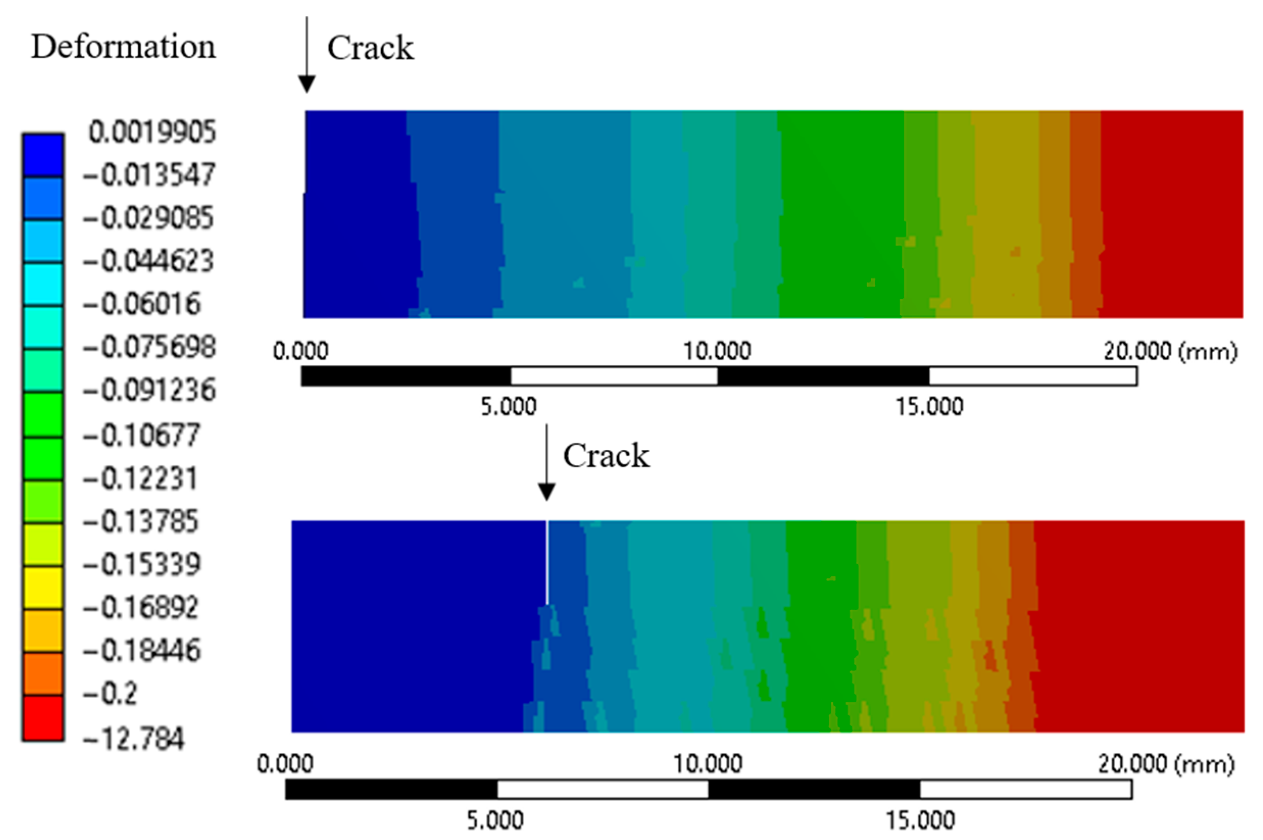The phenomenon is explained in detail in [30]. A suggestive representation of transverse displacements for a cantilever beam’s extreme segment fixed at the left end, for two crack positions, is given in Figure 1.

From the color scheme, one can observe in the above figure that, when the crack is positioned exactly at the fixed end (upper image), the deflection in the transverse direction is bigger at the slice located at 6 mm than the deflection of the beam with a crack located on that slice (bottom image). Subsequently, going toward the free end, the deflections increase faster for the beam with the crack located at 6 mm. Without a doubt, at the free end, this latter beam will achieve a bigger deflection.

A supplementary proof can be made with the results presented in

Table 1. Deflection at the free end for a cantilever beam affected by a transverse crack located at a distance x from the fixed end.

Crack Position [m]	δx (a) [mm] for a = 0.4 mm	δx (a) [mm] for a = 1 mm	δx (a) [mm] for a = 2 mm
x = 800	23.046	23.047	23.052
x = 600	23.048	23.057	23.097
x = 400	23.052	23.083	23.219
x = 200	23.059	23.134	23.455
x = 20	23.072	23.207	23.798
x = 0	23.061	23.124	23.401

. Here, we present the deflection under dead mass for a steel cantilever beam of length L = 1 m and cross-section $A=0.02\times 0.005$ m². The simulations were performed using ANSYS, for the crack positions and depths presented in Table 1. The chosen material is Structural Steel and the mesh is made using hexahedral elements of a maximum 1 mm edge size, thus obtaining a mesh of ~30,000 elements.

From Table 1, it is easy to observe that the deflection caused by a crack located at the fixed end is smaller than that when the crack is located at x = 20 mm and even x = 200 mm for all analyzed crack depths.

Taking into account the above, we can conclude that the severity to be considered when calculating the natural frequencies of the defective beams is the one estimated to be obtained at x = 0 on the curve constructed using the deflections determined for different positions of the defect. This theoretical deflection corresponds to that resulting from the deformation on both sides of the crack, which is impossible to obtain directly from FEA. Note that this severity does not apply when the crack is very close to the fixed end; here it indicates a bigger damage severity than it is in the real case.

Let us now introduce the pseudo-severity ${\gamma }_i(a,x)$, which reflects the effect of the severity weighted with the effect of the crack position. In fact, it reflects a decrease in the beam’s ability to store energy due to damage. This decrease, associated with the fact that energy distribution is in concordance with the modal curvature, permitted us to derive a function to calculate the natural frequency of a beam with a crack $f_{i-D}(a,x)$. The obtained mathematical relation is [31]

$$f_{i-D}(a,x)=f_{i-U}\left\{1-\gamma (a){\left[{\overline{{\mathsf{\varphi }}_i}}^{″}(x)\right]}^2\right\}$$

(3)

which makes use of the natural frequency of the intact beam $f_{i-U}$, the damage severity $\gamma (a)$, and the normalized mode shape curvature ${\overline{{\mathsf{\varphi }}_i}}^{″}(x)$. This relationship was successfully used to assess cracks [32], which proves its reliability.

From the right term in the parentheses of Equation (3), we can deduce the pseudo-severity as being

$${\gamma }_i(a,x)=\frac{\sqrt{{\delta }_i(a,x)}-\sqrt{{\delta }_u}}{\sqrt{{\delta }_i(a,x)}}=\frac{\sqrt{\delta (a,0)}-\sqrt{{\delta }_u}}{\sqrt{\delta (a,0)}}{\left[{\overline{{\mathsf{\varphi }}_i}}^{″}(x)\right]}^2=\gamma (a){\left[{\overline{{\mathsf{\varphi }}_i}}^{″}(x)\right]}^2$$

(4)

In Equation (4) we denoted the deflection of the beam with a crack of depth a that is located at the distance x from the fixed end as ${\delta }_i(a,x)$. One can observe that, dissimilar to the severity, the pseudo-severity severity depends on the vibration mode number i.

From Equation (4), we can deduce the mathematical relation for the deflection ${\delta }_1(a,x)$ of the cantilever beam under dead mass, when it has a crack located at the distance x from the free end, by performing the following steps:

$$\sqrt{{\delta }_1(a,x)}\sqrt{\delta (a,0)}-\sqrt{{\delta }_u}\sqrt{\delta (a,0)}=\sqrt{{\delta }_1(a,x)}\left(\sqrt{{\delta }_0}-\sqrt{{\delta }_u}\right){\left[{\overline{{\mathsf{\varphi }}_1}}^{″}(x)\right]}^2$$

(5)

$$\sqrt{{\delta }_1(a,x)}\left(\sqrt{\delta (a,0)}-\left(\sqrt{\delta (a,0)}-\sqrt{{\delta }_u}\right){\left[{\overline{{\mathsf{\varphi }}_1}}^{″}(x)\right]}^2\right)=\sqrt{{\delta }_u}\sqrt{\delta (a,0)}$$

(6)

$$\sqrt{{\delta }_1(a,x)}=\frac{\sqrt{{\delta }_u}\sqrt{\delta (a,0)}}{\sqrt{\delta (a,0)}-\left(\sqrt{\delta (a,0)}-\sqrt{{\delta }_u}\right){\left[{\overline{{\mathsf{\varphi }}_1}}^{″}(x)\right]}^2}$$

(7)

$${\delta }_1(a,x)=\frac{{\delta }_u\delta (a,0)}{{\left(\sqrt{\delta (a,0)}-\left(\sqrt{\delta (a,0)}-\sqrt{{\delta }_u}\right){\left[{\overline{{\mathsf{\varphi }}_1}}^{″}(x)\right]}^2\right)}^2}$$

(8)

If the crack is located at the fixed end, thus ${\overline{{\mathsf{\varphi }}_1}}^{″}(0)=1$, the deflection of the free beam end is ${\delta }_1(a,0)$. On the other hand, if the crack is located at the free end, thus ${\overline{{\mathsf{\varphi }}_1}}^{″}(L)=0$, the deflection of the free beam end is δ_u. This mathematical relation can be used to calculate the deflection at the free end of a cantilever beam with a crack. In this paper, we use the function given in Equation (8) to find the theoretical deflection ${\delta }_1(a,0)$ by an optimization algorithm.

3. Using the SHC to Estimate the Deflection When the Crack Is Located at the Fixed End

Stochastic Hill Climbing (SHC) is an optimization algorithm, which starts from a solution and expands it through incremental searches within a local area of the search space, using an objective function, until an optimum is found. This essentially makes it an ideal candidate in unimodal optimization problems, or after the application of a global optimization algorithm. Other similar types of algorithms, which aim to approximate a ‘good-enough’ solution instead of searching for a global best, exist. These include genetic algorithms, simulated annealing, random recursive search, and Tabu search. Most of these are applicable for a broad range of problems because they: (i) generally require little or no a priori knowledge, and (ii) can easily find an optimum solution by following local gradients using the objective function.

The SHC algorithm as used in this study considers as input three points $P_k(a,x_k)$ with k = 1…3. These points are the deflections of the beam at the free end when the crack is located at distances $x_1$, $x_2$ and $x_3$, found involving the FEA. In addition, we indicate the deflection of the intact beam derived by the means of FEA, which is $P_u$. The output consists of one point, which is the deflection of the beam at the free end $\delta (a,0)$ achieved when the crack is located at the fixed end. The steps performed when running the algorithm are:

• Generate an initial point.
• Evaluate the initial point.
• Take a step s.
• Evaluate candidate point.
• Check if we should keep the new point.

The objective function used to evaluate a candidate solution is given by

$$c(s)=\sqrt{{\displaystyle \sum _{i=1}^n{({\delta }_1^{*}(a,x_k)-P_k(a,x_k))}^2}}$$

(9)

In Equation (9), the points $P_k$ are the deflections found from the finite element analysis and ${\delta }_1(a,x_k)$ are the deflections calculated, for the locations $x_1$, $x_2$ and $x_3$, with the mathematical relation

$${\delta }_1^{*}(a,x_k)=\frac{\stackrel{⌢}{\delta }(a,0){\delta }_u}{{\left(\sqrt{\stackrel{⌢}{\delta }(a,0)}-\left(\sqrt{\stackrel{⌢}{\delta }(a,0)}-\sqrt{{\delta }_u}\right){\left[{\overline{{\mathsf{\varphi }}_1}}^{″}(x_k)\right]}^2\right)}^2}$$

(10)

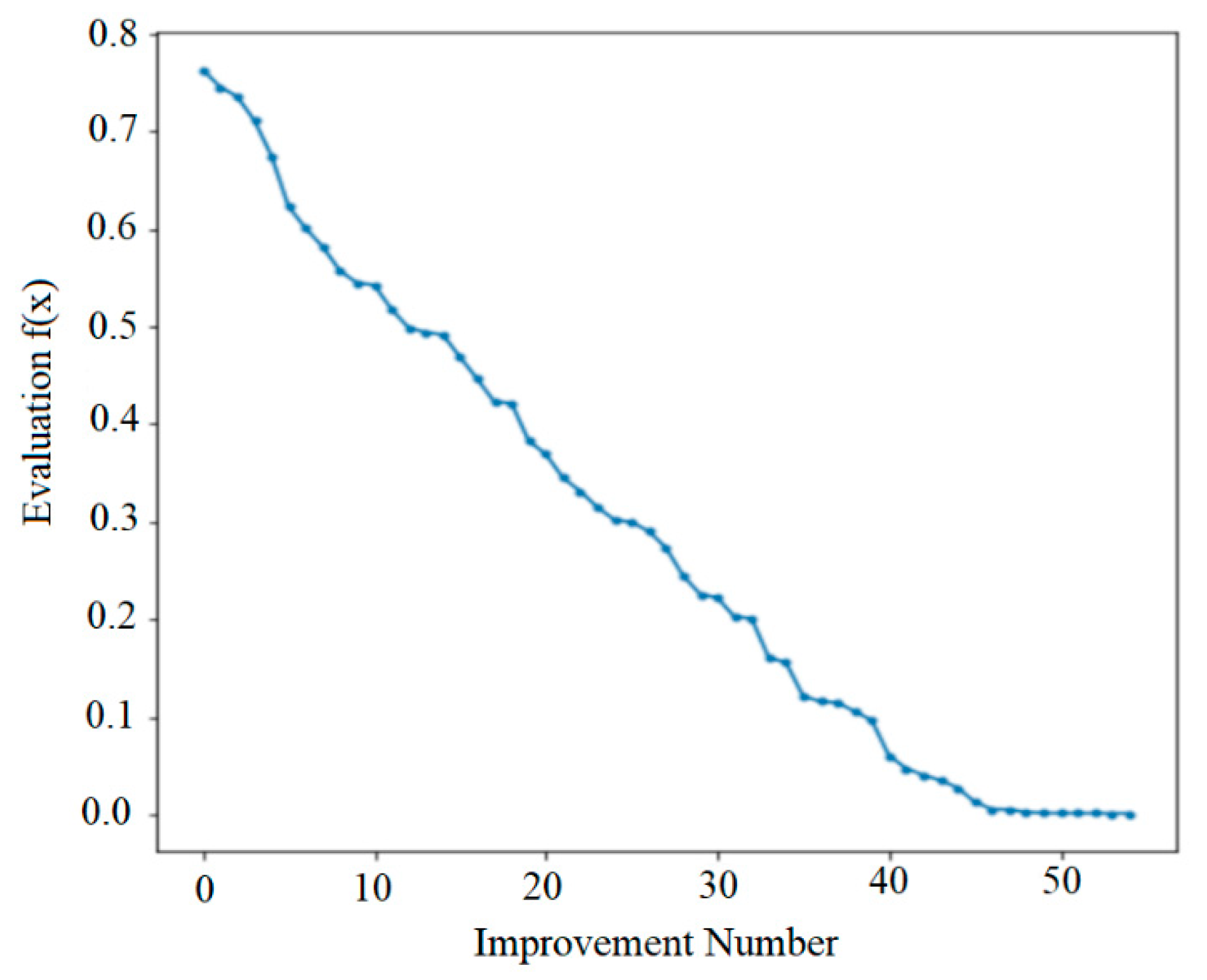
Here, $\stackrel{⌢}{\delta }(a,0)=s\cdot {\delta }_u$. The search process starts with considering s = 1, and its value is subsequently increased until c(s) achieves the lowest value possible. We exemplify here the case of a crack with a depth of 1 mm. Figure 2 shows the objective function evaluation for each improvement during the hill-climbing search. During the optimization process, we initially get big changes, and toward the end of the search, these changes become very small. After about 50 iterations the algorithm manages to converge on the optima.

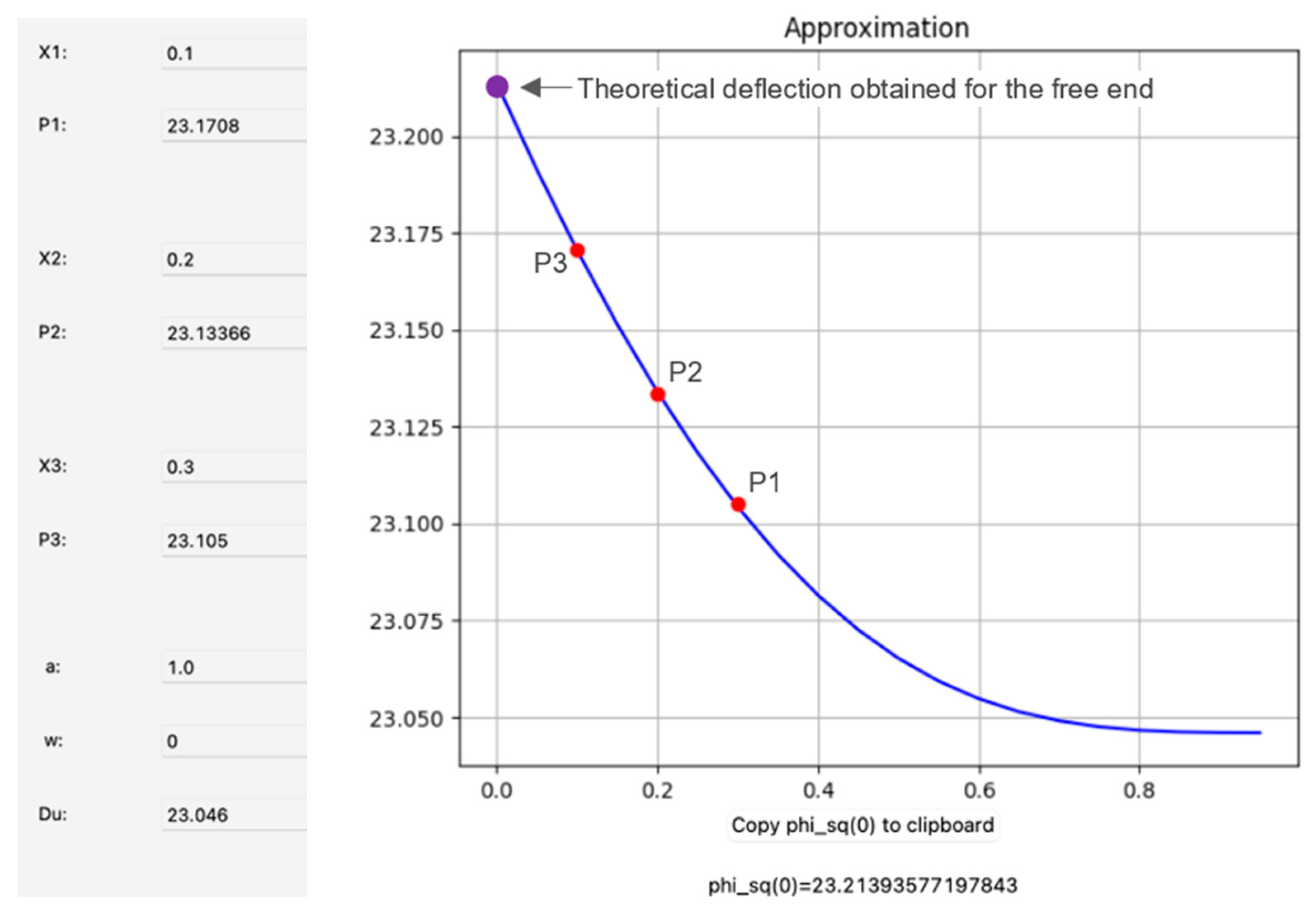
We have implemented our SHC algorithm in Python and created a basic user interface that allows us to easily estimate the deflections. Figure 3 shows the main window of the PySHC application.

In the developed Python application, it is necessary to input the damage depth a, the coordinates $x_k$/L, and the associated deflections $P_k(a,x_k)$ for the damaged beam $P_u$. After the input values are introduced, the algorithm determines the theoretical deflection obtained for the free end, when the crack is located at the fixed end. It is recommended that the chosen points are not too close.

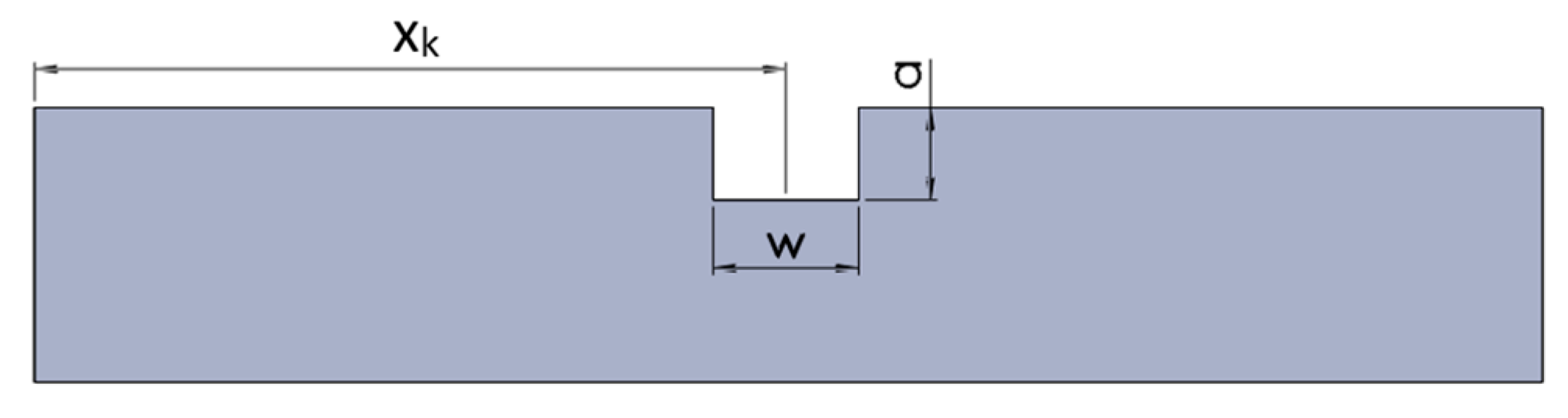
If the crack is an open one, as shown in Figure 4, in addition to the crack depth it is necessary to indicate the crack width w. This value is set to 0 by default in the application, indicating a closed crack. The input value for w should not exceed 5 mm, otherwise another damaged beam model is applicable [33,34].

4. Severity Curves Derived from the Calculated Damage Deflections

To determine the deflection caused by a crack that is located at the fixed end, using the described SHC algorithm, we have conducted FEM static simulations considering multiple damage scenarios. The beam considered in this study is like that presented in Section 2, thus it has the following dimensions: the length L = 1000 mm, the width B = 20 mm, and the thickness H = 5 mm. We also used the same material (Structural steel) and applied an identical simulation strategy.

The simulated transverse cracks are located at distances x₁ = 100 mm, x₂ = 200 mm, and x₃ = 300 mm from the fixed end. The crack depth starts from a = 0.2 mm and increases iteratively with a step Δa = 0.2 mm until the depth of 2 mm is achieved. The applied load was the dead weight, which produces a deflection in the transverse (vertical) direction. For each crack depth, we obtain from the FEM simulations three deflections for the beam’s free end, which are $P_1(a,100)$, $P_2(a,200)$ and $P_3(a,300)$. Using PySHC, we determine the theoretical deflection at the free end. The input data for the considered damage scenarios and the obtained deflection values are presented in

Table 2. Deflection at the free end for a cantilever beam with a crack that has the width w = 0 mm.

Damage Scenario	a [mm]	${\mathit{P}}_1(\mathit{a},100)$ [mm]	${\mathit{P}}_1(\mathit{a},200)$ [mm]	${\mathit{P}}_1(\mathit{a},300)$ [mm]	$\mathit{\delta }(\mathit{a},0)$ [mm]
1	0.2	23.05051	23.04915	23.04807	23.05203
2	0.4	23.06576	23.05987	23.05525	23.07250
3	0.6	23.09069	23.07740	23.06701	23.10592
4	0.8	23.12546	23.10178	23.08331	23.15287
5	1	23.17079	23.13365	23.10461	23.21369
6	1.2	23.22881	23.17437	23.13201	23.29203
7	1.4	23.30028	23.22457	23.16553	23.38859
8	1.6	23.38823	23.28624	23.20691	23.50768
9	1.8	23.49632	23.36178	23.25774	23.65446
10	2	23.62840	23.45544	23.32010	23.83521

for the closed crack and in

Table 3. Deflection at the free end for a cantilever beam with a crack that has the width w = 0.5 mm.

Damage Scenario	a [mm]	${\mathit{P}}_1(\mathit{a},100)$ [mm]	${\mathit{P}}_1(\mathit{a},200)$ [mm]	${\mathit{P}}_1(\mathit{a},300)$ [mm]	$\mathit{\delta }(\mathit{a},0)$ [mm]
11	0.2	23.05194	23.04741	23.04642	23.05161
12	0.4	23.07330	23.06490	23.05782	23.08210
13	0.6	23.10278	23.08532	23.07122	23.12135
14	0.8	23.14164	23.11220	23.08964	23.17352
15	1	23.19285	23.14674	23.11277	23.24136
16	1.2	23.25361	23.19128	23.14087	23.32423
17	1.4	23.32764	23.24303	23.17532	23.42406
18	1.6	23.42321	23.30889	23.22357	23.55420
19	1.8	23.54339	23.39505	23.27568	23.71710
20	2	23.68598	23.494056	23.34586	23.91250

,

Table 4. Deflection at the free end for a cantilever beam with a crack that has the width w = 1 mm.

Damage Scenario	a [mm]	${\mathit{P}}_1(\mathit{a},100)$ [mm]	${\mathit{P}}_1(\mathit{a},200)$ [mm]	${\mathit{P}}_1(\mathit{a},300)$ [mm]	$\mathit{\delta }(\mathit{a},0)$ [mm]
21	0.2	23.05194	23.04966	23.04784	23.05331
22	0.4	23.08282	23.07153	23.06199	23.09481
23	0.6	23.11673	23.09484	23.07764	23.13992
24	0.8	23.16138	23.12612	23.09826	23.19984
25	1	23.21792	23.16637	23.12452	23.27626
26	1.2	23.28805	23.21417	23.15746	23.37020
27	1.4	23.37186	23.27379	23.19689	23.48408
28	1.6	23.47622	23.34780	23.24623	23.62638
29	1.8	23.60532	23.44105	23.30606	23.80360
30	2	23.77482	23.55553	23.38395	24.03240

and

Table 5. Deflection at the free end for a cantilever beam with a crack that has the width w = 2 mm.

Damage Scenario	a [mm]	${\mathit{P}}_1(\mathit{a},100)$ [mm]	${\mathit{P}}_1(\mathit{a},200)$ [mm]	${\mathit{P}}_1(\mathit{a},300)$ [mm]	$\mathit{\delta }(\mathit{a},0)$ [mm]
31	0.2	23.05984	23.05340	23.05021	23.06241
32	0.4	23.10104	23.08376	23.06999	23.11881
33	0.6	23.14577	23.11485	23.09062	23.17848
34	0.8	23.20197	23.15414	23.05194	23.25396
35	1	23.27400	23.20445	23.14956	23.35081
36	1.2	23.36256	23.26645	23.19063	23.47044
37	1.4	23.47207	23.34311	23.24154	23.61869
38	1.6	23.60779	23.43813	23.30477	23.80337
39	1.8	23.77636	23.55631	23.38347	24.03397
40	2	23.98833	23.70488	23.48253	24.32582

for open cracks with different widths.

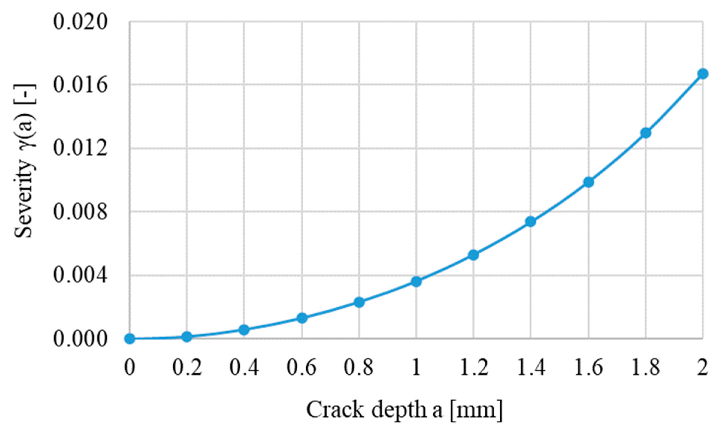
The main purpose of determining the theoretical deflections is to calculate the damage severities, which have a direct application in Structural Health Monitoring (SHM). We calculate the crack severities with Equation (1), the data utilized being $\delta (a,0)$ for the damaged beam and ${\delta }_u=23.046$ mm for the intact beam. The results obtained for the closed cracks are represented graphically in Figure 5.

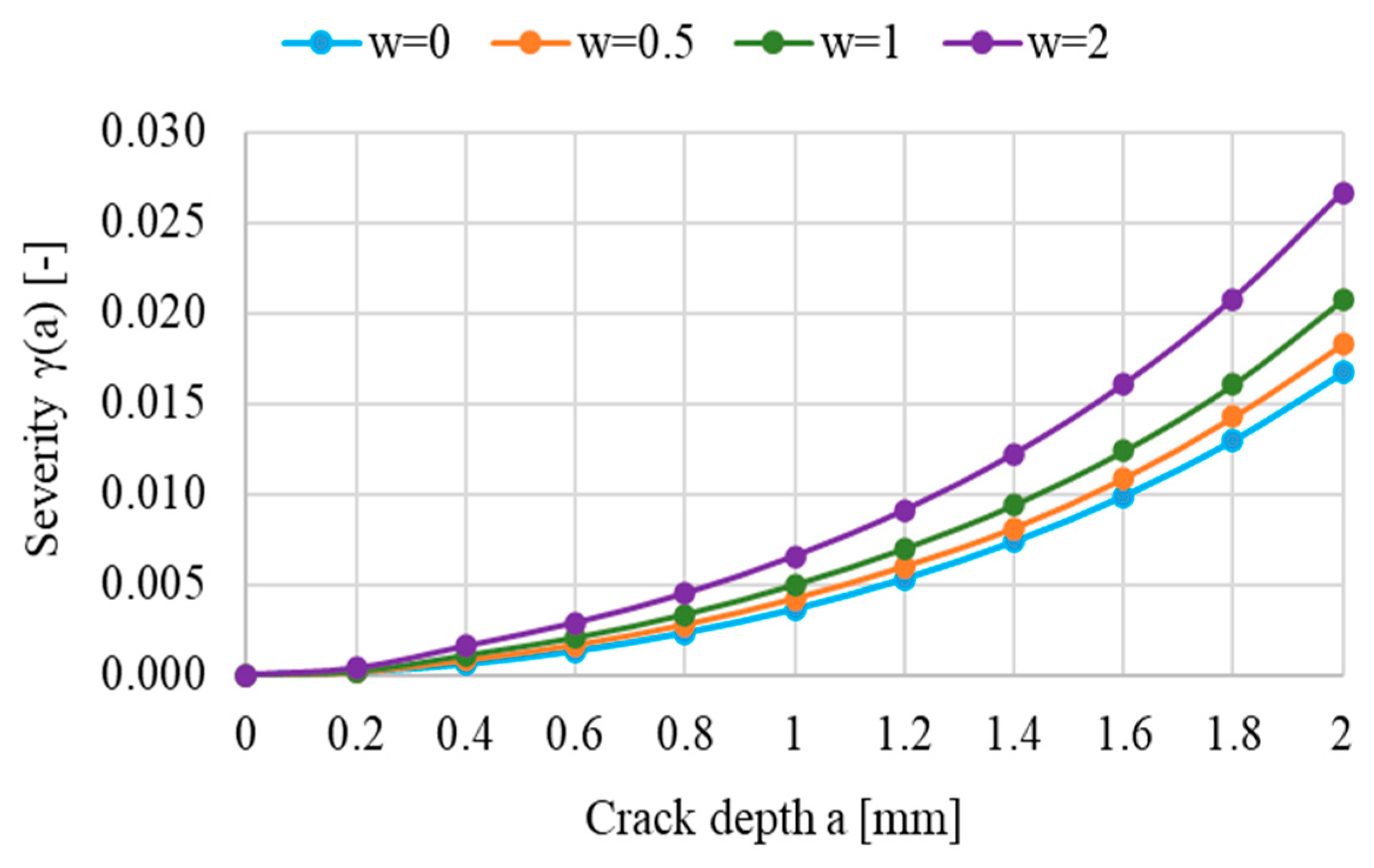
Furthermore, we determine the severity values for open cracks, considering the results presented in Table 3, Table 4 and Table 5. The severities calculated accordingly are depicted in Figure 6, along with the severities for the closed cracks for comparison. One can observe that an increase in the damage width has as a result an increase in the severity. However, the curves have the same shape.

5. Testing the Capacity of the Derived Severities to Accurately Predict Frequency Changes Due to Damage

In this section, we test the accuracy of the developed SHC algorithm and implicitly the analytical relation to calculate the deflection of beams with cracks. To this aim, we perform FEM simulation and laboratory experiments. Because the frequency changes are small, and even big errors can be overseen, we also compare the relative frequency shifts (RFS). The RFSs are frequency changes normalized by the natural frequencies of the intact beam and are calculated using the following mathematical relation [35]:

$$\Delta {\overline{f}}_{i-D}(a,x)=\frac{f_{i-U}-f_{i-D}(a,x)}{f_{i-U}}=\gamma (a){\left[{\overline{{\varphi }_i}}^{″}(x)\right]}^2$$

(11)

By normalization, the changes become more easily comparable, and a better assessment of the method’s reliability is possible. Moreover, these RFSs are used in damage detection, so it is important to evaluate if analytically deduced RFSs can be used to construct reliable databases that contain the structural response for a multitude of damage scenarios.

We can extract the severity from Equation (11), resulting in

$$\gamma (a)=\frac{1}{{\left[{\overline{{\varphi }_i}}^{″}(x)\right]}^2}\frac{f_{i-U}-f_{i-D}(a,x)}{f_{i-U}}$$

(12)

Testing is made by comparing the severity obtained from static tests with the RFS obtained from dynamic tests made in the laboratory. From the static tests, made through FEM simulations, we obtain the deflections and calculate the severity with Equation (1). From the dynamic tests, made involving the FEM or laboratory experiments, we obtain the frequencies of the beam in the intact and damaged state. In addition, we can calculate the normalized modal curvature ${\overline{{\varphi }_i}}^{″}(x)$, and eventually the right term in Equation (12), which has also the meaning of the severity. Now, by comparing the two results, we can conclude if these fit and if the prediction of frequency changes can be reliably made with Equation (3). In this mathematical relation, we consider the measured frequency of the intact real beam and the severity deduced from the deflections of the beam under its own weight.

5.1. Tests Performed with FEA

Damage detection using modal parameters requires accurate algorithms to detect the slightest frequency changes in structures. For determining the accuracy of the described method used for detecting transverse cracks, we have performed FEM modal simulations using the ANSYS software for the same cantilever beam described in Section 2. The beam is successively affected by closed and open transverse cracks with different depths and located in different slices of the beam.

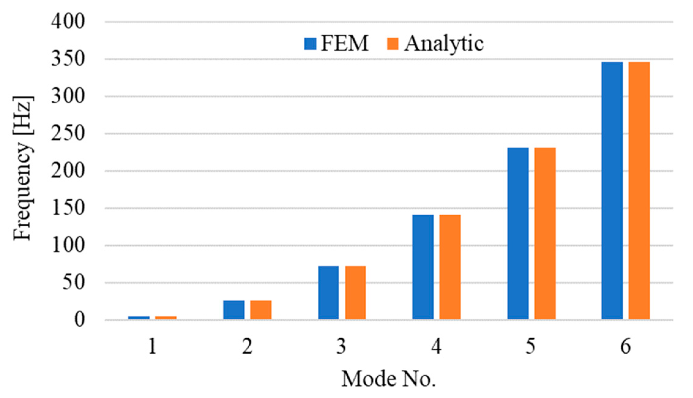
As a first example, we present in Figure 7 the natural frequencies obtained from simulation and with Equation (3) for the beam with a transverse crack that has the parameters: x = 604 mm, a = 1 mm, and w = 0 mm. When using the analytical approach, we calculate the frequencies with Equation (3) in which we consider the measured frequency of the intact beam and the severity deduced from the deflections achieved by static analysis.

At a first look, the frequencies in Figure 7 fit, but it is difficult to evaluate the accuracy of the method. However, one can observe that the differences between the natural frequencies obtained involving the analytical method and the FEM results are small.

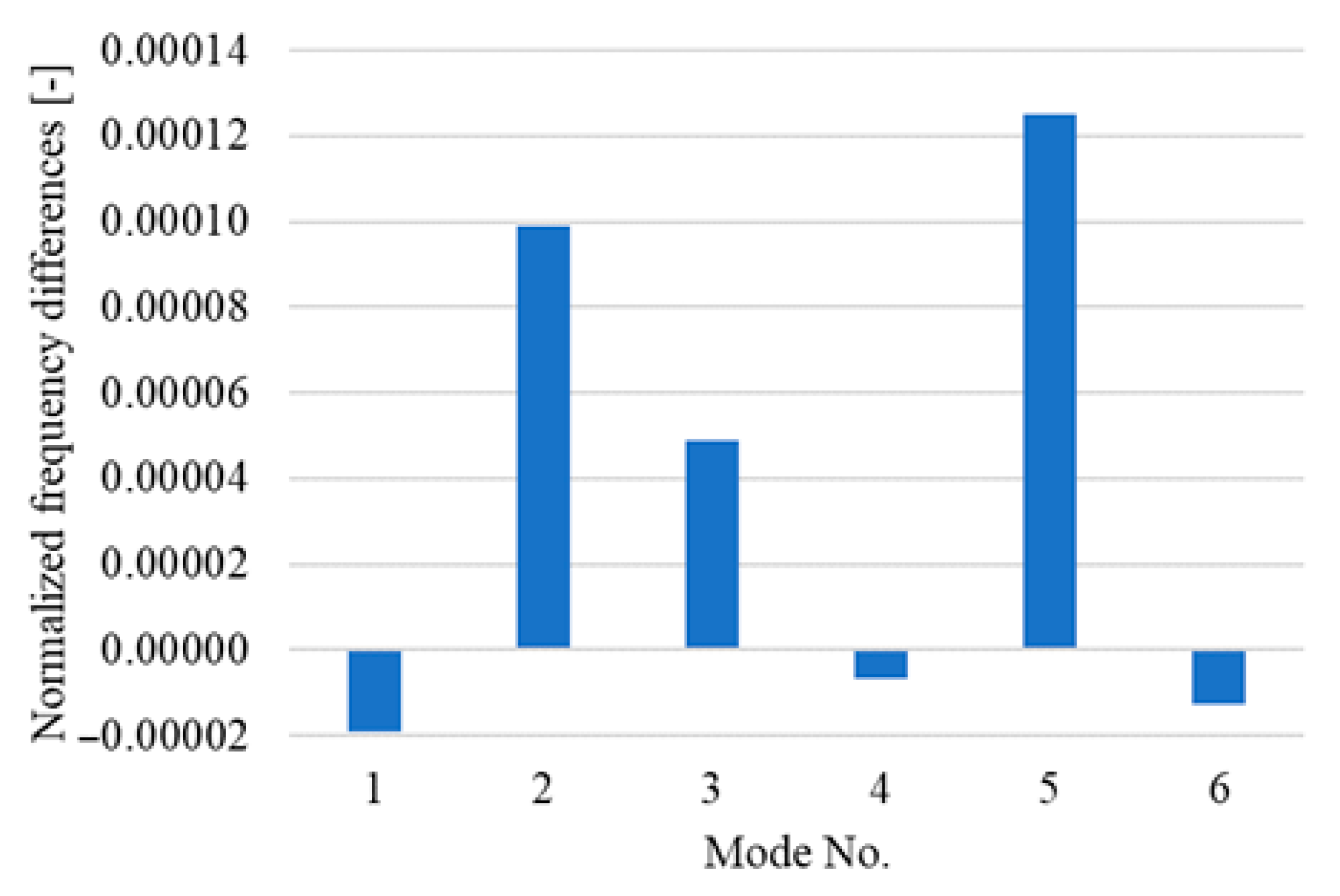
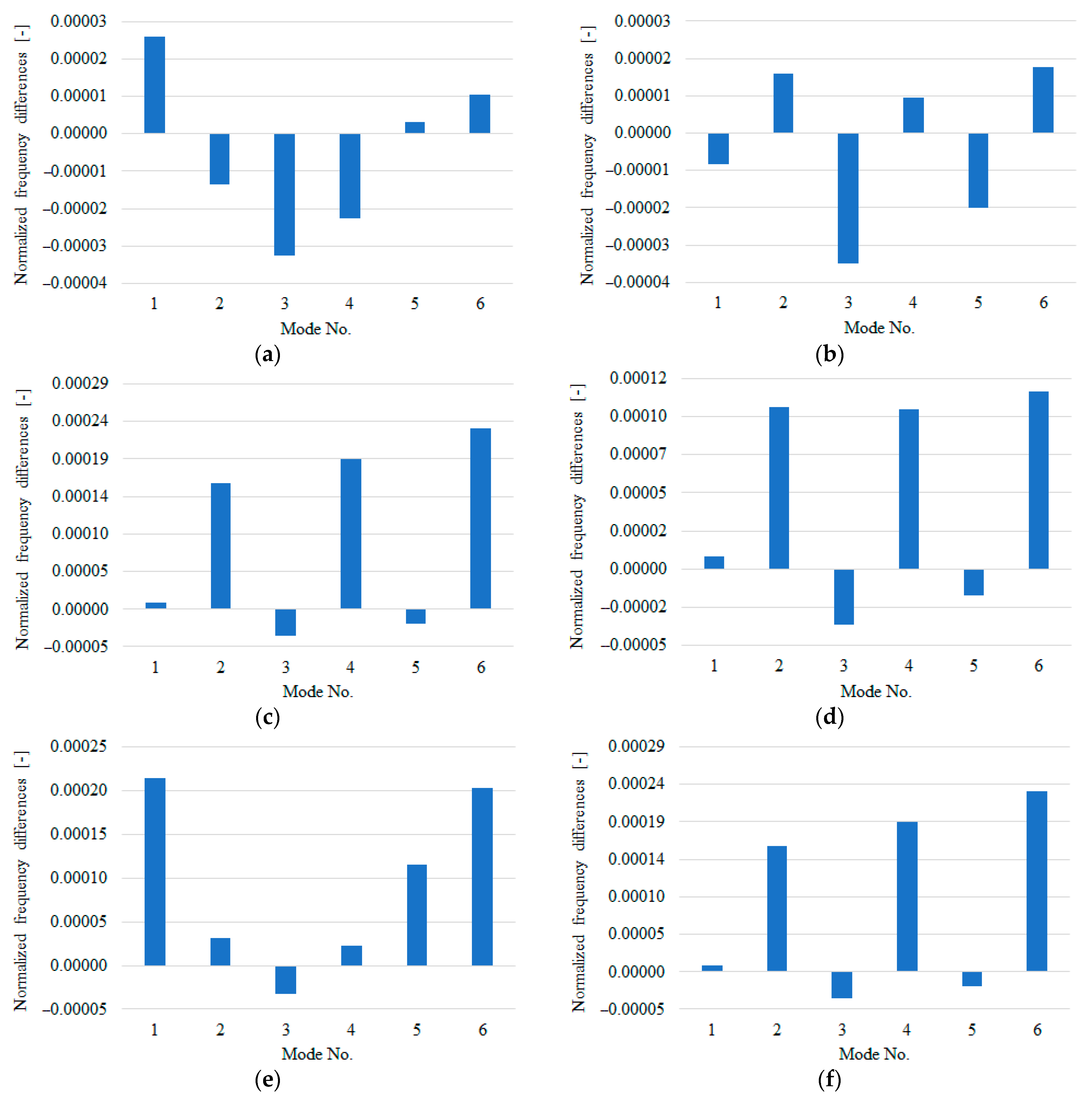
To trace a relevant conclusion, we represent in Figure 8 the difference between the predicted frequencies and those obtained from simulation. Before being represented, the differences are normalized, according to the mathematical relation

$$\epsilon =\frac{f_{i-D}(FEM)-f_{i-D}(a,x)}{f_{i-U}}$$

(13)

One can observe that absolute normalized differences are extremely small, between −0.000019 and +0.000125. Because the frequency differences are normalized, the error does not increase with the mode number. By calculating the normalized differences for more damage scenarios, we found out that the errors are comparable or smaller. This proves that the results obtained with the DS-SHC method are reliable.

A second example considers also closed cracks, thus w = 0 mm. The damage scenarios are defined in ANSYS, for three crack depths a = 0.2, 1, and 1.6 mm. For each crack depth, the position of the crack is x = 125 mm and x = 489 mm, respectively. After we defined the damage scenarios, we determined the severity γ(a)_FEM using relation 12 for the first six weak-axis vibration modes. Relative to the crack’s main dimensions, a, x, and w, the damage scenarios are noted as C(a,x,w). The severity values γ(a)_FEM are compared, in Figure 9, with the calculated ones γ(a).

A third example considers open cracks. We performed FEM simulations for defined damage scenarios that involve cracks with widths w of 0.5, 1, and 2 mm. The results for all damage scenarios are presented in [36].

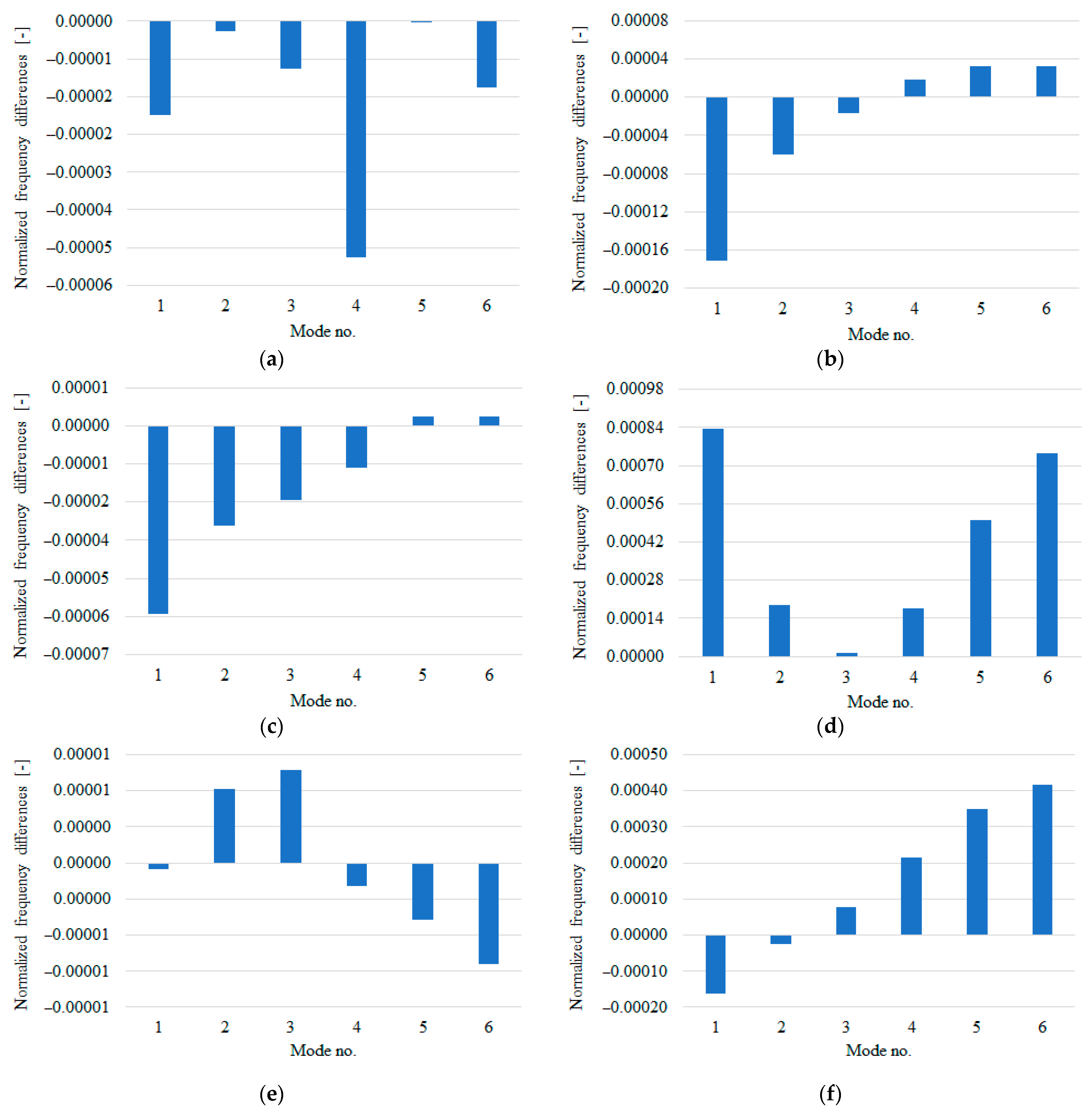
For a part of the open damage scenarios, noted as C(a,x,w), the normalized differences calculated between the natural frequencies determined analytically and employing FEM are presented in Figure 10.

5.2. Tests Performed Involving Laboratory Experiments

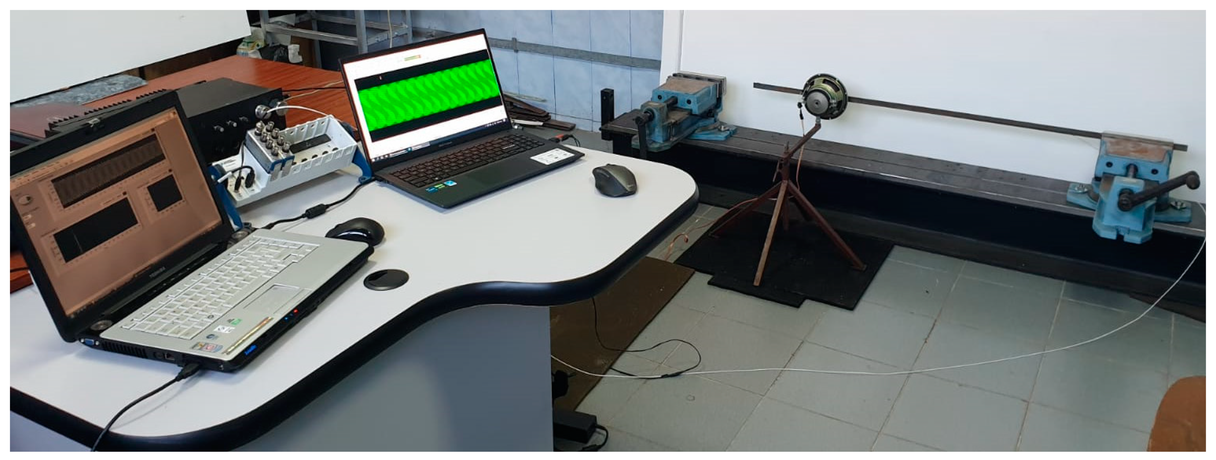
To prove the accuracy of the developed algorithm, we also conducted laboratory studies on steel cantilever beams affected by transverse cracks of known location, depth, and width. The tests consist of measuring the natural frequencies in the intact and damaged state. Because the accuracy of RFS calculated with Equation (11) is relevant for damage detection, in this section we compare these RFS with those obtained from measurements. The laboratory setup consists of a rigid structure including a vise in which the beam is fastened, an excitation device, and the data acquisition system. The experimental setup is presented in Figure 11 and described in detail in [27].

The excitation system involves a speaker and amplifier which are controlled using AudioDope software. The beam is excited at specific frequencies, and the vibration response is acquired. To acquire the signals, we use a data acquisition system consisting of a Kistler 8772 accelerometer which transmits the signal through the analog-to-digital conversion module NI9234 to the compact chassis NIcDAQ-9175. This module is connected to a second laptop, on which the LabVIEW software is installed. The acceleration signal is acquired and is subsequently processed to extract the natural frequencies with high accuracy using the procedure described in [37,38]. The Python code implementing the procedure is available in [39].

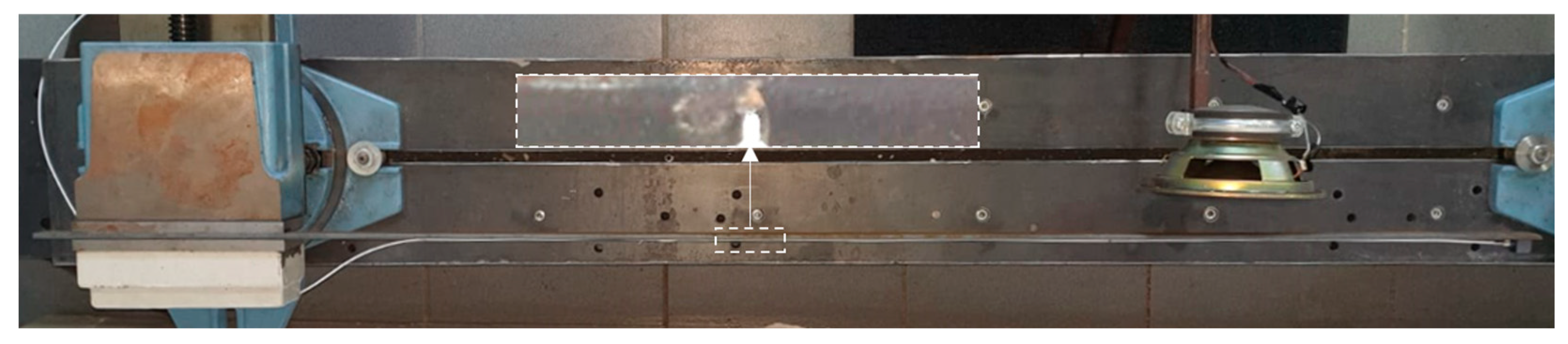
The experimental study was carried out on four S355 JR steel cantilever beams of dimensions 1 × 0.05 × 0.005 m, at first in an intact state and later in a damaged state, by generating transverse cracks of width w = 2 mm by saw cutting. One end of the beams is fixed in a vise (see Figure 12).

At least five natural frequency readings were made for each test and the arithmetic mean was considered. For each reading, the first six natural frequencies of the beam were extracted, and the obtained values are listed and compared with the natural frequencies obtained from FEM in

Table 6. Obtained natural frequencies for the undamaged test beams.

Beam nr.	Measured Natural Frequencies [Hz]
	Mode 1	Mode 2	Mode 3	Mode 4	Mode 5	Mode 6
Beam 1	4.060	25.439	71.426	139.902	231.038	344.750
Beam 2	4.052	25.448	71.213	139.342	230.295	343.254
Beam 3	4.011	25.237	71.102	138.575	229.421	342.904
Beam 4	4.044	25.482	71.287	139.420	228.528	344.177

. From the compared values the small differences can be observed.

A transverse open crack was generated on each beam analyzed above, thus resulting, for a single beam, six natural frequency values corresponding to the six transverse vibration modes.

We present in

Table 7. Obtained natural frequencies for the damaged beams.

Damage Scenario	a [mm]	x [mm]	w [mm]	γ(a) [-]	Measured Natural Frequencies [Hz]
					Mode 1	Mode 2	Mode 3	Mode 4	Mode 5	Mode 6
Beam 1	0.8	310	2	0.004503233	4.054	25.425	71.286	139.832	230.933	343.984
Beam 2	1.2	587	2	0.009104778	4.051	25.356	71.071	139.131	229.403	343.204
Beam 3	1.2	395	2	0.009104778	4.003	25.166	71.002	138.496	228.555	342.860
Beam 4	2	795	2	0.026682373	4.044	25.431	70.553	137.544	226.899	343.963

the crack dimensions for each damage scenario and the measured natural frequencies. In this table, we also included the severities for the four cracks, derived using the method described in the current research.

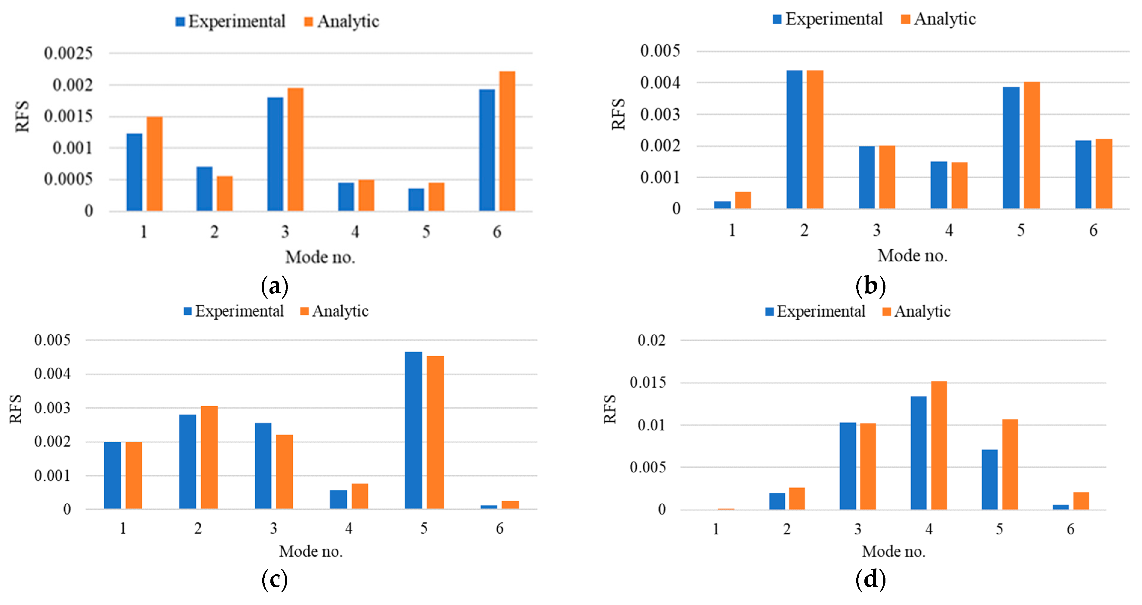
We calculate now the RFSs with the frequencies taken from Table 6 and Table 7, which are found from experiments. To this aim we use Equation (11). We also calculate the RFSs analytically (see Section 2). In this case, the input data consists of the deflections obtained from FE simulations; these permit calculation of the severity with Equation (1). With the calculated severity we find the frequency drop with Equation (3) and, finally, the RFSs with Equation (11). The comparison between the RFSs obtained with experimental results and those calculated is presented in Figure 13.

From the diagrams represented in this figure, it can be observed that there is a good fit between the compared values. Note that once the severity curves are known and plotted as in Figure 6, the severity can be easily determined for any damage depth. Thus, the FE simulations are no longer required when the procedure is applied.

By using the method described in the current paper, by employing Equation (11), we have generated training data for developing a damage detection neural network similar to the one presented in [13]. The training data consist of the RFS values for the six transverse vibration modes. After the network was trained, we successfully determined the position and depth of the cracks for the four experimental cases by considering the RFS values. The errors obtained are presented in

Table 8. Predicted locations and depths of the damage.

Damage Scenario	x [mm]	a [mm]	w [mm]	ANN Predicted Values
				x [mm]	εx [%]	a [mm]	εa [mm]
Beam 1	310	0.8	2	321.07	1.107	1.06	0.26
Beam 2	587	1.2	2	598.01	1.101	1.49	0.29
Beam 3	395	1.2	2	394.41	−0.059	1.38	0.18
Beam 4	795	2	2	791.09	−0.391	1.94	−0.06

.

The results prove the accuracy of the applied method for determining the position and severity of transverse cracks.

6. Conclusions

The paper presents the DS-SHC method, which can determine the severity of a crack involving just four static tests, one for the intact beam and three for the beam affected by a defect for which the positions are changed successively. From the tests performed for the defective beam, deflection is determined at the free end of a cantilever. Subsequently, using the SHC algorithm, the theoretical deflection that occurs when the crack is at the fixed end is determined. The matching of the three points is carried out on the function proposed in this paper, which expresses the deflection with the crack position. This theoretical deflection is different from the deflection achieved when the crack is at the fixed end because of constructive reasons. Finally, the severity is calculated from the capability of the beam with a crack to store energy, which is reflected by the increase of deflection at the free end.

To prove the reliability of the DS-SHC method, we compared the frequencies of the damaged beam calculated with the severity derived by employing the theoretical deflection with the frequencies obtained for the damaged beam using the FEM. The normalized differences between these frequencies are extremely low, less than ±0.001, which proves the reliability of the DS-SHC method. Moreover, we demonstrated here that the theoretical deflection for the damaged beam has to be considered when calculating the damage severity.

An additional check was made to find out whether the prediction of the frequency changes made with the severity calculated based on the theoretical deflection permits assessing the damage. In the laboratory experiments we conducted, we were able to localize the damage with high accuracy, the errors being less than 1.1%. The damage depth was also found with high accuracy; the difference between the depth of the generated damage and the prediction is smaller than 0.3 mm.

In the next studies, we will focus on finding whether the severity derived for the cantilever beam can be used for beams with other boundary conditions, and how accurate the severities for structures with other shapes of the cross-section can be determined.