
Semantic Segmentation of Agricultural Images Based on Style Transfer Using Conditional and Unconditional Generative Adversarial Networks

Abstract
:1. Introduction
2. Related Studies
3. Proposed Framework
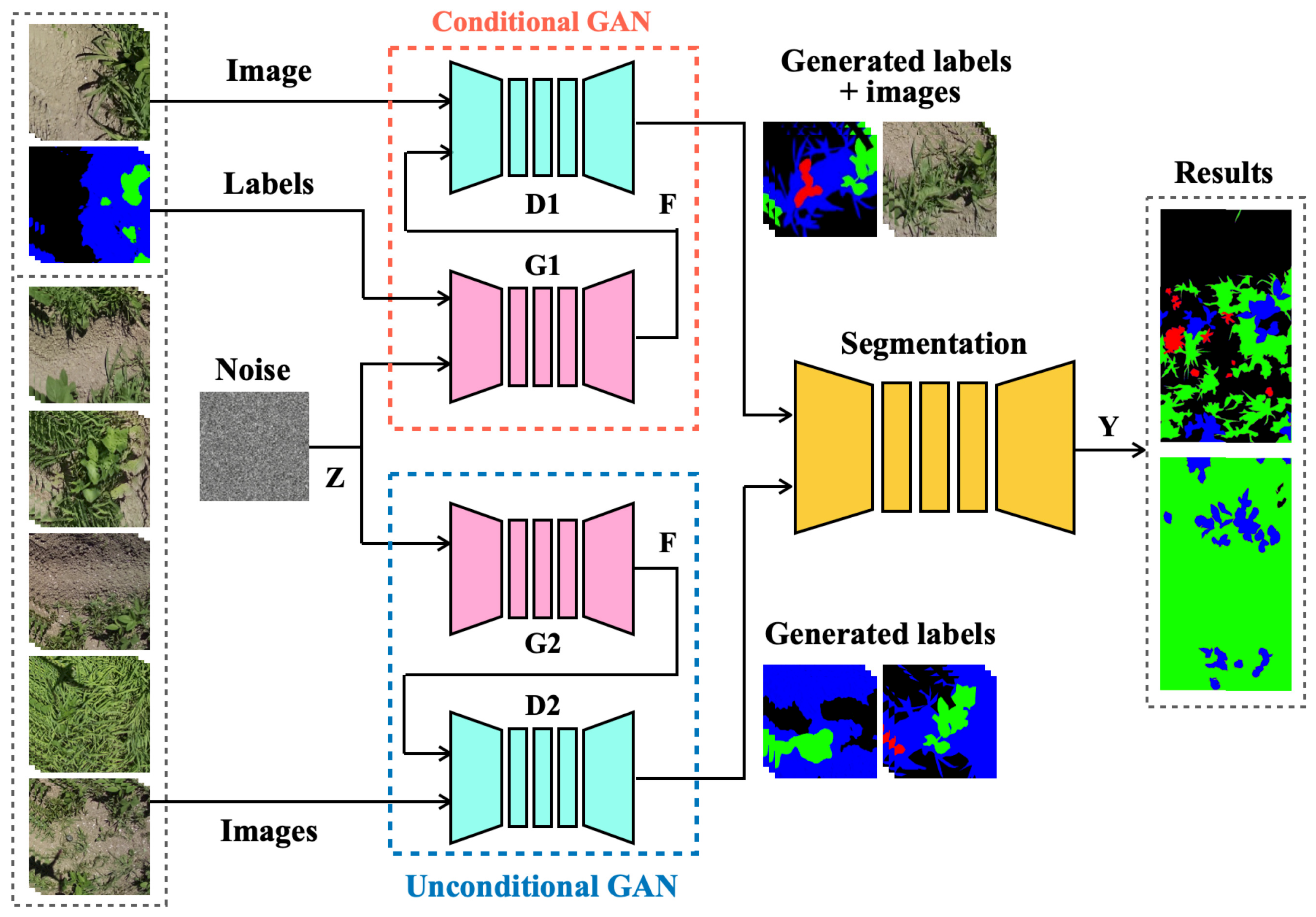
3.1. Overall Network Architecture
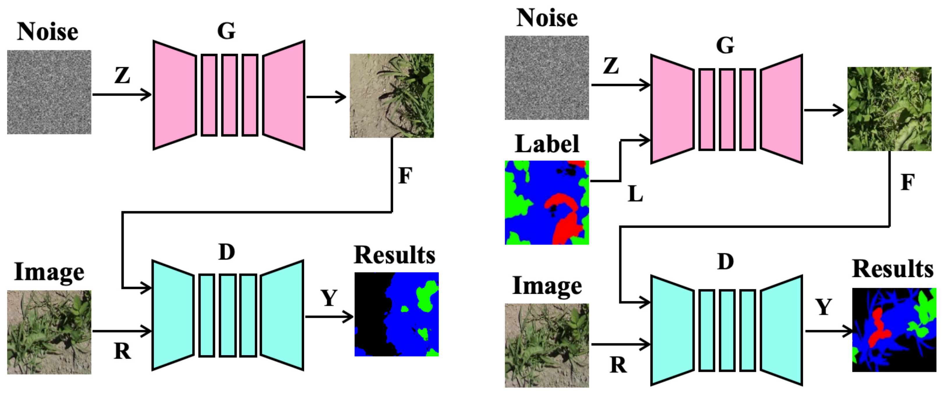
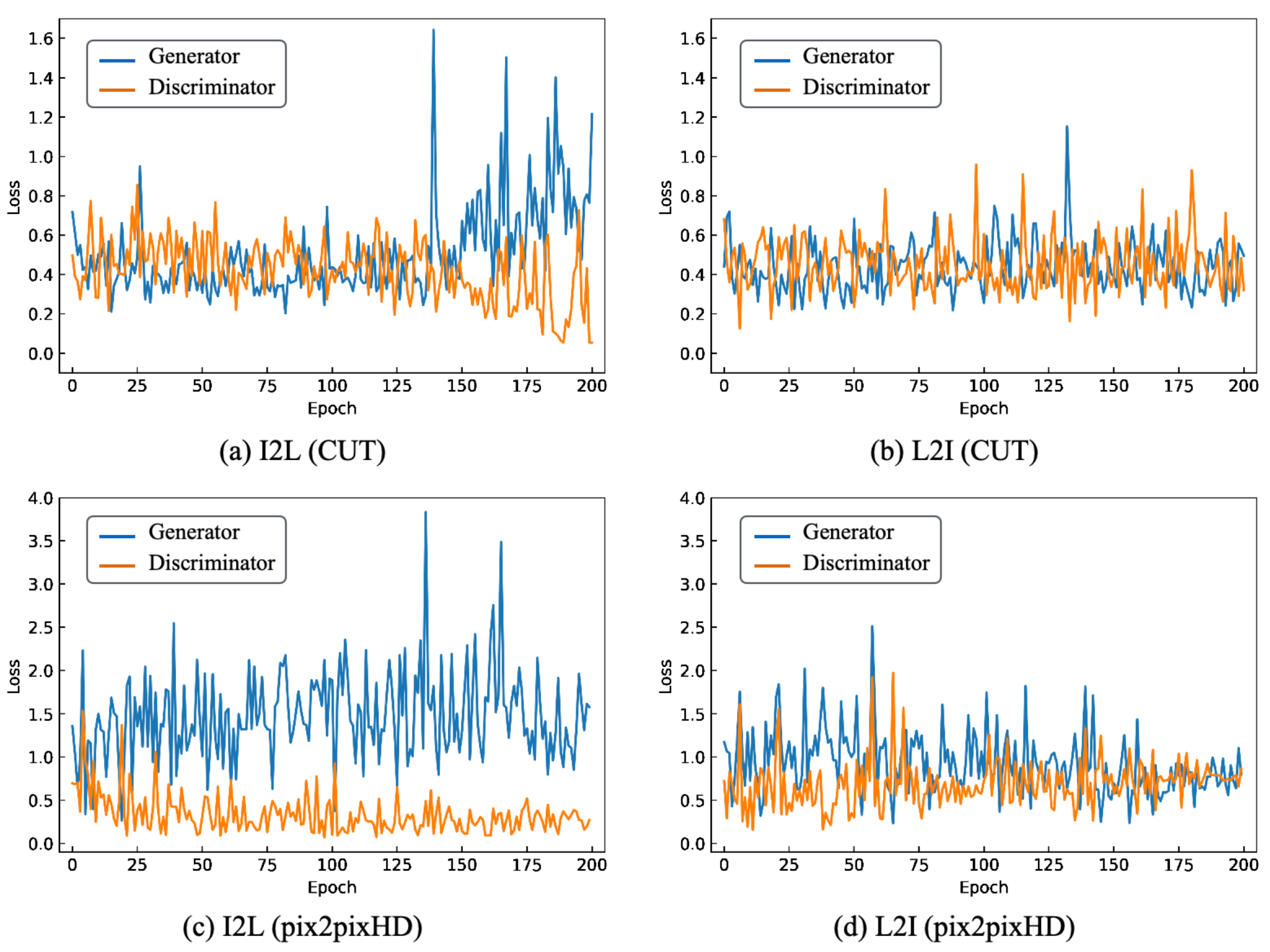
3.2. GAN
3.2.1. Unconditional GAN
3.2.2. Conditional GAN
3.3. Semantic Segmentation
4. Requirements
4.1. Benchmark Datasets
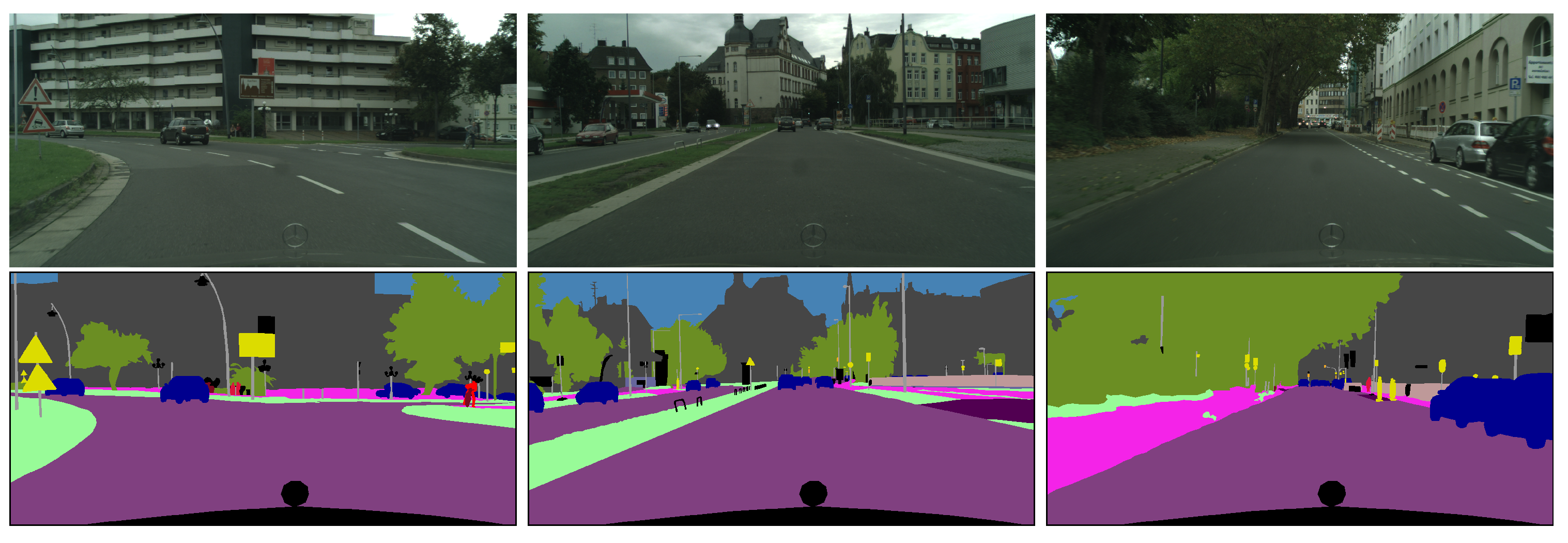
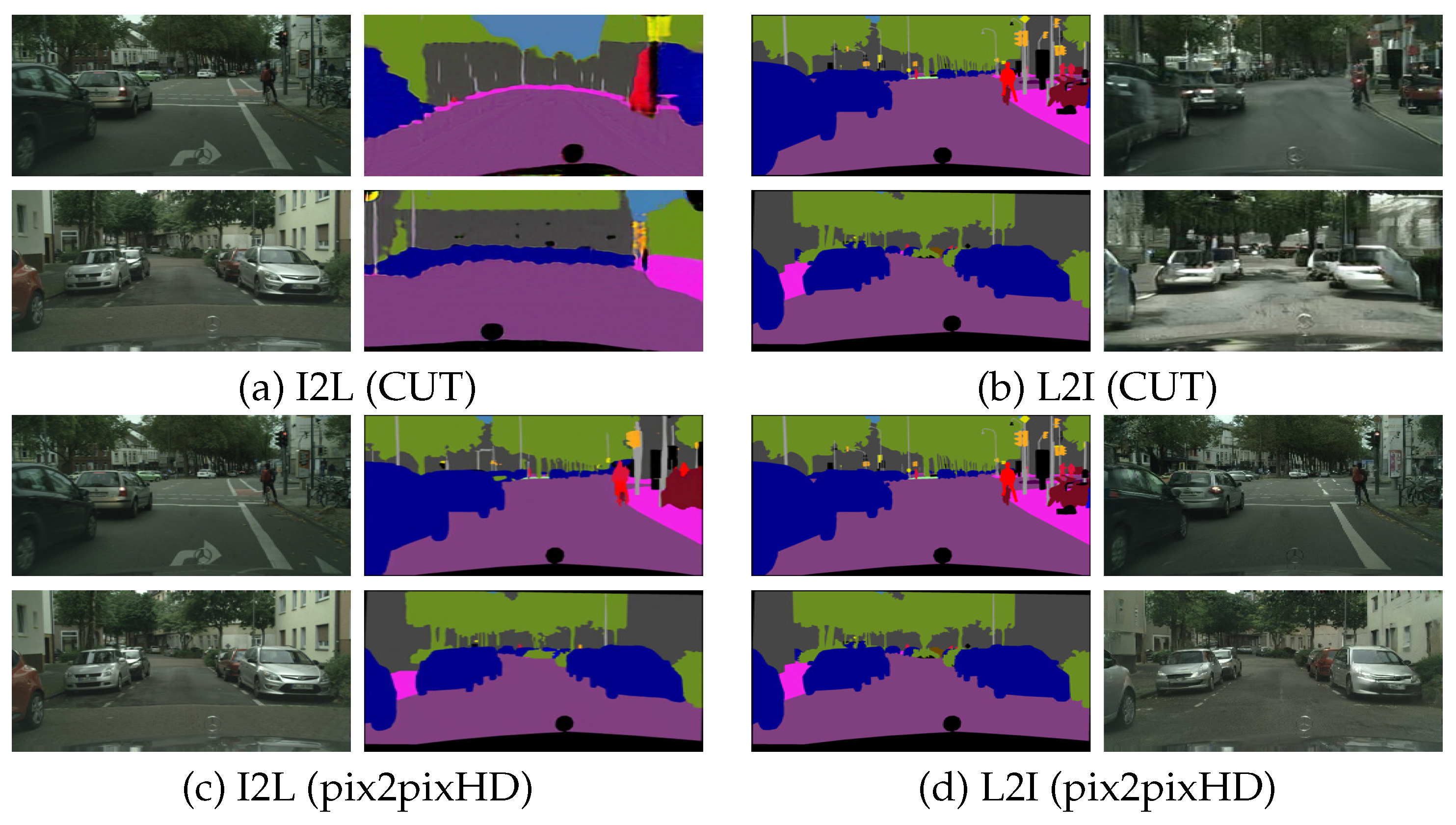
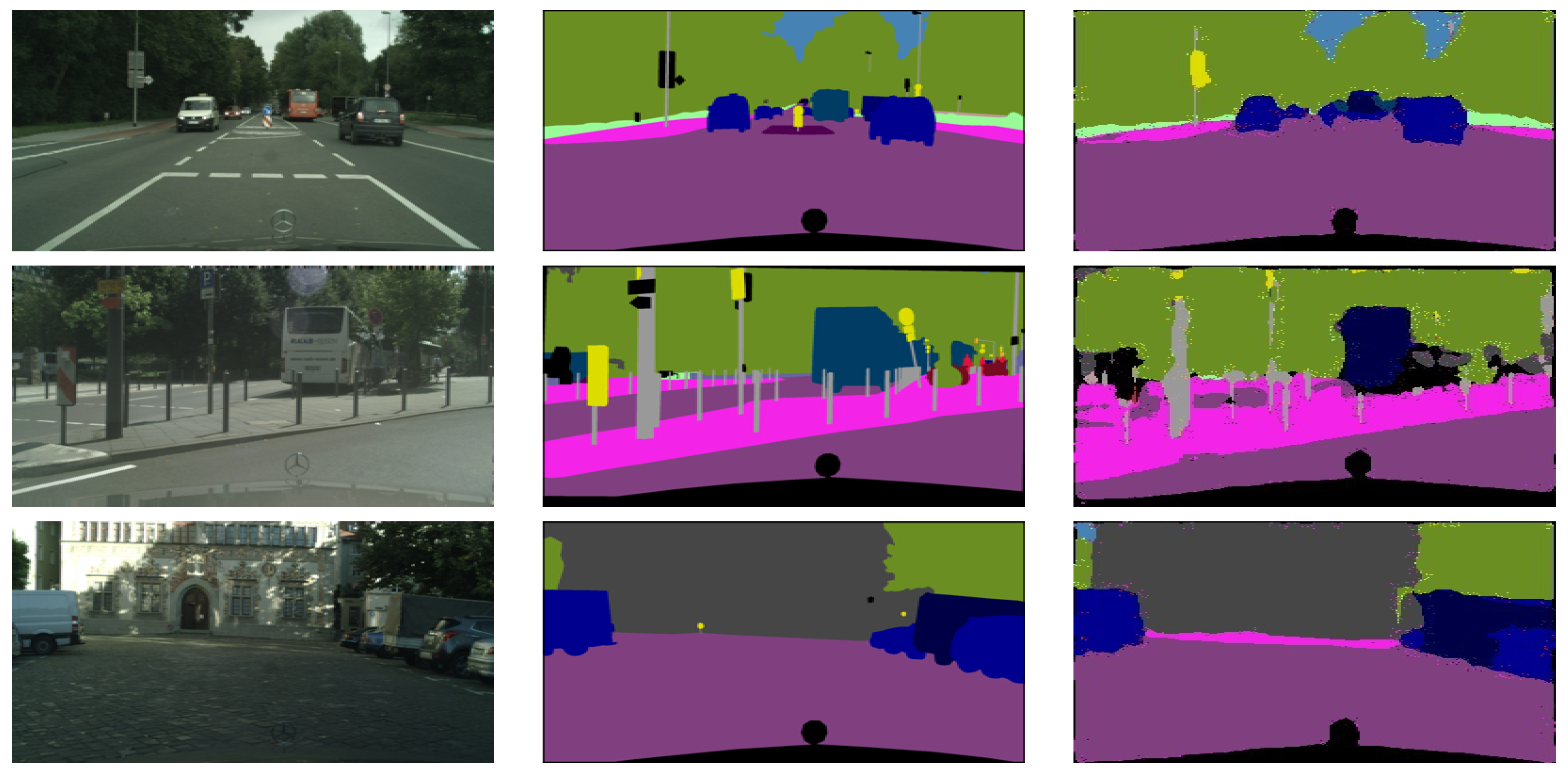
4.1.1. Cityscapes
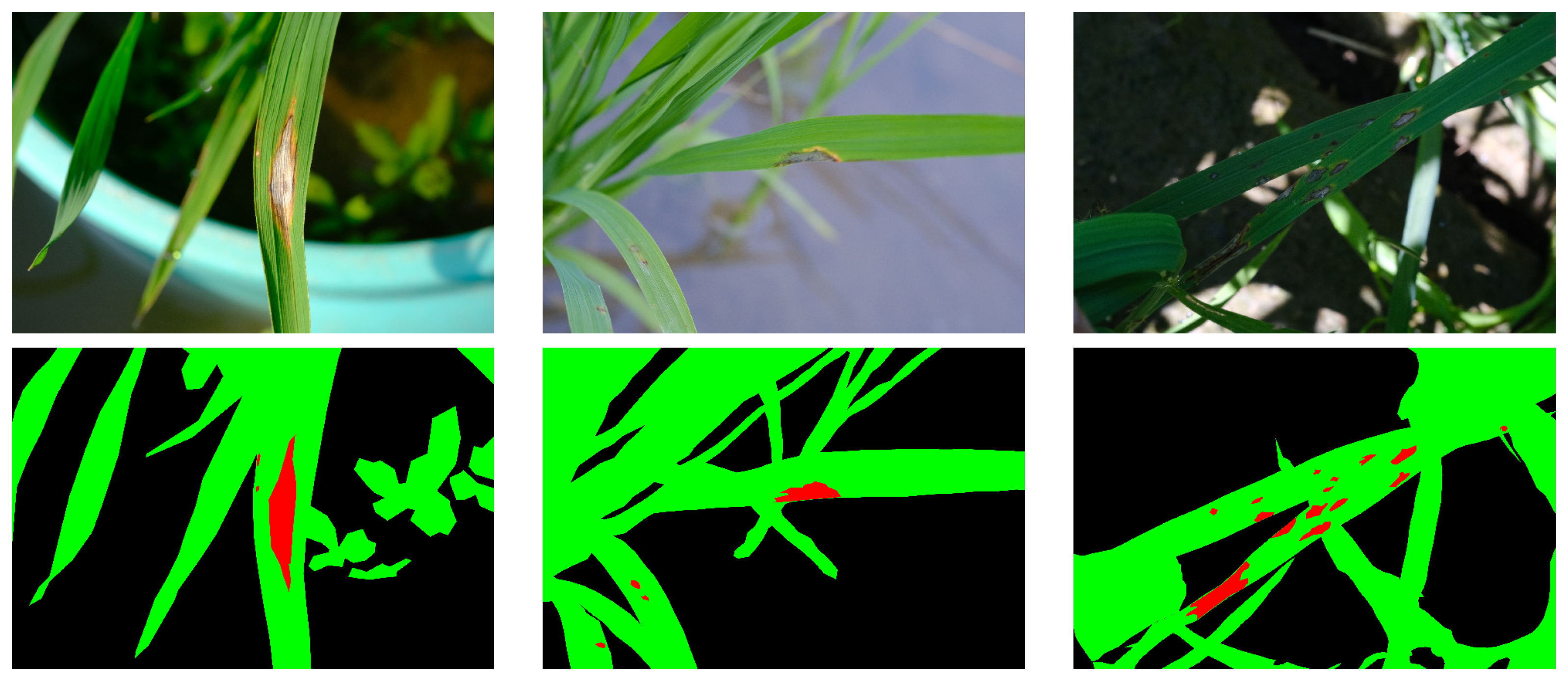
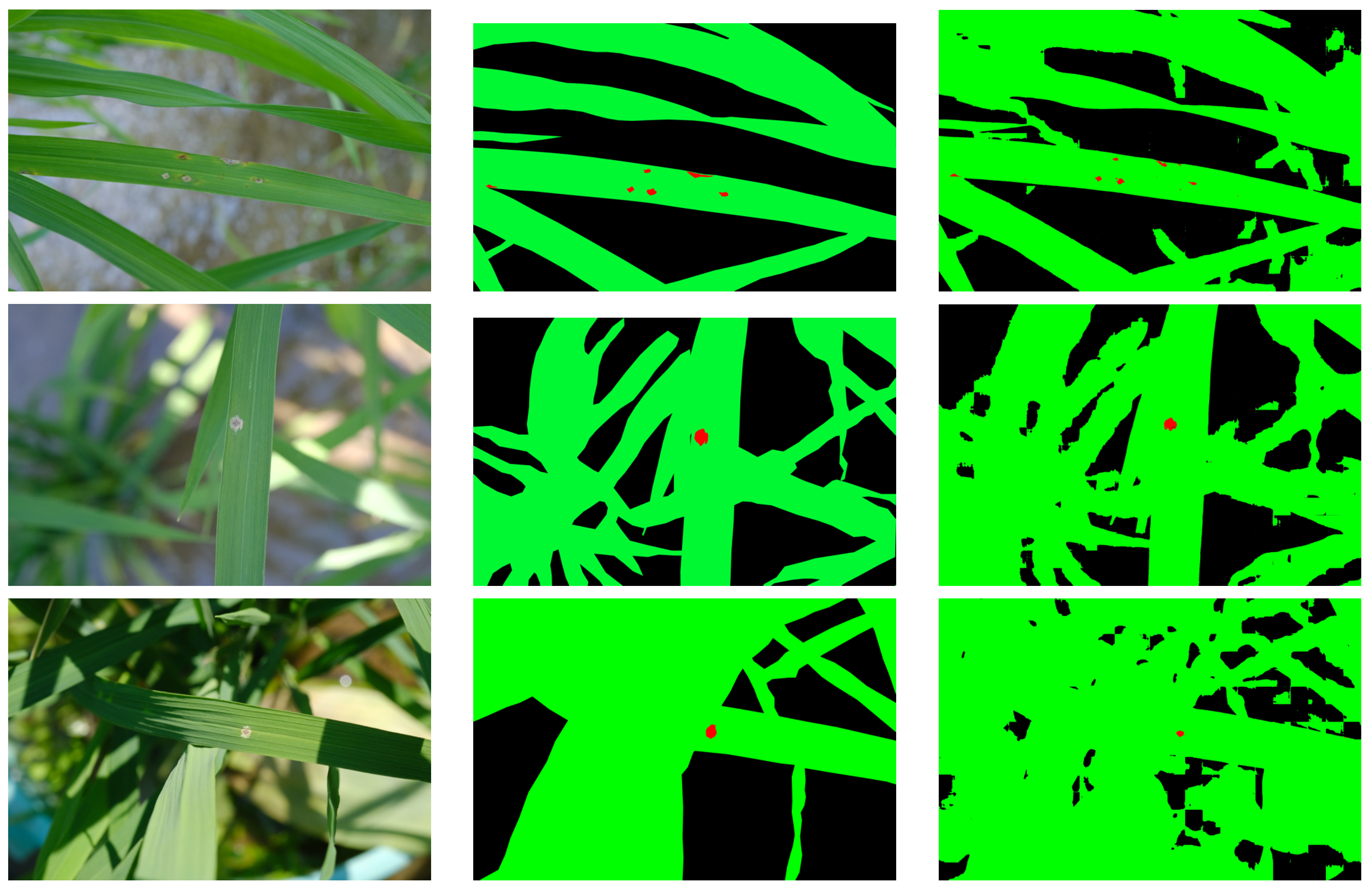
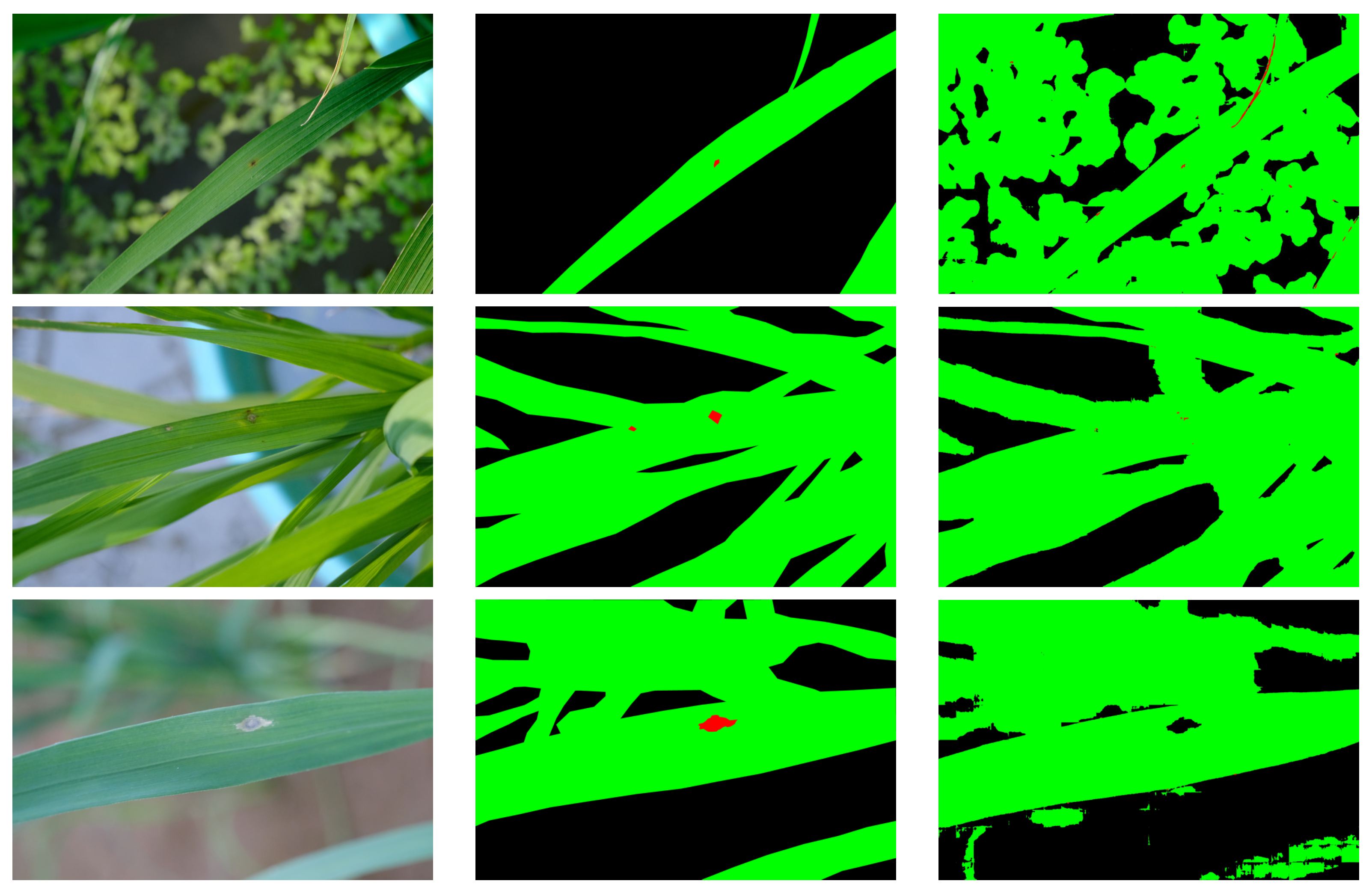
4.1.2. Rice Blast
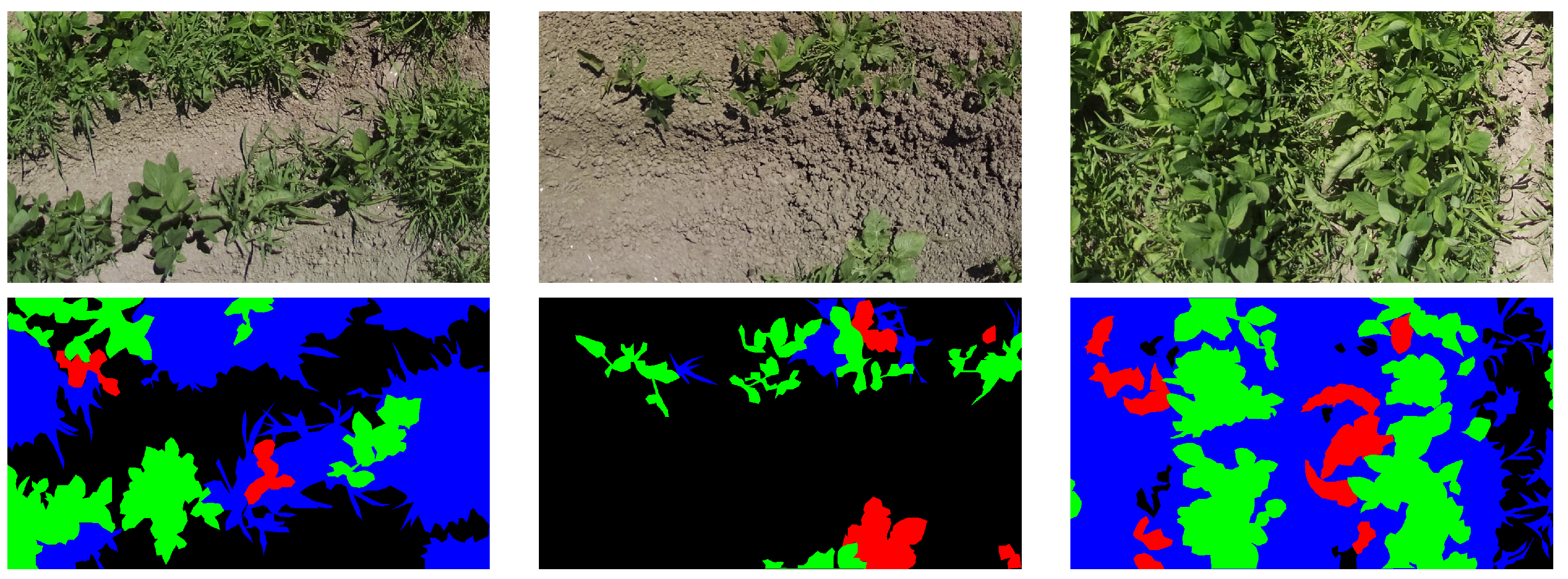
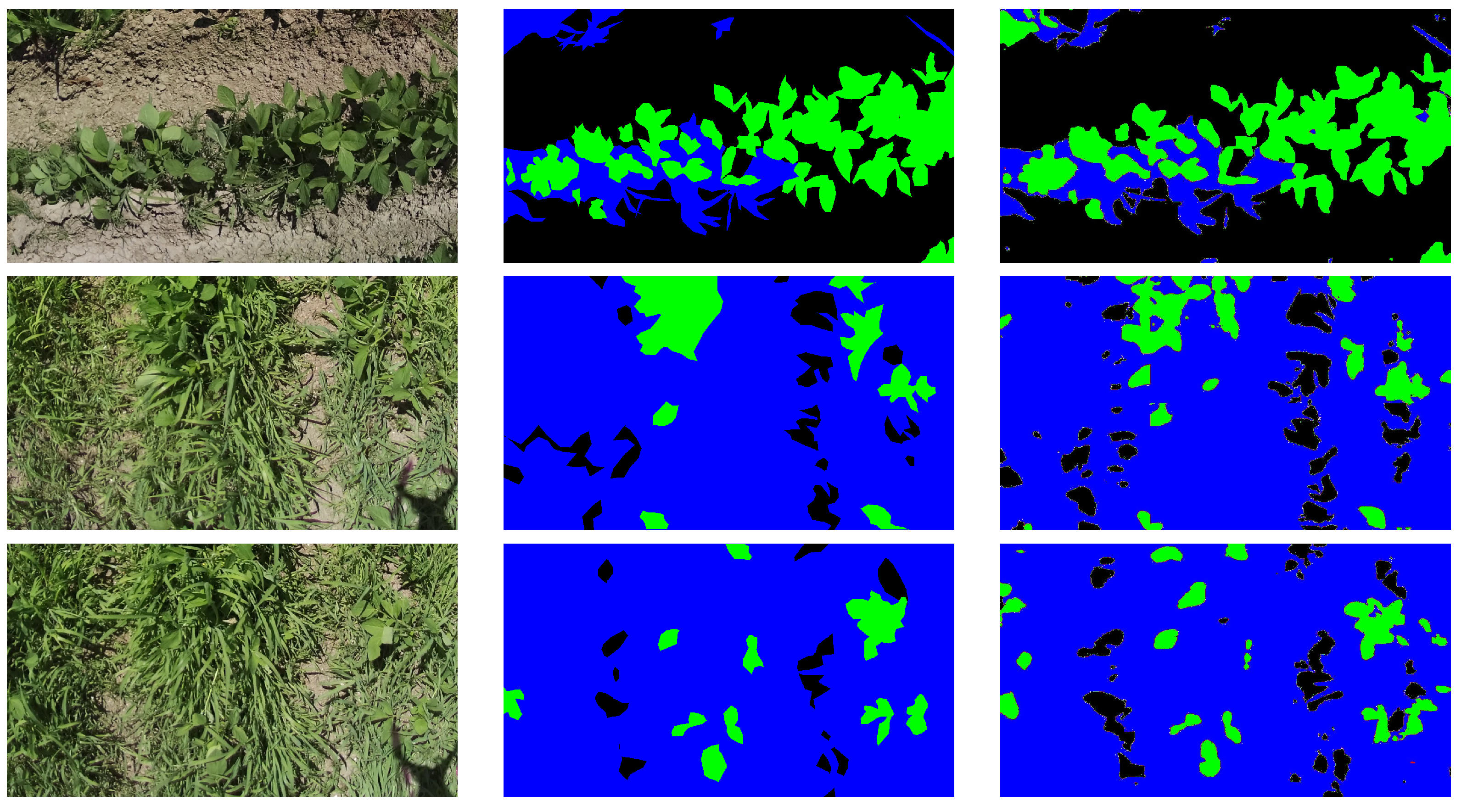
4.1.3. Soybeans
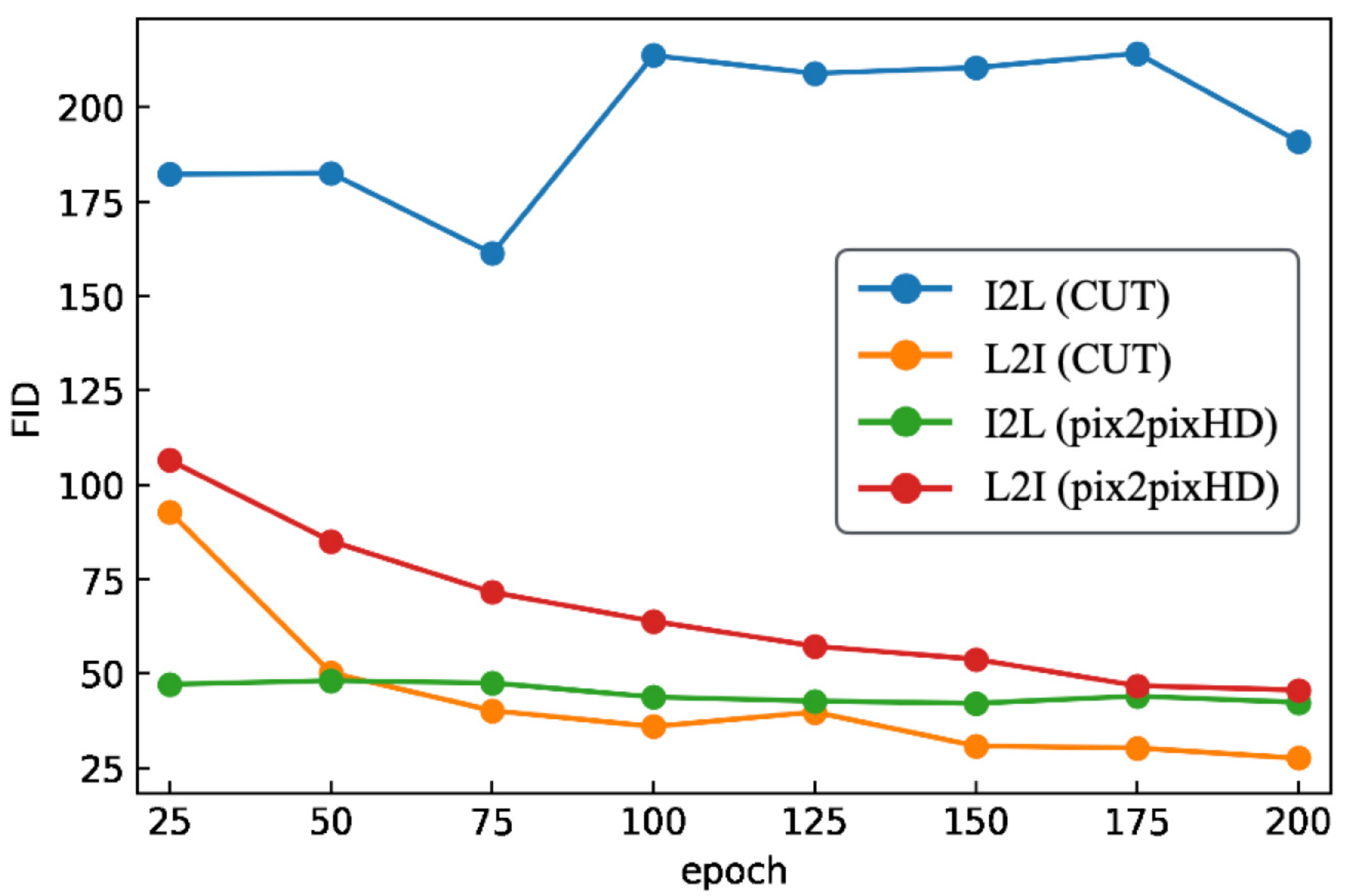
4.2. Evaluation Metrics
5. Preliminary Experiment
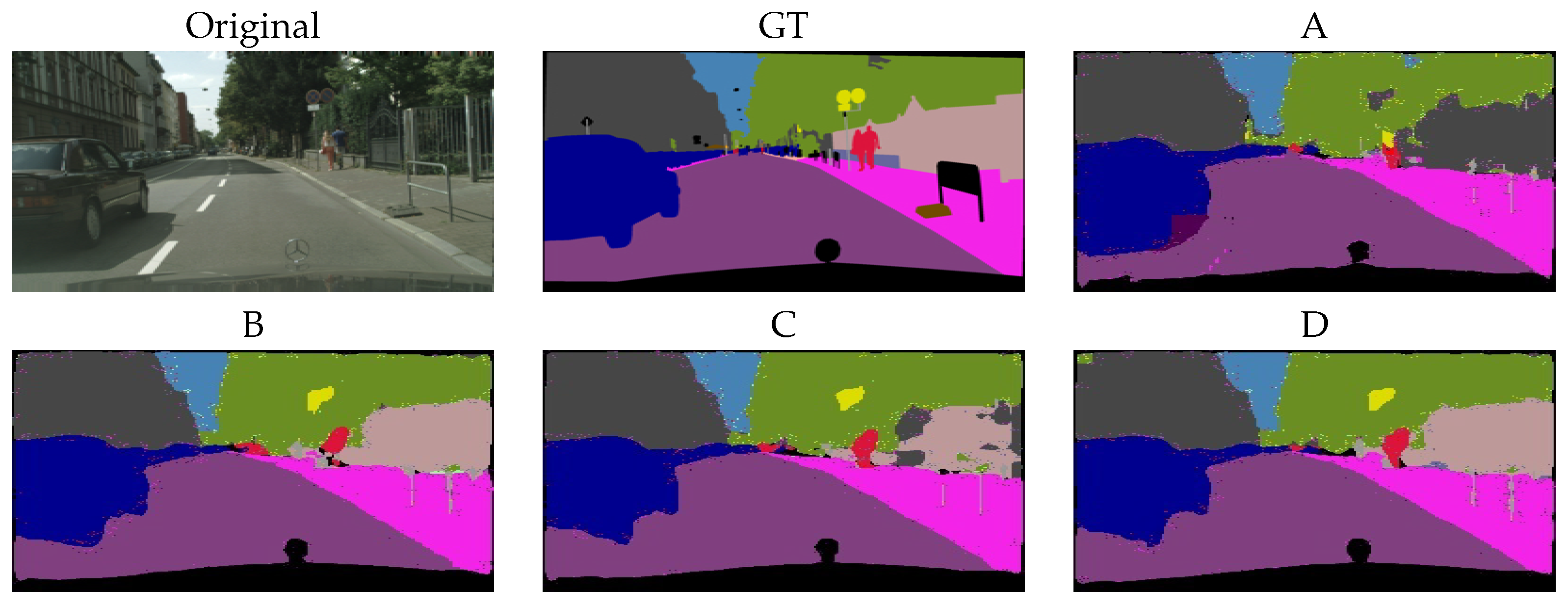
5.1. Cityscapes
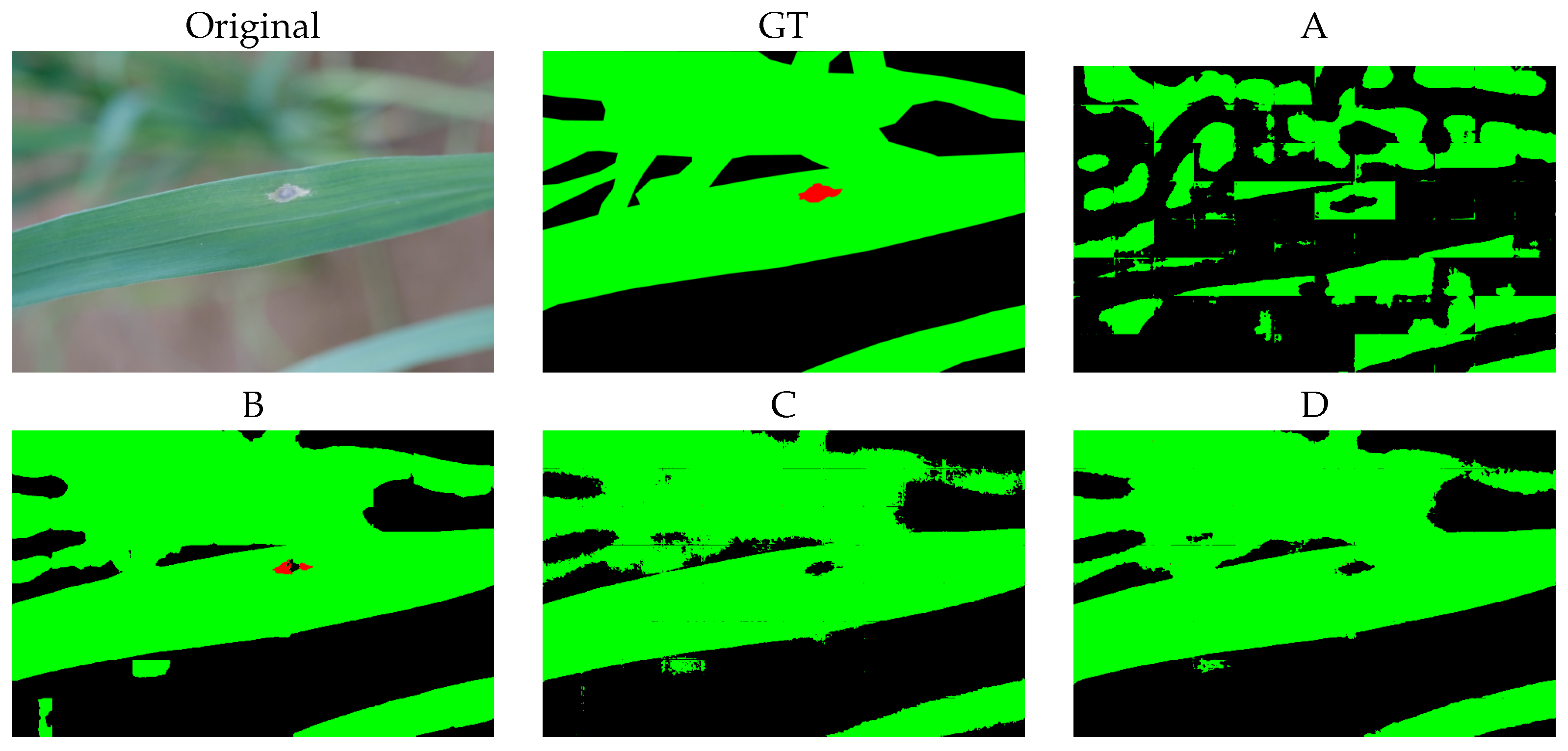
5.2. Rice Blast
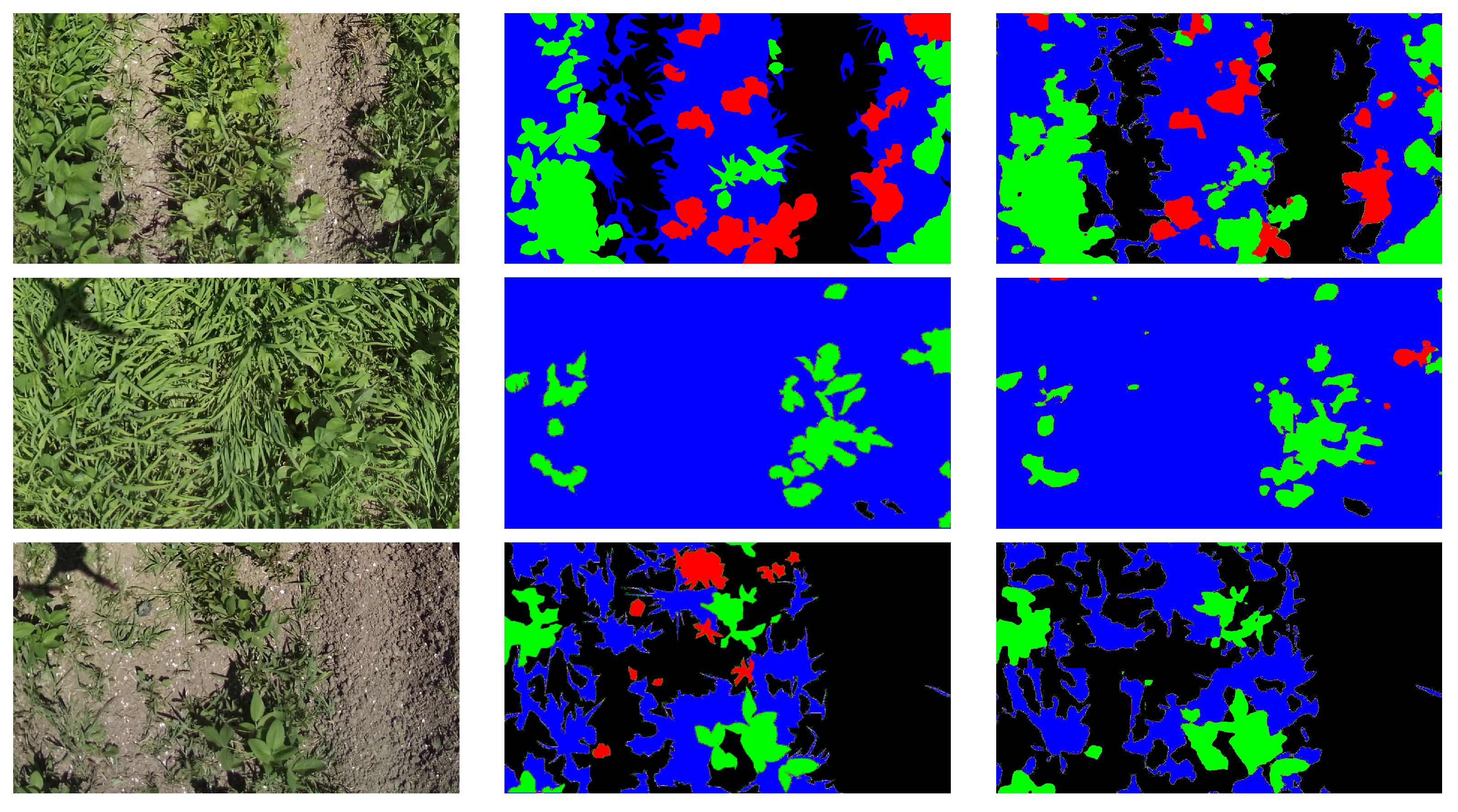
5.3. Soybeans
6. Evaluation Experiment
6.1. Setup
6.2. Baseline
6.2.1. Cityscapes
6.2.2. Rice Blast
6.2.3. Soybeans
6.3. Experiment A
6.4. Experiment B
6.5. Experiment C
6.6. Experiment D
6.7. Overall Comparison and Discussion
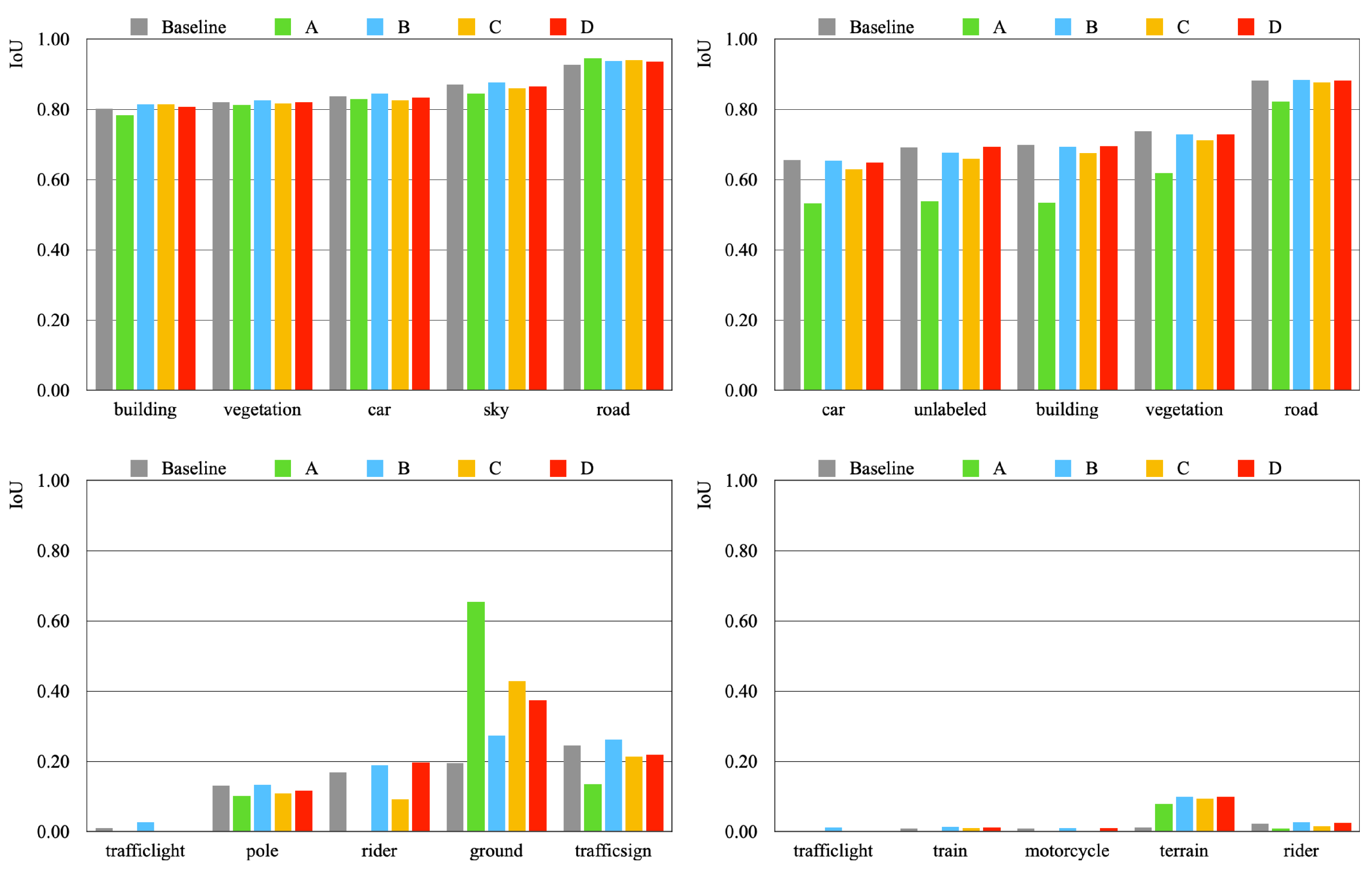
6.7.1. Cityscapes
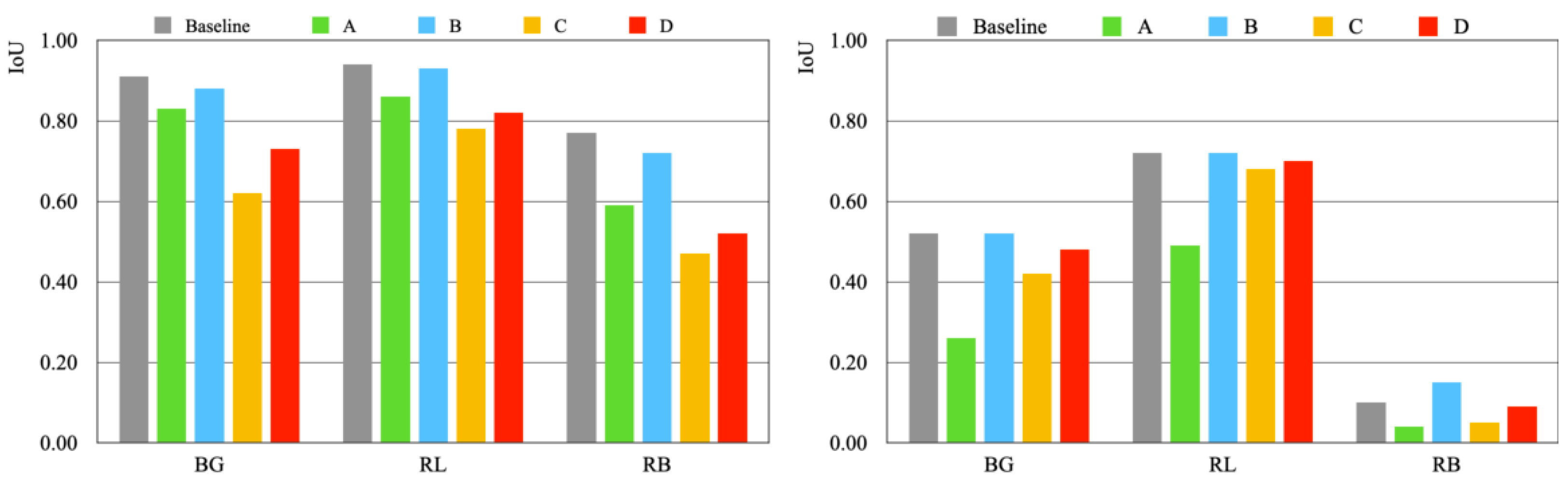
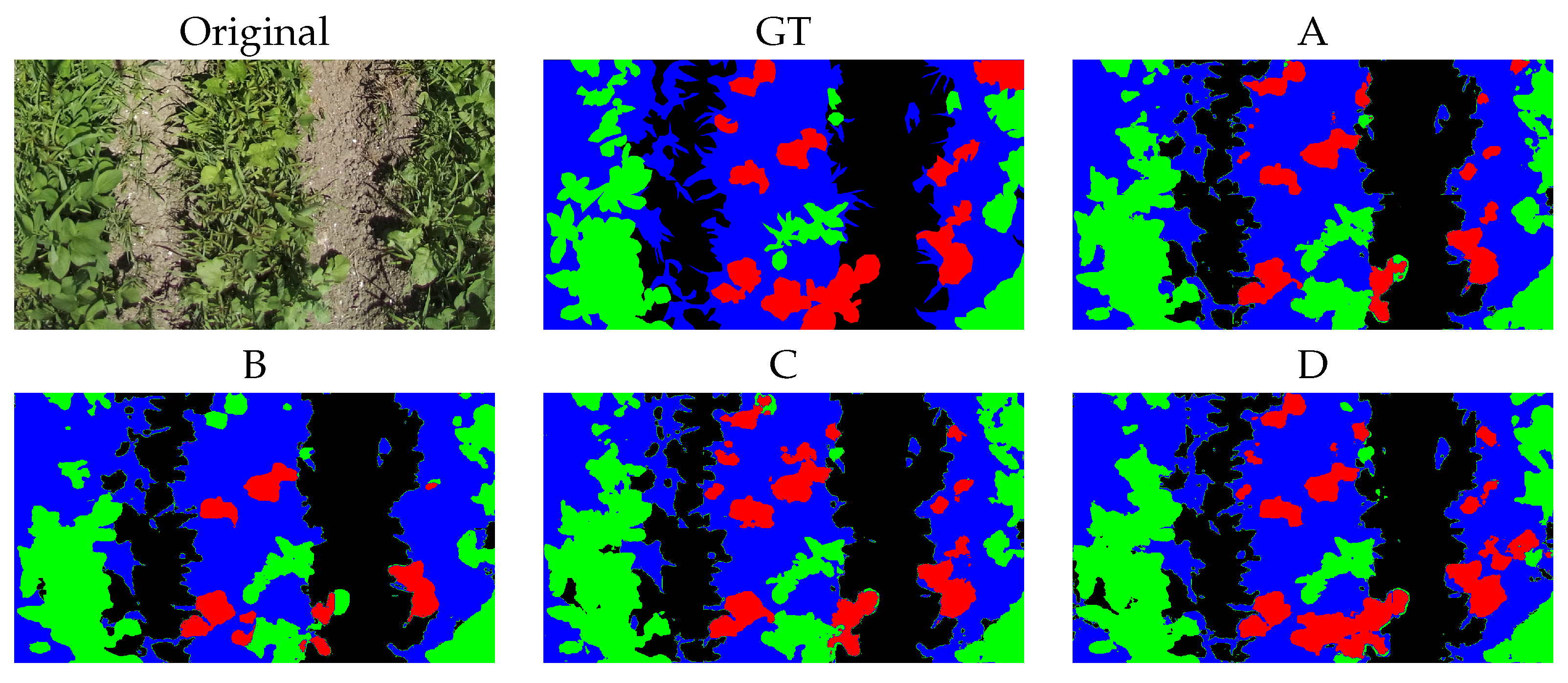
6.7.2. Rice Blast
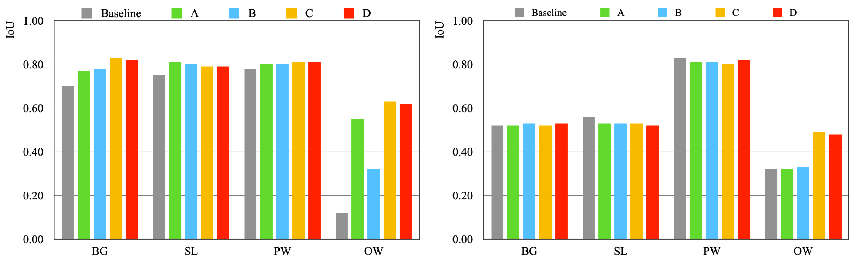
6.7.3. Soybeans
7. Conclusions
Author Contributions
Funding
Institutional Review Board Statement
Informed Consent Statement
Data Availability Statement
Acknowledgments
Conflicts of Interest
Abbreviations
| BG | Background |
| BEGAN | Boundary equilibrium generative adversarial network |
| CAE | Convolutional auto encoder |
| CCL | Cycle consistency loss |
| CL | Contrastive learning |
| CMT | Conventional machine-learning |
| CUT | Contrastive unpaired translation |
| DCGAN | Deep convolutional generative adversarial network |
| DL | Deep learning |
| EBGAN | Energy-based generative adversarial network |
| ESRGAN | Enhanced super-resolution generative adversarial network |
| FID | Fréchet Inception distance |
| GAN | Generative adversarial network |
| GNSS | Global navigation satellite systems |
| GT | Ground truth |
| I2L | Image to label |
| IoT | Internet of things |
| IoU | Intersection over union |
| L2I | Label to image |
| OASIS | Only adversarial supervision for semantic image segmentation |
| OW | Other weeds |
| PGGAN | Progressive growing generative adversarial network |
| PW | Poaceae weeds |
| RB | Rice blast |
| RoI | Region of interest |
| RL | Rice leaves |
| SL | Soybean leaves |
| SPADE | Spatially adaptive denormalization |
| SSL | Self-supervised learning |
| USIS | Unsupervised paradigm for semantic image synthesis |
| ViT | Vision transformer |
References
- Saiz-Rubio, V.; Rovira-Más, F. From Smart Farming towards Agriculture 5.0: A Review on Crop Data Management. Agronomy 2020, 10, 207. [Google Scholar] [CrossRef] [Green Version]
- Farooq, M.S.; Riaz, S.; Abid, A.; Abid, K.; Naeem, M.A. A Survey on the Role of IoT in Agriculture for the Implementation of Smart Farming. IEEE Access 2019, 7, 156237–156271. [Google Scholar] [CrossRef]
- Murugan, D.; Garg, A.; Singh, D. Development of an Adaptive Approach for Precision Agriculture Monitoring with Drone and Satellite Data. IEEE J. Sel. Top. Appl. Earth Obs. Remote Sens. 2017, 10, 12, 5322–5328. [Google Scholar] [CrossRef]
- LeCun, Y.; Bengio, Y.; Hinton, G. Deep learning. Nature 2015, 521, 436–444. [Google Scholar] [CrossRef] [PubMed]
- Kamilaris, A.; Prenafeta-Boldú, F.X. Deep learning in agriculture: A survey. Comput. Electron. Agric. 2018, 147, 70–90. [Google Scholar] [CrossRef] [Green Version]
- Kiran, B.R.; Sobh, I.; Talpaert, V.; Mannion, P.; Sallab, A.A.A.; Yogamani, S.; Pérez, P. Deep Reinforcement Learning for Autonomous Driving: A Survey. IEEE Trans. Intell. Transp. Syst. 2021, 23, 4909–4926. [Google Scholar] [CrossRef]
- Sundararajan, K.; Woodard, D.L. Deep Learning for Biometrics: A Survey. ACM Comput. Surv. 2019, 51, 65. [Google Scholar] [CrossRef]
- Litjens, G.; Kooi, T.; Bejnordi, B.E.; Setio, A.A.A.; Ciompi, F.; Ghafoorian, M.; Laak, J.A.W.M.; Ginneken, B.; Sánchez, C.I. A survey on deep learning in medical image analysis. Med. Image Anal. 2017, 42, 60–88. [Google Scholar] [CrossRef] [Green Version]
- Sharma, A.; Jain, A.; Gupta, P.; Chowdary, V. Machine Learning Applications for Precision Agriculture: A Comprehensive Review. IEEE Access 2021, 9, 4843–4873. [Google Scholar] [CrossRef]
- Liakos, K.G.; Busato, P.; Moshou, D.; Pearson, S.; Bochtis, D. Machine Learning in Agriculture: A Review. Sensors 2018, 18, 2674. [Google Scholar] [CrossRef] [PubMed] [Green Version]
- Benos, L.; Tagarakis, A.C.; Dolias, G.; Berruto, R.; Kateris, D.; Bochtis, D. Machine Learning in Agriculture: A Comprehensive Updated Review. Sensors 2021, 21, 3758. [Google Scholar] [CrossRef] [PubMed]
- Balducci, F.; Impedovo, D.; Pirlo, G. Machine Learning Applications on Agricultural Datasets for Smart Farm Enhancement. Machines 2018, 6, 38. [Google Scholar] [CrossRef] [Green Version]
- Wolfert, S.; Ge, L.; Verdouw, C.; Bogaardt, M.-J. Big Data in Smart Farming: A review. Agric. Syst. 2017, 153, 69–80. [Google Scholar] [CrossRef]
- Lu, X.; Wang, W.; Shen, J.; Tai, Y.-W.; Crandall, D.J.; Hoi, S.C.H. Learning Video Object Segmentation From Unlabeled Videos. In Proceedings of the IEEE Conference on Computer Vision and Pattern Recognition (CVPR), Virtual, 14–19 June 2020; pp. 8960–8970. [Google Scholar]
- Du, X.; Jiang, C.; Xu, H.; Zhang, G.; Li, Z. How to Save your Annotation Cost for Panoptic Segmentation? In Proceedings of the AAAI Conference on Artificial Intelligence, Virtual, 2–9 February 2021; pp. 1282–1290. [Google Scholar]
- Unal, Z. Smart Farming Becomes Even Smart with Deep Learning—A Bibliographical Analysis. IEEE Access 2020, 8, 105587–105609. [Google Scholar] [CrossRef]
- Thoma, M. A survey of semantic segmentation. arXiv 2016, arXiv:1602.06541. [Google Scholar]
- Milioto, A.; Lottes, P.; Stachniss, C. Real-Time Semantic Segmentation of Crop and Weed for Precision Agriculture Robots Leveraging Background Knowledge in CNNs. In Proceedings of the IEEE International Conference on Robotics and Automation (ICRA), Brisbane, QLD, Australia, 21–25 May 2018; pp. 2229–2235. [Google Scholar]
- Kirillov, A.; He, K.; Girshick, R.; Rother, C.; Dollar, P. Panoptic Segmentation. In Proceedings of the IEEE Conference on Computer Vision and Pattern Recognition (CVPR), Long Beach, CA, USA, 16–20 June 2019; pp. 9404–9413. [Google Scholar]
- Champ, J.; Mora-Fallas, A.; Goëau, H.; Mata-Montero, E.; Bonnet, P.; Joly, A. Instance segmentation for the fine detection of crop and weed plants by precision agricultural robots. Appl. Plant Sci. 2020, 8, e11373. [Google Scholar] [CrossRef] [PubMed]
- He, K.; Gkioxari, G.; Dollár, P.; Girshick, R. MaskR-CNN. In Proceedings of the IEEE International Conference on Computer Vision, (ICCV), Venice, Italy, 22–29 October 2017; pp. 2961–2969. [Google Scholar]
- Zheng, Y.-Y.; Kong, J.-L.; Jin, X.-B.; Wang, X.-Y.; Su, T.-L.; Zuo, M. CropDeep: The Crop Vision Dataset for Deep-Learning-Based Classification and Detection in Precision Agriculture. Sensors 2019, 19, 1058. [Google Scholar] [CrossRef] [PubMed] [Green Version]
- Singh, A.; Jaiswal, V.; Joshi, G.; Sanjeeve, A.; Gite, S.; Kotecha, K. Neural Style Transfer: A Critical Review. IEEE Access 2021, 9, 131583–131613. [Google Scholar] [CrossRef]
- Gatys, L.A.; Ecker, A.S.; Bethge, M. Image Style Transfer Using Convolutional Neural Networks. In Proceedings of the IEEE Conference on Computer Vision and Pattern Recognition (CVPR), Las Vegas, NV, USA, 26 June–1 July 2016; pp. 2414–2423. [Google Scholar]
- Goodfellow, I.; Pouget-Abadie, J.; Mirza, M.; Xu, B.; Warde-Farley, D.; Ozair, S.; Courville, A.; Bengio, Y. Generative Adversarial Networks. In Proceedings of the International Conference on Neural Information Processing Systems (NIPS), Montreal, QC, Canada, 8–13 December 2014; pp. 2672–2680. [Google Scholar]
- Rozantsev, A.; Lepetit, V.; Fua, P. On rendering synthetic images for training an object detector. arXiv 2014, arXiv:1411.7911. [Google Scholar] [CrossRef] [Green Version]
- Rematas, K.; Ritschel, T.; Fritz, M.; Tuytelaars, T. Image-based Synthesis and Re-Synthesis of Viewpoints Guided by 3D Models. In Proceedings of the IEEE Conference on Computer Vision and Pattern Recognition (CVPR), Columbus, OH, USA, 24–27 June 2014; pp. 3898–3905. [Google Scholar]
- Pishchulin, L.; Jain, A.; Andriluka, M. Articulated People Detection and Pose Estimation: Reshaping the Future. In Proceedings of the IEEE Conference on Computer Vision and Pattern Recognition (CVPR), Providence, RI, USA, 16–21 June 2012; pp. 3178–3185. [Google Scholar]
- Vázquez, D.; López, A.M.; Marin, J.; Ponsa, D.; Gerónimo, D. Virtual and real world adaptation for pedestrian detection. IEEE Trans. Pattern Anal. Mach. Intell. 2014, 36, 4, 797–809. [Google Scholar] [CrossRef]
- Ros, G.; Sellart, L.; Materzynska, J.; Vazquez, D.; Lopez, A.M. The SYNTHIA Dataset: A Large Collection of Synthetic Images for Semantic Segmentation of Urban Scenes. In Proceedings of the IEEE Conference on Computer Vision and Pattern Recognition (CVPR), Las Vegas, NV, USA, 26 June–1 July 2016; pp. 3234–3243. [Google Scholar]
- LeCun, Y.; Boser, B.; Denker, J.S.; Henderson, D.; Howard, R.E.; Hubbard, W.; Jackel, L.D. Backpropagation Applied to Handwritten Zip Code Recognition. Neural Comput. 1989, 1, 541–551. [Google Scholar] [CrossRef]
- Simonyan, K.; Zisserman, A. Two-stream convolutional networks for action recognition in videos. In Proceedings of the International Conference on Neural Information Processing Systems (NIPS), Montreal, QC, Canada, 8–13 December 2014. [Google Scholar]
- Szegedy, C.; Vanhoucke, V.; Ioffe, S.; Shlens, J.; Wojna, Z. Rethinking the inception architecture for computer vision. In Proceedings of the IEEE Conference on Computer Vision and Pattern Recognition (CVPR), Las Vegas, NV, USA, 26 June–1 July 2016; pp. 2818–2826. [Google Scholar]
- He, K.; Zhang, X.; Ren, S.; Sun, J. Deep Residual Learning for Image Recognition. In Proceedings of the IEEE Conference on Computer Vision and Pattern Recognition (CVPR), Las Vegas, NV, USA, 26 June–1 July 2016; pp. 770–778. [Google Scholar]
- Xie, S.; Girshick, R.; Dollár, P.; Tu, Z.; He, K. Aggregated residual transformations for deep neural networks. In Proceedings of the IEEE Conference on Computer Vision and Pattern Recognition (CVPR), Honolulu, HI, USA, 21–26 July 2017. [Google Scholar]
- Huang, G.; Liu, Z.; Maaten, L.; Weinberger, K. Densely connected convolutional networks. In Proceedings of the IEEE Conference on Computer Vision and Pattern Recognition (CVPR), Honolulu, HI, USA, 21–26 July 2017. [Google Scholar]
- Howard, A.; Zhu, M.; Chen, B.; Kalenichenko, D.; Wang, W.; Weyand, T.; Andreetto, M.; Adam, H. MobileNets: Efficient convolutional neural networks for mobile vision applications. arXiv 2017, arXiv:1704.04861. [Google Scholar]
- Tan, M.; Le, Q. Efficientnet: Rethinking model scaling for convolutional neural networks. In Proceedings of the 36th International Conference on Machine Learning (ICML), Long Beach, CA, USA, 9–15 June 2019. [Google Scholar]
- Radosavovic, I.; Kosaraju, R.P.; Girshick, R.; He, K.; Dollár, P. Designing network design spaces. In Proceedings of the IEEE Conference on Computer Vision and Pattern Recognition (CVPR), Virtual, 14–19 June 2020; pp. 5549–5558. [Google Scholar]
- Vaswani, A.; Shazeer, N.; Parmar, N.; Uszkoreit, J.; Jones, L.; Gomez, A.N.; Kaiser, L.; Polosukhin, I. Attention is All You Need. In Proceedings of the Conference on Neural Information Processing Systems (NIPS), Long Beach, CA, USA, 4–9 December 2017. [Google Scholar]
- Xie, E.; Wang, W.; Yu, Z.; Anandkumar, A.; Alvarez, J.M.; Luo, P. SegFormer: Simple and Efficient Design for Semantic Segmentation with Transformers. In Proceedings of the Conference on Neural Information Processing Systems (NIPS), Virtual, 6–14 December 2021. [Google Scholar]
- Strudel, R.; Garcia, R.; Laptev, I.; Schmid, C. Segmenter: Transformer for Semantic Segmentation. In Proceedings of the International Conference on Computer Vision (ICCV), Virtual, 11–17 October 2021; pp. 7262–7272. [Google Scholar]
- Zheng, S.; Lu, J.; Zhao, H.; Zhu, X.; Luo, Z.; Wang, Y.; Fu, Y.; Feng, J.; Xiang, T.; Torr, Z.P.H.S.; et al. Rethinking Semantic Segmentation From a Sequence-to-Sequence Perspective With Transformers. In Proceedings of the IEEE Conference on Computer Vision and Pattern Recognition (CVPR), Virtual, 19–25 June 2021; pp. 6881–6890. [Google Scholar]
- Liu, Z.; Lin, Y.; Cao, Y.; Hu, H.; Wei, Y.; Zhang, Z.; Lin, S.; Guo, B. Swin Transformer: Hierarchical Vision Transformer Using Shifted Windows. In Proceedings of the International Conference on Computer Vision (ICCV), Virtual, 11–17 October 2021; pp. 10012–10022. [Google Scholar]
- Tran, N.-T.; Tran, V.-H.; Nguyen, N.-B.; Nguyen, T.-K.; Cheung, N.-M. On Data Augmentation for GAN Training. IEEE Trans. Image Process. 2021, 30, 1882–1897. [Google Scholar] [CrossRef]
- Tanaka, F.H.K.S.; Aranha, C. Data Augmentation Using GANs. arXiv 2019, arXiv:1904.09135. [Google Scholar]
- Shorten, C.; Khoshgoftaar, T.M. A survey on Image Data Augmentation for Deep Learning. J. Big Data 2019, 6, 60. [Google Scholar] [CrossRef]
- Huang, S.-W.; Lin, C.-T.; Chen, S.-P.; Wu, Y.-Y.; Hsu, P.-H.; Lai, S.-H. AugGAN: Cross Domain Adaptation with GAN-based Data Augmentation. In Proceedings of the European Conference on Computer Vision (ECCV), Munich, Germany, 8–14 September 2018; pp. 718–731. [Google Scholar]
- Choi, J.; Kim, T.; Kim, C. Self-Ensembling with GAN-Based Data Augmentation for Domain Adaptation in Semantic Segmentation. In Proceedings of the International Conference on Computer Vision (ICCV), Seoul, Korea, 27 October–2 November 2017; pp. 6830–6840. [Google Scholar]
- Vilkas, E. Axiomatic definition of the value of a matrix game. Theory Probab. Appl. 1963, 8, 304–307. [Google Scholar] [CrossRef]
- Radford, A.; Metz, L. Unsupervised Representation Learning with Deep Convolutional Generative Adversarial Networks. arXiv 2015, arXiv:1511.06434. [Google Scholar]
- Zhao, J.; Mathieu, M.; LeCun, Y. Energy-based Generative Adversarial Network. arXiv 2017, arXiv:1609.03126. [Google Scholar]
- Berthelot, D.; Schumm, T.; Metz, L. BEGAN: Boundary Equilibrium Generative Adversarial Networks. arXiv 2017, arXiv:1703.10717. [Google Scholar]
- Hinton, G.E.; Salakhutdinov, R.R. Reducing the Dimensionality of Data with Neural Networks. Science 2006, 313, 504–507. [Google Scholar] [CrossRef] [PubMed] [Green Version]
- Karras, T.; Aila, T.; Laine, S.; Lehtinen, J. Progressive Growing of GAN for Improved Quality, Stability, and Variation. arXiv 2018, arXiv:1710.10196. [Google Scholar]
- Huang, X.; Belongie, S.J. Arbitrary style transfer in real-time with adaptive instance normalization. arXiv 2017, arXiv:1703.06868. [Google Scholar]
- Karras, T.; Laine, S.; Aila, T. A Style-Based Generator Architecture for Generative Adversarial Networks. In Proceedings of the IEEE Conference on Computer Vision and Pattern Recognition (CVPR), Long Beach, CA, USA, 16–20 June 2019; pp. 4401–4410. [Google Scholar]
- Bermano, A.H.; Gal, R.; Alaluf, Y.; Mokady, R.; Nitzan, Y.; Tov, O.; Patashnik, O.; Cohen-Or, D. State-of-the-Art in the Architecture, Methods and Applications of StyleGAN. arXiv 2022, arXiv:2202.14020. [Google Scholar] [CrossRef]
- Wang, X.; Yu, K.; Wu, S.; Gu, J.; Liu, Y.; Dong, C.; Loy, C.C.; Qiao, Y.; Tang, X. ESRGAN: Enhanced Super-Resolution Generative Adversarial Networks. In Proceedings of the European Conference on Computer Vision (ECCV), Munich, Germany, 8–14 September 2018. [Google Scholar]
- Zhang, H.; Xu, T.; Li, H.; Zhang, S.; Wang, X.; Huang, X.; Metaxas, D. StackGAN: Text to Photo-realistic Image Synthesis with Stacked Generative Adversarial Networks. In Proceedings of the International Conference on Computer Vision (ICCV), Venice, Italy, 22–29 October 2017; pp. 5907–5915. [Google Scholar]
- Jing, Y.; Yang, Y.; Feng, Z.; Ye, J.; Yu, Y.; Song, M. Neural Style Transfer: A Review. IEEE Trans. Vis. Comput. Graph. 2020, 26, 3365–3385. [Google Scholar] [CrossRef] [PubMed] [Green Version]
- Zhao, W.; Yamada, W.; Li, T.; Digman, M.; Runge, T. Augmenting Crop Detection for Precision Agriculture with Deep Visual Transfer Learning—Case Study of Bale Detection. Remote Sens. 2021, 13, 23. [Google Scholar] [CrossRef]
- Mirza, M.; Osindero, S. Conditional Generative Adversarial Nets. arXiv 2014, arXiv:1411.1784. [Google Scholar]
- Isola, P.; Zhu, J.Y.; Zhou, T.; Efros, A.A. Image-to-image translation with conditional adversarial networks. In Proceedings of the IEEE Conference on Computer Vision and Pattern Recognition (CVPR), Honolulu, HI, USA, 21–26 July 2017; pp. 1125–1134. [Google Scholar]
- Wang, T.C.; Liu, M.Y.; Tao, A.; Kautz, J.; Catanzaro, B. High-Resolution Image Synthesis and Semantic Manipulation with Conditional GAN. In Proceedings of the IEEE Conference on Computer Vision and Pattern Recognition (CVPR), Salt Lake City, UT, USA, 19–21 June 2018; pp. 8798–8807. [Google Scholar]
- Lee, C.H.; Liu, Z.; Wu, L.; Luo, P. Maskgan: Towards diverse and interactive facial image manipulation. In Proceedings of the IEEE Conference on Computer Vision and Pattern Recognition (CVPR), Virtual, 14–19 June 2020; pp. 5549–5558. [Google Scholar]
- Park, T.; Liu, M.Y.; Wang, T.C.; Zhu, J.Y. Semantic image synthesis with spatially adaptive normalization. In Proceedings of the IEEE Conference on Computer Vision and Pattern Recognition (CVPR), Long Beach, CA, USA, 16–20 June 2019; pp. 4401–4410. [Google Scholar]
- Sushko, V.; Schonfeld, E.; Zhang, D.; Gall, J.; Schiele, B.; Khoreva, A. You Only Need Adversarial Supervision for Semantic Image Synthesis. In Proceedings of the International Conference on Learning Representations (ICLR), Virtual, 3–7 May 2021. [Google Scholar]
- Simonyan, K.; Zisserman, A. Very Deep Convolutional Networks for Large-Scale Image Recognition. arXiv 2015, arXiv:1409.1556. [Google Scholar]
- Zhu, J.Y.; Park, T.; Isola, P.; Efros, A.A. Unpaired image-to-image translation using cycle-consistent adversarial networks. In Proceedings of the International Conference on Computer Vision (ICCV), Venice, Italy, 22–29 October 2017; pp. 2223–2232. [Google Scholar]
- Park, T.; Efros, A.A.; Zhang, R.; Zhu, J.Y. Contrastive Learning for Unpaired Image-to-Image Translation. In Proceedings of the European Conference on Computer Vision (ECCV), Virtual, 23–28 August 2020; pp. 319–345. [Google Scholar]
- Ronneberger, O.; Fischer, P.; Brox, T. U-Net: Convolutional Networks for Biomedical Image Segmentation. In Proceedings of the Medical Image Computing and Computer-Assisted Intervention (MICCAI), Munich, Germany, 5–9 October 2015; pp. 234–241. [Google Scholar]
- Eskandar, G.; Abdelsamad, M.; Armanious, K.; Yang, B. USIS: Unsupervised Semantic Image Synthesis. arXiv 2021, arXiv:2109.14715. [Google Scholar]
- Jaiswal, A.; Babu, A.R.; Zadeh, M.Z.; Banerjee, D.; Makedon, F.A. Survey on Contrastive Self-Supervised Learning. Technologies 2021, 9, 2. [Google Scholar] [CrossRef]
- Eskandar, G.; Abdelsamad, M.; Armanious, K.; Zhang, S.; Yang, B. Wavelet-Based Unsupervised Label-to-Image Translation. In Proceedings of the IEEE International Conference on Acoustics, Speech and Signal Processing (ICASSP), Singapore, 23–27 May 2022; pp. 1760–1764. [Google Scholar]
- Cao, Y.-J.; Jia, L.-L.; Chen, Y.-X.; Lin, N.; Yang, C.; Zhang, B.; Liu, Z.; Li, X.-X.; Dai, H.-H. Recent Advances of Generative Adversarial Networks in Computer Vision. IEEE Access 2018, 7, 14985–15006. [Google Scholar] [CrossRef]
- Pan, Z.; Yu, W.; Yi, X.; Khan, A.; Yuan, F.; Zheng, Y. Recent Progress on Generative Adversarial Networks (GANs): A Survey. IEEE Access 2019, 7, 36322–36333. [Google Scholar] [CrossRef]
- Hajarolasvadi, N.; Ramírez, M.A.; Beccaro, W.; Demirel, H. Generative Adversarial Networks in Human Emotion Synthesis: A Review. IEEE Access 2020, 8, 218499–218529. [Google Scholar] [CrossRef]
- Dekker, J. Weed diversity and weed management. Weed Sci. 1997, 45, 357–363. [Google Scholar] [CrossRef]
- Madokoro, H.; Yamamoto, S.; Nishimura, Y.; Nix, S.; Woo, H.; Sato, K. Prototype Development of Small Mobile Robots for Mallard Navigation in Paddy Fields: Toward Realizing Remote Farming. Robotics 2021, 10, 63. [Google Scholar] [CrossRef]
- Minaee, S.; Boykov, Y.Y.; Porikli, F.; Plaza, A.J.; Kehtarnavaz, N.; Terzopoulos, D. Image Segmentation Using Deep Learning: A Survey. IEEE Trans. Pattern Anal. Mach. Intell. 2021, 44, 3523–3542. [Google Scholar] [CrossRef]
- Liu, X.; Deng, Z.; Yang, Y. Recent progress in semantic image segmentation. Artif. Intell. Rev. 2019, 52, 1089–1106. [Google Scholar] [CrossRef] [Green Version]
- Yu, H.; Yang, Z.; Tan, L.; Wang, Y.; Sun, W.; Sun, M.; Tang, Y. Methods and datasets on semantic segmentation: A review. Neurocomputing 2018, 304, 82–103. [Google Scholar] [CrossRef]
- Fahim, M.A.-N.I.; Jung, H.Y. A Lightweight GAN Network for Large Scale Fingerprint Generation. IEEE Access 2020, 8, 92918–92928. [Google Scholar] [CrossRef]
- Chen, T.; Kornblith, S.; Norouzi, M.; Hinton, G. A simple framework for contrastive learning of visual representations. In Proceedings of the 36th International Conference on Machine Learning (ICML), Virtual, 13–18 July 2020; pp. 1597–1607. [Google Scholar]
- Pang, T.; Xu, K.; Dong, Y.; Du, C.; Chen, N.; Zhu, J. Rethinking Softmax Cross-Entropy Loss for Adversarial Robustness. arXiv 2020, arXiv:1905.10626. [Google Scholar]
- Krause, E.F. Taxicab Geometry. Math. Teach. 1973, 66, 8, 695–706. [Google Scholar] [CrossRef]
- Toldo, M.; Maracani, A.; Michieli, U.; Zanuttigh, P. Unsupervised Domain Adaptation in Semantic Segmentation: A Review. Technologies 2020, 8, 35. [Google Scholar] [CrossRef]
- Zhang, S.; Benenson, R.; Schiele, B. CityPersons: A Diverse Dataset for Pedestrian Detection. In Proceedings of the IEEE Conference on Computer Vision and Pattern Recognition (CVPR), Honolulu, HI, USA, 21–26 July 2017; pp. 3213–3221. [Google Scholar]
- Huang, M.L.; Wu, Y.Z. Semantic segmentation of pancreatic medical images by using convolutional neural network. Biomed. Signal Process. Control 2022, 73, 1746–8094. [Google Scholar] [CrossRef]
- Ivanovs, M.; Ozols, K.; Dobrajs, A.; Kadikis, R. Improving Semantic Segmentation of Urban Scenes for Self-Driving Cars with Synthetic Images. Sensors 2022, 22, 2252. [Google Scholar] [CrossRef] [PubMed]
- Kerle, N.; Nex, F.; Gerke, M.; Duarte, D.; Vetrivel, A. UAV-Based Structural Damage Mapping: A Review. ISPRS Int. J. Geo-Inf. 2020, 9, 14. [Google Scholar] [CrossRef] [Green Version]
- Yu, R.; Li, H.; Jiang, Y.; Zhang, B.; Wang, Y. Tiny Vehicle Detection for Mid-to-High Altitude UAV Images Based on Visual Attention and Spatial–Temporal Information. Sensors 2022, 22, 2354. [Google Scholar] [CrossRef]
- Xu, Z.; Zhang, W.; Zhang, T.; Li, J. HRCNet: High-Resolution Context Extraction Network for Semantic Segmentation of Remote Sensing Images. Remote Sens. 2021, 13, 71. [Google Scholar] [CrossRef]
- Costa, M.V.C.V.d.; Carvalho, O.L.F.d.; Orlandi, A.G.; Hirata, I.; Albuquerque, A.O.d.; Silva, F.V.e.; Guimarães, R.F.; Gomes, R.A.T.; Júnior, O.A.d.C. Remote Sensing for Monitoring Photovoltaic Solar Plants in Brazil Using Deep Semantic Segmentation. Energies 2021, 14, 2960. [Google Scholar] [CrossRef]
- Yang, L.; Fan, J.; Liu, Y.; Li, E.; Peng, J.; Liang, Z. A Review on State-of-the-Art Power Line Inspection Techniques. IEEE Trans. Instrum. Meas. 2020, 69, 9350–9365. [Google Scholar] [CrossRef]
- Shin, Y.-H.; Son, K.-W.; Lee, D.-C. Semantic Segmentation and Building Extraction from Airborne LiDAR Data with Multiple Return Using PointNet++. Appl. Sci. 2022, 12, 1975. [Google Scholar] [CrossRef]
- Craye, C.; Ardjoune, S. Spatiotemporal Semantic Segmentation for Drone Detection. In Proceedings of the 16th IEEE International Conference on Advanced Video and Signal Based Surveillance (AVSS), Taipei, Taiwan, 18–21 September 2019; pp. 1–5. [Google Scholar]
- Ramirez-Amaro, K.; Minhas, H.N.; Zehetleitner, M.; Beetz, M.; Cheng, G. Added value of gaze-exploiting semantic representation to allow robots inferring human behaviors. ACM Trans. Interact. Intell. Syst. 2017, 7, 1–30. [Google Scholar] [CrossRef]
- Lundgren, A.V.A.; Santos, M.A.O.d.; Bezerra, B.L.D.; Bastos-Filho, C.J.A. Systematic Review of Computer Vision Semantic Analysis in Socially Assistive Robotics. AI 2022, 3, 229–249. [Google Scholar] [CrossRef]
- Xu, H.; Chen, G.; Wang, Z.; Sun, L.; Su, F. RGB-D-Based Pose Estimation of Workpieces with Semantic Segmentation and Point Cloud Registration. Sensors 2019, 19, 1873. [Google Scholar] [CrossRef] [PubMed] [Green Version]
- Badrinarayanan, V.; Kendall, A.; Cipolla, R. Segnet: A deep convolutional encoder-decoder architecture for image segmentation. IEEE Trans. Pattern Anal. Mach. Intell. 2017, 39, 2481–2495. [Google Scholar] [CrossRef] [PubMed]
- Chen, L.C.; Zhu, Y.; Papandreou, G.; Schroff, F.; Adam, H. Encoder–Decoder with Atrous Separable Convolution for Semantic Image Segmentation. In Proceedings of the European Conference on Computer Vision (ECCV), Munich, Germany, 8–14 September 2018; pp. 801–818. [Google Scholar]
- Sun, K.; Zhao, Y.; Jiang, B.; Cheng, T.; Xiao, B.; Liu, D.; Mu, Y.; Wang, X.; Liu, W.; Wang, J. High-Resolution Representations for Labeling Pixels and Regions. arXiv 2019, arXiv:1904.04514. [Google Scholar]
- Liu, Z.; Mao, H.; Wu, C.-Y.; Feichtenhofer, C.; Darrell, T.; Xie, S. A ConvNet for the 2020s. In Proceedings of the IEEE Conference on Computer Vision and Pattern Recognition (CVPR), New Orleans, LA, USA, 19–24 June 2022; pp. 11976–11986. [Google Scholar]
- Dosovitskiy, A.; Beyer, L.; Kolesnikov, A.; Weissenborn, D.; Zhai, X.; Unterthiner, T.; Dehghani, M.; Minderer, M.; Heigold, G.; Gelly, S.; et al. An image is worth 16x16 words: Transformers for image recognition at scale. arXiv 2020, arXiv:2010.11929. [Google Scholar]
- Tuli, S.; Dasgupta, I.; Grant, E.; Griffiths, T.L. Are Convolutional Neural Networks or Transformers more like human vision? arXiv 2021, arXiv:2105.07197. [Google Scholar]
- Raghu, M.; Unterthiner, T.; Kornblith, S.; Zhang, C.; Dosovitskiy, A. Do Vision Transformers See Like Convolutional Neural Networks? In Proceedings of the Conference on Neural Information Processing Systems (NIPS), Virtual, 6–14 December 2021. [Google Scholar]
- Steiner, A.; Kolesnikov, A.; Zhai, X.; Wightman, R.; Uszkoreit, J.; Beyer, L. How to train your ViT? Data, Augmentation, and Regularization in Vision Transformers. arXiv 2021, arXiv:2106.10270. [Google Scholar]
- Ridnik, T.; Ben-Baruch, E.; Noy, A.; Lihi Zelnik-Manor, L. ImageNet-21K Pretraining for the Masses. arXiv 2021, arXiv:2104.10972. [Google Scholar]
- Sun, C.; Shrivastava, A.; Singh, S.; Gupta, A. Revisiting unreasonable effectiveness of data in deep learning era. In Proceedings of the International Conference on Computer Vision (ICCV), Venice, Italy, 22–29 October 2017; pp. 843–852. [Google Scholar]
- Kolesnikov, A.; Beyer, L.; Zhai, X.; Puigcerver, J.; Yung, J.; Gelly, S.; Houlsby, N. Big Transfer (BiT): General Visual Representation Learning. In Proceedings of the European Conference on Computer Vision (ECCV), Virtual, 23–28 August 2020; pp. 491–507. [Google Scholar]
- Caesar, H.; Uijlings, J.; Ferrari, V. COCO-Stuff: Thing and stuff Classes in Context. In Proceedings of the IEEE Conference on Computer Vision and Pattern Recognition (CVPR), Salt Lake City, UT, USA, 19–21 June 2018; pp. 1209–1218. [Google Scholar]
- Sato, K.H.; Madokoro, H.; Nagayoshi, T.; Chiyonobu, S.; Martizzi, P.; Nix, S.; Woo, H.; Saito, T.K.; Sato, K. Semantic Segmentation of Outcrop Images using Deep Learning Networks Toward Realization of Carbon Capture and Storage. In Proceedings of the 17th International Conference on Control, Automation and Systems (ICCAS), Jeju, Korea, 12–15 October 2021; pp. 436–441. [Google Scholar]
- Takahashi, K.H.; Madokoro, H.; Yamamoto, S.; Nishimura, Y.; Nix, S.; Woo, H.; Saito, T.K.; Sato, K. Domain Adaptation for Agricultural Image Recognition and Segmentation Using Category Maps. In Proceedings of the 17th International Conference on Control, Automation and Systems (ICCAS), Jeju, Korea, 12–15 October 2021; pp. 1680–1685. [Google Scholar]
- Chollet, F. Xception: Deep Learning with Depthwise Separable Convolutions. In Proceedings of the IEEE Conference on Computer Vision and Pattern Recognition (CVPR), Honolulu, HI, USA, 21–26 July 2017; pp. 1251–1258. [Google Scholar]
- He, J.; Chen, J.-N.; Liu, S.; Kortylewski, A.; Yang, C.; Bai, Y.; Wang, C. TransFG: A Transformer Architecture for Fine-grained Recognition. arXiv 2021, arXiv:2103.07976. [Google Scholar] [CrossRef]
- Yu, W.; Luo, M.; Zhou, P.; Si, C.; Zhou, Y.; Wang, X.; Feng, J.; Yan, S. MetaFormer is Actually What You Need for Vision. arXiv 2021, arXiv:2111.11418. [Google Scholar]
- Zhang, W.; Pang, J.; Chen, K.; Loy, C.C. K-Net: Towards Unified Image Segmentation. arXiv 2021, arXiv:2106.14855. [Google Scholar]
- Cordts, M.; Omran, M.; Ramos, S.; Rehfeld, T.; Enzweiler, M.; Benenson, R.; Franke, U.; Roth, S.; Schiele, B. The Cityscapes Dataset for Semantic Urban Scene Understanding. In Proceedings of the IEEE Conference on Computer Vision and Pattern Recognition (CVPR), Las Vegas, NV, USA, 26 June–1 July 2016; pp. 3213–3223. [Google Scholar]
- Zhang, H.; Dana, K.; Shi, J.; Zhang, Z.; Wang, X.; Tyagi, A.; Agrawal, A. Context Encoding for Semantic Segmentation. In Proceedings of the IEEE Conference on Computer Vision and Pattern Recognition (CVPR), Salt Lake City, UT, USA, 19–21 June 2018; pp. 7151–7160. [Google Scholar]
- Sulistiyo, M.D.; Kawanishi, Y.; Deguchi, D.; Ide, I.; Hirayama, T.; Murase, H. CityWalks: An Extended Dataset for Attribute-aware Semantic Segmentation. In Proceedings of the Tokai-Section Joint Conference on Electrical, Electronics, Information, and Related Engineering, Nagoya, Japan, 9–10 September 2019. [Google Scholar]
- Gählert, N.; Jourdan, N.; Cordts, M.; Franke, U.; Denzler, J. Cityscapes 3D: Dataset and Benchmark for 9 DoF Vehicle Detection. arXiv 2020, arXiv:2006.07864. [Google Scholar]
- Heusel, M.; Ramsauer, H.; Unterthiner, T.; Nessler, B.; Hochreiter, S. GAN Trained by a Two Time-Scale Update Rule Converge to a Local Nash Equilibrium. In Proceedings of the Conference on Neural Information Processing Systems (NIPS), Long Beach, CA, USA, 4–9 December 2017; pp. 6626–6637. [Google Scholar]
- Deng, J.; Dong, W.; Socher, R.; Li, L.; Li, K.; FeiFei, L. ImageNet: A Large-Scale Hierarchical Image Database. In Proceedings of the IEEE Conference on Computer Vision and Pattern Recognition (CVPR), Miami Beach, FL, USA, 20–25 June 2009; pp. 248–255. [Google Scholar]
- Jaccard, P. The distribution of the flora in the alpine zone. New Phytol. 1912, 11, 37–50. [Google Scholar] [CrossRef]
- Everingham, M.; Van Gool, L.; Williams, C.K.I.; Winn, J.; Zisserman, A. The Pascal visual object classes (voc) challenge. Int. J. Comput. Vis. 2010, 88, 2, 303–338. [Google Scholar] [CrossRef] [Green Version]
- Lin, T.Y.; Maire, M.; Belongie, S.; Hays, J.; Perona, P.; Ramanan, D.; Dollár, P.; Zitnick, C.L. Microsoft COCO: Common objects in context. In Proceedings of the European Conference on Computer Vision (ECCV), Zurich, Switzerland, 6–12 September 2014; pp. 740–755. [Google Scholar]
- Sandler, M.; Howard, A.; Zhu, M.; Zhmoginov, A.; Chen, L.-C. MobileNetV2: Inverted Residuals and Linear Bottlenecks. In Proceedings of the IEEE Conference on Computer Vision and Pattern Recognition (CVPR), Salt Lake City, UT, USA, 19–21 June 2018; pp. 4510–4520. [Google Scholar]
- Hussein, B.R.; Malik, O.A.; Ong, W.; Slik, J.W.F. Semantic Segmentation of Herbarium Specimens Using Deep Learning Techniques. Comput. Sci. Technol. Lect. Notes Electr. Eng. 2020, 603, 321–330. [Google Scholar]
- Yu, T.; Zhu, H. Hyper-Parameter Optimization: A Review of Algorithms and Applications. arXiv 2020, arXiv:2003.05689. [Google Scholar]
- He, X.; Zhao, K.; Chu, X. AutoML: A survey of the state-of-the-art. Knowl.-Based Syst. 2021, 212, 106622. [Google Scholar] [CrossRef]
- Wever, M.; Tornede, A.; Mohr, F.; Hullermeier, E. AutoML for Multi-Label Classification: Overview and Empirical Evaluation. IEEE Trans. Pattern Anal. Mach. Intell. 2021, 43, 3037–3054. [Google Scholar] [CrossRef]
- Truong, A.; Walters, A.; Goodsitt, J.; Hines, K.; Bruss, C.B.; Farivar, R. Towards Automated Machine Learning: Evaluation and Comparison of AutoML Approaches and Tools. In Proceedings of the IEEE 31st International Conference on Tools with Artificial Intelligence (ICTAI), Portland, OR, USA, 4–6 November 2019; pp. 1471–1479. [Google Scholar]
- Carneiro, T.; Medeiros Da NóBrega, R.V.; Nepomuceno, T.T.; Bian, G.-B.; De Albuquerque, V.H.C.; Filho, P.P.R. Performance Analysis of Google Colaboratory as a Tool for Accelerating Deep Learning Applications. IEEE Access 2018, 6, 61677–61685. [Google Scholar] [CrossRef]
- Karras, T.; Laine, S.; Aittala, M.; Hellsten, J.; Lehtinen, J.; Aila, T. Analyzing and improving the image quality of StyleGAN. In Proceedings of the IEEE Conference on Computer Vision and Pattern Recognition (CVPR), Virtual, 14–19 June 2020; pp. 4401–4410. [Google Scholar]
- Karras, T.; Aittala, M.; Laine, S.; Härkönen, E.; Hellsten, J.; Lehtinen, J.; Aila, T. Alias-Free Generative Adversarial Networks. In Proceedings of the Conference on Neural Information Processing Systems (NIPS), Virtual, 6–14 December 2021. [Google Scholar]


| ID | Class | Color | ID | Class | Color | ID | Class | Color |
|---|---|---|---|---|---|---|---|---|
| 0 | unlabeled | 1 | ground | 2 | road | |||
| 3 | sidewalk | 4 | building | 5 | wall | |||
| 6 | fence | 7 | pole | 8 | traffic light | |||
| 9 | traffic sign | 10 | vegetation | 11 | terrain | |||
| 12 | sky | 13 | person | 14 | rider | |||
| 15 | car | 16 | truck | 17 | bus | |||
| 18 | train | 19 | motorcycle | 20 | bicycle |
| Data Source | Baseline | Exp. A | Exp. B | Exp. C | Exp. D |
|---|---|---|---|---|---|
| Source images | ✓ | ✓ | |||
| CUT [71] | ✓ | ✓ | ✓ | ||
| pix2pixHD [65] | ✓ | ✓ | ✓ |
| Model | CUT [71] | pix2pixHD [65] | DeepLabV3+ [103] |
|---|---|---|---|
| Backbone | ResNet-50 [34] | VGG-19 [69] | Xeception-65 [116] |
| Training iterations [epoch] | 200 | 300 | |
| Training coefficient | 0.0002 | 0.0010 | |
| Mini-batch size | 4 | 2 | |
| Sampling size [pixel] | |||
| Number of sampling | 2500 | 2000 |
| ID | 0 | 1 | 2 | 3 | 4 | 5 | 6 | 7 | 8 | 9 | 10 |
|---|---|---|---|---|---|---|---|---|---|---|---|
| Training | 0.66 | 0.20 | 0.93 | 0.66 | 0.80 | 0.29 | 0.29 | 0.13 | 0.01 | 0.25 | 0.82 |
| Test | 0.69 | 0.03 | 0.88 | 0.48 | 0.70 | 0.04 | 0.04 | 0.09 | 0.00 | 0.11 | 0.74 |
| ID | 11 | 12 | 13 | 14 | 15 | 16 | 17 | 18 | 19 | 20 | Mean |
| Training | 0.51 | 0.87 | 0.50 | 0.17 | 0.84 | 0.34 | 0.48 | 0.71 | 0.27 | 0.40 | 0.48 |
| Test | 0.01 | 0.64 | 0.16 | 0.02 | 0.66 | 0.03 | 0.06 | 0.01 | 0.01 | 0.16 | 0.27 |
| BG | RL | RB | |
|---|---|---|---|
| BG | 43,544,288 | 32,753,681 | 14,875 |
| (57.06%) | (42.92%) | (0.02%) | |
| RL | 2,926,683 | 89,268,832 | 38,594 |
| (3.17%) | (96.79%) | (0.04%) | |
| RB | 26,151 | 127,392 | 28,898 |
| (14.33%) | (69.83%) | (15.84%) |
| BG | RL | RB | Mean | |
|---|---|---|---|---|
| Training | 0.91 | 0.94 | 0.77 | 0.87 |
| Test | 0.52 | 0.72 | 0.10 | 0.45 |
| BG | SL | PW | OW | |
|---|---|---|---|---|
| BG | 383,495 | 9052 | 23,463 | 3159 |
| (91.49%) | (2.16%) | (5.60%) | (0.75%) | |
| SL | 9767 | 162,277 | 39,903 | 7350 |
| (4.45%) | (74.00%) | (18.20%) | (3.35%) | |
| PW | 50,333 | 37,194 | 1,069,904 | 17,227 |
| (4.28%) | (3.17%) | (91.08%) | (1.47%) | |
| OW | 1109 | 6206 | 9652 | 11,482 |
| (3.90%) | (21.81%) | (33.93%) | (40.36%) |
| BG | SL | PW | OW | Mean | |
|---|---|---|---|---|---|
| Training | 0.70 | 0.75 | 0.78 | 0.12 | 0.59 |
| Test | 0.52 | 0.56 | 0.83 | 0.32 | 0.56 |
| ID | 0 | 1 | 2 | 3 | 4 | 5 | 6 | 7 | 8 | 9 | 10 |
|---|---|---|---|---|---|---|---|---|---|---|---|
| Training | 0.69 | 0.65 | 0.95 | 0.83 | 0.78 | 0.50 | 0.49 | 0.10 | 0.000 | 0.14 | 0.81 |
| Test | 0.54 | 0.01 | 0.82 | 0.33 | 0.53 | 0.01 | 0.01 | 0.05 | 0.002 | 0.03 | 0.62 |
| ID | 11 | 12 | 13 | 14 | 15 | 16 | 17 | 18 | 19 | 20 | Mean |
| Training | 0.59 | 0.85 | 0.42 | 0.01 | 0.83 | 0.42 | 0.40 | 0.49 | 0.02 | 0.23 | 0.49 |
| Test | 0.08 | 0.50 | 0.06 | 0.01 | 0.53 | 0.01 | 0.02 | 0.01 | 0.01 | 0.02 | 0.20 |
| BG | RL | RB | Mean | |
|---|---|---|---|---|
| Training | 0.83 | 0.86 | 0.59 | 0.76 |
| Test | 0.26 | 0.49 | 0.04 | 0.25 |
| BG | SL | PW | OW | Mean | |
|---|---|---|---|---|---|
| Training | 0.77 | 0.81 | 0.80 | 0.55 | 0.73 |
| Test | 0.52 | 0.53 | 0.81 | 0.32 | 0.55 |
| ID | 0 | 1 | 2 | 3 | 4 | 5 | 6 | 7 | 8 | 9 | 10 |
|---|---|---|---|---|---|---|---|---|---|---|---|
| Training | 0.69 | 0.27 | 0.94 | 0.68 | 0.81 | 0.36 | 0.34 | 0.13 | 0.03 | 0.26 | 0.83 |
| Test | 0.68 | 0.03 | 0.88 | 0.48 | 0.69 | 0.05 | 0.04 | 0.09 | 0.01 | 0.13 | 0.73 |
| ID | 11 | 12 | 13 | 14 | 15 | 16 | 17 | 18 | 19 | 20 | Mean |
| Training | 0.57 | 0.88 | 0.50 | 0.19 | 0.85 | 0.40 | 0.61 | 0.70 | 0.35 | 0.43 | 0.51 |
| Test | 0.10 | 0.63 | 0.17 | 0.03 | 0.65 | 0.03 | 0.07 | 0.01 | 0.01 | 0.15 | 0.27 |
| BG | RL | RB | Mean | |
|---|---|---|---|---|
| Training | 0.88 | 0.93 | 0.72 | 0.84 |
| Test | 0.52 | 0.72 | 0.15 | 0.46 |
| BG | SL | PW | OW | Mean | |
|---|---|---|---|---|---|
| Training | 0.78 | 0.80 | 0.80 | 0.32 | 0.68 |
| Test | 0.53 | 0.53 | 0.81 | 0.33 | 0.55 |
| ID | 0 | 1 | 2 | 3 | 4 | 5 | 6 | 7 | 8 | 9 | 10 |
|---|---|---|---|---|---|---|---|---|---|---|---|
| Training | 0.69 | 0.43 | 0.94 | 0.72 | 0.81 | 0.32 | 0.35 | 0.11 | 0.01 | 0.21 | 0.82 |
| Test | 0.66 | 0.02 | 0.88 | 0.45 | 0.68 | 0.02 | 0.04 | 0.07 | 0.01 | 0.08 | 0.71 |
| ID | 11 | 12 | 13 | 14 | 15 | 16 | 17 | 18 | 19 | 20 | Mean |
| Training | 0.57 | 0.86 | 0.45 | 0.09 | 0.83 | 0.41 | 0.36 | 0.52 | 0.14 | 0.33 | 0.47 |
| Test | 0.09 | 0.62 | 0.14 | 0.02 | 0.63 | 0.02 | 0.06 | 0.01 | 0.01 | 0.13 | 0.25 |
| BG | RL | RB | Mean | |
|---|---|---|---|---|
| Training | 0.62 | 0.78 | 0.47 | 0.63 |
| Test | 0.42 | 0.68 | 0.05 | 0.38 |
| BG | SL | PW | OW | Mean | |
|---|---|---|---|---|---|
| Training | 0.83 | 0.79 | 0.81 | 0.63 | 0.77 |
| Test | 0.52 | 0.53 | 0.80 | 0.49 | 0.58 |
| ID | 0 | 1 | 2 | 3 | 4 | 5 | 6 | 7 | 8 | 9 | 10 |
|---|---|---|---|---|---|---|---|---|---|---|---|
| Training | 0.69 | 0.37 | 0.94 | 0.71 | 0.81 | 0.31 | 0.33 | 0.12 | 0.01 | 0.22 | 0.82 |
| Test | 0.69 | 0.04 | 0.88 | 0.47 | 0.70 | 0.03 | 0.05 | 0.08 | 0.01 | 0.10 | 0.73 |
| ID | 11 | 12 | 13 | 14 | 15 | 16 | 17 | 18 | 19 | 20 | Mean |
| Training | 0.58 | 0.87 | 0.46 | 0.20 | 0.83 | 0.51 | 0.54 | 0.58 | 0.24 | 0.36 | 0.50 |
| Test | 0.10 | 0.63 | 0.17 | 0.03 | 0.65 | 0.02 | 0.07 | 0.01 | 0.01 | 0.14 | 0.27 |
| BG | RL | RB | Mean | |
|---|---|---|---|---|
| Training | 0.73 | 0.82 | 0.52 | 0.69 |
| Test | 0.48 | 0.70 | 0.09 | 0.42 |
| BG | SL | PW | OW | Mean | |
|---|---|---|---|---|---|
| Training | 0.82 | 0.79 | 0.81 | 0.62 | 0.76 |
| Test | 0.53 | 0.52 | 0.82 | 0.48 | 0.59 |
| Mode | Baseline | A | B | C | D |
|---|---|---|---|---|---|
| Training | 0.48 | 0.49 | 0.51 | 0.47 | 0.50 |
| Test | 0.27 | 0.20 | 0.27 | 0.25 | 0.27 |
| Mode | Baseline | A | B | C | D |
|---|---|---|---|---|---|
| Training | 0.87 | 0.76 | 0.84 | 0.63 | 0.69 |
| Test | 0.45 | 0.25 | 0.46 | 0.38 | 0.42 |
| Mode | Baseline | A | B | C | D |
|---|---|---|---|---|---|
| Training | 0.59 | 0.73 | 0.68 | 0.77 | 0.76 |
| Test | 0.56 | 0.55 | 0.55 | 0.58 | 0.59 |
Publisher’s Note: MDPI stays neutral with regard to jurisdictional claims in published maps and institutional affiliations. |
© 2022 by the authors. Licensee MDPI, Basel, Switzerland. This article is an open access article distributed under the terms and conditions of the Creative Commons Attribution (CC BY) license (https://creativecommons.org/licenses/by/4.0/).
Share and Cite
Madokoro, H.; Takahashi, K.; Yamamoto, S.; Nix, S.; Chiyonobu, S.; Saruta, K.; Saito, T.K.; Nishimura, Y.; Sato, K. Semantic Segmentation of Agricultural Images Based on Style Transfer Using Conditional and Unconditional Generative Adversarial Networks. Appl. Sci. 2022, 12, 7785. https://0-doi-org.brum.beds.ac.uk/10.3390/app12157785
Madokoro H, Takahashi K, Yamamoto S, Nix S, Chiyonobu S, Saruta K, Saito TK, Nishimura Y, Sato K. Semantic Segmentation of Agricultural Images Based on Style Transfer Using Conditional and Unconditional Generative Adversarial Networks. Applied Sciences. 2022; 12(15):7785. https://0-doi-org.brum.beds.ac.uk/10.3390/app12157785
Chicago/Turabian StyleMadokoro, Hirokazu, Kota Takahashi, Satoshi Yamamoto, Stephanie Nix, Shun Chiyonobu, Kazuki Saruta, Takashi K. Saito, Yo Nishimura, and Kazuhito Sato. 2022. "Semantic Segmentation of Agricultural Images Based on Style Transfer Using Conditional and Unconditional Generative Adversarial Networks" Applied Sciences 12, no. 15: 7785. https://0-doi-org.brum.beds.ac.uk/10.3390/app12157785