
Adaptive Thresholding of CNN Features for Maize Leaf Disease Classification and Severity Estimation

 , ,
, ,
Abstract
:1. Introduction
- We propose a novel method for simultaneously classifying and quantifying maize leaf diseases without any prior knowledge of the lesions.
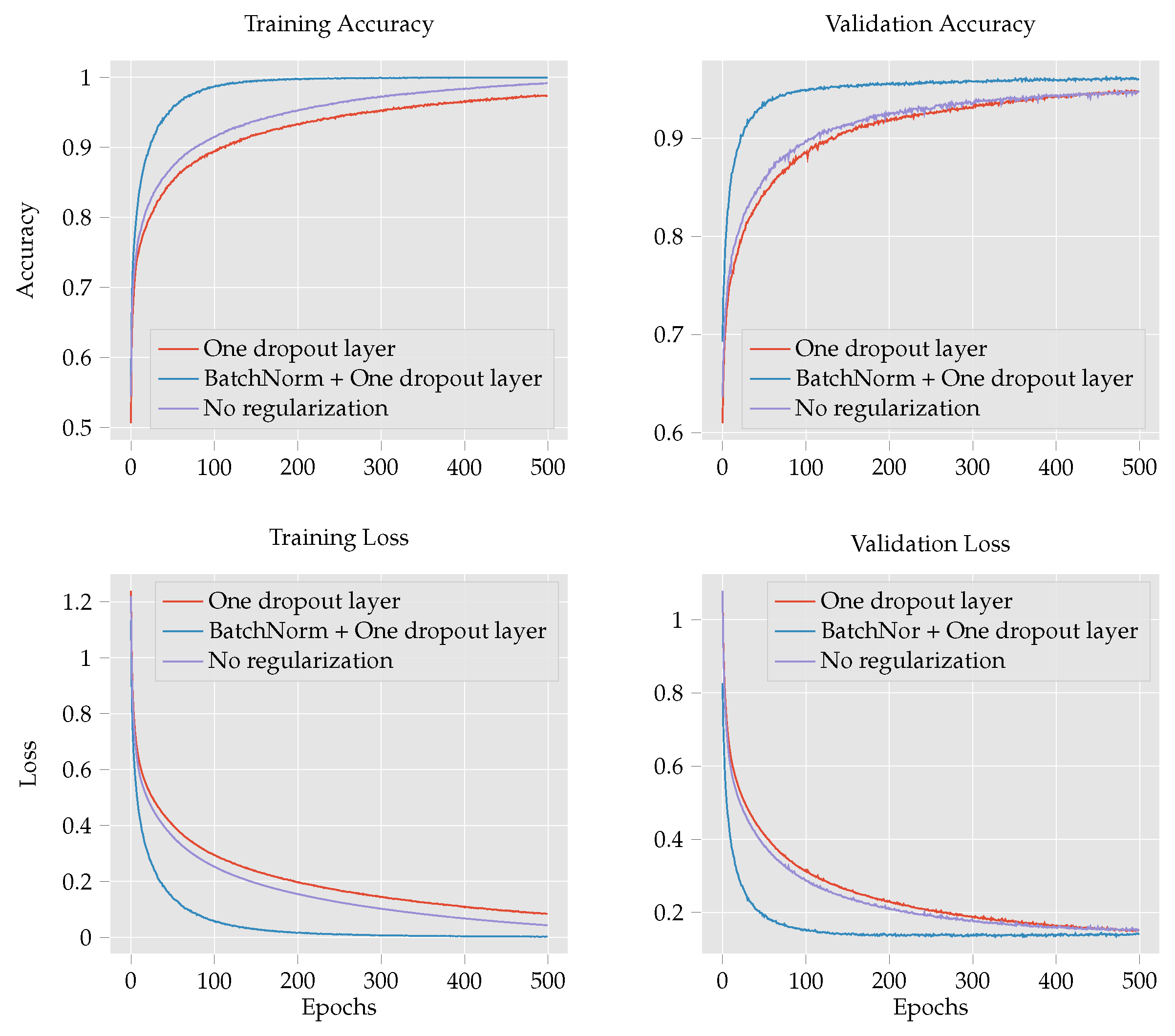
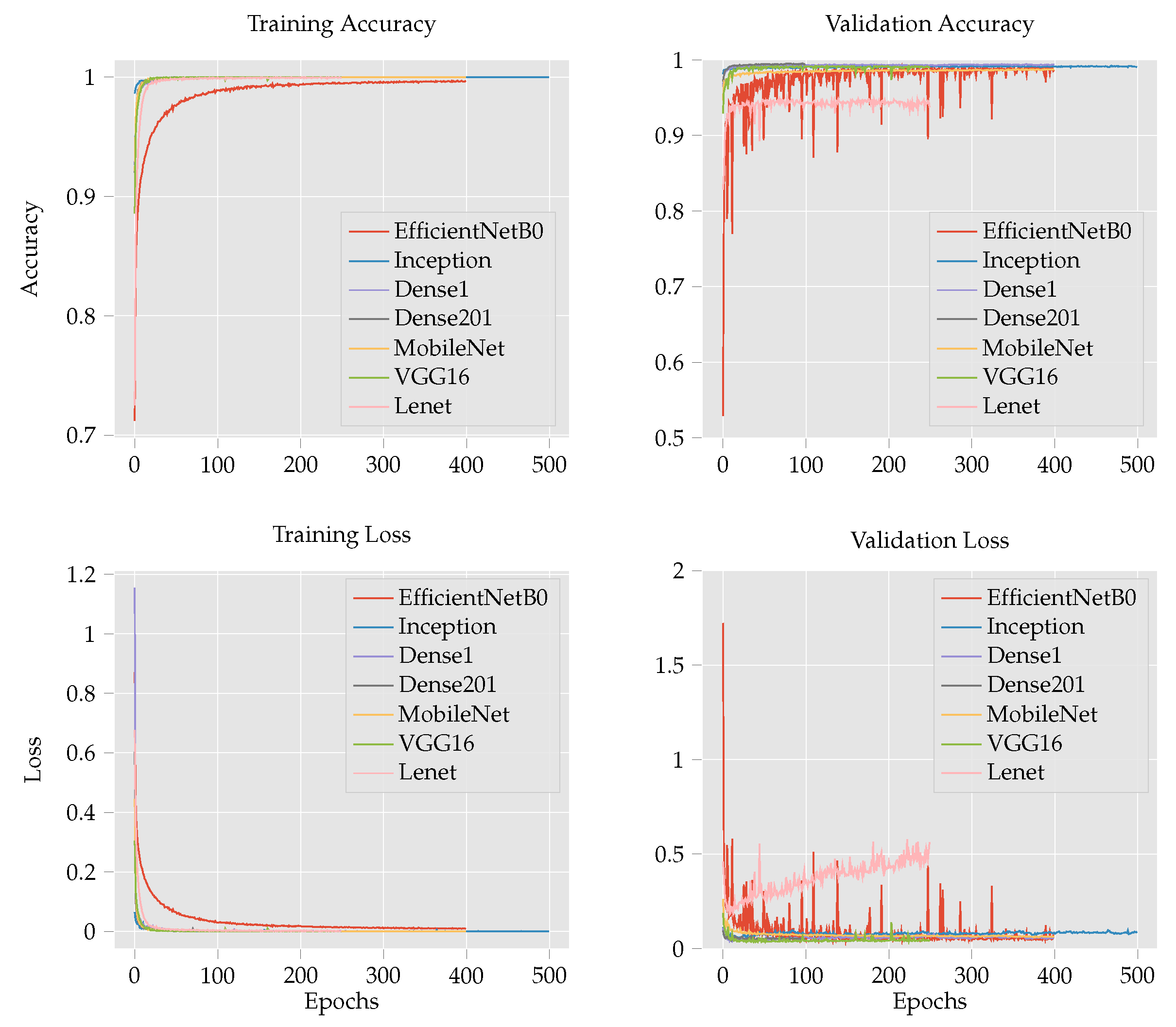
- To improve the classification accuracy of maize leaf disease identification, this work investigates several models: custom CNN, Inception V3 [15], DenseNet 121 [16], DenseNet 201 [16], MobileNetV2 [17], VGG16 [18], EffcientNetB0 [19], ResNet50 [20] and LeNet [21]. The performance of the custom CNN is further examined by comparing the effect of regularization techniques such as batch normalization and dropout operations. Finally, we compare the experimental results of the custom CNN with those of the transfer learning techniques to determine the effect of CNN depth and number parameters on the performance of the model.
- We propose a unique and computationally efficient adaptive thresholding method for quantifying the diseased regions of leaf images in an unsupervised manner. The advantage of this method is that it uses spatial relationships between the pixels to predict regions that are affected by the disease.
- Experimental results on the dataset demonstrate two things. First, the transfer learning techniques achieve higher classification accuracies of 99%. Second, our proposed adaptive thresholding approach performs well, giving good results, and therefore is a good approach for maize leaf disease quantification.
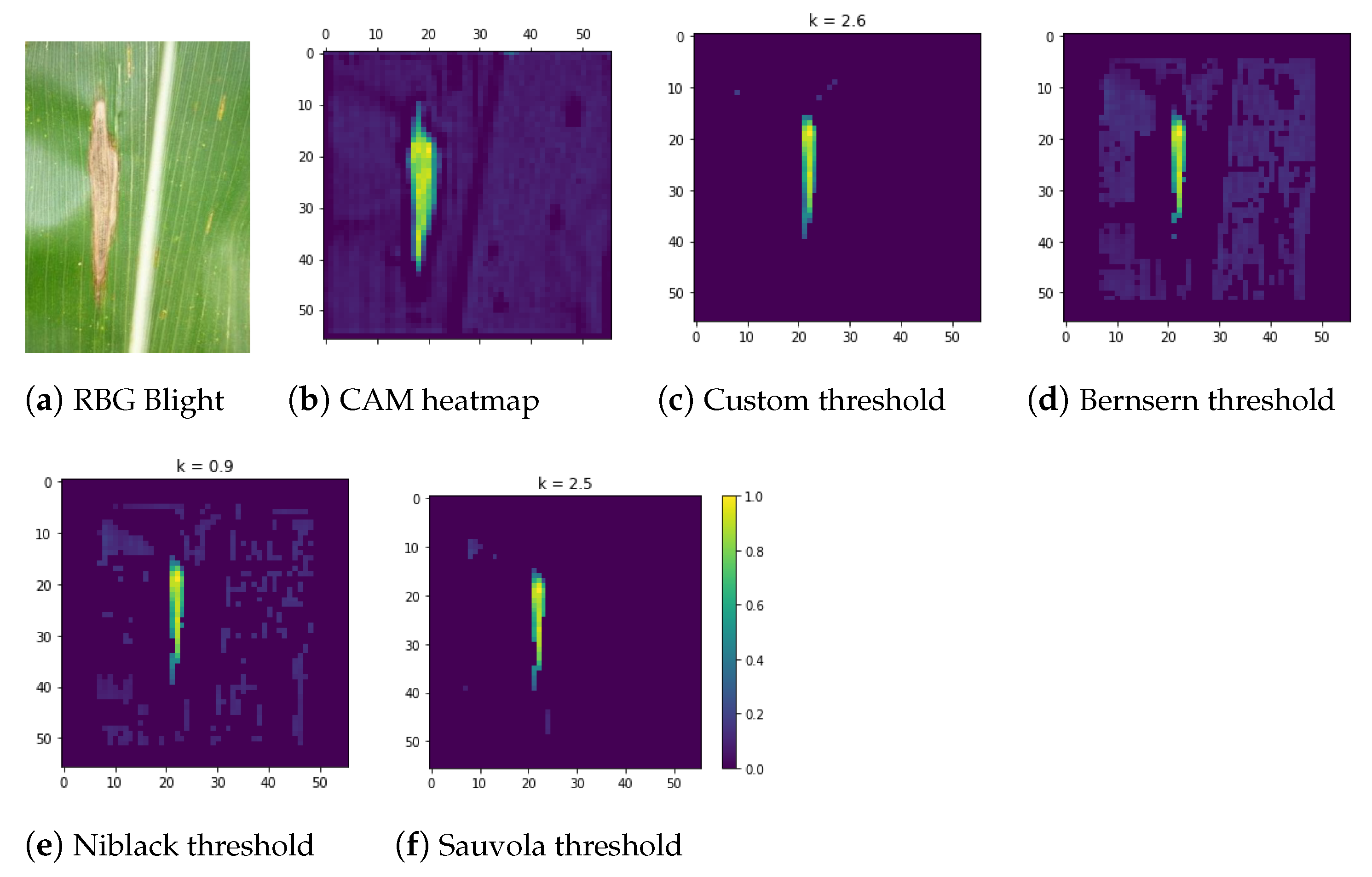
- Comparison evaluation with the most common maize leaf disease severity analyses such as Bernsern’s, Niblack’s and Sauvola’s thresholding reveal that our approach is robust and gives good results.
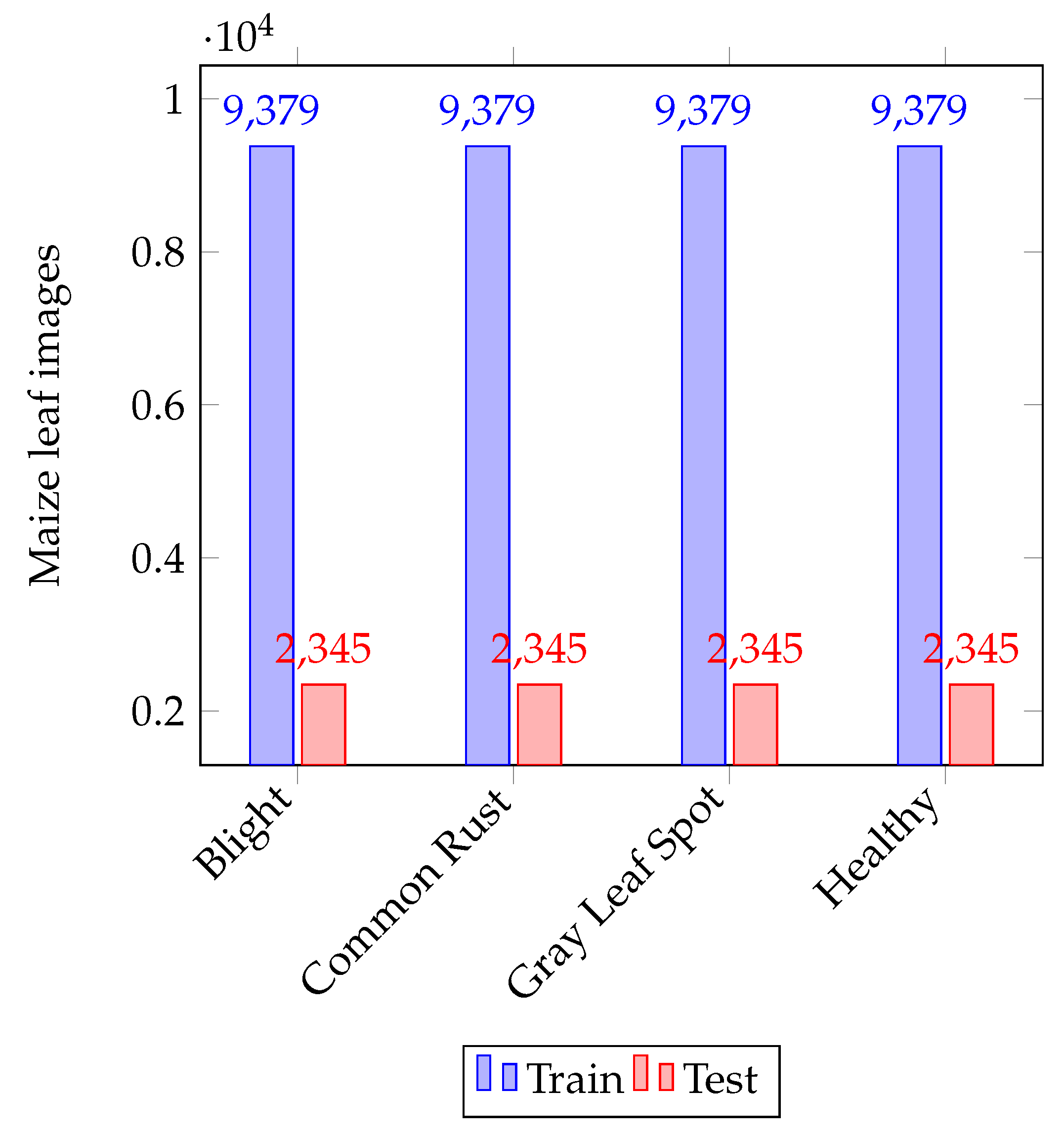
- We created an augmented dataset consisting of 46,898 samples from the original PlantVillage [22] dataset, available at: https://github.com/harryD1/maize_leaf_diseases_classification_and_quantification (accessed on 1 June 2022).
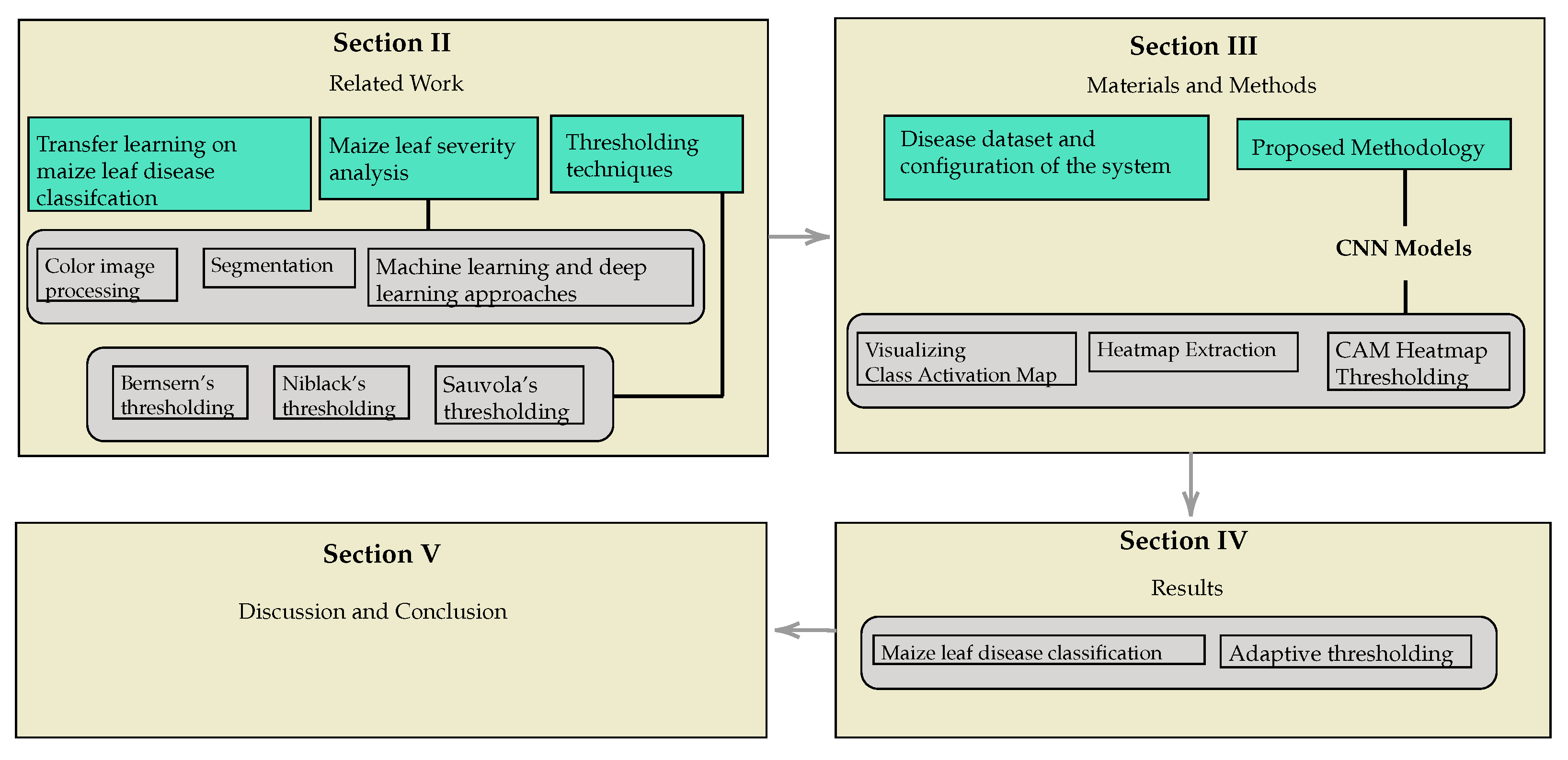
2. Related Work
2.1. Transfer Learning on Maize Leaf Disease Classification
2.2. Maize Leaf Severity Analysis
2.2.1. Color Image Processing
2.2.2. Segmentation
2.2.3. Machine Learning and Deep Learning
3. Materials and Methods
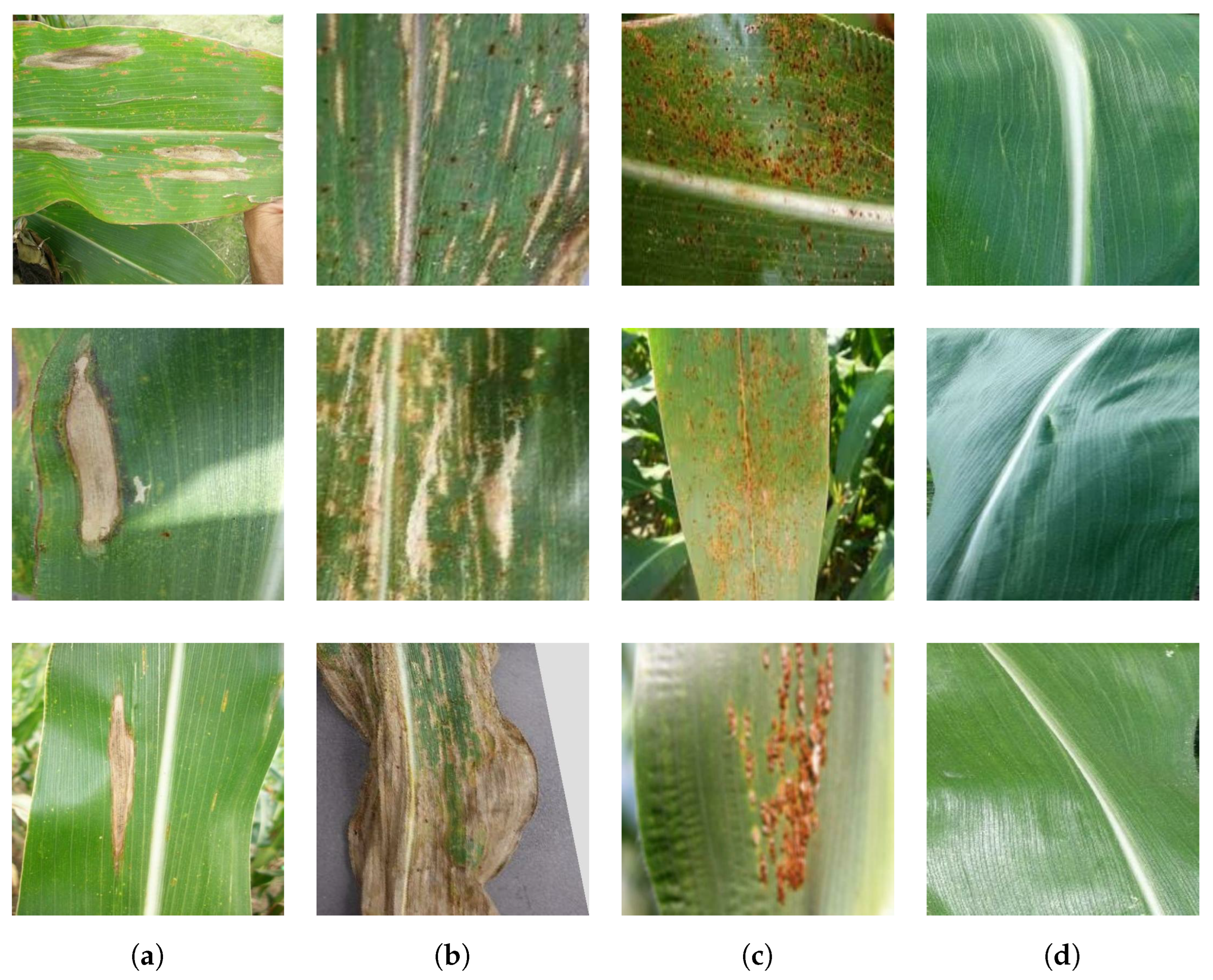
3.1. Disease Dataset and Configuration of the System
- Resizing—();
- Shear—level ;
- Rotation—90 degrees;
- Flipping—up_down flip;
- Saturation;
- Mean filtering;
- Flipping meaned image;
- Cropping—central_fraction = 0.8;
- Cropping—central_fraction = 0.5.
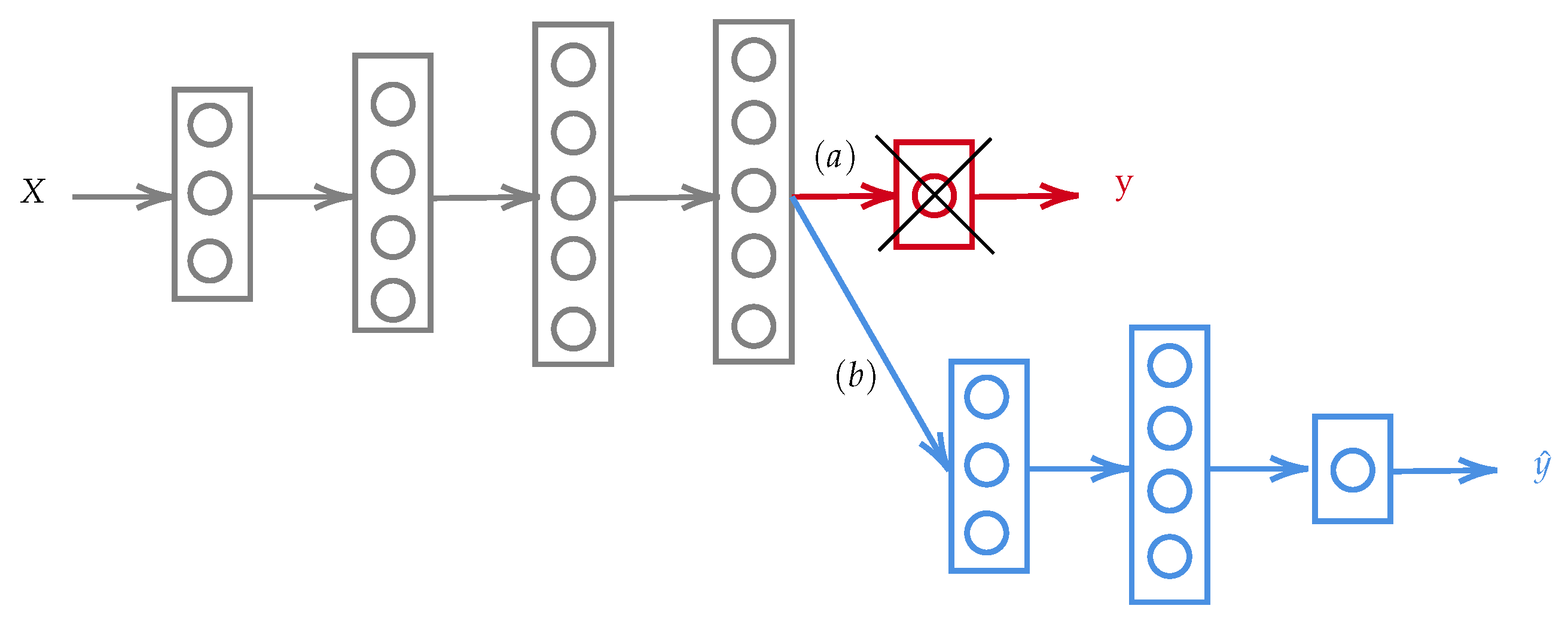
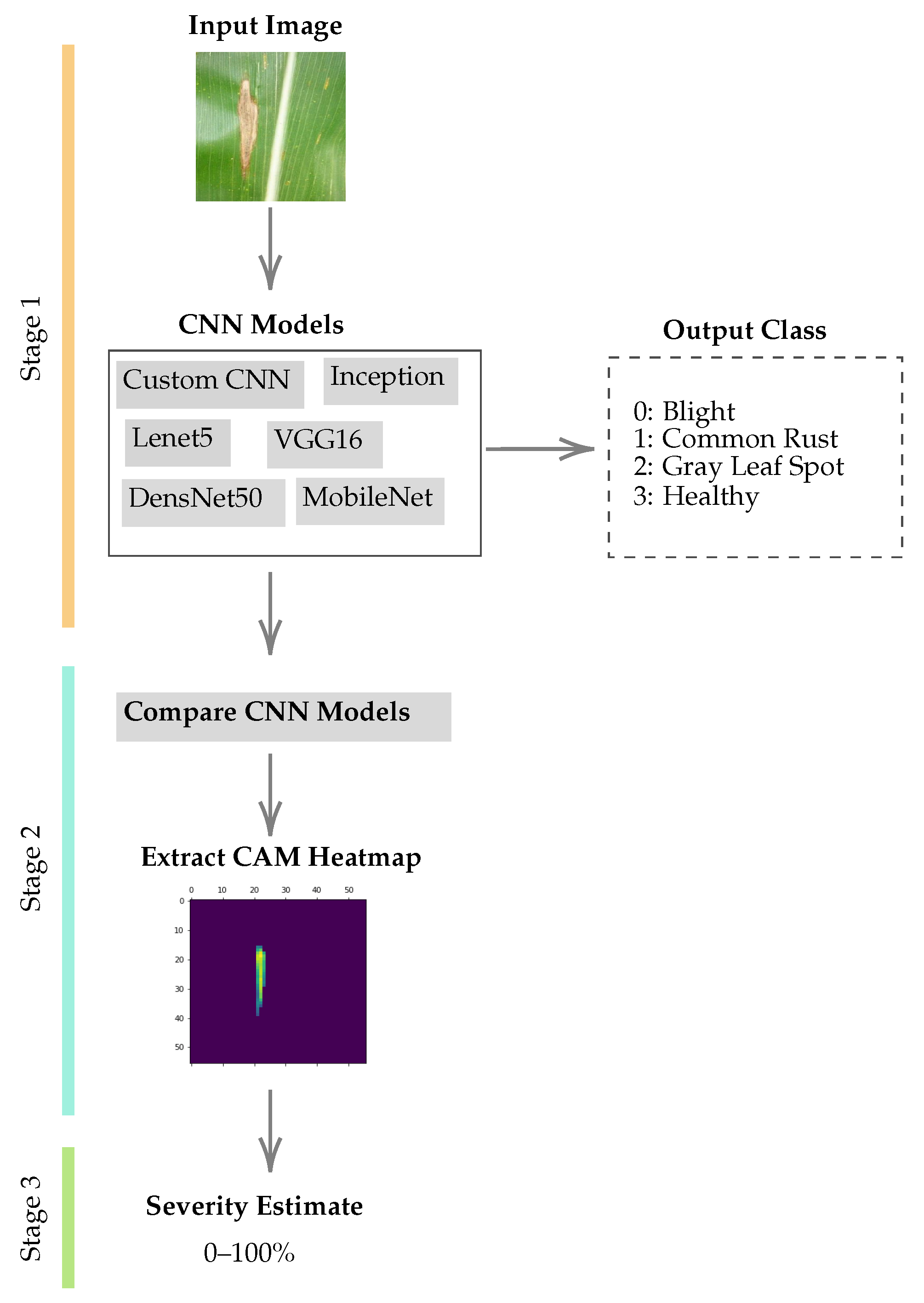
3.2. Proposed Methodology
- Step 1:
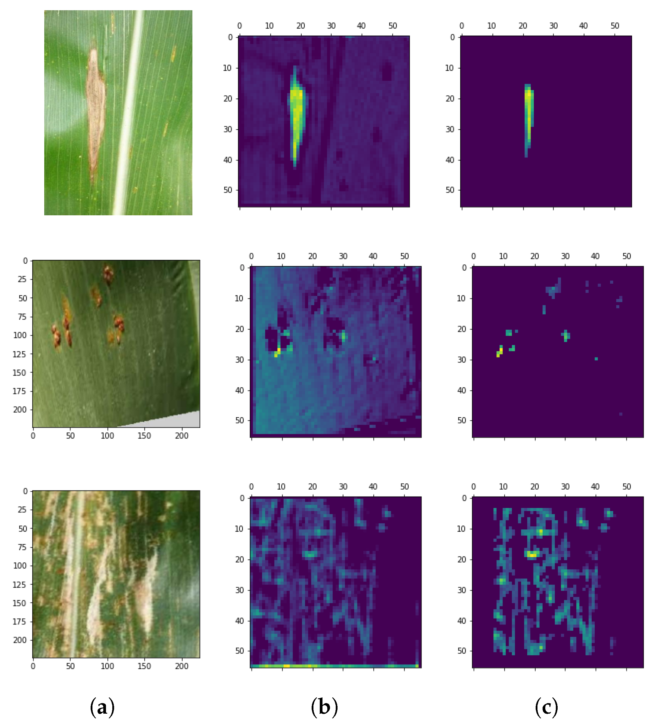
- We train a wide variety of well-known deep learning models for the maize leaf disease classification problem. Then, we compare the performance of the deep learning models and extract the class activation heatmaps from the prediction layers of the CNN models.
- Step 2:
- We extract the class activation heatmap as a 2D matrix from the covnet layers and determine the area affected by the disease (region of interest).
- Step 3:
- We use these regions of interest to estimate image leaf disease severity.
3.2.1. Architecture of the Proposed CNN
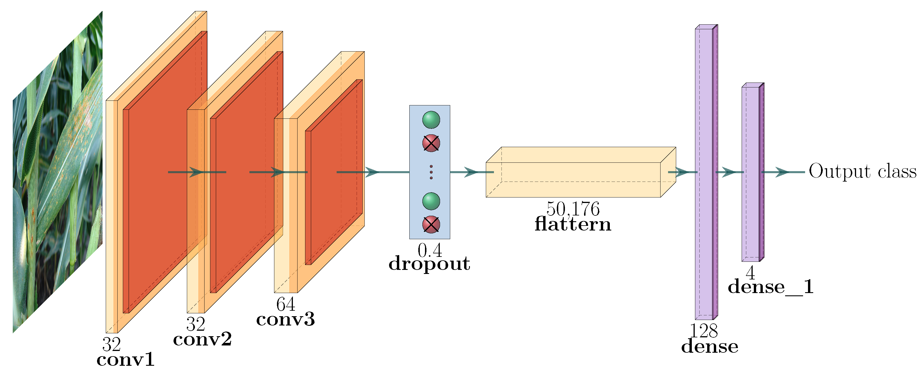
- Input image data: The images in our dataset have different sizes of width × height. However, the pre-processing stage of the CNN models resizes the images to a 3D matrix of . We have three channels since we are using RGB images.
- First hidden layer: The first hidden convolutional layer is called conv2d_1. It has 32 feature maps of size and a ReLu activation function.
- Second hidden layer: The second hidden layer is called conv2d_2. It has 32 feature maps of size and a ReLu activation function.
- Third hidden layer: Referred to as conv2d_3, it has 64 filters of size .
- Pooling layer: The pooling layer is called MaxPooling2D and is added after every convolutional layer.
- Dropout layer: A dropout layer is added to reduce overfitting; in this model, it has been set to exclude 30% of the neurons.
- Flatten layer: This layer is added to convert the 2D feature maps to a 1D vector.
- First fully connected layer: This has 128 neurons with a ReLu activation function.
- Output layer: This has four neurons and a softmax activation function.
3.2.2. Transfer Learning
3.2.3. State-of-the-Art Thresholding Techniques
Bernsern’s Thresholding
Niblack’s Thresholding
Sauvola’s Thresholding
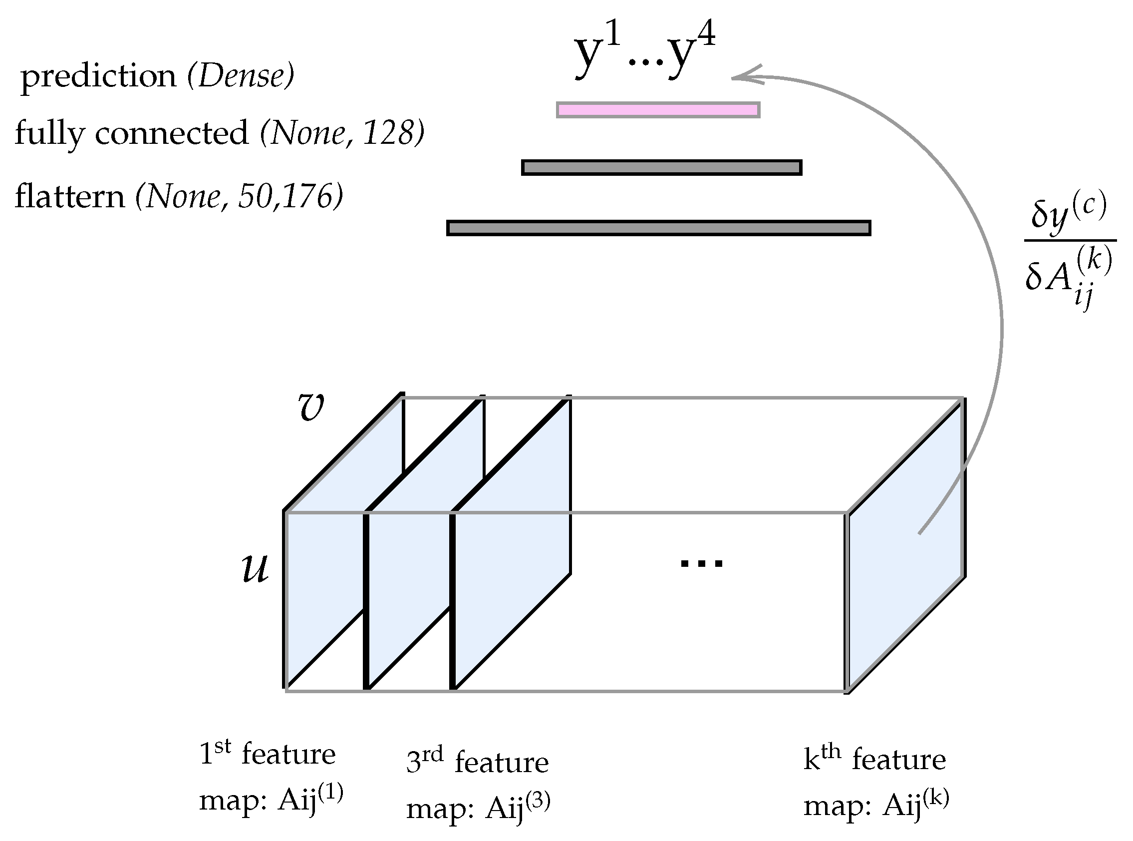
3.2.4. Visualizing the Class Activation Map (CAM)
3.2.5. Heatmap Extraction
3.2.6. Thresholding the Heatnap of the CAM
- is the adaptive threshold for each sliding window position;
- is the threshold factor;
- N is the number of samples in the sliding window;
- is the reference cell.
| Algorithm 1 Disease Extent Detection from CNN Heatmaps |
|
4. Results
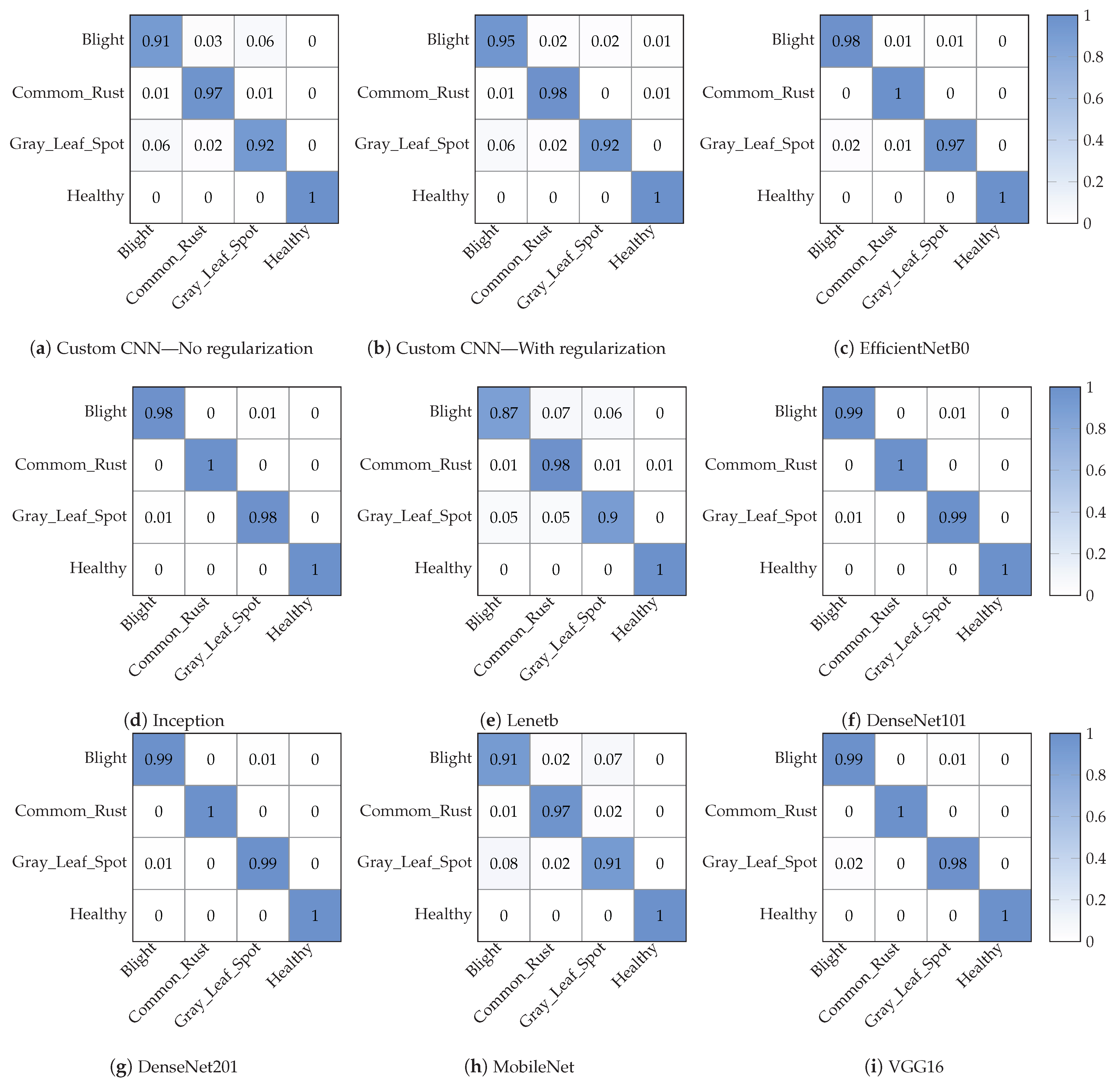
4.1. Maize Leaf Disease Classification
4.2. Adaptive Thresholding Performance
4.3. Leaf Disease Quantification
5. Discussion and Conclusions
Author Contributions
Funding
Data Availability Statement
Conflicts of Interest
Abbreviations
| CAM | Class Activation Map |
| CNN | Convolutional Neural Network |
| CUT | Cell Under Test |
| DL | Deep Learning |
| ML | Machine Learning |
| ROI | Region of Interest |
| SVM | Support Vector Machine |
References
- Food and Agriculture Organization of the United Nations. The Future of Food and Agriculture: Trends and Challenges. Available online: http://worldcat.org (accessed on 20 February 2022).
- Barburiceanu, S.; Meza, S.; Orza, B.; Malutan, R.; Terebes, R. Convolutional Neural Networks for Texture Feature Extraction. Applications to Leaf Disease Classification in Precision Agriculture. IEEE Access 2021, 9, 160085–160103. [Google Scholar] [CrossRef]
- Zhang, X.; Qiao, Y.; Meng, F.; Fan, C.; Zhang, M. Identification of Maize Leaf Diseases Using Improved Deep Convolutional Neural Networks. IEEE Access 2018, 6, 30370–30377. [Google Scholar] [CrossRef]
- Eraslan, G.; Avsec, Ž.; Gagneur, J.; Fabian, J. Deep learning: New computational modelling techniques for genomics. Nat. Rev. Genet. 2019, 20, 389–403. [Google Scholar] [CrossRef] [PubMed]
- Tetila, E.C.; Machado, B.B.; Menezes, G.K.; Junior, A.S.O.; Alvarez, M.; Amorim, W.P.; Belete, N.A.; Silva, G.G.; Pistori, H. Automatic Recognition of Soybean Leaf Diseases Using UAV Images and Deep Convolutional Neural Networks. IEEE Geosci. Remote Sens. Lett. 2020, 17, 903–907. [Google Scholar] [CrossRef]
- Taylor, B.; Marco, V.S.; Wolff, W.; Elkhatib, Y.; Wang, Z. Adaptive deep learning model selection on embedded systems. ACM Sigplan Not. 2018, 53, 31–43. [Google Scholar] [CrossRef]
- Lane, N.D.; Warden, P. The Deep (Learning) Transformation of Mobile and Embedded Computing. Computer 2018, 51, 12–16. [Google Scholar] [CrossRef]
- Dhingra, G.; Kumar, V.; Joshi, H.D. Study of digital image processing techniques for leaf disease detection and classification. Multimed. Tools Appl. 2018, 77, 19951–20000. [Google Scholar] [CrossRef]
- Bock, C.H.; Chiang, K.S.; Del Ponte, E.M. Plant disease severity estimated visually: A century of research, best practices, and opportunities for improving methods and practices to maximize accuracy. Trop. Plant Pathol. 2021, 47, 25–42. [Google Scholar] [CrossRef]
- Olivoto, T.; Andrade, S.; Del Ponte, E.M. Measuring plant disease severity in R: Introducing and evaluating the pliman package. Trop. Plant Pathol. 2022, 47, 95–104. [Google Scholar] [CrossRef]
- Owomugisha, G.; Ernest, M. Machine Learning for Plant Disease Incidence and Severity Measurements from Leaf Images. In Proceedings of the 2016 15th IEEE International Conference on Machine Learning and Applications (ICMLA), Anaheim, CA, USA, 18–20 December 2016; pp. 158–163. [Google Scholar] [CrossRef]
- Sethy, P.K.; Negi, B.; Barpanda, N.K.; Behera, S.K.; Rath, A.K. Measurement of Disease Severity of Rice Crop Using Machine Learning and Computational Intelligence. In Cognitive Science and Artificial Intelligence; SpringerBriefs in Applied Sciences and Technology; Springer: Singapore, 2017. [Google Scholar] [CrossRef]
- Liang, Q.; Xiang, S.; Hu, Y.; Coppola, G.; Zhang, D.; Sun, W. PD2SE-Net: Computer-assisted plant disease diagnosis and severity estimation network. Comput. Electron. Agric. 2019, 157, 518–529. [Google Scholar] [CrossRef]
- Kim, D.H.; Baddar, W.J.; Jang, J.; Ro, Y.M. Multi-Objective Based Spatio-Temporal Feature Representation Learning Robust to Expression Intensity Variations for Facial Expression Recognition. IEEE Trans. Affect. Comput. 2019, 10, 223–236. [Google Scholar] [CrossRef]
- Szegedy, C.; Vanhoucke, V.; Ioffe, S.; Shlens, J.; Wojna, Z. Rethinking the Inception Architecture for Computer Vision. In Proceedings of the IEEE Conference on Computer Vision and Pattern Recognition, CVPR 2016, Las Vegas, NV, USA, 27–30 June 2016; pp. 2818–2826. [Google Scholar] [CrossRef]
- Huang, G.; Liu, Z.; Van Der Maaten, L.; Weinberger, K.Q. Densely Connected Convolutional Networks. In Proceedings of the 2017 IEEE Conference on Computer Vision and Pattern Recognition (CVPR), Honolulu, HI, USA, 21–26 July 2017; pp. 2261–2269. [Google Scholar] [CrossRef]
- Sandler, M.; Howard, A.; Zhu, M.; Zhmoginov, A.; Chen, L.C. MobileNetV2: Inverted Residuals and Linear Bottlenecks. In Proceedings of the 2018 IEEE/CVF Conference on Computer Vision and Pattern Recognition, Salt Lake City, UT, USA, 18–23 June 2018; pp. 4510–4520. [Google Scholar] [CrossRef]
- Simonyan, K.; Andrew, Z. Very deep convolutional networks for large-scale image recognition. In Proceedings of the ICLR 2015 Conference, San Diego, CA, USA, 7–9 May 2015. [Google Scholar] [CrossRef]
- Tan, M.; Quoc, L. Efficientnet: Rethinking model scaling for convolutional neural networks. In Proceedings of the 36th International Conference on Machine Learning, PMLR 97, Long Beach, CA, USA, 9–15 June 2019; pp. 6105–6114. Available online: https://proceedings.mlr.press/v97/tan19a.html (accessed on 11 August 2021).
- He, K.; Zhang, S.; Ren, S.; Sun, J. Deep Residual Learning for Image Recognition. In Proceedings of the 2016 IEEE Conference on Computer Vision and Pattern Recognition (CVPR), Las Vegas, NV, USA, 27–30 June 2016; pp. 770–778. [Google Scholar] [CrossRef]
- Lecun, Y.; Bottou, L.; Bengio, Y.; Haffner, P. Gradient-based learning applied to document recognition. Proc. IEEE 1998, 86, 2278–2324. [Google Scholar] [CrossRef]
- Available online: https://github.com/spMohanty/PlantVillage-Dataset (accessed on 9 February 2020).
- Zhuang, F.; Qi, Z.; Duan, K.; Xi, D.; Zhu, Y.; Zhu, H.; Xiong, H.; He, Q. A Comprehensive Survey on Transfer Learning. Proc. IEEE 2020, 109, 43–76. [Google Scholar] [CrossRef]
- Panigrahi, K.P.; Das, H.; Sahoo, A.K.; Moharana, S.C. Maize Leaf Disease Detection and Classification Using Machine Learning Algorithms. In Progress in Computing, Analytics and Networking; Advances in Intelligent Systems and Computing; Das, H., Pattnaik, P., Rautaray, S., Li, K.C., Eds.; Springer: Singapore, 2020; Volume 1119. [Google Scholar] [CrossRef]
- Alehegn, E. Ethiopian maize diseases recognition and classification using support vector machine. Int. J. Comput. Vis. Robot. 2019, 9, 90–109. [Google Scholar] [CrossRef]
- Pantazi, X.E.; Moshou, D.; Tamouridou, A.A. Automated leaf disease detection in different crop species through image features analysis and One Class Classifiers. Comput. Electron. Agric. 2019, 156, 96–104. [Google Scholar] [CrossRef]
- Jayme, G.; Arnal, B. A review on the main challenges in automatic plant disease identification based on visible range images. Biosyst. Eng. 2016, 144, 52–60. [Google Scholar] [CrossRef]
- Shanwen, Z.; Xiaowei, W.; Zhuhong, Y.; Liqing, Z. Leaf image based cucumber disease recognition using sparse representation classification. Comput. Electron. Agric. 2017, 134, 135–141. [Google Scholar] [CrossRef]
- Ali, H.; Lali, M.I.; Nawaz, M.Z.; Sharif, M.; Saleem, B.A. Symptom based automated detection of citrus diseases using color histogram and textural descriptors. Comput. Electron. Agric. 2017, 138, 92–104. [Google Scholar] [CrossRef]
- Ordonez, F.J.; Roggen, D. Deep Convolutional and LSTM Recurrent Neural Networks for Multimodal Wearable Activity Recognition. Sensors 2016, 16, 115. [Google Scholar] [CrossRef]
- DeChant, C.; Wiesner-Hanks, T.; Chen, S.; Stewart, E.L.; Yosinski, J.; Gore, M.A.; Nelson, R.J.; Lipson, H. Automated Identification of Northern Leaf Blight-Infected Maize Plants from Field Imagery Using Deep Learning. Phytopathology 2017, 107, 1426–1432. [Google Scholar] [CrossRef]
- Feng, J.; Yang, L.; Yu, C.; Di, C.; Gongfa, L. Image recognition of four rice leaf diseases based on deep learning and support vector machine. Comput. Electron. Agric. 2020, 179, 105824. [Google Scholar] [CrossRef]
- Mohammad, S.; Wahyudi, S. Convolutional neural network for maize leaf disease image classification. Telkomnika 2020, 18, 1376–1381. [Google Scholar] [CrossRef]
- Zhou, C.; Zhou, S.; Xing, J.; Song, J. Tomato Leaf Disease Identification by Restructured Deep Residual Dense Network. IEEE Access 2021, 9, 28822–28831. [Google Scholar] [CrossRef]
- Liu, B.; Yu, X.; Zhang, P.; Yu, A.; Fu, Q.; Wei, X. Supervised Deep Feature Extraction for Hyperspectral Image Classification. IEEE Trans. Geosci. Remote Sens. 2018, 56, 1909–1921. [Google Scholar] [CrossRef]
- Barbedo, J.; Garcia, a. Impact of dataset size and variety on the effectiveness of deep learning and transfer learning for plant disease classification. Comput. Electron. Agric. 2017, 153, 46–53. [Google Scholar] [CrossRef]
- Bock, C.H.; Pethybridge, S.J.; Barbedo, J.G.; Esker, P.D.; Mahlein, A.K.; Del Ponte, E.M. A phytopathometry glossary for the twenty-first century: Towards consistency and precision in intra-and inter-disciplinary dialogues. Trop. Plant Pathol. 2022, 47, 14–24. [Google Scholar] [CrossRef]
- Bock, C.H.; Barbedo, J.G.A.; Del Ponte, E.M.; Bohnenkamp, D.; Mahlein, A. From visual estimates to fully automated sensor-based measurements of plant disease severity: Status and challenges for improving accuracy. Phytopathol. Res. 2020, 2, 9. [Google Scholar] [CrossRef]
- Arnal Barbedo, J.G. Digital image processing techniques for detecting, quantifying and classifying plant diseases. Springerplus 2013, 47, 14–24. [Google Scholar] [CrossRef]
- Barbora, S.; Vlastimil, K.; Rostislav, Z. Computer-assisted estimation of leaf damage caused by spider mites. Comput. Electron. Agric. 2006, 53, 81–91. [Google Scholar] [CrossRef]
- Sengar, N.; Malay, K.D.; Carlos, M.T. Computer vision based technique for identification and quantification of powdery mildew disease in cherry leaves. Computing 2018, 100, 1189–1201. [Google Scholar] [CrossRef]
- Saxena, D.K.; Jhanwar, D.; Gautam, D. Classification of Leaf Disease on Using Triangular Thresholding Method and Machine Learning. In Optical and Wireless Technologies. Lecture Notes in Electrical Engineering; Tiwari, M., Maddila, R.K., Garg, A.K., Kumar, A., Yupapin, P., Eds.; Springer: Singapore, 2022; Volume 771. [Google Scholar] [CrossRef]
- Bakar, M.N.; Abdullah, A.H.; Rahim, N.A.; Yazid, H.; Misman, S.N.; Masnan, M.J. Rice leaf blast disease detection using multi-level colour image thresholding. J. Telecommun. Electron. Comput. Eng. 2018, 10, 1–15. [Google Scholar]
- Sinha, A.; Shekhawat, R.S. Detection, Quantification and Analysis of Neofabraea Leaf Spot in Olive Plant using Image Processing Techniques. In Proceedings of the 2019 5th International Conference on Signal Processing, Computing and Control (ISPCC), Solan, India, 10–12 October 2019; pp. 348–353. [Google Scholar] [CrossRef]
- Yadav, A.; Dutta, M.K. An Automated Image Processing Method for Segmentation and Quantification of Rust Disease in Maize Leaves. In Proceedings of the 2018 4th International Conference on Computational Intelligence and Communication Technology (CICT), Ghaziabad, India, 9–10 February 2018; pp. 1–5. [Google Scholar] [CrossRef]
- Mahmud, A.; Esakki, B.; Seshathiri, S. Quantification of Groundnut Leaf Defects Using Image Processing Algorithms. In Advances in Intelligent Systems and Computing, Proceedings of the International Conference on Trends in Computational and Cognitive Engineering, Online, 21–22 October 2021; Springer: Singapore, 2021. [Google Scholar] [CrossRef]
- Barbedo, J.; Garcia, A. An automatic method to detect and measure leaf disease symptoms using digital image processing. Plant Dis. 2014, 98, 1709–1716. [Google Scholar] [CrossRef] [PubMed]
- Eaganathan, U.; Prasanna, S.; Sripriya, D. Various approaches of color feature extraction in leaf diseases under image processing: A survey. Int. J. Eng. Technol. 2018, 7, 712–717. [Google Scholar]
- Wilhelm, B.; Burge, M.J. Principles of Digital Image Processing Advanced Methods. Undergraduate Topics in Computer Science; Springer: London, UK, 2013. [Google Scholar] [CrossRef]
- Haris, I. PlotNeuralNet. Saarland University. Available online: https://github.com/HarisIqbal88/PlotNeuralNet (accessed on 10 December 2021).
- Bernsen, J. Dynamic thresholding of gray level images. In Proceedings of the International Conference on Pattern Recognition, Paris, France, 27–31 October 1986; pp. 1251–1255. [Google Scholar]
- Niblack, W. An introduction to Digital Image Processing; Prentice-Hall: Englewood Cliffs, NJ, USA, 1986; pp. 115–116. [Google Scholar]
- Sauvola, J.J.; Seppanen, T.; Haapakoski, S.; Pietikainen, M. Adaptive document binarization. In Proceedings of the 4th International Conference on Document Analysis and Recognition, Ulm, Germany, 18–20 August 1997; pp. 147–152. [Google Scholar]
- Sun, K.H.; Huh, H.; Tama, B.A.; Lee, S.Y.; Jung, J.H.; Lee, S. Vision-Based Fault Diagnostics Using Explainable Deep Learning with Class Activation Maps. IEEE Access 2020, 8, 129169–129179. [Google Scholar] [CrossRef]
- Richards, M.A. Fundamentals of Radar Signal Processing; McGraw-Hill Professional: New York, NY, USA, 2005. [Google Scholar]
- Abramoff, M.D.; Magalhaes, P.J.; Ram, S.J. Image processing with Image. J. Biophotonics 2004, 11, 36–42. [Google Scholar]


| CNN | ImageNet Accuracy | Layers | Params (M) |
|---|---|---|---|
| EfficientNetB0 | 77.1% | 132 | 5.3 |
| InceptionV3 | 77.9% | 189 | 23.9 |
| Lenet | 7 | 5.6 | |
| DenseNet121 | 75.0% | 242 | 8.1 |
| DenseNet201 | 77.3% | 402 | 20.2 |
| MobileNet | 70.4% | 55 | 4.3 |
| VGG16 | 71.3% | 16 | 138.4 |
| Custom CNN | – | 7 | 6.5 |
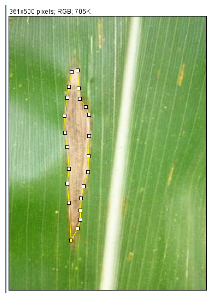
| Sample Image | % Area of the Diseased Region |
|---|---|
| ROI from the raw RGB leaf image | 4.87% |
| ROI extracted manually from the heatmap | 4.32% |
| ROI extracted from the heatmap using | 3.09% |
| our adaptive thresholding technique |
| Method | Class Label | Precision | Recall | F1-Score | Overall Accuracy |
|---|---|---|---|---|---|
| Inception V3 | Blight | 0.99 | 0.98 | 0.98 | 99% |
| Common Rust | 0.99 | 1.0 | 1.0 | ||
| Gray Leaf Spot | 0.99 | 0.98 | 0.98 | ||
| Healthy | 1.0 | 1.0 | 1.0 | ||
| DenseNet 121 | Blight | 0.99 | 0.99 | 0.99 | 99% |
| Common Rust | 1.00 | 1.00 | 1.00 | ||
| Gray Leaf Spot | 0.99 | 0.99 | 0.99 | ||
| Healthy | 1.00 | 1.00 | 1.00 | ||
| DenseNet 201 | Blight | 0.99 | 0.99 | 0.99 | 99% |
| Common Rust | 1.00 | 1.00 | 1.00 | ||
| Gray Leaf Spot | 0.99 | 0.99 | 0.99 | ||
| Healthy | 1.00 | 1.00 | 1.00 | ||
| MobileNet | Blight | 0.98 | 0.98 | 0.98 | 99% |
| Common Rust | 0.99 | 1.00 | 0.99 | ||
| Gray Leaf Spot | 0.98 | 0.98 | 0.98 | ||
| Healthy | 1.00 | 1.00 | 1.00 | ||
| VGG16 | Blight | 0.99 | 0.97 | 0.98 | 99% |
| Common Rust | 1.00 | 1.00 | 1.00 | ||
| Gray Leaf Spot | 0.97 | 0.99 | 0.98 | ||
| Healthy | 1.00 | 1.00 | 1.00 | ||
| EfficientNetB0 | Blight | 0.98 | 0.98 | 0.98 | 99% |
| Common Rust | 0.98 | 1.00 | 0.99 | ||
| Gray Leaf Spot | 0.98 | 0.97 | 0.98 | ||
| Healthy | 1.00 | 1.00 | 1000 | ||
| LeNet | Blight | 0.94 | 0.87 | 0.90 | 94% |
| Common Rust | 0.90 | 0.98 | 0.93 | ||
| Gray Leaf Spot | 0.93 | 0.90 | 0.92 | ||
| Healthy | 0.98 | 1.00 | 0.99 | ||
| Custom CNN (One dropout layer) | Blight | 0.92 | 0.92 | 0.92 | 95% |
| Common Rust | 0.96 | 0.96 | 0.96 | ||
| Gray Leaf Spot | 0.93 | 0.90 | 0.92 | ||
| Healthy | 0.97 | 1.00 | 0.99 | ||
| Custom CNN (Batch Nomarlization) | Blight | 0.93 | 0.95 | 0.94 | 96% |
| Common Rust | 0.96 | 0.98 | 0.97 | ||
| Gray Leaf Spot | 0.97 | 0.92 | 0.94 | ||
| Healthy | 0.98 | 1.00 | 0.99 | ||
| Custom CNN (No Regularization) | Blight | 0.92 | 0.91 | 0.92 | 95% |
| Common Rust | 0.94 | 0.97 | 0.96 | ||
| Gray Leaf Spot | 0.93 | 0.92 | 0.92 | ||
| Healthy | 0.99 | 1.00 | 1.00 |
Publisher’s Note: MDPI stays neutral with regard to jurisdictional claims in published maps and institutional affiliations. |
© 2022 by the authors. Licensee MDPI, Basel, Switzerland. This article is an open access article distributed under the terms and conditions of the Creative Commons Attribution (CC BY) license (https://creativecommons.org/licenses/by/4.0/).
Share and Cite
Mafukidze, H.D.; Owomugisha, G.; Otim, D.; Nechibvute, A.; Nyamhere, C.; Mazunga, F. Adaptive Thresholding of CNN Features for Maize Leaf Disease Classification and Severity Estimation. Appl. Sci. 2022, 12, 8412. https://0-doi-org.brum.beds.ac.uk/10.3390/app12178412
Mafukidze HD, Owomugisha G, Otim D, Nechibvute A, Nyamhere C, Mazunga F. Adaptive Thresholding of CNN Features for Maize Leaf Disease Classification and Severity Estimation. Applied Sciences. 2022; 12(17):8412. https://0-doi-org.brum.beds.ac.uk/10.3390/app12178412
Chicago/Turabian StyleMafukidze, Harry Dzingai, Godliver Owomugisha, Daniel Otim, Action Nechibvute, Cloud Nyamhere, and Felix Mazunga. 2022. "Adaptive Thresholding of CNN Features for Maize Leaf Disease Classification and Severity Estimation" Applied Sciences 12, no. 17: 8412. https://0-doi-org.brum.beds.ac.uk/10.3390/app12178412