


Performance Evaluation of Machine Learning Methods for Anomaly Detection in CubeSat Solar Panels

Abstract
:1. Introduction
- -
- Analysis of the novel solar panel dataset collected from four CubeSats.
- -
- Analysis of five different ML models based on their classification scores, execution times, model sizes, and power consumption.
- -
- The proposal of ML model candidates for solar panel anomaly detection on CubeSat systems.
2. Materials
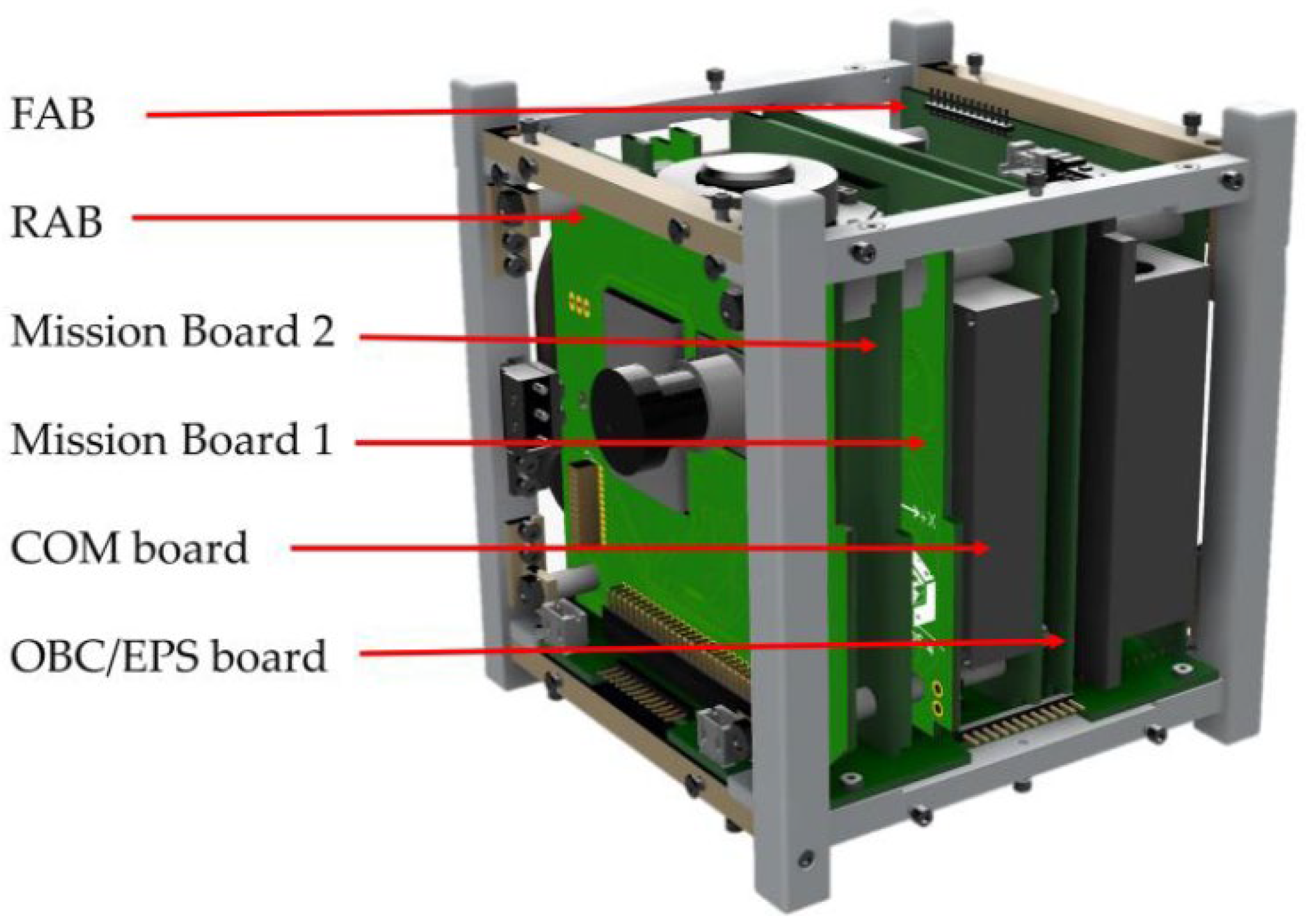
2.1. BIRDS Satellite System
2.2. Dataset Overview
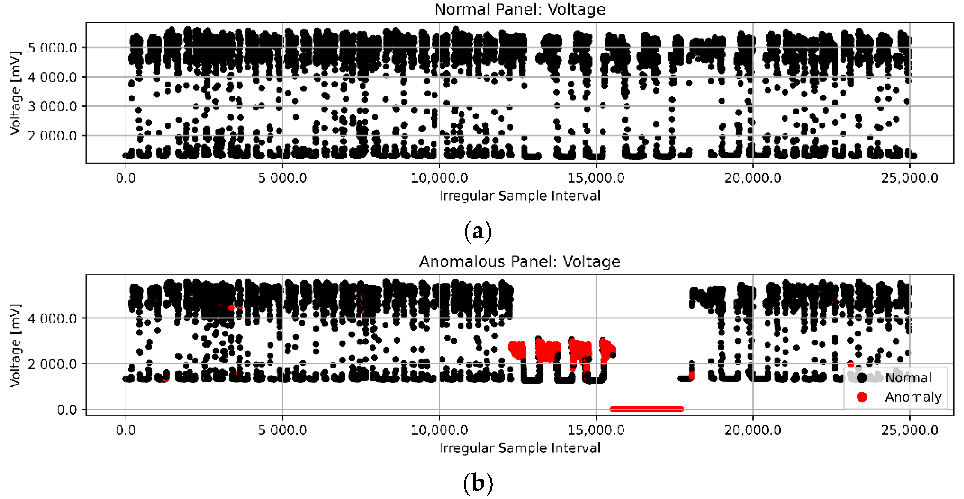
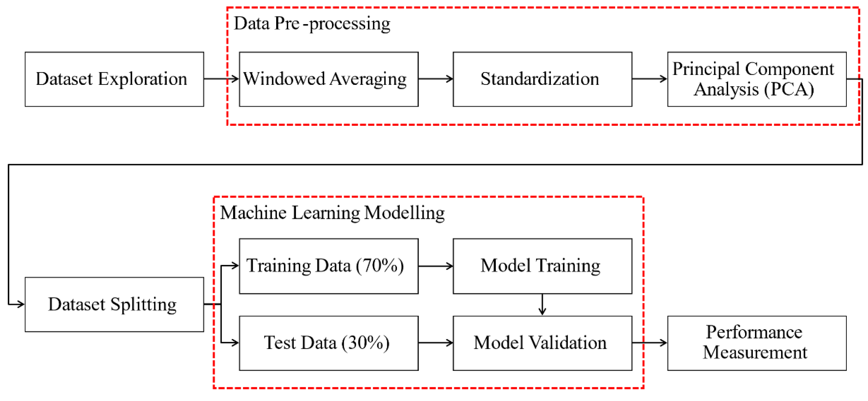
2.3. Data Exploration and Pre-Processing
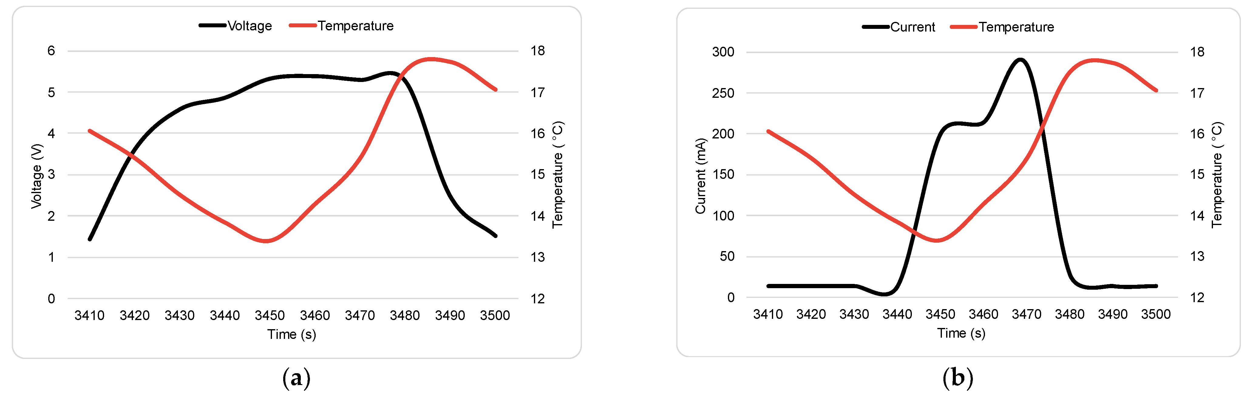
2.4. Dataset Correlation
3. Methods
3.1. Anomaly Definition
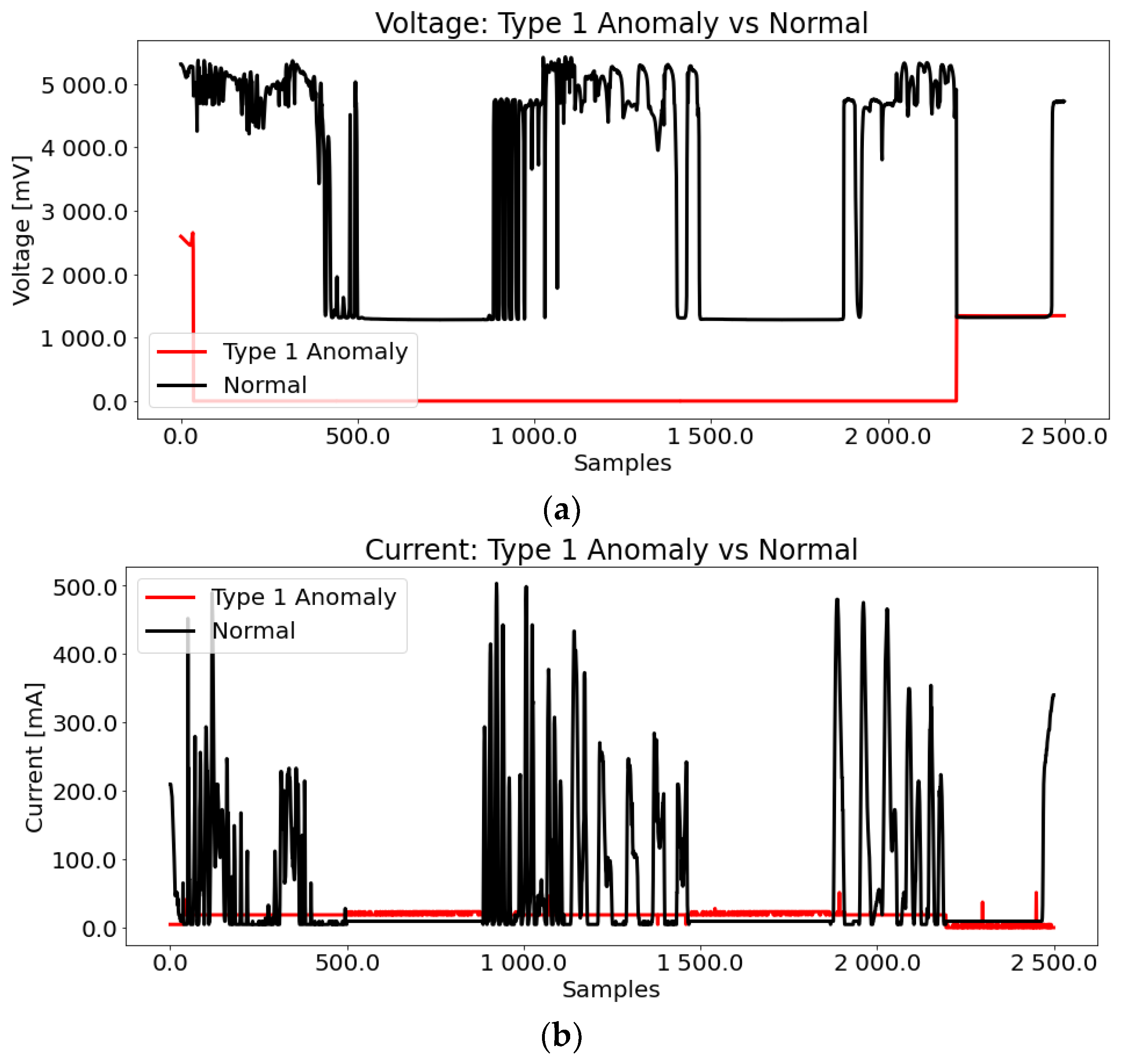
3.1.1. Type 1: Solar Panel Failure
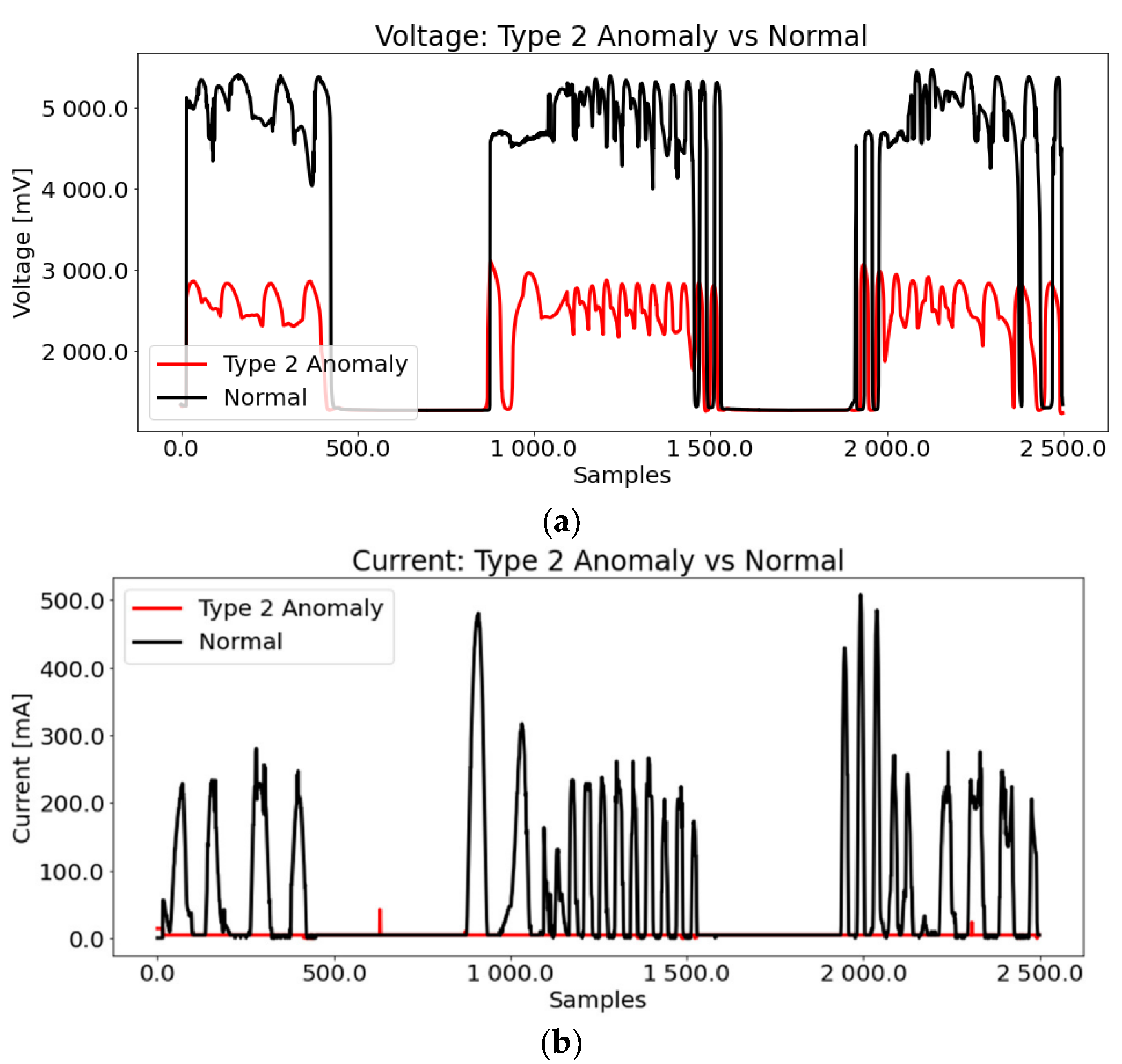
3.1.2. Type 2: Solar Cell Failure
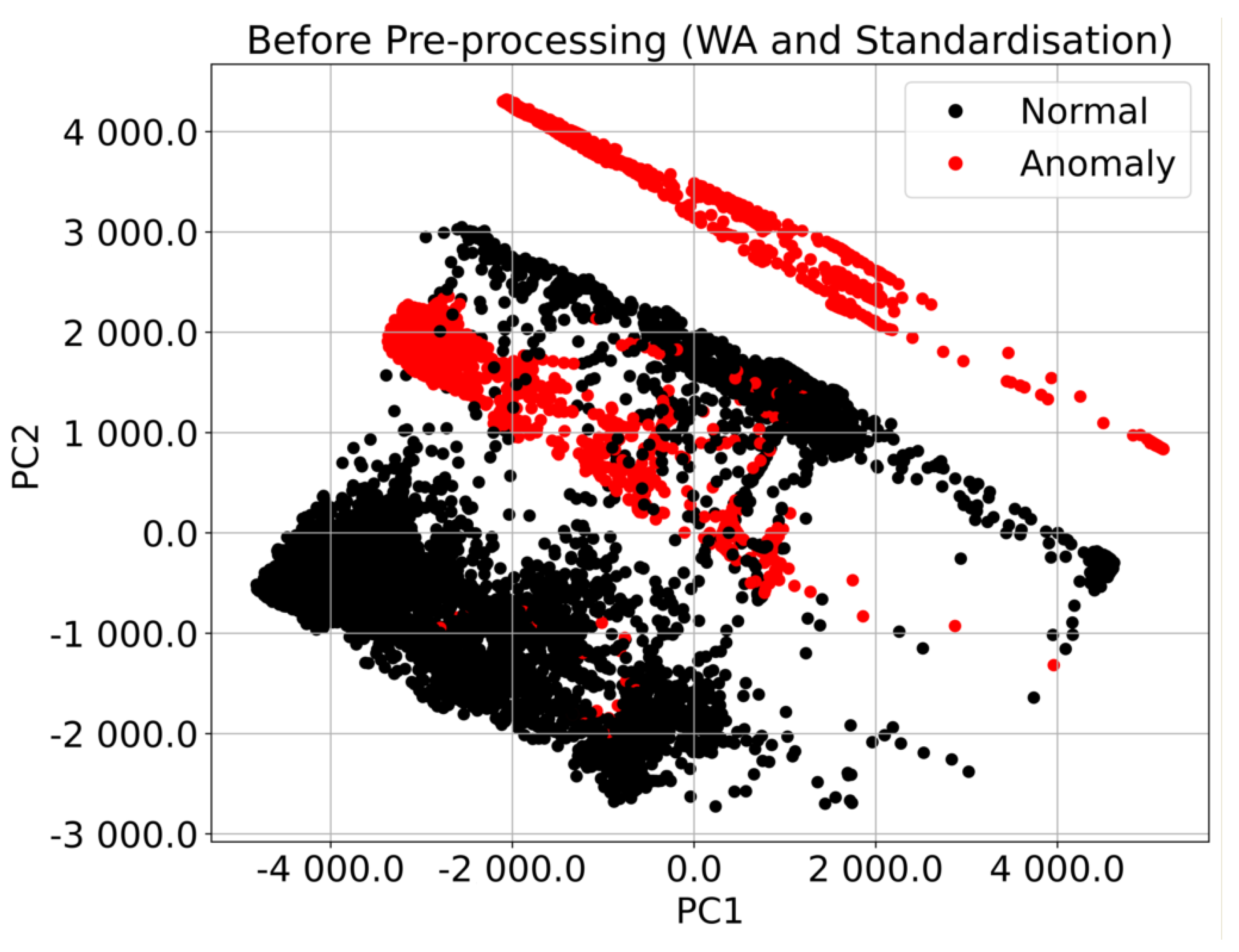
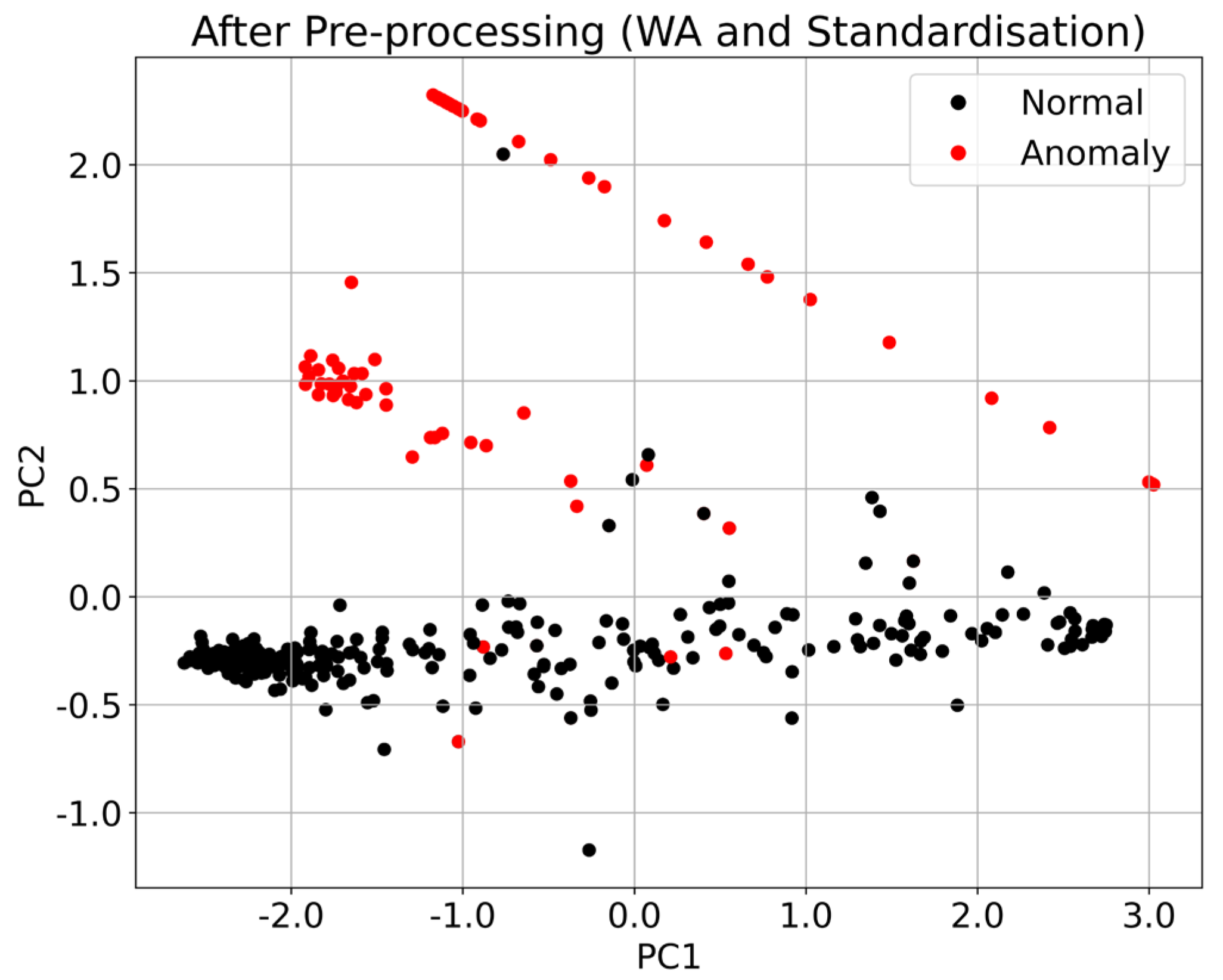
3.2. Pre-Processing Techniques
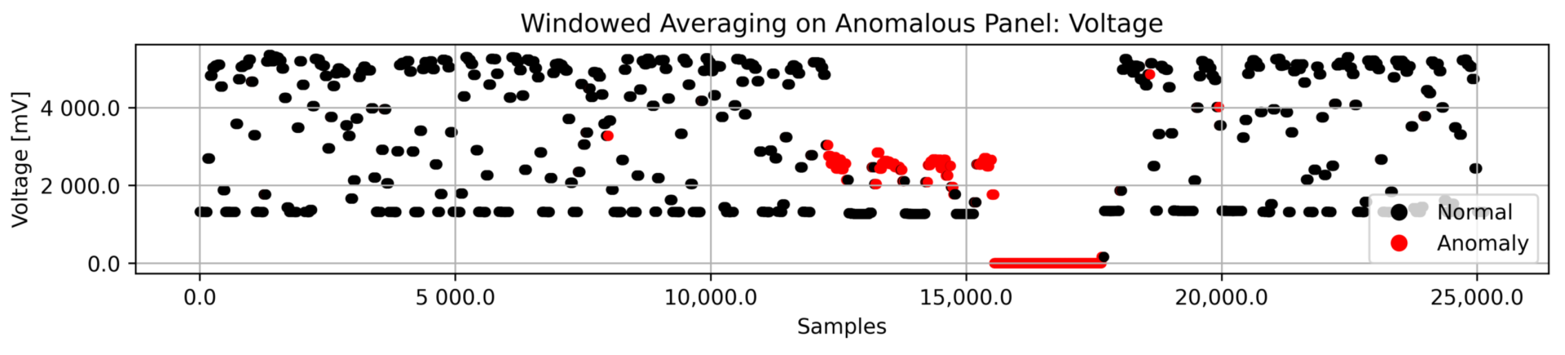
3.2.1. Windowed Averaging
3.2.2. Standardization
3.2.3. Principal Component Analysis
3.3. Model Candidates
3.3.1. Proximity-Based Algorithms
- A.
- Local Outlier Factor
- B.
- Cluster-Based Local Outlier Factor
- C.
- K-Nearest Neighbor
3.3.2. Linear Model
- A.
- Linear Discriminant Analysis
- B.
- One-Class Support Vector Machine
3.4. Experimental Setup
3.4.1. Environment and System
3.4.2. Simulation Parameters
4. Results
4.1. Performance Evaluation
4.2. Analysis
5. Discussion
6. Conclusions
Supplementary Materials
Author Contributions
Funding
Institutional Review Board Statement
Informed Consent Statement
Data Availability Statement
Acknowledgments
Conflicts of Interest
References
- BIRDS Program Digital Textbook CubeSTD-2019-001G. Available online: https://www.birds-project.com (accessed on 10 August 2021).
- Jara, A.; Bautista, I.; Maeda, G.; Kim, S.; Masui, H.; Yamauchi, T.; Cho, M. An Overview of the BIRDS-4 Satellite Project and the First Satellite of Paraguay. In Proceedings of the 35th Conference on Small Satellites, Logan, UT, USA, 7–12 August 2021. [Google Scholar]
- Cho, M.; Graziani, F. Definition and Requirements of Small Satellites Seeking Low-Cost and Fast-Delivery; IAA SG-2007-4.18; IAA: Paris, France, 2017. [Google Scholar]
- Wertz, J.R.; Everett, D.F.; Puschell, J.J. Space Mission Engineering: The New SMAD, 1st ed.; Microcosm Press: Hawthorne, CA, USA, 2011; pp. 45–59. [Google Scholar]
- Langer, M.; Bouwmeester, J. Reliability of CubeSats—Statistical Data, Developers’ Beliefs and the Way Forward. In Proceedings of the 30th Conference on Small Satellites, Logan, UT, USA, 6–11 August 2016. [Google Scholar]
- Maskey, A.; Cho, M. CubeSatNet: Ultralight Convolutional Neural Network designed for on-orbit binary image classification on a 1U CubeSat. Eng. Appl. Artif. Intell. 2020, 96, 103952. [Google Scholar] [CrossRef]
- Wu, J.; Yao, L.; Liu, B.; Ding, Z.; Zhang, L. Combining OC-SVMs With LSTM for Detecting Anomalies in Telemetry Data with Irregular Intervals. IEEE Access 2020, 8, 106648–106659. [Google Scholar] [CrossRef]
- Jin, W.; Sun, B.; Li, Z.; Zhang, S.; Chen, Z. Detecting Anomalies of Satellite Power Subsystem via Stage-Training Denoising Autoencoders. Sensors 2019, 19, 3216. [Google Scholar] [CrossRef]
- Yairi, T.; Takeishi, N.; Oda, T.; Nakajima, Y.; Nishimura, N.; Takata, N. A Data-Driven Health Monitoring Method for Satellite Housekeeping Data Based on Probabilistic Clustering and Dimensionality Reduction. IEEE Trans. Aerosp. Electr. Syst. 2017, 53, 1384–1401. [Google Scholar] [CrossRef]
- Zamry, N.M.; Zainal, A.; Rassam, M.A.; Alkhammash, E.H.; Ghaleb, F.A.; Saeed, F. Lightweight Anomaly Detection Scheme Using Incremental Principal Component Analysis and Support Vector Machine. Sensors 2021, 21, 8017. [Google Scholar] [CrossRef] [PubMed]
- Pan, D.; Liu, D.; Zhou, J.; Zhang, G. Anomaly detection for satellite power subsystem with associated rules based on Kernel Principal Component Analysis. Microelect. Reliab. 2015, 55, 2082–2086. [Google Scholar] [CrossRef]
- Peng, Y.; Jia, S.; Feng, X.; Su, F. Telemetry fault detection for meteorological satellite based on PCA. In Proceedings of the 16th International Symposium on Communications and Information Technologies, Qingdao, China, 8–10 December 2016. [Google Scholar]
- Li, J.; Yang, W.; Liu, D.; Liu, J. Kernel Self-Adaptive Learning-Based Satellite Telemetry Data Classification. In Proceedings of the 3rd International Conference on Computing Measurement Control and Sensor Network, Matsue, Japan, 20–22 May 2016. [Google Scholar]
- Umezu, R.; Sugie, T.; Nagase, M.; Kokai, R.; Takeshima, T.; Ebisawa, K.; Mitsuda, K.; Yamamoto, Y. Detection of Failure Sign of Spacecraft using Machine Learning. Space Sci. Inf. Japan 2019, 8, 11–20. [Google Scholar]
- BIRDS Open-Source Repository. Available online: https://github.com/BIRDSOpenSource (accessed on 13 March 2022).
- Chamika, D.; Cho, M.; Maeda, G.; Kim, S.; Masui, H.; Yamauchi, T.; Panawennage, S.; Shrestha, B. BIRDS-3 Satellite Project Including the First Satellites of Sri Lanka and Nepal. In Proceedings of the 70th International Astronautical Congress, Washington, DC, USA, 21 October 2019. [Google Scholar]
- Nakayama, D.; Yamauchi, T.; Masui, H.; Kim, S.; Toyoda, K.; Malmadayalage, T.L.D.; Cho, M.; the BIRDS-4 Project Team. On-Orbit Experimental Result of a Non-Deployable 430-MHz-Band Antenna Using a 1U CubeSat Structure. Electronics 2022, 11, 1163. [Google Scholar] [CrossRef]
- Pedregosa, F.; Varoquaux, G.; Gramfort, A.; Michel, V.; Thirion, B. Scikit-learn: Machine Learning in Python. J. Mach. Learn. Res. 2011, 12, 2825–2830. [Google Scholar]
- Kreyszig, E. Advanced Engineering Mathematics, 10th ed.; Wiley: Hoboken, NJ, USA, 2011; p. 880. [Google Scholar]
- Murphy, K. Machine Learning: A Probabilistic Perspective, 1st ed.; MIT Press: Cambridge, UK, 2012. [Google Scholar]
- Minka, T.P. Automatic choice of dimensionality for PCA. In Proceedings of the 2000 Neural Information Processing Systems (NIPS) Conference, Denver, CO, USA, 27 November–2 December 2000; Volume 13, pp. 598–604. [Google Scholar]
- Zhao, Y.; Nasrullah, Z.; Li, Z. PyOD: A Python Toolbox for Scalable Outlier Detection. J. Mach. Learn. Res. 2019, 20, 1–7. [Google Scholar]
- Goldstein, M.; Uchida, S. A Comparative Evaluation of Unsupervised Anomaly Detection Algorithms for Multivariate Data. PLoS ONE 2016, 11, e0152173. [Google Scholar] [CrossRef] [PubMed]
- Breunig, M.M.; Kriegel, H.P.; Raymond, T.; Sander, J. LOF: Identifying density-based local outliers. ACM Sig. Rec. 2000, 29, 93–104. [Google Scholar] [CrossRef]
- He, Z.; Xu, X.; Deng, S. Discovering cluster-based local outliers. Patt. Recog. Lett. 2003, 24, 1641–1650. [Google Scholar] [CrossRef]
- Ramaswamy, S.; Rastogi, R.; Shim, K. Efficient algorithms for mining outliers from large data sets. ACM Sig. Rec. 2000, 29, 427–438. [Google Scholar] [CrossRef]
- Duda, R.; Hart, P.; Stork, D. Pattern Classification, 2nd ed.; Wiley: Hoboken, NJ, USA, 2000; pp. 215–264. [Google Scholar]
- Scholkopf, B.; Platt, J.C.; Shawe-Taylor, J.; Smola, A.J.; Williamson, R.C. Estimating the Support of a High-dimensional Distribution. Neural Comp. 2001, 13, 1443–1471. [Google Scholar] [CrossRef] [PubMed]
- Kluyver, T.; Ragan-Kelley, B.; Pérez, F.; Granger, B.E.; Bussonnier, M.; Frederic, J.; Kelley, K.; Hamrick, J.B.; Grout, J.; Corlay, S.; et al. Jupyter Notebooks—A publishing format for reproducible computational workflows. In Positioning and Power in Academic, Players, Agents and Agendas; IOS Press: Amsterdam, The Netherlands, 2016; pp. 87–90. [Google Scholar]
- The Python Library Reference, Release 3.8.8, Python Software Foundation. Available online: https://www.python.org/downloads/release/python-388/ (accessed on 13 March 2021).
- Harris, C.R.; Millman, K.J.; van der Walt, S.J. Array programming with NumPy. Nature 2020, 585, 357–362. [Google Scholar] [CrossRef] [PubMed]
- McKinney, W. Data Structures for Statistical Computing in Python. In Proceedings of the 9th Python in Science Conference, Austin, TX, USA, 28 June 2010. [Google Scholar]
- Virtanen, P.; Gommers, R.; Oliphant, T.E. SciPy 1.0: Fundamental Algorithms for Scientific Computing in Python. Nat. Methods 2020, 17, 261–272. [Google Scholar] [CrossRef]
- Hunter, J.D. Matplotlib: A 2D Graphics Environment. IEEE Comput. Sci. Eng. 2007, 9, 90–95. [Google Scholar] [CrossRef]
- Reiinakano/Scikit-Plot: V0.3.5. Available online: https://zenodo.org/record/1245853#.Yogp4ujMJPY (accessed on 13 March 2021).
- Waskom, M.L. Seaborn: Statistical Data Visualization. J. Open Source Softw. 2021, 6, 3021. [Google Scholar] [CrossRef]
- Manning, C.D.; Raghavan, P.; Schütze, H. Introduction to Information Retrieval, 1st ed.; Cambridge University Press: Cambridge, UK, 2008; pp. 151–175. [Google Scholar]
- Sokolova, M.; Lapalme, G. A Systematic Analysis of Performance Measures for Classification Tasks. Inf. Process. Manag. 2009, 45, 427–437. [Google Scholar] [CrossRef]


| Sensor | Variable | Unit | Data Size |
|---|---|---|---|
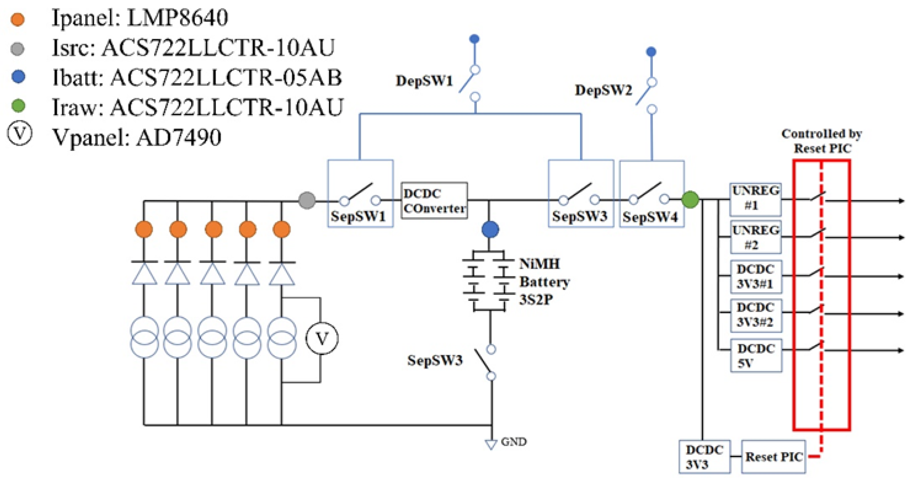
| LMP8640 | Current | mA | 8 bits |
| AD7490 | Voltage | mV | 12 bits |
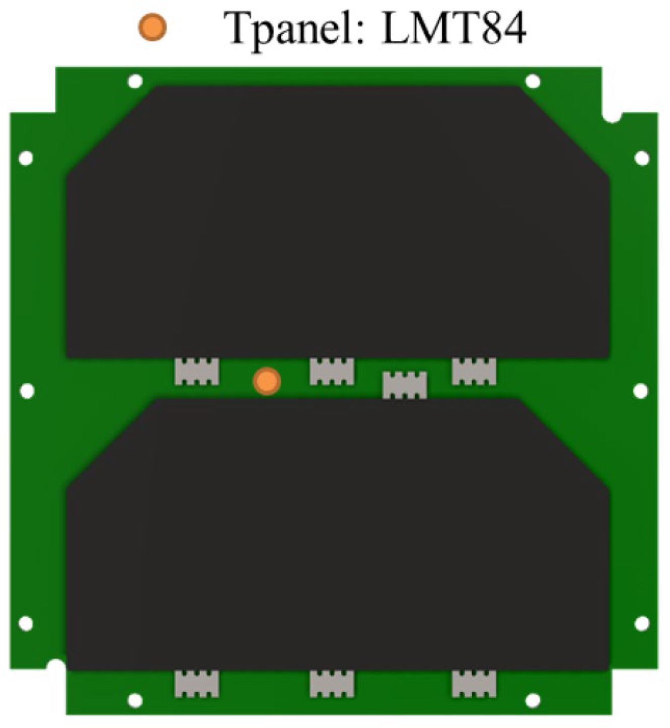
| LMT84 | Temperature | °C | 12 bits |
| Algorithm | Optimized Parameters | Trials | Best Value |
|---|---|---|---|
| Windowed Averaging | window size | 10–300 | 50 |
| PyOD Models | outlier fraction | 0.05–0.2 | 0.16 |
| kNN | neighbors | 10–300 | 255 |
| LOF | neighbors | 10–350 | 280 |
| Models | Precision * | Sensitivity * | F1-Score * |
|---|---|---|---|
| LOF | 0.26 ± 0.02 | 0.26 ± 0.03 | 0.26 ± 0.02 |
| CB-LOF | 0.64 ± 0.02 | 0.65 ± 0.02 | 0.64 ± 0.01 |
| kNN | 0.34 ± 0.01 | 0.34 ± 0.01 | 0.34 ± 0.01 |
| LDA | 0.97 ± 0.01 | 0.75 ± 0.01 | 0.85 ± 0.01 |
| OC-SVM | 0.83 ± 0.01 | 0.83 ± 0.02 | 0.83 ± 0.01 |
| Models | Execution Time [s] * | Model Size [kB] | Power Consumption [mWh] |
|---|---|---|---|
| LDA | 3.00 ± 0.17 | 40.17 | 4.288 |
| OC-SVM | 9.45 ± 0.39 | 15.25 | 9.342 |
Publisher’s Note: MDPI stays neutral with regard to jurisdictional claims in published maps and institutional affiliations. |
© 2022 by the authors. Licensee MDPI, Basel, Switzerland. This article is an open access article distributed under the terms and conditions of the Creative Commons Attribution (CC BY) license (https://creativecommons.org/licenses/by/4.0/).
Share and Cite
Cespedes, A.J.J.; Pangestu, B.H.B.; Hanazawa, A.; Cho, M. Performance Evaluation of Machine Learning Methods for Anomaly Detection in CubeSat Solar Panels. Appl. Sci. 2022, 12, 8634. https://0-doi-org.brum.beds.ac.uk/10.3390/app12178634
Cespedes AJJ, Pangestu BHB, Hanazawa A, Cho M. Performance Evaluation of Machine Learning Methods for Anomaly Detection in CubeSat Solar Panels. Applied Sciences. 2022; 12(17):8634. https://0-doi-org.brum.beds.ac.uk/10.3390/app12178634
Chicago/Turabian StyleCespedes, Adolfo Javier Jara, Bramandika Holy Bagas Pangestu, Akitoshi Hanazawa, and Mengu Cho. 2022. "Performance Evaluation of Machine Learning Methods for Anomaly Detection in CubeSat Solar Panels" Applied Sciences 12, no. 17: 8634. https://0-doi-org.brum.beds.ac.uk/10.3390/app12178634