
Cybersecurity Knowledge Extraction Using XAI

Faculty of Electrical Engineering and Computing, University of Zagreb, Unska 3, HR-10000 Zagreb, Croatia
*
Author to whom correspondence should be addressed.
Appl. Sci. 2022, 12(17), 8669; https://0-doi-org.brum.beds.ac.uk/10.3390/app12178669
Submission received: 22 July 2022
/
Revised: 22 August 2022
/
Accepted: 25 August 2022
/
Published: 29 August 2022
(This article belongs to the Special Issue Explainable Artificial Intelligence (XAI))
Abstract
:Global networking, growing computer infrastructure complexity and the ongoing migration of many private and business aspects to the electronic domain commonly mandate using cutting-edge technologies based on data analysis, machine learning, and artificial intelligence to ensure high levels of network and information system security. Transparency is a major barrier to the deployment of black box intelligent systems in high-risk domains, such as the cybersecurity domain, with the problem getting worse as machine learning models increase in complexity. In this research, explainable machine learning is used to extract information from the CIC-IDS2017 dataset and to critically contrast the knowledge attained by analyzing if–then decision tree rules with the knowledge attained by the SHAP approach. The paper compares the challenges of the knowledge extraction using the SHAP method and the if–then decision tree rules, providing guidelines regarding different approaches suited to specific situations.
1. Introduction
Every day, we are witnessing an increasing number of attacks on networks and information systems aimed at stealing data, causing reputation harm, impeding work, and gaining a material advantage. Global networking, increasing computer infrastructure complexity, and the continuous migration of many private and business aspects to the electronic domain make the task of maintaining network and information system security increasingly demanding, necessitating the use of cutting-edge technologies based on data analysis, machine learning, and artificial intelligence. Cybersecurity refers to the practice of protecting and restoring network and information systems from actions that violate the basic security requirements of data confidentiality, integrity, availability, and authenticity. Such systems frequently rely on a large set of manually defined rules that either block or allow a packet (or multiple packets) to propagate through the network. This manually defined rule-based approach necessitates a significant amount of effort to maintain and update the existing set of rules. In order to reduce the requirements for manual work and the number of experts needed to generate and analyze these rules, there is an increased demand for leveraging machine learning models.
In the last decade, machine learning has seen a significant boost as a result of the rapid increase in computer power as well as the availability and ability to store large amounts of data. Today, machine-learning-based systems have outperformed humans in a variety of domains, which includes the task of defending the cyber domain. Modern systems for the defense of information and network systems are now routinely integrating machine learning methods as an additional means of attack detection and prevention of negative consequences.
One of the possible downsides of this approach is that an increasing adoption of black box intelligent systems in high-risk environments becomes significantly hampered by the need for transparency, which is becoming a bigger issue as machine learning models get more complicated. The explainability and interpretability of machine learning models are critical for data scientists, researchers, and developers in order to understand the models, their value and the accuracy of their findings. Interpretations are needed to investigate false alarms, identify system biases and errors, and finally to make informed decisions for future system improvements. The issue of machine learning model transparency has grown so large that it has resulted in a flood of research papers devoted to the construction of interpretable and explainable machine learning methods [1,2,3,4,5,6,7] (a very detailed review of interpretable machine learning methods is given in [8]). In the cybersecurity domain, much of the scientific literature is still devoted to improving model performance [9,10,11,12,13,14,15,16], and the semantic gap in such models continues to be a major issue. It is important to note that the terms interpretability and explainability of a machine learning model are often used interchangeably [17,18,19] (as will be used in this paper); however, some authors distinguish between the two terms [20,21,22,23,24,25] (note: the authors provide different definitions of these two terms and frequently draw a different boundary between them). In [26], an interpretation is the mapping of an abstract concept (e.g., a predicted class) into a domain that the human can make sense of, and an explanation is the collection of features of the interpretable domain that have contributed for a given example to produce a decision (e.g., classification or regression).
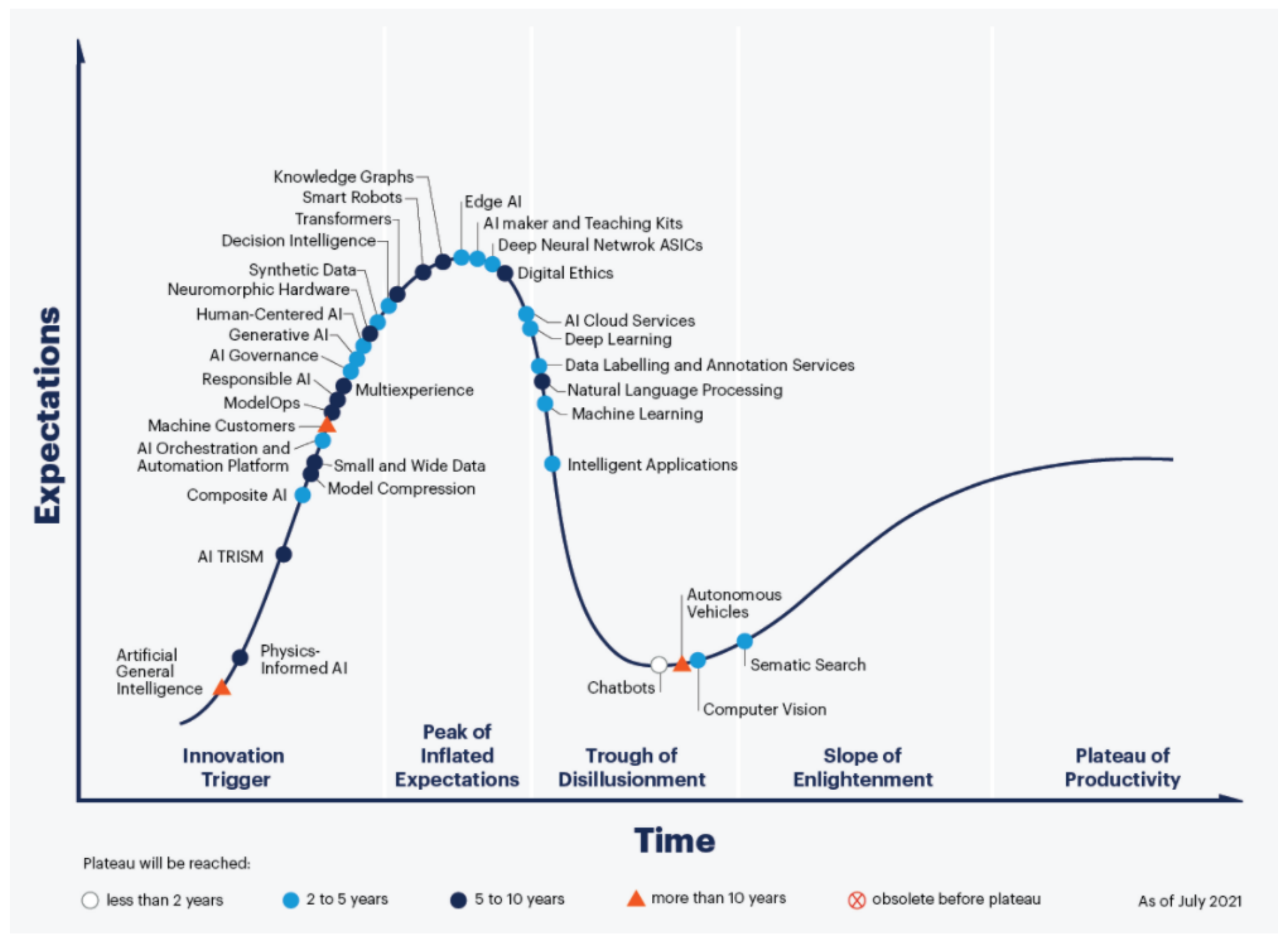
Figure 1 shows Gartner’s hype cycle for artificial intelligence 2021 [27]. The area of responsible artificial intelligence, which includes explainable artificial intelligence, is in the innovation of trigger phase and is expected to reach its plateau of productivity in the next 5 to 10 years.
The input of a machine learning model determines the quality of the model’s output. In other words, the quality and amount of input data are crucial in any machine learning challenge. The same principle works when it comes to the process of explaining a black box model. When using high-quality and realistic data, better patterns can be extracted, and the true state of the system can be obtained. Even though this is a relatively new field of study, there are already a number of papers in the scientific literature that deal with the use of explainable machine learning in the domain of cybersecurity. These papers primarily leverage the KDD Cup 99 [28] and the NSL-KDD datasets [29,30,31,32], with their most important findings being summarized in the continuation of this paragraph. Amarasinghe et al. [29] present a deep neural network anomaly detection framework that provides explanations of detected anomalies. Explanations are provided in the form of a list of features, and their ratings calculated using the layer-wise relevance propagation (LRP) method that indicates the importance of each feature in a specific classification. The research focuses solely on denial of service (DoS) attacks, i.e., distinguishes between benign network traffic and DoS attacks. Mahbooba et al. [28] employ a decision tree and extract if–then rules that are used to discover a set of features that separate benign and malignant traffic (binary classification). The authors calculate feature importance using the entropy measure. Marino et al. [30] present an adversarial approach for generating explanations of data instances that have been incorrectly classified. The approach is used to find the least attribute modifications needed for misclassified data instances to be classified correctly. The size of these modifications is used to determine the most important attributes that explain why the classification is incorrect. Such explanations can be applied to a single data instance or to a group of incorrectly classified data instances, in which case the average attribute modification is applied. The paper employs two approaches to network traffic classification, linear and multilayer perceptron classifiers. The authors of [31] describe a deep neural network for network traffic classification and five algorithms for explaining its results. Shapley additive explanations (SHAP), local interpretable model-agnostic explanations (LIME), contrastive explanation method (CEM), ProtoDash, and Boolean decision rules via column generation (BRCG) are the used explanatory algorithms, and explanations are generated both locally and globally. The paper performs binary classification. Wang et al. [32] explain the results of two classifiers, the one-vs-all classifier, and the multiclass classifier, using the SHAP method. Local explanations attempt to determine why a specific instance is classified in a particular manner, whereas global explanations identify the most important attributes that distinguish individual classes.
Both the KDD Cup 99 dataset and the NSL-KDD dataset have significant flaws—most notably, the obsolescence of attacks in the datasets as well as the synthetic origin of the datasets. In 2017, the Canadian Institute for Cybersecurity released a new dataset—CIC-IDS2017. This dataset contains benign network traffic and a wide range of more contemporary attack scenarios, closely resembling authentic real-world data. This is what currently makes the CIC-IDS2017 a much better choice when building and explaining machine learning models in the cybersecurity domain. Several papers already used the CIC-IDS2017 dataset in the domain of explainable machine learning. Dang [33] uses explainable machine learning models to improve the performance of the intrusion detection systems. The author analyzes the extreme gradient boosting (xgboost) model performance by comprehending feature influence and removing unnecessary features. The author then compares the performance of model post-explainability-based feature selection to that of prior-explainability-based feature selection. According to the author, by forcing explainability, the model becomes more robust, requires less computational power, and achieves better predictive performance. The author performs feature understanding of the model using the partial dependence plot (PDP) and SHAP values and is focused on binary as well as a multiclass classification problem. Szczepanski et al. [34] use a feed forward artificial neural network to classify the network traffic and use surrogate decision trees to find the most likely explanations for a classified sample. Das et al. [35] propose a confident and explainable anomaly detector based on random forest, multilayer perceptron, and support vector machine classifiers. The authors then interpret the predictions using the LIME method. The paper mainly focuses on finding the most influential benign and malign dataset features. Liu et al. [36] propose an interpretable convolutional neural network based on spatial domain attention. The model can discover and locate specific malicious packet fields, which can then be interpreted. To improve the model explainability, Islam et al. [37] incorporate confidentiality, integrity, and availability principles into the model in the form of newly defined features. In more detail, the author implements a feature generalizer component that takes the original features of the CIC-IDS2017 dataset and infuses domain knowledge to produce/re-construct a concise and better interpretable feature set. The authors then compare the advantages or disadvantages of incorporating domain knowledge in the experiment using the evaluator component that, using four different feature configurations, compares the performance of naïve Bayes, artificial neural network, support vector machine, random forest, extra trees, and gradient boosting models. Although Bachl et al. [38] are not focused on the explainability of the machine learning model, they do mention it in one section of their paper. In particular, they show how visualization techniques from explainable machine learning can be used to detect backdoors and problems emerging from the distribution of attack samples in the training dataset. PDP and accumulated local effects (ALE) are used by the authors to find the backdoors and incorrect decisions. Callegari et al. [39] concentrate their attention on an explainable method for classifying internet traffic that can inform practitioners of the results of the classification. More specifically, their suggested method is based on a multi-objective evolutionary fuzzy classifier, which, in their opinion, offers a good trade-off between the resulting classification models’ accuracy and explainability. The experimental results are obtained using the UniBS and UPC datasets.
Taking into account the information gained from the currently published scientific papers, our research is the first to use explainable machine learning to extract information from the CIC-IDS2017 dataset and to critically compare the challenges of the knowledge extraction process while analyzing if–then decision tree rules and while using the SHAP approach. The paper discusses the benefits and drawbacks of if–then decision tree rules and the rules produced by the SHAP method, and it makes recommendations for which approach to use in particular circumstances.
2. Materials and Methods
2.1. Methodology
In many domains, the ability to understand the inner workings of a predictive model is critical. To satisfy this requirement, intrinsically interpretable machine learning models are commonly used.
These models, however, frequently underperform in terms of prediction and classification, making such an approach unsuitable for fields where great precision is necessary. This becomes a common issue in the cybersecurity domain where both interpretability and high precision are usually given top priority.
The goal of this paper is to extract knowledge from the CIC-IDS2017 dataset using the SHAP method, as well as comparing the possibilities of extracting knowledge using the specified method and by analyzing the decision tree rules. The paper discusses which approach is more appropriate in specific situations, as well as the advantages and disadvantages of both approaches. To allow for the direct comparison of the rules extracted with the SHAP method and the decision tree rules, the SHAP method is implemented on a decision tree model. Once we demonstrate that the SHAP is sufficient to obtain a global picture of the model, we can successfully pave the way toward implementing an interpretability layer over any chosen black box model.
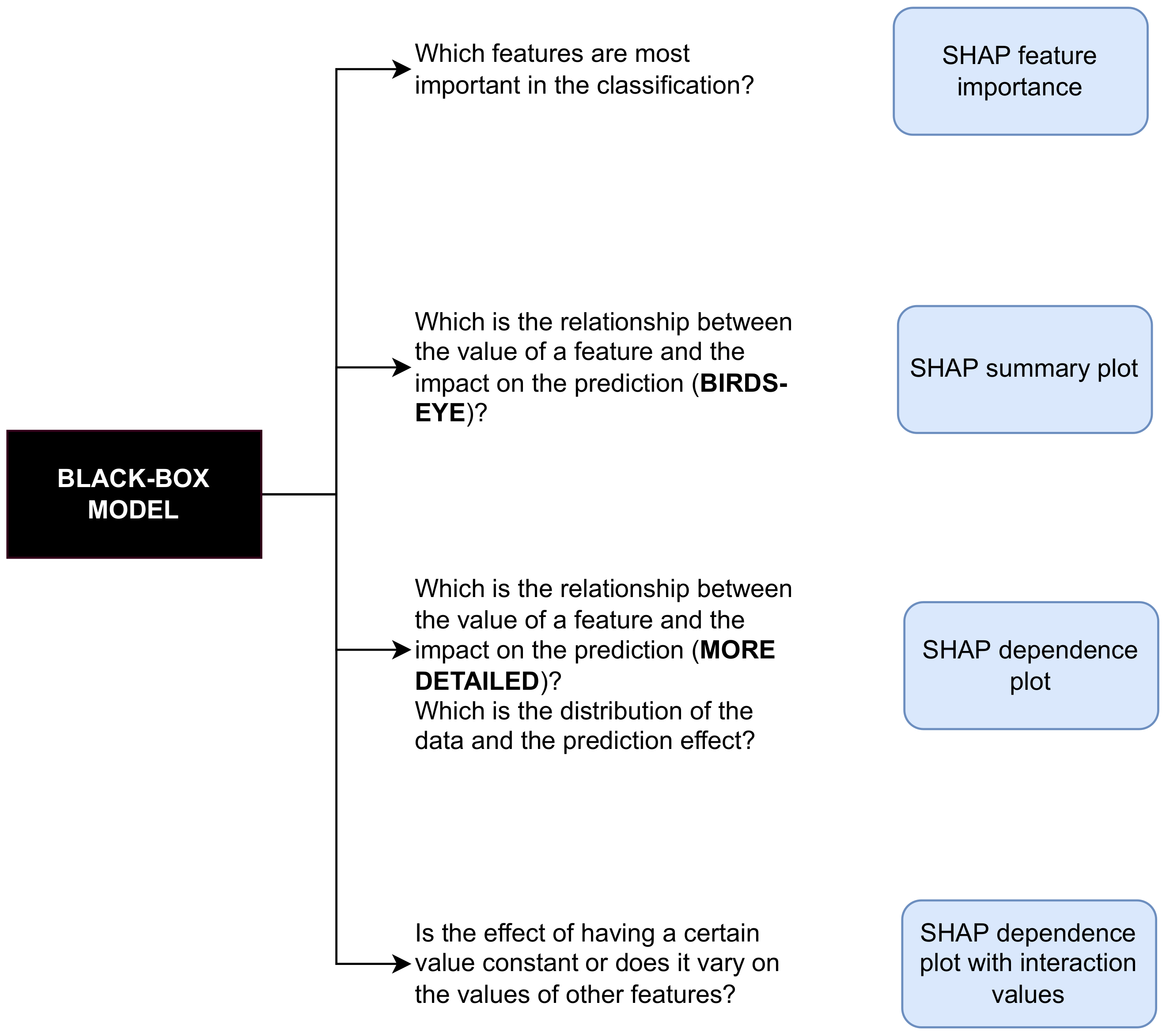
Although SHAP is primarily a local interpretability method, it can also be used to explain machine learning models globally. This paper will showcase the usage of SHAP method for global interpretations. Figure 2 outlines the main questions to be answered in the remainder of this paper, while also emphasizing the type of SHAP plot used to obtain answers to the questions and hopefully serving as a useful general guideline for opening a black box model. Henceforth, the proposed methodology can be used in different domains for opening any type of black box model.
2.2. The CIC-IDS2017 Dataset Description
The CIC-IDS2017 dataset contains data related to benign network traffic and a wide range of contemporary attack scenarios, closely approximating authentic real-world data. This dataset was created by the Canadian Institute of Cybersecurity, the data being taken from a simulation that is considerably closer to how a modern computer network behaves compared to the older popular datasets from this domain, with the attacks being carried out with the help of established online tools and tactics. This dataset was hence chosen as the cornerstone research data for this paper.
The original dataset contains 2,830,743 data instances collected over 5 days and described by 79 features (see Table 1). The process of further data preparation was performed in three main steps: data cleaning, data transformation, and feature selection.
Data cleaning step. Infinity and missing values were removed from the CIC-IDS2017 dataset, which resulted in a dataset reduction of 2867 data instances. Following that, the zero variance features (Bwd PSH Flags, Bwd URG Flags, Fwd Avg Bytes/Bulk, Fwd Avg Packets/Bulk, Fwd Avg Bulk Rate, Bwd Avg Bytes/Bulk, Bwd Avg Packets/Bulk, Bwd Avg Bulk Rate) were eliminated. After this step, the dataset contained 2,827,876 rows and 70 columns.
Data transformation step. The CIC-IDS2017 dataset contains benign traffic and 14 different types of attacks (DoS Hulk, PortScan, DDos, DoS GoldenEye, FTP-Patator, SSH-Patator, DoS slowloris, DoS Slowhttptest, Bot, Web Attack Brute Force, Web Attack XSS, Infiltration, Web Attack Sql Injection, Heartbleed) and is highly imbalanced. The majority benign class has a prevalence of 80.32%, while the minority heartbleed class has a prevalence of 0.00039%. Due to the under-representation of certain types of attacks, this paper conflated some of the classes while removing others altogether. More precisely, DoS Hulk, DoS GoldenEye, DoS slowloris, and DoS Slowhttptest attacks were merged into the DoS class. FTP-Patator and SSH-Patator were merged into the Brute Force class. The benign, and port scan attack classes were held in their original form, and other attack types were removed from the dataset. The final dataset, therefore, contained benign traffic and 4 classes of attacks—DoS attacks, DDoS attacks, brute force attacks, and port scan attacks. This dataset was then divided into a training set and test set (70:30), with random oversampling and random undersampling being performed on the training part of the dataset for the purposes of class balancing.
Feature selection step. This paper uses the SHAP feature importance method. The SHAP feature importance method measures the influence of a feature by comparing the model prediction with and without the feature, and ranks features with larger absolute Shapley values as more important. The method is consistent and accurate [40], and does not overestimate the importance of continuous or high-cardinality categorical variables as native tree-based feature importance methods do. The method chose 12 most important features: Destination Port, Bwd Packet Length Min, Init_Win_bytes_backward, Subflow Fwd Bytes, Packet Length Mean, min_seg_size_forward, Bwd Packets/s, PSH Flag Count, Fwd Header Length.1, Init_Win_bytes_forward, Flow IAT Mean, and Total Length of Fwd Packets.
2.3. Decision Tree
Decision tree is a type of supervised machine learning model that learns simple decision rules inferred from prior data and predicts the class or the value of a target variable. The decision model is built top-down in the form of a tree structure, beginning with the root node and progressing to decision nodes and leaf nodes. The root nodes are important predictors, while the leaf nodes provide the final classification. This paper focuses on CART decision trees. The CART decision tree algorithm builds a binary decision tree by performing a greedy top-down search through the given set of training data. The greedy approach is based on the concept of heuristic problem solving, which involves making the best local choices at each node to reach the approximation of the global optimum. There are several functions to measure the quality of a node split. This paper implements the entropy measure, which is a measure of impurity, disorder, or uncertainty in a given dataset.
One of the greatest advantages of the decision tree model is its simple interpretability—one needs to follow the path that begins at the root node and ends at the tree’s leaf, while AND concatenating the rules of all nodes on the path. It is well known that increasing the tree depth results in better model performance in most cases. When it comes to interpretability, increasing the depth of the decision tree reduces the ability to understand the decision-making rules.
2.4. Interpretable Machine Learning Methods
There are a variety of techniques for delving into the inner workings of models, but they frequently come with a cost of diminished accuracy. Such a price is usually not acceptable in the context of cybersecurity, where even minor errors in attack detection can severely impact system performance and cause massive damage. Therefore, the choice of interpretability methods in the domain of cybersecurity is limited. This paper implements the SHAP method to explain machine learning models used to detect cyber attacks. However, before explaining the SHAP method, it is necessary to define a few essential concepts needed to comprehend this paper. Intrinsic interpretability refers to machine learning methods that are interpretable because of their simple structure. Post-hoc interpretability refers to the use of interpretable methods after model training. Model-specific interpretability methods are those that are restricted to particular model classes. Model-agnostic interpretability methods can be used on any machine learning model and are applied after model training (post-hoc). Local methods explain individual predictions. Global methods explain the entire model behavior.
Finally, because SHAP connects two local model-agnostic methods, LIME, proposed in [1], and Shapley values, proposed in [41], it is important to explain all three methods in more detail.
2.4.1. Shapley Values
Shapley values are a concept borrowed from the literature of cooperative game theory, and they were originally used to fairly attribute a player’s contribution to the end result of a game. An assumption is made that a cooperative game exists in which a set of players works together to achieve some value. Shapley values capture the marginal contribution of each player to the end result. The method can be used to interpret the machine learning prediction by assuming that each feature value of the instance is a player in a game where the prediction is the payout.
Mathematically, the Shapley value is the average contribution of a feature value to the prediction in all feasible coalitions. The Shapley value for feature j is calculated as follows (see Equation (1)):
where
- N = set of all features
- S = a subset of the features used in the model
- = a function that gives a prediction for any subset of features
Simply put, the Shapley value for a feature is calculated as follows:
- Create the set of all possible feature combinations S (called coalitions).
- Calculate the average model prediction.
- For each coalition, calculate the difference between the model’s prediction without feature j and the average prediction.
- For each coalition, calculate the difference between the model’s prediction with feature j and the average prediction.
- For each coalition, calculate how much the feature j changed the model’s prediction from the average (the difference between the values calculated in steps 4 and 3)—this is the marginal contribution of a feature j.
- The Shapley value is the average of all the values calculated in step 5 (i.e., the average of features’ j marginal contributions).
It is important to note that when constructing all possible coalitions, the input features that are not observed in that specific coalition are not removed (because this changes the input dimension), but are instead replaced with random samples from the training dataset. The Shapley value calculation is very time consuming. For a set of n features, there are coalitions (subsets) that should be analyzed in order to compute the Shapley values.
2.4.2. Local Interpretable Model-Agnostic Explanations, LIME
LIME is a concrete implementation of local surrogate models. Surrogate models are intrinsic interpretable models trained to approximate the underlying black box model’s predictions. The conclusions about the black box models can then be drawn by interpreting the surrogate model. Local surrogate models, such as LIME, are focused on explaining individual predictions.
Mathematically, LIME is described as follows (see Equation (2)):
where
- g = the explanation model for instance x (e.g., linear regression model).
- G = the family of all possible explanations (e.g., all possible linear regression models).
- L = the loss function (e.g., mean squared error) used to measure how close the explanation is to the prediction of the original black box model.
- f = the original black box model.
- = the proximity measure used to define how large the neighborhood around instance x is that we consider for the explanation.
- (g) = the model complexity.
Simply put, LIME investigates what happens to predictions when variations of the data are fed into a machine learning model. LIME creates a new dataset that contains perturbed samples as well as the black box model’s predictions for those samples. LIME then trains an intrinsic interpretable machine learning model on this newly created dataset. The intrinsic interpretable machine learning model that best approximates the black box model is found by calculating the Equation (2). The trained intrinsic interpretable machine learning model can then be used to explain the black box model predictions. To summarize, the goal of local surrogate models is to replicate the underlying black box model’s predictions as closely as is feasible while being interpretable.
2.4.3. Shapley Additive Explanations, SHAP
SHAP is a model-agnostic machine learning interpretability method proposed by the authors Lundberg and Lee [3], and it combines Shapley values and the LIME method. The main advantage of SHAP is that, inspired by local surrogate models, it allows for a more computationally efficient estimation of Shapley values when used in machine learning. In more detail, SHAP explains individual instance predictions by computing the contributions of each feature to the prediction—each feature can contribute positively (SHAP value is greater than zero) to the prediction, negatively (SHAP value is less than zero) to the prediction, or can have no impact on the prediction (SHAP value is zero). Although SHAP is basically a local interpretable method, it can also be used as a global method. In SHAP, the Shapley value explanation is represented as a linear model.
Mathematically, SHAP values can be calculated as follows (see Equation (3)):
where
g = the explanation model.
= the coalition vector. An entry of 1 means that the corresponding feature value is “present” and 0 that it is “absent”.
M = the maximum coalition size.
= the feature attribution for a feature j for instance x (the approximated Shapley values).
Simply put, the goal of SHAP is to approximate Shapley values in order to reduce the complexity of calculating them. SHAP takes a data subset and fits a linear regression model to it (similar to LIME). The variables in this linear regression model are zeros and ones that represent whether a feature is present or absent, and the output value is the prediction. Following model training, the linear model’s coefficients can be interpreted as Shapley value approximations. There are several methods by which this can be achieved, Kernel SHAP, Tree SHAP, and Deep SHAP. Note: The term SHAP refers to the Kernel SHAP. This paper implements Tree SHAP, an efficient Shapley value estimation approach used for tree-based models. Tree SHAP was introduced by [40] as a fast, model-specific alternative to Kernel SHAP, but it has proven to produce unintuitive feature attributions. Instead of the marginal expectation, the Tree SHAP method uses the conditional expectation instead of in Equation (1). When compared to Kernel SHAP, Tree SHAP reduces the computational complexity from to . The parameter T is the number of trees, L is the maximum number of leaves in any tree and D is the maximal depth of any tree. For more detail about the algorithm for estimating the conditional expectation , the Tree SHAP algorithm and the complexity, see [40].
3. Results
This paper implements a multi-class decision tree classifier. Class 0 represents the benign network traffic, class 1 DoS attacks, class 2 DDoS attacks, class 3 port scan attacks, and finally class 4 brute force attacks. The confusion matrix demonstrates the performance of the decision tree classifier after hyperparameter optimization.
3.1. SHAP Feature Importance
Figure 3 shows the SHAP feature importance plot for the implemented decision tree. The global importance of each feature is taken to be the mean absolute SHAP value for that feature over all given samples. Features with larger absolute SHAP values are globally more important. In addition to the feature’s global importance, the figure also shows the relative relevance of each feature for each class (see the length of the bar for each class. Each class has a different bar color).
The Destination Port, Bwd Packet Length Min, and Init_Win_bytes_backward features are the three globally most important features in the classification of the network traffic. Although the Destination Port feature is not among the top five features in the classification of port scan attacks, it is one of the most important features in the classification of benign traffic, DoS attacks, DDoS attacks, and brute force attacks. In more detail, the Destination Port feature is the most important feature in the classification of benign traffic and brute force attacks, and it is the second most important feature in the classification of DoS and DDoS attacks. Therefore, the rest of this paper will concentrate on a more in-depth examination of the Destination Port feature.
3.2. SHAP Summary Plot
Although the SHAP feature importance plot is very useful, it contains no information other than the feature importance. To conduct a more detailed analysis, SHAP summary plots for each class must be examined (see Figure 4). The SHAP summary plot provides a thorough explanation of a model that incorporates feature importance (note that the features are sorted by importance for each class) and feature effect. Each instance has a single dot on each row. The dot’s x position represents the feature’s influence on the model’s prediction for the instance, and the dot’s color represents the feature’s value for the instance. To demonstrate density, dots that do not fit on the row pile up. The x-axis is expressed in log odds.
By examining the Destination Port feature on Figure 4a, one can conclude that benign traffic is distinguished by high values of that feature. It is worth noting that data instances with low Destination Port values might also be categorized as benign traffic. In this case, additional analyses are required since low values of the Destination Port feature are more typical for another class, which will be explained in the rest of the paper (see dependence plot section). When analyzing Figure 4b, one can notice that low values of the Destination Port feature are highly indicative of a DoS attack. What can be argued with even greater certainty when analyzing Figure 4b is that when the Destination Port feature takes on high values, it is most often not a DoS attack.
The analysis of the Destination Port feature of the summary plots for the DDoS class (see Figure 4c) and the port scan class (see Figure 4d) yield similar conclusions. When the value of the Destination Port feature is low, we are less likely to claim that it is a DDoS attack instead of a DoS attack (notice the amount of blue on the graph’s left side in Figure 4c). By examining the Destination Port feature in Figure 4e, it is important to notice that low values of the Destination Port feature are also indicative of brute force attacks, but further investigation is required since low values of this attribute are also indicative of another class. It is important to note that although we only covered the Destination Port feature in the study, other features are also displayed in the plots to ensure thorough analysis.
Some of the conclusions we reached by analyzing the SHAP summary plots can also be reached by examining the decision tree’s if–then rules. In particular, the decision tree can be used to determine which spectrum of values of a given feature is typical for a given class. In fact, the decision tree can provide a much more detailed understanding of the above. Using the if–then rules, it is possible to create more granular feature intervals while the SHAP summary plot “cuts” the samples into two intervals (low, and high feature values). Regardless of the foregoing, the analysis of if–then rules is both demanding and exhaustive if the tree depth is large. There are numerous if–then rules, and the same features and separation criteria can be repeated multiple times at various depths in the decision tree. What can be seen in the SHAP summary plots but not in the decision tree’s if–then rules is how much each feature influences the prediction.
3.3. SHAP Dependence Plot without Interaction Feature
In order to obtain a more detailed insight into the relationship between a specific port and its impact on predictions, it is important to analyze the dependence plots. SHAP dependence plots depict the impact of a single feature on the entire dataset. They plot the value of a feature vs. its SHAP value across many samples. The vertical dispersion of SHAP values at a single feature value is driven by interaction effects, and another feature is chosen for coloring to highlight possible interactions. SHAP dependence plots (without interaction features) for the Destination Port feature are shown on Figure 5. The figure only displays the ports from the interval [15, 85]. The three most popular ports in the data set, ports 21, 22, and 80, are intended to be included. The SHAP values of the Destination Port feature for the values of features 21 and 22 for the benign class are extremely negative (see Figure 5a). This suggests that these destination port feature values are more likely to represent attacks than benign network activity. The figure also demonstrates that a very small proportion of data occurrences can nevertheless be benign (SHAP values are positive). The absolute value of these SHAP values is incredibly low, and only a tiny fraction of the data instances have such SHAP values (see the shade of blue). Without further analysis, it is impossible to distinguish between benign traffic and an attack when the port takes the value 80 (see Figure 5a)—notice that there are both positive and negative SHAP values, and their absolute value is low. Similar to the benign class, if the Destination Port feature takes the values 21 and 22, it is most likely not a DoS attack (see Figure 5b), nor a DDoS attack (see Figure 5c). When the port is 80, the situation is exactly the opposite. In this case, there is a high likelihood of a DoS or DDoS attack. If the port scan class is analyzed, one can once again conclude that the Destination Port attribute does not carry much information (see Figure 5d). SHAP values oscillate around zero, and when the Destination Port feature takes the value 21 or 22, it is impossible, without additional analysis, to determine whether it is a port scan class or another class. The port value of 80 is not typically associated with a port scan attack, though it is present in a small proportion of network instances that are classified as such. If the Destination Port attribute takes the values 21 and 22, there is a high probability that it is a brute force attack (see Figure 5e). Namely, the SHAP values, in this case, are extremely positive. Port 80, on the other hand, is not typical for brute force attacks.
Conclusions drawn from analyzing SHAP dependence plots without interaction feature cannot be drawn from analyzing decision tree if–then rules. Specifically, the decision tree does not indicate how much the value of a particular feature contributes to the prediction. As previously stated, the if–then rule can be used to determine which value spectrum of a specific feature is characteristic of a specific class. However, analyzing a concrete value of a discrete feature is not always possible from the if–then rules of a decision tree. Note that it is possible for a decision tree to give rules for a specific value of a discrete feature. However, even if it does, it is quite challenging to locate and analyze each of these rules in a lengthy list of rules.
3.4. SHAP Dependence Plot with Interaction Feature
Based on the previous analysis, it was concluded that when the port value is 80, the traffic may or may not be benign (see Figure 5a). In this case, further investigation and observation of the interaction feature are required. The best interaction feature in this particular case is the PSH Flag Count, a binary feature that takes the values 0 and 1. Figure 6 shows a SHAP dependence plot of the Destination Port feature combined with the PSH Flag Count interaction feature for the benign class. If a data instance takes the value of the Destination Port feature 80, and if, at the same time, the PSH Flag Count feature takes the value 1, it is most likely benign network traffic. Otherwise, it is most likely some kind of attack. A similar analysis can be performed for the port scan class. In the case where the Destination Port attribute takes the values 21 or 22, it may or may not be a port scan attack (see Figure 5d). The best interaction feature in this case is the Fwd Header Length.1 feature (see Figure 7). High values of this feature indicate that it is not an infiltration attack. Although there are data instances with a low value of the Fwd Header Length.1 feature that belong to another class, it is highly likely a port scan attack if the feature takes low values.
Finally, it is necessary to analyze what distinguishes different classes if both (or more) are characterized by the same values of a particular feature.
Ports 21 and 22 were previously identified as being associated with port scan and brute force attacks. Finding an interaction feature that distinguishes these two classes is required. The Fwd Header Length.1 feature is the best interaction feature in this case (see Figure 8). High values of the Fwd Header Length.1 feature are not typical of port scan attacks (see Figure 8a), but rather of brute force attacks (see Figure 8b).
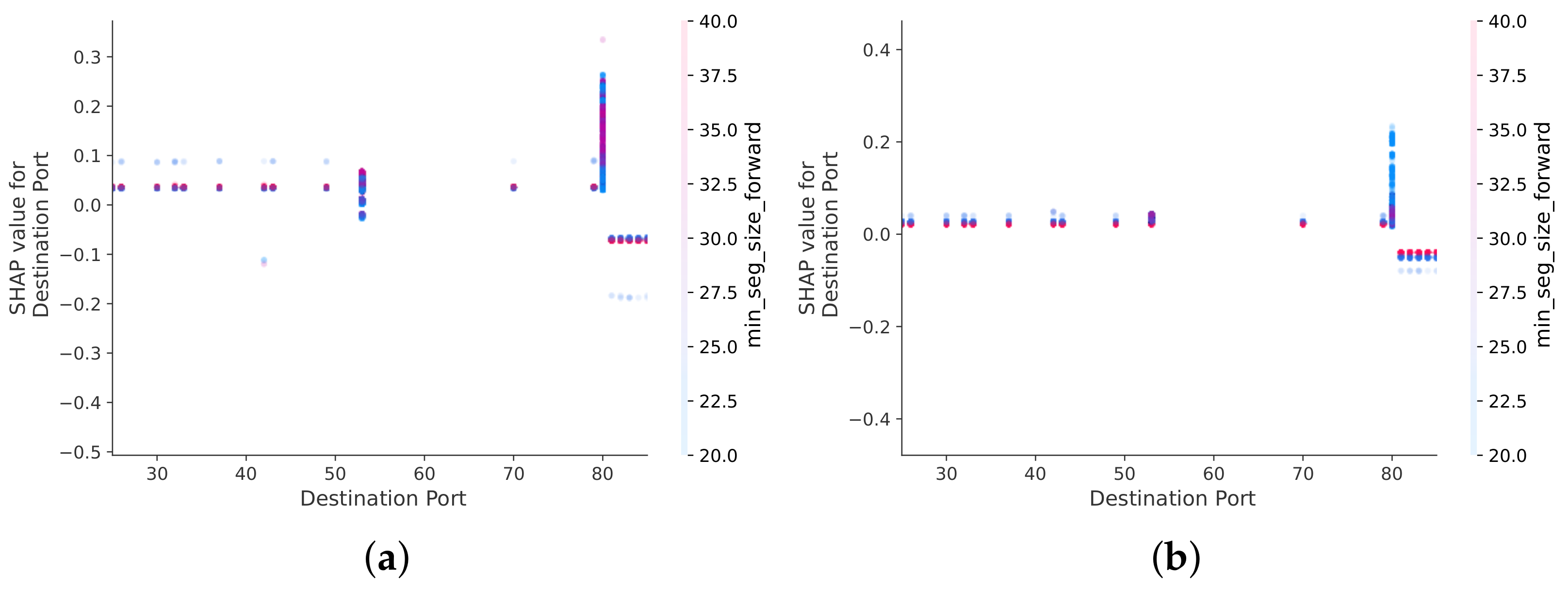
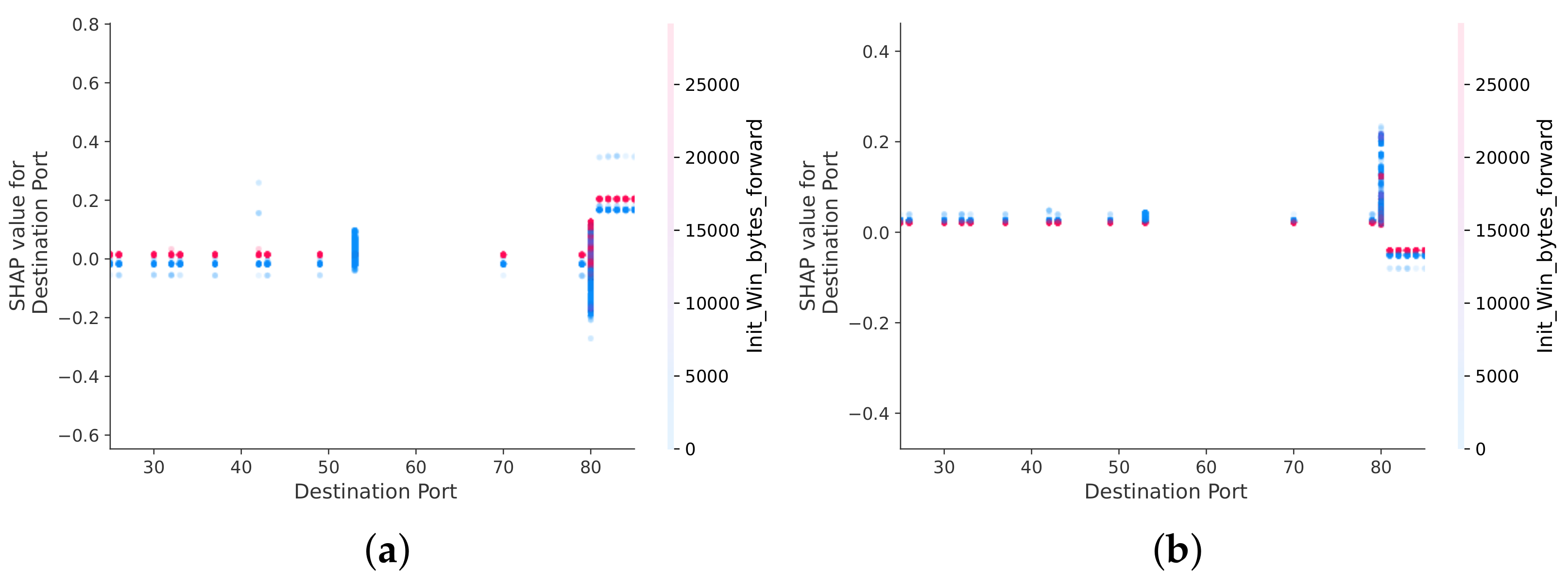
A similar analysis can be carried out for port 80. Port 80, in particular, is associated with benign traffic, as well as DoS and DDoS attacks. The min seg size forward interaction feature is the most effective at distinguishing between DoS and DDoS attacks (see Figure 9). If the value of the min seg size forward feature is high, it is most likely a DoS attack (see Figure 9a), and if it is low, it is most likely a DDoS attack (see Figure 9b). If the port value is 80, the Flow IAT Mean feature best separates benign traffic and DoS attacks (see Figure 10). High values of the Flow IAT mean feature are characteristic of DoS attacks, while low values are characteristic of benign traffic. Finally, the best interaction feature for distinguishing DDoS and benign classes in case the port takes the value 80 is the feature Init_Win_bytes_forward (see Figure 11). High values of the Init_Win_bytes_forward feature characterize benign traffic (see Figure 11a), whereas low values of the Init_Win_bytes_forward feature characterize DDoS attacks (see Figure 11b).
It is important to note that the SHAP method can identify more interaction features. Due to the length of the paper, the paper shows only a few.
As previously stated in the decision tree’s if–then rules, it is not possible to determine how much each feature value influences the prediction. The if–then rules can be used to identify feature interactions. Features that interact with each other are on the same path in the tree and are part of the same rule. The process is, however, very time consuming. If the feature takes on discrete values, that analysis is not always possible. The reason, as before, is the impossibility of analyzing separate values of a discrete variable in the if–then rules of a decision tree.
4. Discussion
Achieving satisfactory levels of transparency is a growing problem as machine learning models become more complex, considerably hindering the deployment of black box intelligent systems in high-risk domains, such as the cybersecurity domain. A significant portion of the scientific literature in the field of cybersecurity is still mostly devoted to enhancing model performance, and the semantic gap in such models continues to pose a significant challenge. This paper focuses on two main goals: first, to successfully extract knowledge from a cybersecurity domain dataset, and second, to critically compare the difficulties encountered during knowledge extraction when evaluating if–then decision tree rules versus using the SHAP method.
The following conclusions can be drawn from the results of knowledge extraction methods that should be generally applicable to the cybersecurity domain. First and foremost, the Destination port feature turns out to be the most important feature globally when it comes to the classification of the network traffic. Furthermore, the Destination port feature is the most important feature in the classification of benign traffic and brute force traffic, and is the second most important feature in the classification of DoS and DDoS attacks. Ports 21 and 22 are identified as being closely associated with port scan and brute force attacks. In this particular case, the Fwd Header Length.1 feature best distinguishes between these two classes. High Fwd Header Length.1 values are more common in brute force attacks than in port scan attacks. Port 80 is associated with benign traffic, as well as DoS and DDoS attacks. In this case, the min seg size forward interaction feature is most effective at distinguishing between DoS and DDoS attacks, the Flow IAT Mean feature best separates benign traffic and DoS attacks, and the Init Win bytes forward feature is the best interaction feature for distinguishing DDoS and benign classes. More precisely, in scenarios involving port 80, the high value of the min seg size forward feature indicates a high probability of a DoS attack, while a low value means the attack is most likely DDoS. In the same vein, high values of the Flow IAT mean feature, again in the case when the destination port takes the value 80, are indicative of DoS attacks, whereas low values are indicative of benign traffic. Finally, high Init Win bytes forward values in the combination with the port value 80 characterize benign traffic, whereas low Init Win bytes forward values characterize DDoS attacks.
If–then decision tree rules provide a very deep understanding of how the classifier functions, but as the depth of the tree increases, the task of examining the rules becomes increasingly challenging. Furthermore, if–then rules cannot be used to determine how a feature affects a prediction, nor to analyze the influence of a discrete feature’s concrete value. As opposed to if–then decision tree rules, SHAP offers a decent overall view of a model despite being less comprehensive. In order to gain a deeper understanding of the model using the SHAP method, it is required to create numerous plots. This paper highlights the precise steps for approaching the black box model opening process using the SHAP method (Figure 2). It is important to notice that the level of detail that may be achieved by if–then rules in a decision tree is still not attainable, even with additional plot drawing. However, this is sufficient to gain an understanding of what is happening behind the curtain, which is the goal of machine learning explainability.
Author Contributions
Conceptualization, A.Š. and A.K.; methodology, A.Š. and A.K; software, A.Š.; validation, A.Š. and A.K.; formal analysis, A.Š.; investigation, A.Š.; resources, A.Š.; data curation, A.Š.; writing—original draft preparation, A.Š.; writing—review and editing, A.Š., A.K., D.P. and M.V.; visualization, A.Š.; supervision, D.P. and M.V.; project administration, D.P.; funding acquisition, D.P. All authors have read and agreed to the published version of the manuscript.
Funding
This research has been supported under Competitiveness and Cohesion Operational Program from the European Regional and Development Fund, as part of the Artificial intelligence system for autonomous monitoring and management of cloud environment security-project no.KK.01.2.1.02.0161 (AI DEFENDER).
Institutional Review Board Statement
Not applicable.
Informed Consent Statement
Not applicable.
Data Availability Statement
The data used in this research can be found at: https://www.unb.ca/cic/datasets/ids-2017.html (accessed on 13 February 2022).
Conflicts of Interest
The authors declare no conflict of interest.
References
- Ribeiro, M.T.; Singh, S.; Guestrin, C. “Why should i trust you?” Explaining the predictions of any classifier. In Proceedings of the 22nd ACM SIGKDD International Conference on Knowledge Discovery and Data Mining, San Francisco, CA, USA, 13–17 August 2016; pp. 1135–1144. [Google Scholar]
- Friedman, J.H. Greedy function approximation: A gradient boosting machine. Ann. Stat. 2001, 29, 1189–1232. [Google Scholar] [CrossRef]
- Lundberg, S.M.; Lee, S.I. A unified approach to interpreting model predictions. Adv. Neural Inf. Process. Syst. 2017, 30, 4768–4777. [Google Scholar]
- Ribeiro, M.T.; Singh, S.; Guestrin, C. Anchors: High-precision model-agnostic explanations. In Proceedings of the AAAI Conference on Artificial Intelligence, New Orleans, LA, USA, 2–7 February 2018; Volume 32. [Google Scholar]
- Wachter, S.; Mittelstadt, B.; Russell, C. Counterfactual explanations without opening the black box: Automated decisions and the GDPR. Harv. JL Tech. 2017, 31, 841. [Google Scholar] [CrossRef]
- Zeiler, M.D.; Fergus, R. Visualizing and understanding convolutional networks. In Proceedings of the European Conference on Computer Vision, Glasgow, UK, 23–28 August 2014; Springer: Berlin/Heidelberg, Germany, 2014; pp. 818–833. [Google Scholar]
- Zhou, B.; Khosla, A.; Lapedriza, A.; Oliva, A.; Torralba, A. Learning deep features for discriminative localization. In Proceedings of the IEEE Conference on Computer Vision and Pattern Recognition, Las Vegas, NV, USA, 27–30 June 2016; pp. 2921–2929. [Google Scholar]
- Linardatos, P.; Papastefanopoulos, V.; Kotsiantis, S. Explainable ai: A review of machine learning interpretability methods. Entropy 2020, 23, 18. [Google Scholar] [CrossRef]
- Cherif, I.L.; Kortebi, A. On using extreme gradient boosting (XGBoost) machine learning algorithm for home network traffic classification. In Proceedings of the 2019 IEEE Wireless Days (WD), Manchester, UK, 24–26 April 2019; pp. 1–6. [Google Scholar]
- Mohammed, A.R.; Mohammed, S.A.; Shirmohammadi, S. Machine learning and deep learning based traffic classification and prediction in software defined networking. In Proceedings of the 2019 IEEE International Symposium on Measurements & Networking (M&N), Catania, Italy, 8–10 July 2019; pp. 1–6. [Google Scholar]
- Salman, O.; Elhajj, I.H.; Kayssi, A.; Chehab, A. A review on machine learning–based approaches for Internet traffic classification. Ann. Telecommun. 2020, 75, 673–710. [Google Scholar] [CrossRef]
- Sun, G.; Liang, L.; Chen, T.; Xiao, F.; Lang, F. Network traffic classification based on transfer learning. Comput. Electr. Eng. 2018, 69, 920–927. [Google Scholar] [CrossRef]
- D’Angelo, G.; Palmieri, F. Network traffic classification using deep convolutional recurrent autoencoder neural networks for spatial–temporal features extraction. J. Netw. Comput. Appl. 2021, 173, 102890. [Google Scholar] [CrossRef]
- Iliyasu, A.S.; Deng, H. Semi-supervised encrypted traffic classification with deep convolutional generative adversarial networks. IEEE Access 2019, 8, 118–126. [Google Scholar] [CrossRef]
- Lim, H.K.; Kim, J.B.; Heo, J.S.; Kim, K.; Hong, Y.G.; Han, Y.H. Packet-based network traffic classification using deep learning. In Proceedings of the 2019 IEEE International Conference on Artificial Intelligence in Information and Communication (ICAIIC), Okinawa, Japan, 11–13 February 2019; pp. 46–51. [Google Scholar]
- Li, R.; Xiao, X.; Ni, S.; Zheng, H.; Xia, S. Byte segment neural network for network traffic classification. In Proceedings of the 2018 IEEE/ACM 26th International Symposium on Quality of Service (IWQoS), Banff, AB, Canada, 4–6 June 2018; pp. 1–10. [Google Scholar]
- Carvalho, D.V.; Pereira, E.M.; Cardoso, J.S. Machine learning interpretability: A survey on methods and metrics. Electronics 2019, 8, 832. [Google Scholar] [CrossRef]
- Richardson, A.; Rosenfeld, A. A survey of interpretability and explainability in human-agent systems. In Proceedings of the XAI Workshop on Explainable Artificial Intelligence, Stockholm, Sweden, 14–15 July 2018; 2019; 33, pp. 637–705. [Google Scholar]
- Tjoa, E.; Guan, C. A survey on explainable artificial intelligence (xai): Toward medical xai. IEEE Trans. Neural Netw. Learn. Syst. 2020, 32, 4793–4813. [Google Scholar] [CrossRef] [PubMed]
- Hansen, L.K.; Rieger, L. Interpretability in intelligent systems–A new concept. In Explainable AI: Interpreting, Explaining and Visualizing Deep Learning; Springer: Berlin/Heidelberg, Germany, 2019; pp. 41–49. [Google Scholar]
- Rudin, C. Stop explaining black box machine learning models for high stakes decisions and use interpretable models instead. Nat. Mach. Intell. 2019, 1, 206–215. [Google Scholar] [CrossRef] [Green Version]
- Lipton, Z.C. The mythos of model interpretability: In machine learning, the concept of interpretability is both important and slippery. Queue 2018, 16, 31–57. [Google Scholar] [CrossRef]
- Arrieta, A.B.; Díaz-Rodríguez, N.; Del Ser, J.; Bennetot, A.; Tabik, S.; Barbado, A.; García, S.; Gil-López, S.; Molina, D.; Benjamins, R.; et al. Explainable Artificial Intelligence (XAI): Concepts, taxonomies, opportunities and challenges toward responsible AI. Inf. Fusion 2020, 58, 82–115. [Google Scholar] [CrossRef]
- Roscher, R.; Bohn, B.; Duarte, M.F.; Garcke, J. Explainable machine learning for scientific insights and discoveries. IEEE Access 2020, 8, 42200–42216. [Google Scholar] [CrossRef]
- Yuan, H.; Yu, H.; Gui, S.; Ji, S. Explainability in graph neural networks: A taxonomic survey. arXiv 2020, arXiv:2012.15445. [Google Scholar]
- Montavon, G.; Samek, W.; Müller, K.R. Methods for interpreting and understanding deep neural networks. Digit. Signal Process. 2018, 73, 1–15. [Google Scholar] [CrossRef]
- Gartner Identifies Four Trends Driving Near-Term Artificial Intelligence Innovation. Available online: https://www.gartner.com/en/newsroom/press-releases/2021-09-07-gartner-identifies-four-trends-driving-near-term-artificial-intelligence-innovation (accessed on 7 May 2022).
- Mahbooba, B.; Timilsina, M.; Sahal, R.; Serrano, M. Explainable artificial intelligence (xai) to enhance trust management in intrusion detection systems using decision tree model. Complexity 2021, 2021, 6634811. [Google Scholar] [CrossRef]
- Amarasinghe, K.; Kenney, K.; Manic, M. Toward explainable deep neural network based anomaly detection. In Proceedings of the 2018 IEEE 11th International Conference on Human System Interaction (HSI), Gdansk, Poland, 4–6 July 2018; pp. 311–317. [Google Scholar]
- Marino, D.L.; Wickramasinghe, C.S.; Manic, M. An adversarial approach for explainable ai in intrusion detection systems. In Proceedings of the IECON 2018-44th Annual Conference of the IEEE Industrial Electronics Society, Washington, DC, USA, 21–23 October 2018; pp. 3237–3243. [Google Scholar]
- Mane, S.; Rao, D. Explaining network intrusion detection system using explainable AI framework. arXiv 2021, arXiv:2103.07110. [Google Scholar]
- Wang, M.; Zheng, K.; Yang, Y.; Wang, X. An explainable machine learning framework for intrusion detection systems. IEEE Access 2020, 8, 73127–73141. [Google Scholar] [CrossRef]
- Dang, Q.V. Improving the performance of the intrusion detection systems by the machine learning explainability. Int. J. Web Inf. Syst. 2021, 17, 537–555. [Google Scholar] [CrossRef]
- Szczepanski, M.; Komisarek, M.; Pawlicki, M.; Kozik, R.; Choraś, M. The Proposition of Balanced and Explainable Surrogate Method for Network Intrusion Detection in Streamed Real Difficult Data. In Proceedings of the International Conference on Computational Collective Intelligence, Bristol, UK, 5–7 September 2018; Springer: Berlin/Heidelberg, Germany, 2021; pp. 241–252. [Google Scholar]
- Das, T.; Shukla, R.M.; Sengupta, S. The Devil is in the Details: Confident & Explainable Anomaly Detector for Software-Defined Networks. In Proceedings of the 2021 IEEE 20th International Symposium on Network Computing and Applications (NCA), Boston, MA, USA, 23–26 November 2021; pp. 1–5. [Google Scholar]
- Liu, H.; Lang, B.; Chen, S.; Yuan, M. Interpretable deep learning method for attack detection based on spatial domain attention. In Proceedings of the 2021 IEEE Symposium on Computers and Communications (ISCC), Athens, Greece, 5–8 September 2021; pp. 1–6. [Google Scholar]
- Islam, S.R.; Eberle, W.; Ghafoor, S.K.; Siraj, A.; Rogers, M. Domain knowledge aided explainable artificial intelligence for intrusion detection and response. arXiv 2019, arXiv:1911.09853. [Google Scholar]
- Bachl, M.; Hartl, A.; Fabini, J.; Zseby, T. Walling up backdoors in intrusion detection systems. In Proceedings of the 3rd ACM CoNEXT Workshop on Big Data, Machine Learning and Artificial Intelligence for Data Communication Networks, Orlando, FL, USA, 9 December 2019; pp. 8–13. [Google Scholar]
- Callegari, C.; Ducange, P.; Fazzolari, M.; Vecchio, M. Explainable internet traffic classification. Appl. Sci. 2021, 11, 4697. [Google Scholar] [CrossRef]
- Lundberg, S.M.; Erion, G.G.; Lee, S.I. Consistent individualized feature attribution for tree ensembles. arXiv 2018, arXiv:1802.03888. [Google Scholar]
- Shapley, L.S. A Value for N-Person Games; RAND Corporation: Santa Monica, CA, USA, 1952. [Google Scholar] [CrossRef]
Figure 1.
Gartner hype cycle.

Figure 2.
Guidelines for opening the black box model using the SHAP method.

Figure 3.
SHAP feature importance plot.

Figure 4.
Summary plots. (a) Benign; (b) Dos; (c) DDos; (d) Port scan; (e) Brute force.

Figure 5.
Dependence plots. (a) Benign; (b) DoS; (c) DDoS; (d) Port scan; (e) Brute force.

Figure 6.
PSH Flag Count/Destination Port interaction for benign network.

Figure 7.
Fwd Header Length.1/Destination Port interaction for port scan attacks.

Figure 8.
Fwd Header Length.1/Destination Port interaction plots. (a) Fwd Header Length.1/ Destination Port interaction for port scan attacks; (b) Fwd Header Length.1/Destination Port interaction for brute force attacks.
Figure 8.
Fwd Header Length.1/Destination Port interaction plots. (a) Fwd Header Length.1/ Destination Port interaction for port scan attacks; (b) Fwd Header Length.1/Destination Port interaction for brute force attacks.

Figure 9.
Min seg size forward/Destination Port interaction plots. (a) Min seg size forward/ Destination Port interaction for DoS attacks; (b) Min seg size forward/Destination Port interaction for DDoS attacks.
Figure 9.
Min seg size forward/Destination Port interaction plots. (a) Min seg size forward/ Destination Port interaction for DoS attacks; (b) Min seg size forward/Destination Port interaction for DDoS attacks.

Figure 10.
Flow IAT Mean/Destination Port interaction plots. (a) Flow IAT Mean/Destination Port interaction for benign traffic; (b) Flow IAT Mean/Destination Port interaction for DoS attacks.
Figure 10.
Flow IAT Mean/Destination Port interaction plots. (a) Flow IAT Mean/Destination Port interaction for benign traffic; (b) Flow IAT Mean/Destination Port interaction for DoS attacks.

Figure 11.
Init Win bytes forward/Destination Port interaction plots. (a) Init Win bytes forward/ Destination Port interaction for benign traffic; (b) Init Win bytes forward/Destination Port interaction for DDoS attacks.
Figure 11.
Init Win bytes forward/Destination Port interaction plots. (a) Init Win bytes forward/ Destination Port interaction for benign traffic; (b) Init Win bytes forward/Destination Port interaction for DDoS attacks.


Table 1.
Dataset features.
| No. | Feature | No. | Feature | No. | Feature |
|---|---|---|---|---|---|
| 1 | Destination Port | 28 | Bwd IAT Std | 55 | Avg Bwd Segment Size |
| 2 | Flow Duration | 29 | Bwd IAT Max | 56 | Fwd Header Length.1 |
| 3 | Total Fwd Packets | 30 | Bwd IAT Min | 57 | Fwd Avg Bytes/Bulk |
| 4 | Total Backward Packets | 31 | Fwd PSH Flags | 58 | Fwd Avg Packets/Bulk |
| 5 | Total Length of Fwd Packets | 32 | Bwd PSH Flags | 59 | Fwd Avg Bulk Rate |
| 6 | Total Length of Bwd Packets | 33 | Fwd URG Flags | 60 | Bwd Avg Bytes/Bulk |
| 7 | Fwd Packet Length Max | 34 | Bwd URG Flags | 61 | Bwd Avg Packets/Bulk |
| 8 | Fwd Packet Length Min | 35 | Fwd Header Length | 62 | Bwd Avg Bulk Rate |
| 9 | Fwd Packet Length Mean | 36 | Bwd Header Length | 63 | Subflow Fwd Packets |
| 10 | Fwd Packet Length Std | 37 | Fwd Packets/s | 64 | Subflow Fwd Bytes |
| 11 | Bwd Packet Length Max | 38 | Bwd Packets/s | 65 | Subflow Bwd Packets |
| 12 | Bwd Packet Length Min | 39 | Min Packet Length | 66 | Subflow Bwd Bytes |
| 13 | Bwd Packet Length Mean | 40 | Max Packet Length | 67 | Init_Win_bytes_forward |
| 14 | Bwd Packet Length Std | 41 | Packet Length Mean | 68 | Init_Win_bytes_backward |
| 15 | Flow Bytes/s | 42 | Packet Length Std | 69 | act_data_pkt_fwd |
| 16 | Flow Packets/s | 43 | Packet Length Variance | 70 | min_seg_size_forward |
| 17 | Flow IAT Mean | 44 | FIN Flag Count | 71 | Active Mean |
| 18 | Flow IAT Std | 45 | SYN Flag Count | 72 | Active Std |
| 19 | Flow IAT Max | 46 | RST Flag Count | 73 | Active Max |
| 20 | Flow IAT Min | 47 | PSH Flag Count | 74 | Active Min |
| 21 | Fwd IAT Total | 48 | ACK Flag Count | 75 | Idle Mean |
| 22 | Fwd IAT Mean | 49 | URG Flag Count | 76 | Idle Std |
| 23 | Fwd IAT Std | 50 | CWE Flag Count | 77 | Idle Max |
| 24 | Fwd IAT Max | 51 | ECE Flag Count | 78 | Idle Min |
| 25 | Fwd IAT Min | 52 | Down/Up Ratio | 79 | Label |
| 26 | Bwd IAT Total | 53 | Average Packet Size | ||
| 27 | Bwd IAT Mean | 54 | Avg Fwd Segment Size |
Publisher’s Note: MDPI stays neutral with regard to jurisdictional claims in published maps and institutional affiliations. |
© 2022 by the authors. Licensee MDPI, Basel, Switzerland. This article is an open access article distributed under the terms and conditions of the Creative Commons Attribution (CC BY) license (https://creativecommons.org/licenses/by/4.0/).
Share and Cite
MDPI and ACS Style
Šarčević, A.; Pintar, D.; Vranić, M.; Krajna, A. Cybersecurity Knowledge Extraction Using XAI. Appl. Sci. 2022, 12, 8669. https://0-doi-org.brum.beds.ac.uk/10.3390/app12178669
AMA Style
Šarčević A, Pintar D, Vranić M, Krajna A. Cybersecurity Knowledge Extraction Using XAI. Applied Sciences. 2022; 12(17):8669. https://0-doi-org.brum.beds.ac.uk/10.3390/app12178669
Chicago/Turabian StyleŠarčević, Ana, Damir Pintar, Mihaela Vranić, and Agneza Krajna. 2022. "Cybersecurity Knowledge Extraction Using XAI" Applied Sciences 12, no. 17: 8669. https://0-doi-org.brum.beds.ac.uk/10.3390/app12178669
Note that from the first issue of 2016, this journal uses article numbers instead of page numbers. See further details here.