
Benchmarking Deep Learning Models for Instance Segmentation


1
Department of Computer Science, Yong In University, Yongin 17092, Korea
2
Content Research Division, Electronics and Telecommunications Research Institute, Daejeon 34129, Korea
3
School of Artificial Intelligence, Yong In University, Yongin 17092, Korea
*
Author to whom correspondence should be addressed.
Appl. Sci. 2022, 12(17), 8856; https://0-doi-org.brum.beds.ac.uk/10.3390/app12178856
Submission received: 15 July 2022
/
Revised: 26 August 2022
/
Accepted: 30 August 2022
/
Published: 3 September 2022
(This article belongs to the Special Issue Computer Vision and Pattern Recognition Based on Deep Learning)
Abstract
:Instance segmentation has gained attention in various computer vision fields, such as autonomous driving, drone control, and sports analysis. Recently, many successful models have been developed, which can be classified into two categories: accuracy- and speed-focused. Accuracy and inference time are important for real-time applications of this task. However, these models just present inference time measured on different hardware, which makes their comparison difficult. This study is the first to evaluate and compare the performances of state-of-the-art instance segmentation models by focusing on their inference time in a fixed experimental environment. For precise comparison, the test hardware and environment should be identical; hence, we present the accuracy and speed of the models in a fixed hardware environment for quantitative and qualitative analyses. Although speed-focused models run in real-time on high-end GPUs, there is a trade-off between speed and accuracy when the computing power is insufficient. The experimental results show that a feature pyramid network structure may be considered when designing a real-time model, and a balance between the speed and accuracy must be achieved for real-time application.
1. Introduction
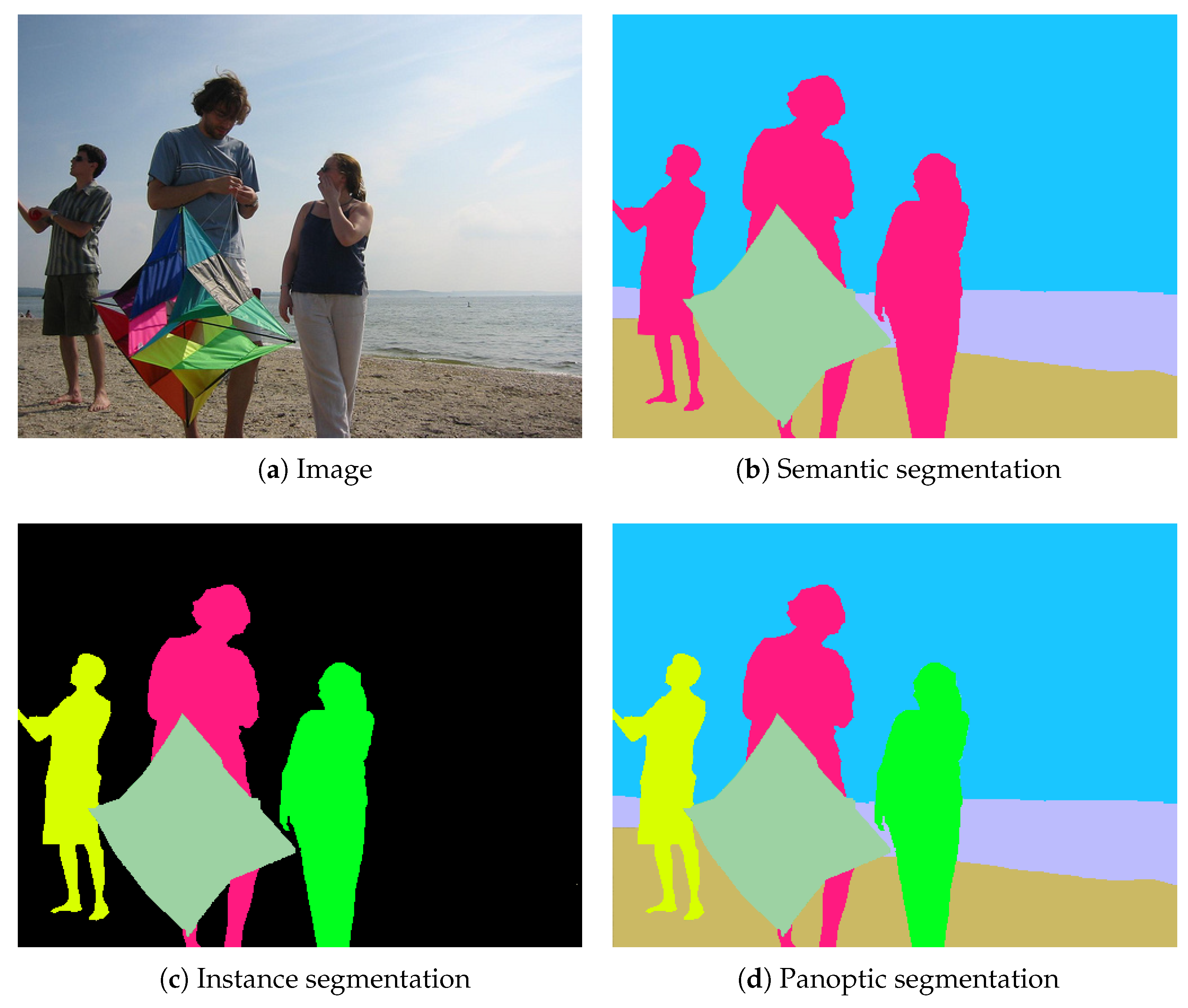
Image segmentation is one of the major tasks in the field of computer vision. Currently, image segmentation is used in a wide range of fields, such as medical image analysis, autonomous driving, security, satellites, and aerial photography, and it is expected to be used in even more fields in the future. Image segmentation is divided into three main categories, as shown in Figure 1. The first category is semantic segmentation, which predicts the class of each image pixel but does not distinguish instances within the same class. The second category, instance segmentation, distinguishes instances within the same class but does not predict all the image pixels; it predicts one type of object (the foreground) rather than the others in the background. Lastly, panoptic segmentation [1] combines semantic and instance segmentation. It predicts the foreground and background in the image while distinguishing instances of the same class.
Concomitant with increasing interest in the foreground and distinguishing identical instances within the same class, instance segmentation is actively being researched. Accuracy-focused models include Dual-Swin-L [2], Segmenting Objects with Transformers (SOTR) [3], and mask region-based convolutional neural network (Mask R-CNN) [4], and speed-focused models include CenterMask [5], SOLOv2 [6], BlendMask [7], YOLACT [8], and YolactEdge [9]. Typically, a performance comparison with other methods is presented in the paper in which a method is proposed. When only a few or no methods are compared in the original paper, researchers have to compare the performance of all methods based on the performance of each method reported in its original paper. This makes comparison challenging because each method uses different hardware in the inference environment. We found no studies comparing the performance of instance segmentation models. This study addresses this issue by benchmarking state-of-the-art instance segmentation models.
The ultimate aim of our study is to compare performance differences between platforms by mounting models learned on workstations to mobile and analyzing the main factors contributing to performance differences. Thus, this study investigates state-of-the-art instance segmentation models, compares their performance in fixed workstation environments, and estimates their potential in mobile environments as a prior study for future work. To the best of our knowledge, this is the first instance segmentation benchmarking study, and we make the following contributions. We compare the average precision (AP) and inference speed (frames per second; FPS) of each model in a fixed environment using GTX 1080 Ti and RTX 3090 GPUs. In addition, we analyze the structure of these models to specify a model that can operate in a real-time environment. We also compare the masked image and analyze the mask quality according to the AP through the qualitative results. Finally, we discuss the analysis results and present our findings.
The most important results and findings from our analysis are as follows: (1) All speed-focused models capable of real-time inference use the feature pyramid network (FPN) structure. Therefore, from the results on network structures released thus far, an FPN can be considered when designing a real-time model. (2) There is a trade-off between AP and FPS. Therefore, an appropriate balance between speed and accuracy should be considered for real-time use. (3) The higher the GFLOPS, the faster the inference speed, but it does not increase proportionally. (4) Based on the results of (3), it is difficult to predict the inference speed on mobile solely with GFLOPS; consequently, subsequent studies are needed to find and analyze the main factors contributing to performance differences between platforms.
2. Related Work
The performance of mobile AI accelerators is improving rapidly every year, and thus attempts to utilize deep learning models on mobile hardware continue to increase. Ignatov et al. [11] benchmarked the performance of mobile chipsets that support hardware acceleration for AI inference for deep learning models. They selected networks that performed vision tasks to present the relative inference performance of mobile SoCs in 16-bit floating-point (fp-16) networks. They also presented the relative inference performance in 32-bit floating-point (fp-32) networks so that the SoCs performance can be compared with that of Intel CPUs and NVIDIA GPUs. Finally, they presented the relative performance of SoCs in 8-bit integer-quantized networks.
With the increasing amounts of data available and the rapid improvements in the computing performance of hardware, deep learning models are achieving many successes in various areas. Applying deep learning to mobile or embedded devices is gaining increasing attention, and comparing performances by benchmarking the AI performance of each device has also been adopted as an important challenge. Luo et al. [12] proposed the AIoTBench, a benchmark suite for evaluating inference performance on mobile and embedded devices. They also provide data that compare and rank the performance of five mobile devices in representative heavy and light networks.
Deep neural networks (DNNs) are achieving remarkable results in many computer vision tasks. The literature shows that researchers have conducted many studies aimed at designing efficient and accurate networks. Bianco et al. [13] compared the performance of more than 40 state-of-the-art DNN architectures for image recognition tasks. They provide performance indices such as the recognition accuracy, inference speed, and memory usage of DNNs running on two systems with significant differences in computing power, and analyze the association between these performance indices.
With the use of CNNs, many studies have progressed on object detection tasks. Although some state-of-the-art object detectors have been shown to be sufficiently fast to run on mobile devices, it may be difficult for practitioners to determine which architecture is suitable for their purposes. Therefore, Huang et al. [14] conducted experiments and analyzed the major factors affecting the trade-off between the inference speed and detection accuracy of modern object detectors. They presented measurements such as the architecture’s inference speed, detection accuracy, and memory usage, which depend on variables such as feature extractors, image resolution, and the number of proposals in a fixed hardware environment.
The training of deep learning models is computation-intensive, and new and better hardware and software platforms are being proposed to train and deploy more sophisticated models. Thus, Wang et al. [15] introduced ParaDnn, a parameterized benchmark suite for benchmarking deep learning platforms. They benchmark Google TPU, NVIDIA GPU, and Intel CPU platforms with six DNN models to compare the execution time for training according to various specifications of hardware and software.
Many models and algorithms have been proposed in computer vision research, and the importance of datasets and benchmarks has also been demonstrated as a means of quantitatively evaluating and comparing them. Ammirato et al. [16] presented a new public dataset that focuses on robots performing vision tasks in difficult indoor environments. The dataset contains more than 20,000 RGB-D images and 50,000 object 2D bounding boxes for instances captured in nine unique scenes. Perazzi et al. [17] presented a new video object segmentation benchmark dataset, called the Densely Annotated Video Segmentation (DAVIS), consisting of high-quality sequences at full HD resolution. They compared state-of-the-art methods with their proposed three metrics using DAVIS, which includes common situations such as motion blur and occlusion that may arise from video object segmentation tasks.
3. Background
3.1. Feature Pyramid Network (FPN)
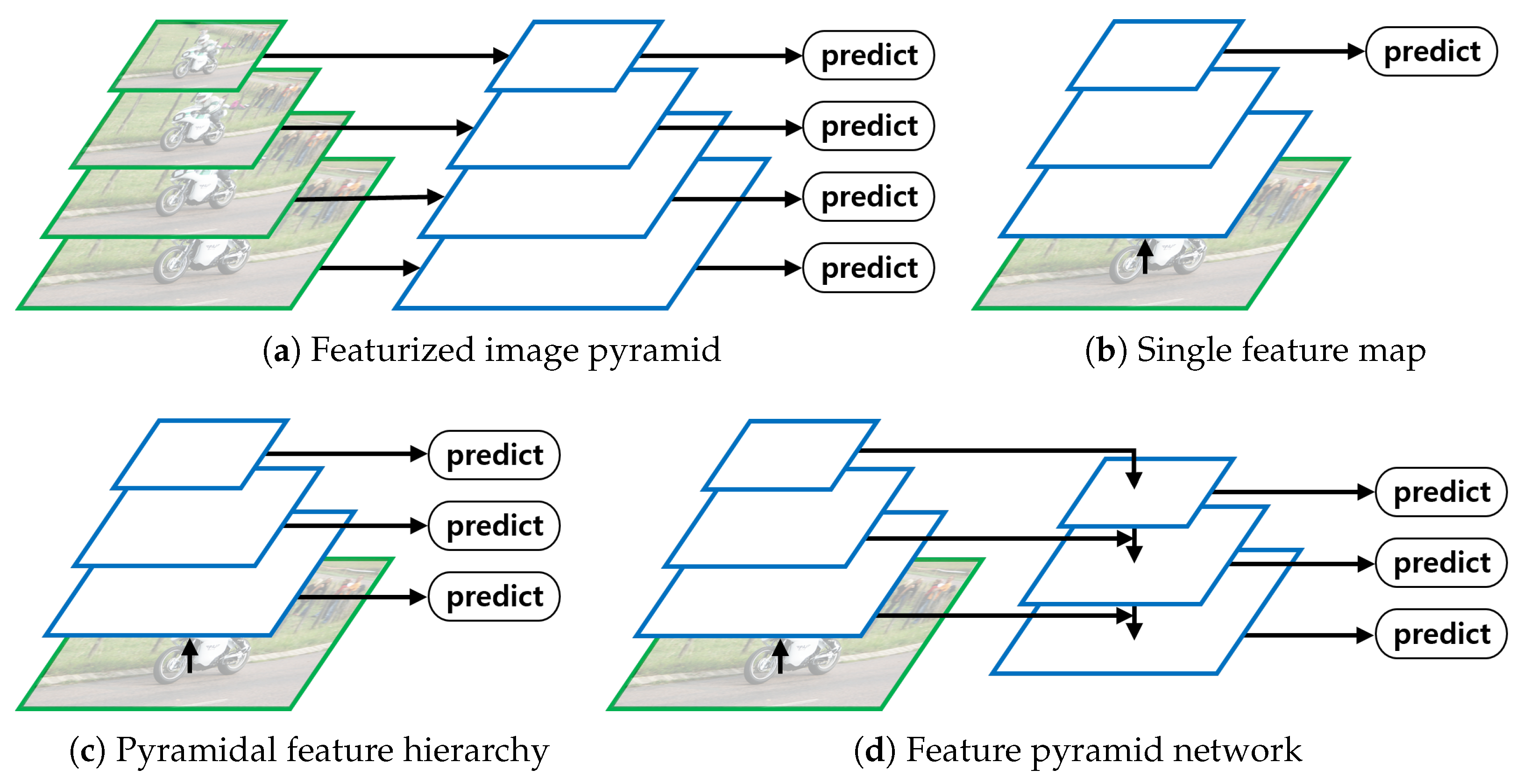
Detecting objects of various sizes existing in an image is a key issue in the object detection task. Although various methods have been proposed that can adequately detect an object regardless of its size, it is being argued that the inference speed of current models is slow and that they are memory-intensive [18]. To address this issue, a method has been proposed for detecting objects of various sizes while being less computationally expensive through the FPN [18] (Figure 2d).
The featurized image pyramid method resizes input images to various sizes and extracts feature maps from each resized image, such that feature maps of various sizes can detect large and small objects well. However, because a CNN is applied to each resized image, the method is computation- and time-intensive. The single feature map method extracts feature maps from an input image and detects objects only with the final feature map. Its learning and inference are fast because a CNN is applied only once. However, its performance is poor because only the final feature map with low resolution is used. The pyramidal feature hierarchy method extracts feature maps from an input image and performs object detection on each extracted feature map. Although detection is performed while maintaining information about small objects, the feature map of the already generated upper level is not reused and does not reflect the low-resolution feature with rich semantic information. FPN first extracts feature maps of various scales through bottom-up paths. Then, through the top-down pathway, the low-resolution feature map combines bottom-up feature maps with lateral connection while increasing the resolution. The authors of [18] argue that by combining feature maps with rich semantics information in a top-down manner and feature maps that preserve location information in a bottom-up manner, strong feature maps can be rapidly generated at various scales.
3.2. Vision Transformer
Self-attention-based structures have been widely used in the field of natural language processing (NLP). In particular, methods similar to Bidirectional Encoder Representations from Transformers (BERT) [19] that are pretrained on large text corpora and fine-tuned on small task-specific datasets are dominant. Although the Transformer [20] structure has been actively used as the main standard in the NLP field, it has rarely been used in the vision field. As transformers have been successfully utilized in NLP, many scholars have attempted to apply them to the vision field as well. In most cases where attention is used in vision task, it is applied in conjunction with a CNN or used in a way that replaces a specific element of the CNN. However, Dosowski et al. [21] developed a vision transformer (ViT) that could achieve state-of-the-art performance in image classification tasks, revealing that dependence on these CNNs is not essential and that transformers can replace them. Researchers have moved away from the existing limited attention mechanism and replaced most of the CNN structure with a Transformer while designing the model to be similar to Vaswani’s original transformer [20]. The Transformer receives a one-dimensional token-embedding sequence as an input. Therefore, the original three-dimensional image is flattened into one-dimensional patches. The patches are mapped to a constant latent vector (patch embedding) through trainable linear projection, and position embedding is applied to maintain location information. In addition, similar to the BERT [CLS] token [19], one learnable [class] token is added to the front of the embedded patches to perform classification. When pre-training was conducted with datasets of various sizes and evaluated on many benchmark cases, the ViT was very efficient in terms of the pre-training calculation cost, and in most benchmark cases, the performance was similar or superior to those of the state-of-the-art approaches and the pre-training cost was low.
3.3. Non-Maximum Suppression (NMS)
Most object detection algorithms generate bounding boxes (bboxes) with high scores around the object’s location. NMS is a technique that removes all bboxes around the same object except for the bbox with the highest score. NMS is an essential component of object detection and instance segmentation, and research is being conducted to improve the speed of traditional NMS. YOLACT’s Fast NMS [8] removes more anchor boxes than NMS, and hence it causes some performance degradation, but unlike NMS, it performs matrix operations, and hence it can be calculated more quickly by GPUs. SOLOv2’s matrix NMS [6] can handle 500 masks with a simple Python implementation in less than 1 ms by simultaneously solving the problems of hard removal and sequential operations.
3.4. NVIDIA TensorRT
TensorRT [22] is a software development kit that improves the speed of inference in NVIDIA GPUs by optimizing the trained deep learning model. To ensure optimal inference performance on NVIDIA platforms, TensorRT automatically applies network compression, network optimization, and GPU optimization technologies to models trained in most deep learning frameworks and is widely used in artificial intelligence, autonomous machines, high-performance computing, and graphics. TensorRT also supports optimal deep learning model acceleration with quantization, precision calibration, graph optimization, and kernel auto-tuning.
3.5. Quantization
Most of the interior of the neural network model is composed of weights and activation functions, and it is represented using 32-bit floating-point numbers to improve the accuracy of the model. In mobile, AI-device, and embedded environments, inference using deep learning models is difficult because memory, performance, and storage space are limited. Therefore, in recent years, many studies related to model weight reduction have been conducted in deep learning. Quantization refers to the process of converting a floating-point type into an integer or fixed-point number. Reducing the number of bits by mapping the 32-bit floating-point data type to a certain range leads to reductions in memory and model size as well as increases in inference speed and power consumption efficiency. There are two types of quantization techniques: (1) post-training quantization, which is learning with a floating-point model and then quantizing the resulting weight values to minimize quantization errors, and (2) quantization-aware training, which performs quantization during weight optimization in training. In the post-training quantization method, both dynamic quantization and fusion quantization are performed. Dynamic quantization quantizes only the weight of the model and dynamically quantizes activations during inference, whereas static quantization combines the activation and its layer to reduce the context-switching overhead of the model. Quantization-aware training performs clamping and rounding tasks by placing a fake quantization module in the model during training, which can be changed to the integrated model with values such as scale and zero points stored in the module when training is completed.
4. Review Method
We divided the target methods into accuracy-focused and speed-focused models. Mask R-CNN [4] is the most basic model in the field of instance segmentation. It was therefore selected as a baseline accuracy-focused model for comparison with the other models. SOTR [3] and Dual-Swin-L [2] were chosen to represent the accuracy-focused models because the Transformer structure has been successfully applied in the field of instance segmentation. CenterMask [5], YOLACT [8], YolactEdge [9], BlendMask [7], and SOLOv2 [6] were designed for real-time use and provide a trained model; hence, they were used to exemplify the speed-focused models.
4.1. Accuracy-Focused Models
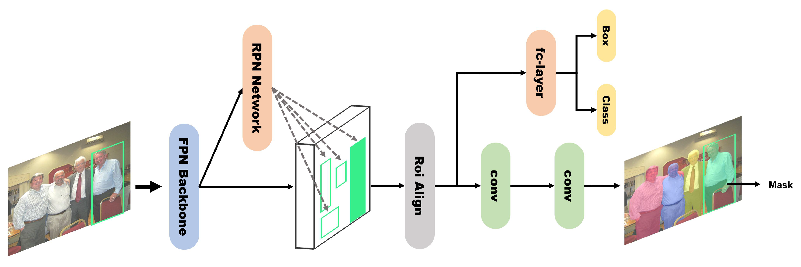
Mask R-CNN [4] is a model for two-stage instance segmentation. It creates a region of interest (RoI) candidate in the first step and classifies and segments the RoI in the second step (Figure 3). As an extension of Faster R-CNN [23], branches for mask prediction in each RoI are added in parallel to the existing branch for classification and bbox regression. The structure of the head varies depending on the backbone, and when a ResNet-FPN backbone is used, the region proposal network (RPN) produces an RoI using a feature pyramid generated through the pre-processed input image. Faster R-CNN is a model for object detection, and the RoIPool of the RPN has a significant adverse effect on the pixels of the prediction mask due to the misalignment between the RoI and feature when quantizing the RoI into a feature map. To segment the pixel units, the RPN replaces the RoIPool of the existing Fast R-CNN RPN with RoIAlign, which contains location information using bilinear interpolation. Feature maps extracted through RoIAlign are delivered to the classification and bbox regression branches through the fully connected layer to obtain the final class scores and bbox, and to minimize the loss of spatial information in the mask branch, a small fully convolutional network [24] is used instead of an fc-layer to improve the mask performance.
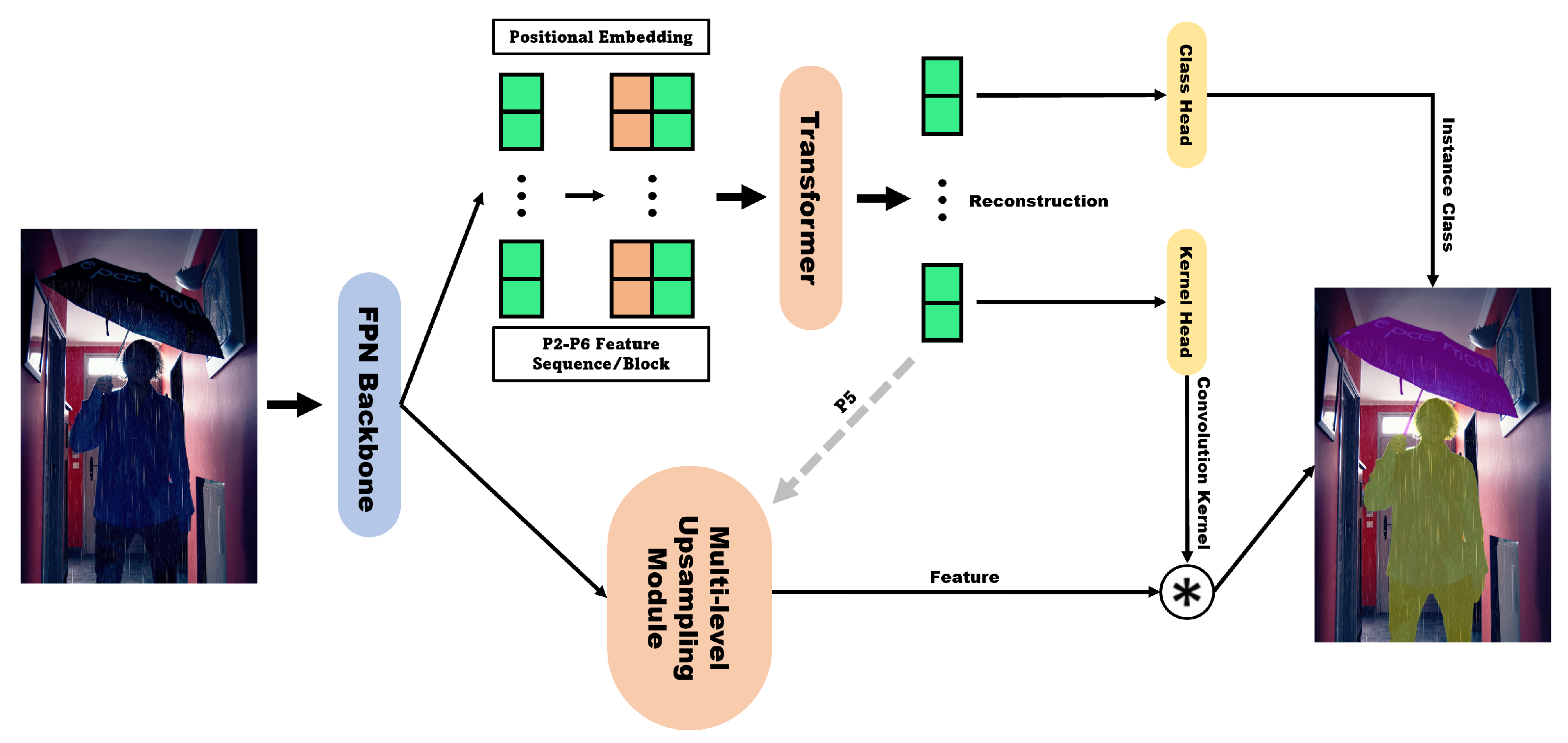
SOTR [3] has been proposed as a segmentation model combining an FPN backbone and a transformer network. SOTR consists of a process that predicts the category of each instance through a transformer and a process that generates a dynamic segmentation mask by computing the dynamic convolution kernel produced by the kernel head and features generated by the multi-level upsampling module (Figure 4). Many instance segmentation methods based on CNNs have adopted a top-down approach that first detects objects and then predicts segmentation masks. The authors who presented SOTR [3] noted that this approach has advantages in terms of translation equivariance and location information, but for large objects, the receptive field of a CNN may lead to poor results when connecting high-level features to instances. They also stated that the performance of the object detector determines the inference speed and mask quality of the image, which can lead to poor performance when processing complex images. To overcome these issues, SOTR adopts a bottom-up approach and dynamically creates masks while learning position-sensitive features regardless of the location and scale of the bbox and grouping post-processing.
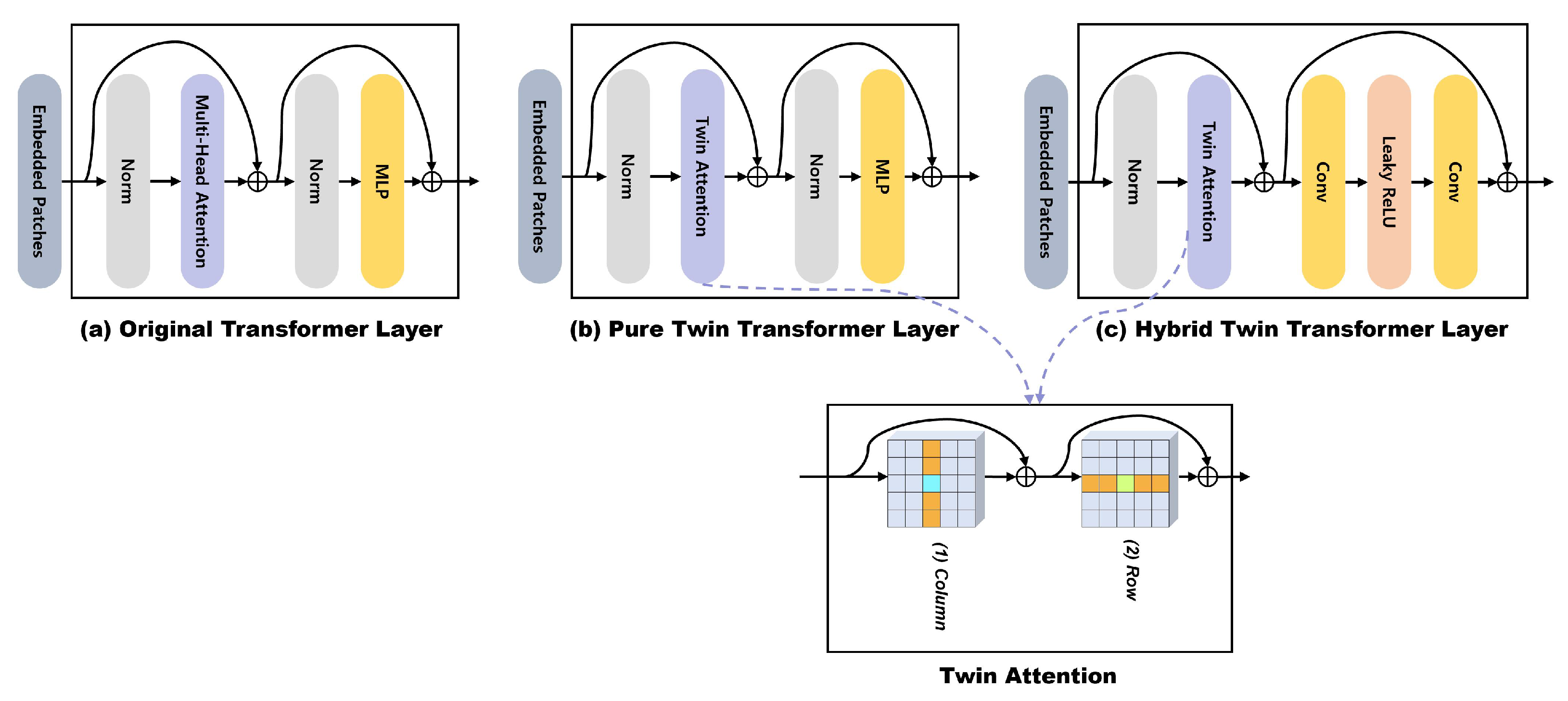
In the transformer network, to replace the original transformer layer using multi-head self-attention [20] (Figure 5a), researchers proposed the pure twin transformer layer and hybrid twin transformer layer, which are based on twin attention and shown in Figure 5b,c. Transformers receive some feature maps generated by the FPN backbone. After the transformer, there is a class head for predicting the instance class and a kernel head for creating the convolution kernel dynamically. The multi-level upsampling module receives some feature maps from the FPN and the P5 features reconstructed by the transformer to create a final mask through dynamic convolution operations.
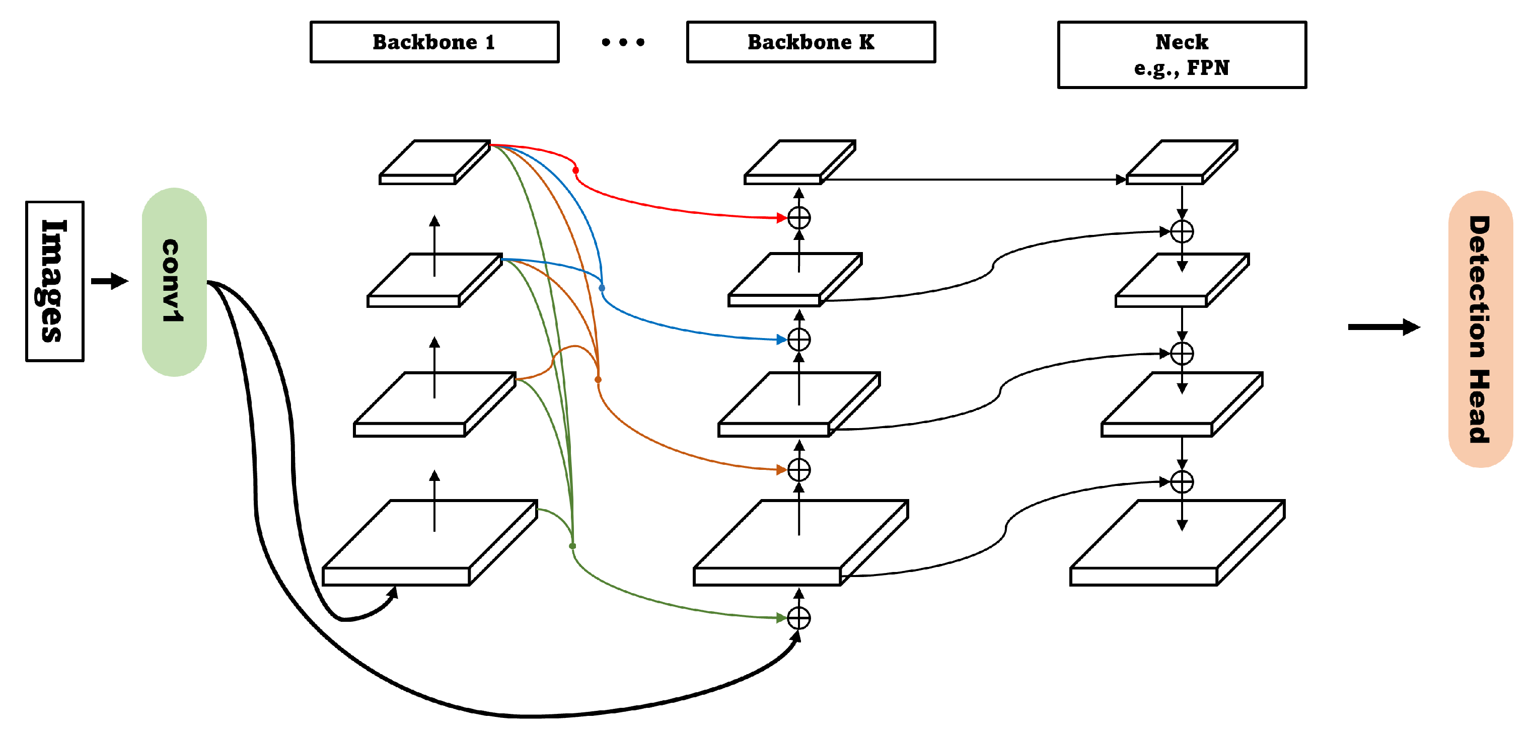
Dual-Swin-L [2] is a multi-backbone network that combines two same identical large Swin transformer networks [25] (Figure 6). It is designed to perform object detection efficiently by combining high- and low-level features (Figure 7). CBNetV2 [2] is a dense higher-level composition that efficiently combines high- and low-level features and an auxiliary supervision to optimize the training process of the model. Therefore, Dual-Swin-L not only reduces training time by 6x compared to Swin-L, but it also improves performance without additional training data through multi-scale testing.
Prior to the proposal of the Swin transformer, which is the main network of Dual-Swin-L, the original transformer [20] was designed for NLP, but it has been applied in the vision field as the ViT [21]. However, the authors who presented the Swin transformer noted that the ViT is not appropriate to use as a backbone for dense vision tasks or when the image resolution is high, because the global self-attention of the ViT throughout the patch (which is MSA) is computation intensive when the resolution of the input image is high and only has single-resolution feature maps.
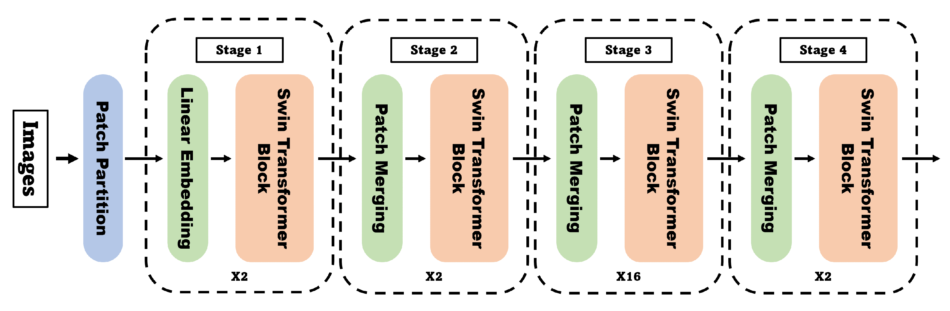
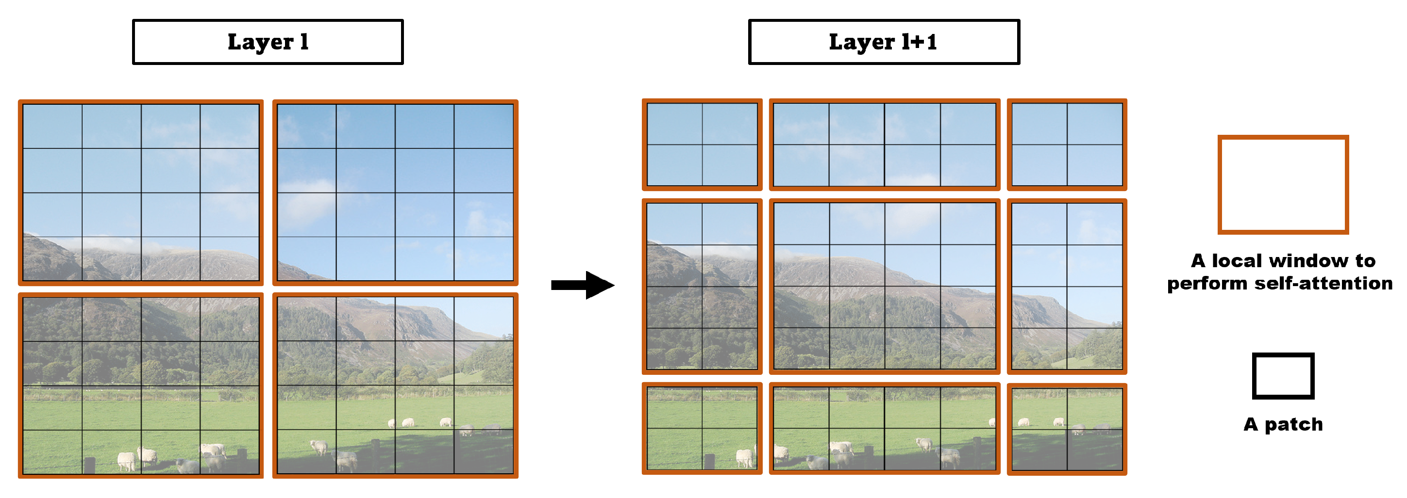
Therefore, the Swin transformer [25] network has a structure in which each patch is divided into windows, and self-attention is performed only within the corresponding window (W-MSA). However, as the W-MSA module performs self-attention only on fixed windows, the connectivity between windows is poor, limiting the modeling performance; hence, the authors proposed shifted window-based self-attention (SW-MSA), which shifts this window and performs self-attention once more. As W-MSA and SW-MSA perform self-attention only within the window, unlike MSA, it is possible to reduce the amount of computation efficiently. As the stages progress, patches merge and use a window consisting of a larger patch, which is responsible for a larger receptive field in the image (Figure 8). This means that the network is trained to detect both small and large objects well.
4.2. Speed-Focused Models
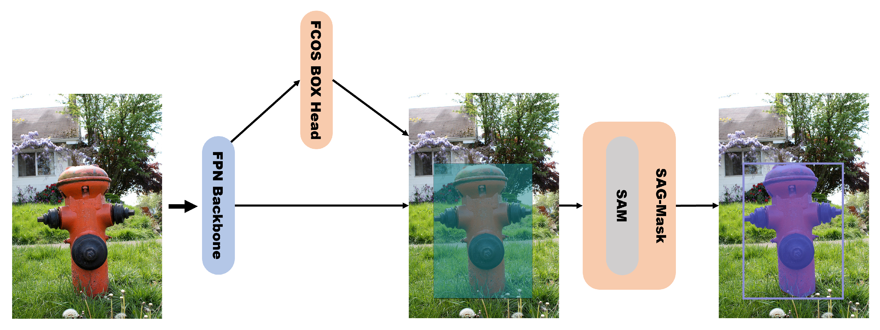
CenterMask [5] was proposed as an anchor-free instance segmentation model. It is an architecture with a spatial attention-guided mask (SAG-Mask) branch added after the anchor-free one-stage object detector (FCOS) [26] and uses an FPN backbone (Figure 9). When CenterMask was proposed, few studies had considered the inference speed, and the accuracy was lower than that of Mask R-CNN [4]; hence, CenterMask was designed to improve both accuracy and speed. The authors who presented CenterMask [5] argued that anchor-box-based object detectors depend strongly on predefined anchors; hence, when too many anchor boxes are created, they not only cause imbalances between positive and negative RoI samples, but also increase the computational costs. To overcome the shortcomings of these anchor boxes, an FCOS is used as an object detector in CenterMask in the first stage, which is anchor-free. In mask prediction, each RoI pooling operation should be allocated considering the RoI scale when extracting the features from each RoI. However, as RoIAlign proposed for Mask R-CNN [4] does not consider the input scale, the authors [5] designed a scale-adaptive RoI assignment function suitable for an FCOS.
When CenterMask was proposed, attention methods were widely used for object detection because they can help the model extract more important features while suppressing unimportant features. Channel attention focuses on what important information is in the channels of the feature maps, whereas spatial attention focuses on where the important information is located in the feature maps. The spatial attention module (SAM) inside the SAG-Mask helps to predict the mask by emphasizing meaningful pixels while reducing noise in Figure 9. The FCOS receives feature maps from the FPN backbone and predicts the bboxes. The bboxes received from the FCOS are used to extract features inside the predicted RoI through the scale-adaptive RoI assignment function, and the final masks are output through the later SAG-Mask, which consists of convolutional layers, a spatial attention module, upsampling processes, and other processes.
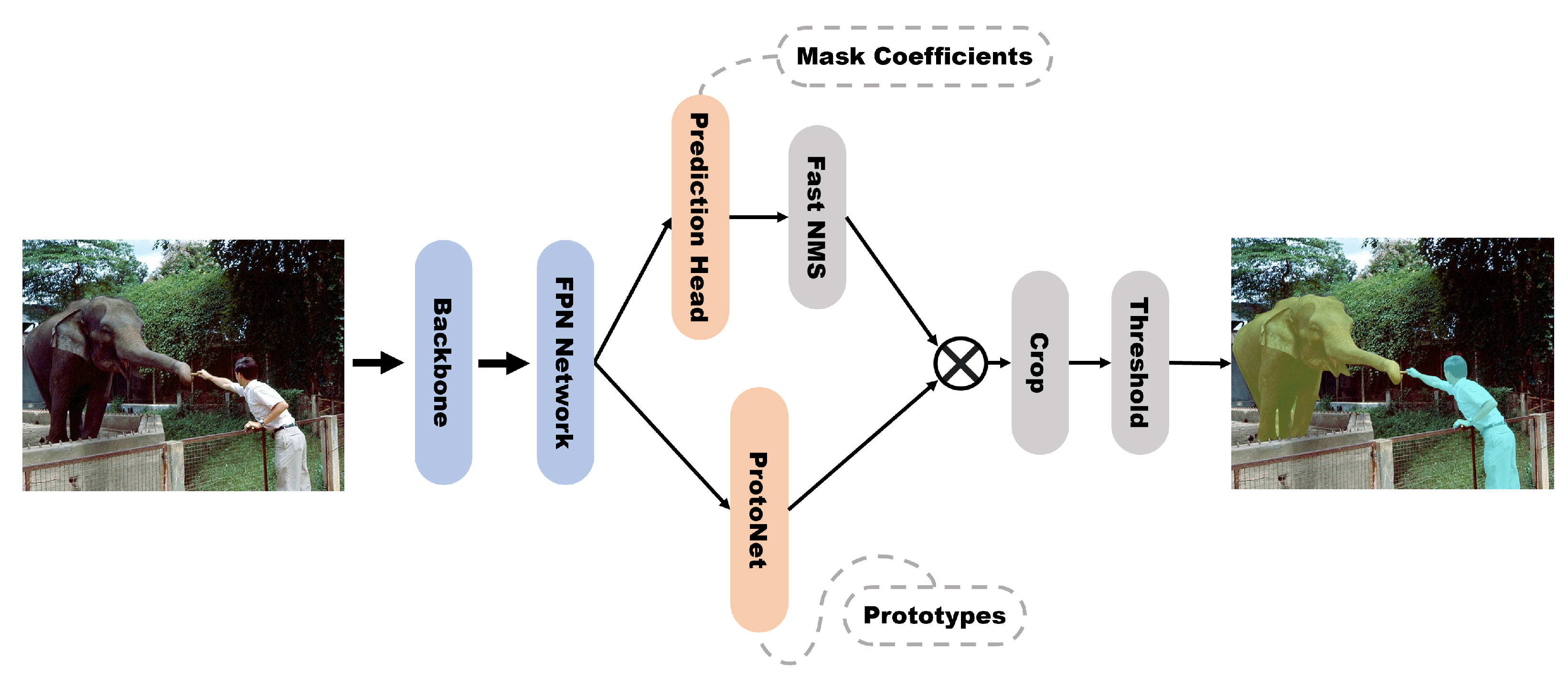
YOLACT [8] was proposed as a one-stage instance segmentation model separated by two parallel subprocesses: (1) the generation of a prototype mask set and (2) the prediction of mask coefficients per instance (Figure 10). The basic model is a modification of RetinaNet [27], a one-stage object detection model. In YOLACT, instance segmentation processes were parallelized with a ProtoNet and a prediction head to add mask branches without feature localization steps.
In the prediction head, the feature maps from the FPN are input and sent to the class, box, and mask coefficient branches through convolution. ProtoNet receives the deepest feature map of the FPN, P3, as an input and generates a predefined number of prototype masks, but each mask does not activate (localize) one specific instance. Therefore, for each instance that is not erased via Fast-NMS, YOLACT performs a mask assembly that creates a mask by linearly combining the prototype mask and mask coefficient. The final mask is generated by cropping outputs of the mask assembly based on the predicted bbox and by thresholding.
The author of [8] also proposed Fast NMS, which speeds up with slight degradation of AP, instead of the standard NMS used in Mask R-CNN. The Fast NMS is as follows: when a reference anchor box is compared to other anchor boxes with higher confidences than itself, if the compared anchor box with the largest intersection-over-union (IoU) value is less than the threshold, the reference anchor box is not erased. In standard NMS, when an anchor box is erased, it is no longer compared to any other anchor box. However, in Fast NMS, the already erased anchor box continues to be used for comparison to erase other anchor boxes. Fast NMS has a slightly worse performance because it removes more anchor boxes than NMS, but matrix operations can be performed using a GPU, resulting in significant speed improvements.
YolactEdge [9] is a model based on YOLACT [8] that has two fundamental improvements at the system and algorithm levels so that it can perform inferences in real time on edge devices. The system was improved by using an NVIDIA TensorRT [22] to adjust the balance between speed and accuracy systematically while quantizing network parameters to 8-bit integer (int-8) or fp-16, which is the precision of a smaller bit range. A wider precision range requires more time for calculation and thus is more accurate. In addition, if the weights of the model components have different precision ranges, the balance between speed and accuracy depends on the components. Therefore, to maximize FPS without loss of accuracy, YolactEdge explored the optimal combination of int-8 and fp-16 weights for each component of the YOLACT by applying TensorRT.
In particular, changing the prediction head to int-8 significantly decreases the segmentation accuracy. Hence, the authors converted all components except the predicted head and FPN to int-8, quadrupling the speed with the calibration step.
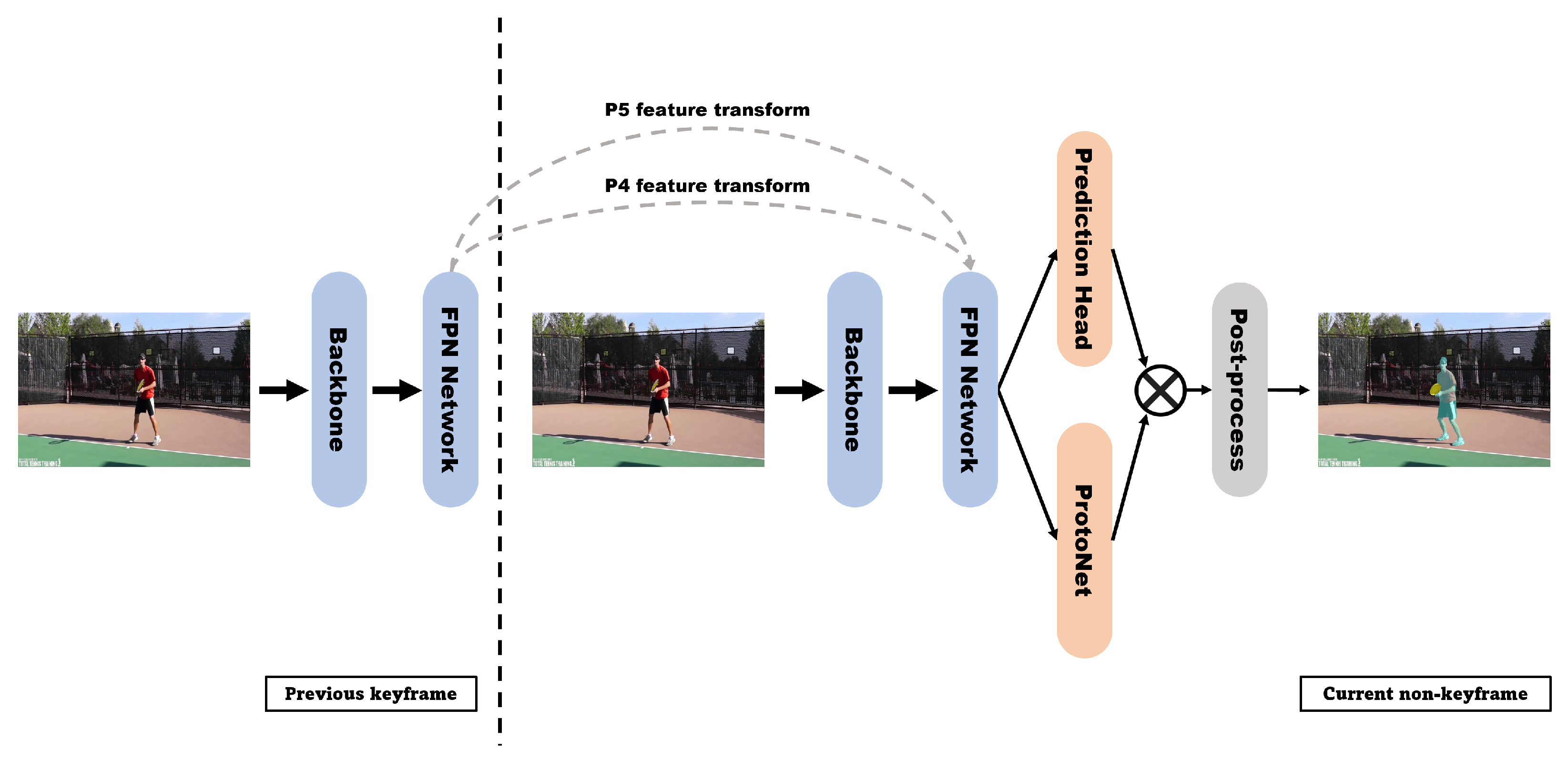
When YolactEdge was proposed, other real-time instance segmentation methods dealt with only static images. The authors who presented YolactEdge [9] argued that real-time applications are much more important in video applications, which require low latency and real-time inference. Therefore, the model was switched from static image processing to video processing, and training was performed using the YouTube Video Instance Segmentation dataset [28]. The improvement at the algorithm level involves using temporal redundancy when dealing with videos. In the keyframe case, backbone and pyramid features are computed, but in the non-keyframe case, only some of the backbone and pyramid features are computed and some of the pyramid features are transformed via partial feature transform from the nearest previous keyframe in time (Figure 11). Through this process, the speed of YolactEdge is greatly accelerated because it avoids calculating the most expensive part of the backbone.
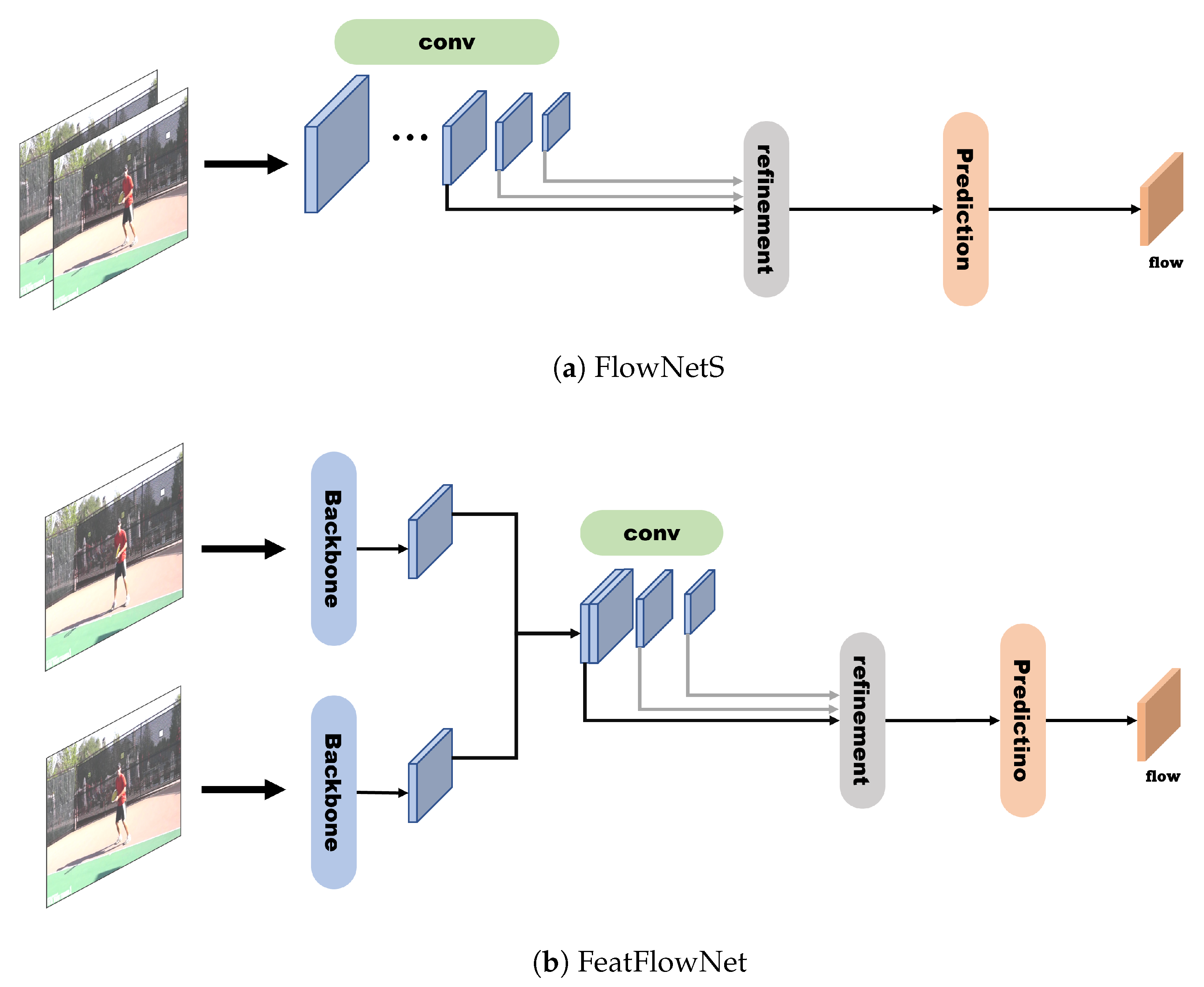
To transform features quickly, object motion must be efficiently estimated, and thus FeatFlowNet, a modified network that follows the architecture of existing FlowNetS [29] (Figure 12a) but reuses the backbone’s features and uses fewer convolution layers, was proposed (Figure 12b). In the feature transformation process, the flow map between the previous keyframe and current non-keyframe is estimated through FeatFlowNet; then, the features are transformed from the previous keyframe to the current non-keyframe through inverse warping, resulting in much faster calculations and identical performance.
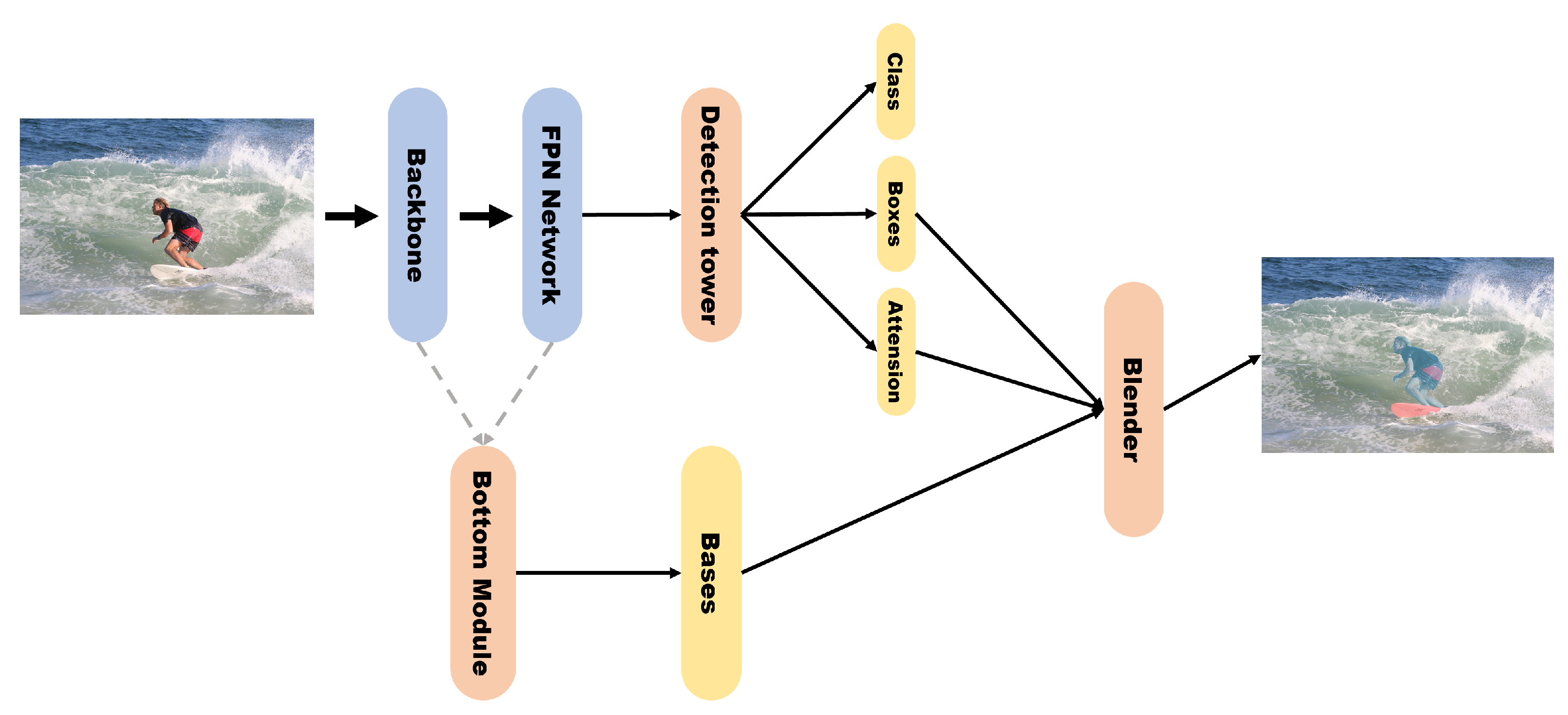
Blendmask [7] was proposed as an instance segmentation model that improves mask prediction based on an FCOS detector [26] with minimal modifications. The authors who presented Blendmask [7] argued that high-level features represent semantic information about instances more effectively than low-level features because the former have larger receptive fields than the latter, and that low-level features have the advantage of including more detailed information than high-level features without losing location information. Hence, the authors mixed the bottom-up and top-down approaches. Blendmask consists of two blocks: an FCOS detector that predicts the class and bbox of the instance; a mask branch that predicts the score maps and instance attentions, and then merges the scores with attentions (Figure 13).
Detection towers use the feature maps of an FPN to perform classification. Next, attention maps and bboxes are generated by adding a single convolution layer to each tower. The bottom module selectively receives the backbone or FPN features to generate score maps called bases. Chen et al. [7] experimentally found that the AP of FPN features is higher than that of backbone features. For each instance predicted in the detector module, the blender module divides the bases with bboxes and linearly combines the attention maps to output the final mask.
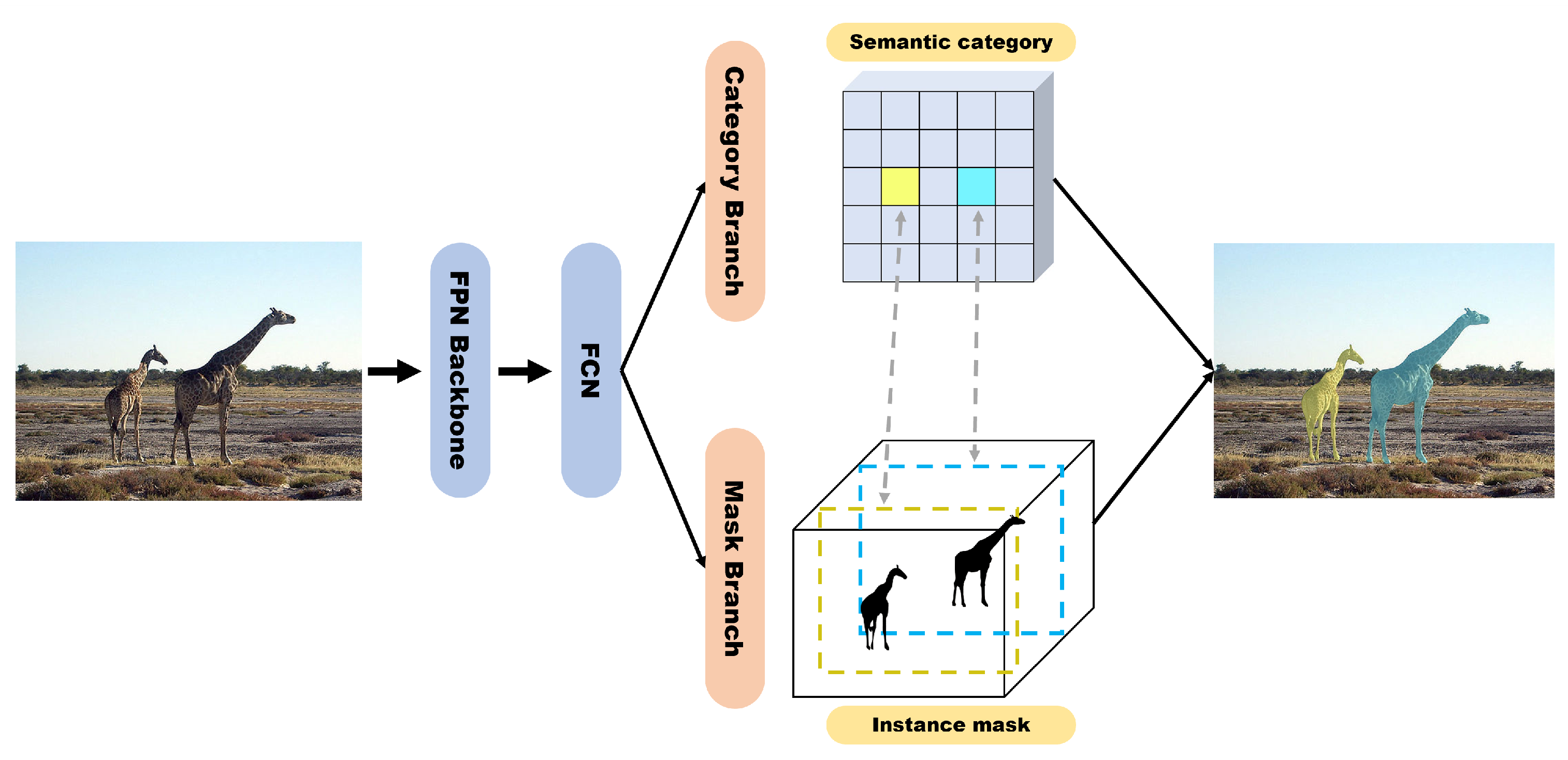
SOLOv2 [6] was proposed as a model for improving the head part and NMS of segmenting objects by locations (SOLO [30]). SOLO introduced the concept of assigning categories to pixels inside instances according to the location and size of instances called instance categories. Before SOLO, a top-down method that first detects objects and then segments them and a bottom-up method that first predicts the class of the embedding vectors and then groups the same instances together were used. The authors who presented SOLO [30] argued that these two approaches have shortcomings, because they heavily depend on the detector performance or embedding learning and grouping processing. Therefore, the SOLO model was designed with the objective of directly segmenting the instance mask.
SOLO is simply composed of a category branch and mask branch, and when the center of the object to be predicted enters a specific grid cell, the cell predicts the category and instance mask of the object (Figure 14). The mask branch uses a CoordConv operator with two additional channels with information on the x–y coordinates in pixels to increase spatial variance. In addition, instead of using the existing vanilla head, the decoupled head, which predicts the x-axis and y-axis separately, is used to further improve performance. Finally, when the segmentation result corresponding to each grid cell is output, the final mask is created by removing the duplicate mask via NMS.
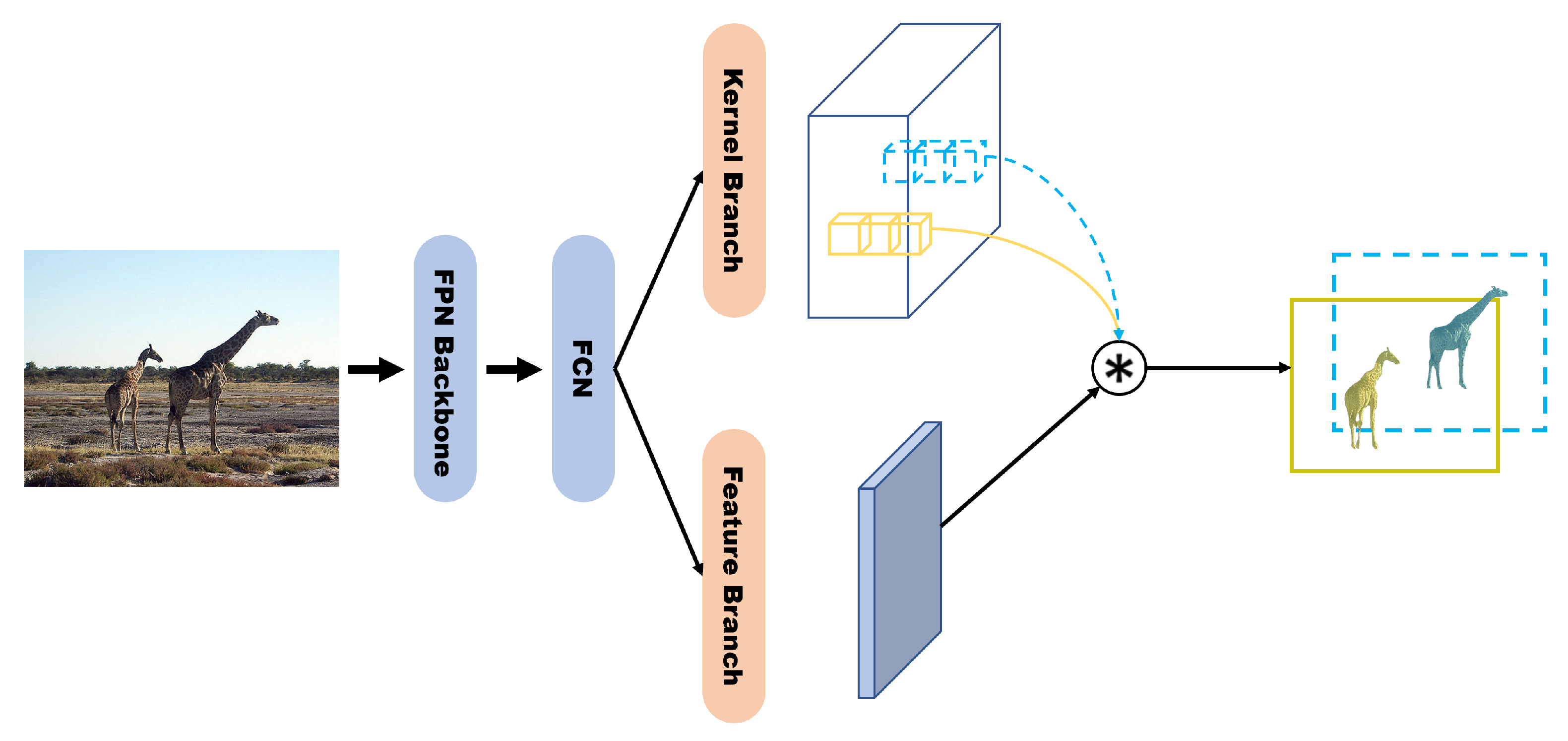
SOLOv2 [6] divides SOLO’s mask branch into a kernel branch that performs kernel learning and a feature branch that performs feature learning (Figure 15). In the kernel branch, the mask kernel is dynamically generated for the input. In the feature branch, the FPN feature maps are all upsampled to 1/4 of the input size. Then, all the features are added element-wise and 1 × 1 convolution is performed to create unified mask features. Next, the outputs of the kernel and feature branches are convoluted to obtain an instance mask. Finally, a matrix NMS, which is an improved version of the standard NMS, is used to generate the final mask.
5. Experiments
The COCO object detection dataset is a large-scale image dataset designed to advance state-of-the-art techniques for the object detection task. In our experiments, we used the MS COCO 2017 instance segmentation dataset [10]. This dataset includes 123K images with 80 class instance labels. The original images in the inference results were obtained from the val2017 dataset (5K images). To evaluate the performance of the methods, we used the metrics of COCO [10]. The evaluation metrics were AP; AP; AP, AP, and AP (AP at different scales).
If T is mask, IoU is the intersection of the mask pixels, and if T is box, IoU is the intersection of the bounding boxes. Thresholds is the threshold range of the IoU and has a step size of 0.05 from 0.5 to 0.95
Each target method is provided as a trained model using a different backbone [2,3,4,5,6,7,8,9]. When selecting the trained models, we selected those with the highest AP as the accuracy-focused models; those with the highest AP in real-time as the speed-focused models; and the Mask R-CNN model is from the Detectron2 [31] library. The evaluated FPS is the result of an average of ten inference runs on a single GPU. The test environment was divided into two environments according to the type of GPU:
- (1)
- RTX 3090 + Intel i9 10900X + CUDA 11.3 + PyTorch 1.10.1;
- (2)
- GTX 1080 Ti + Intel i9 10900X + CUDA 10.2 + PyTorch 1.10.1.
5.1. Quantitative Results
5.1.1. Accuracy Rate
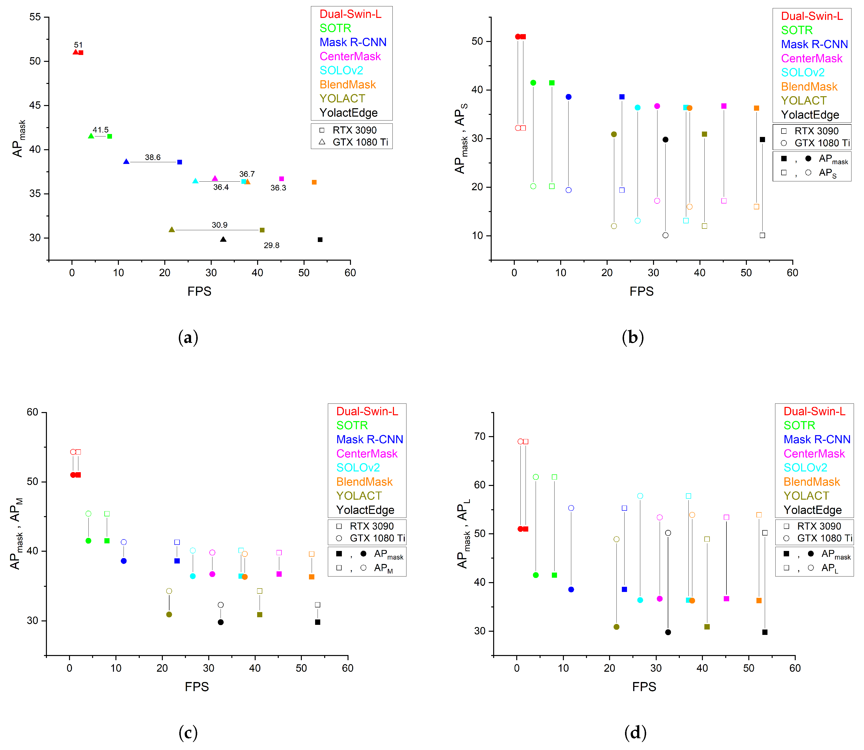
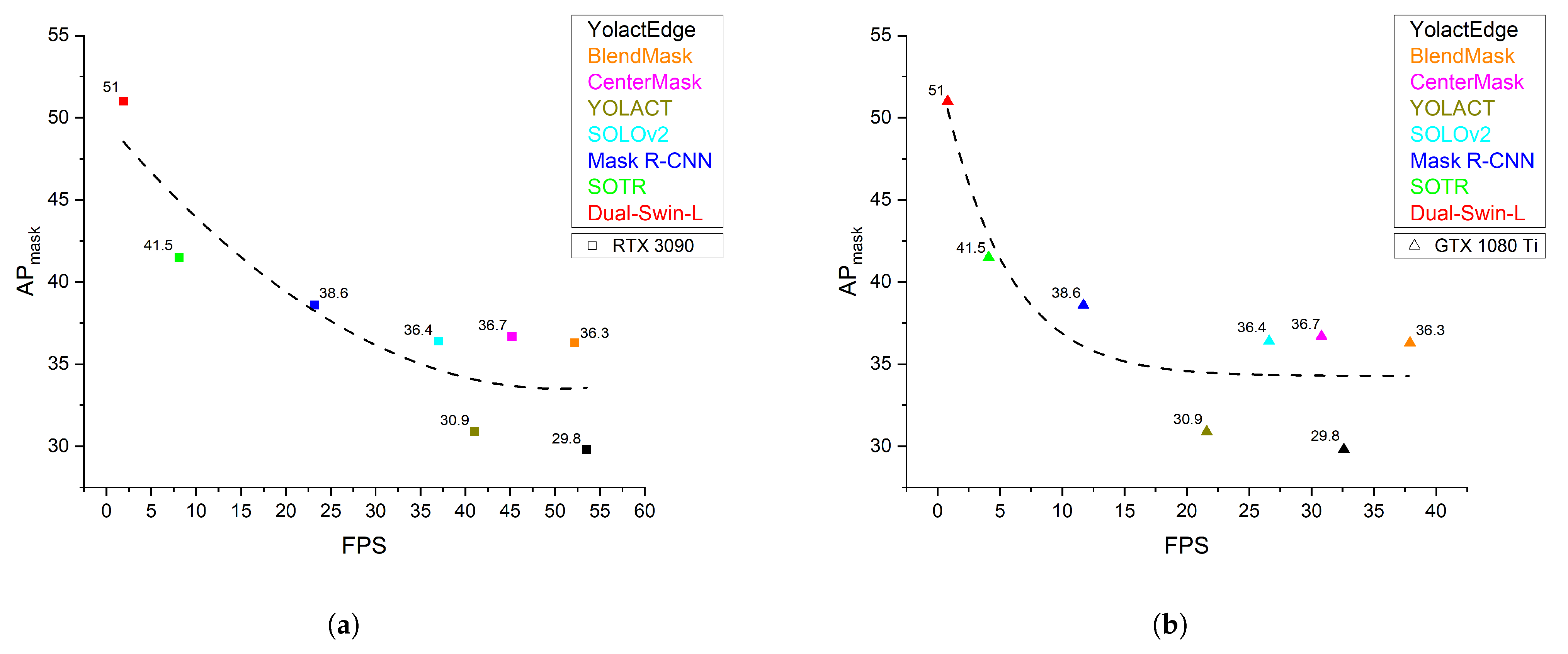
The results of the state-of-the-art instance segmentation models on the MS COCO val2017 dataset are presented in Table 1. They show that the AP results were the same even when a different inference GPU was used. Among the accuracy-focused models, Dual-Swin-L achieved the highest AP of 51.0, followed by SOTR (41.5), and Mask R-CNN (38.6). Among the speed-focused models, CenterMask achieved the highest AP of 36.7, followed by SOLOv2 (36.4), BlendMask (36.3), YOLACT (30.9), and YolactEdge (29.8). YolactEdge achieved 29.9 AP when TensorRT optimization was applied. As shown in Figure 16b, the AP results of all models are lower than those of AP. In addition, Figure 16c,d show that AP and AP are higher than those of AP.
5.1.2. Inference Speed
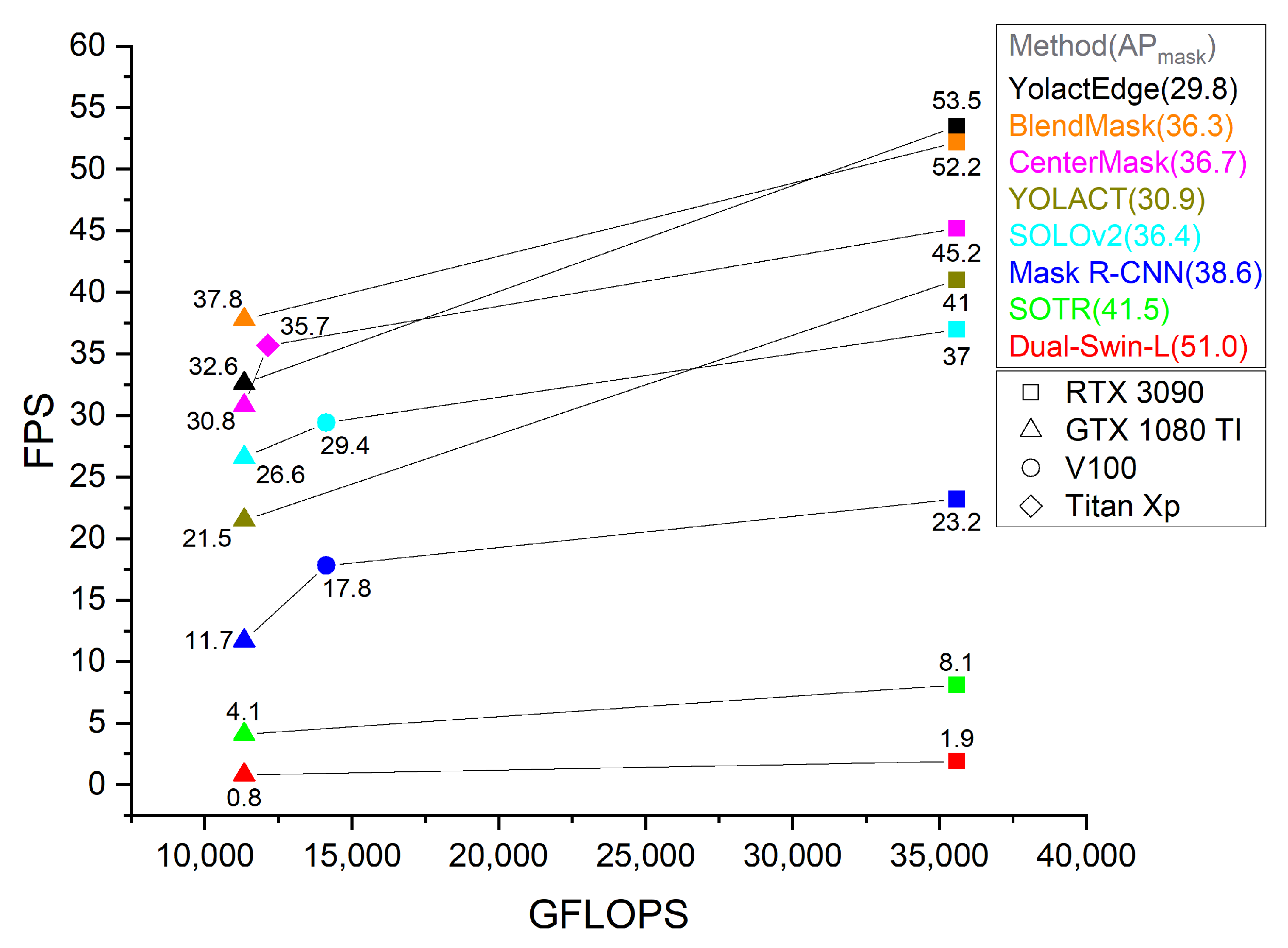
As shown in Table 2, the speed of the accuracy-focused models in the RTX 3090 environment was 1.9 FPS for Dual-Swin-L and 8.1 FPS for SOTR, both of which are slower than the 23.2 FPS result of Mask R-CNN. Additionally, in the GTX 1080 Ti environment, the speed was 0.8 FPS for Dual-win-L and 4.1 FPS for SOTR, whereas the speed of Mask R-CNN was estimated to be 11.7 FPS. The speeds of the speed-focused models in RTX 3090 environment were 53.5 FPS for YolactEdge, 52.2 FPS for BlendMask, 45.2 FPS for CenterMask, 41 FPS for YOLACT, and 37 FPS for SOLOv2, all of which were faster than the 23.2 FPS of Mask R-CNN. YolactEdge was estimated to run at 177.3 FPS when TensorRT optimization was applied. Additionally, in the GTX 1080 Ti environment, the speeds were 37.8 FPS for BlendMask, 32.6 FPS for YolactEdge, 30.8 FPS for CenterMask, 26.6 FPS for SOLOv2, and 21.5 FPS for YOLACT, all of which were faster than the 11.7 FPS of Mask R-CNN. YolactEdge was estimated to run at 81.6 FPS when TensorRT optimization was applied.
5.1.3. Accuracy Rate versus Inference Speed
As shown in Figure 17, the AP decreases as the FPS increases and vice versa in RTX 3090 and GTX 1080 Ti, respectively. This tendency is represented as an inversely proportional curve, so it can be confirmed that AP and FPS have a trade-off relationship.
5.1.4. RTX 3090 versus GTX 1080 Ti
5.1.5. GPU GFLOPS versus Inference Speed
5.2. Qualitative Results
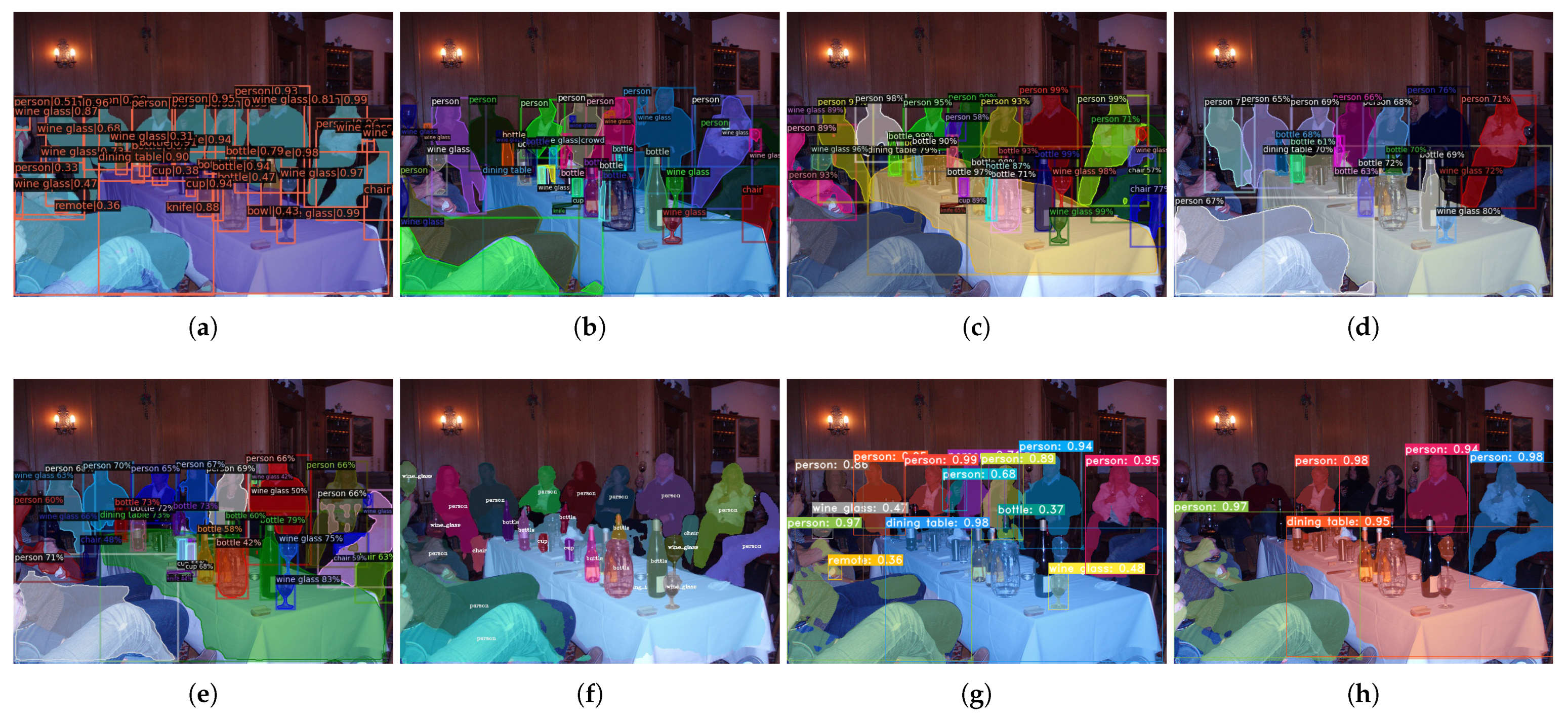
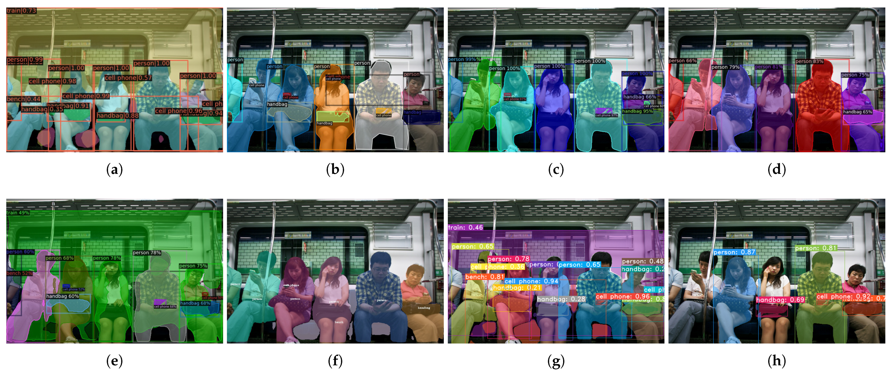
The segmentation performance results for human instances were similar, but YolactEdge performed worse than the other models, as shown in Figure 19, Figure 20 and Figure 21.
Figure 19 shows that, the accuracy-focused models segmented most of the objects on the central dining table. The speed-focused models segmented fewer objects on the dining table; however, CenterMask is the only model that recognized the knife on the dining table, and it obtained segmentation results that are similar to those of the accuracy-focused models. Among the speed-focused models, YOLACT recognized only one object on the dining table and YolactEdge did not recognize any.
Figure 20 shows that, Dual-Swin-L and CenterMask segmented the inner side of the subway train. All models except for BlendMask segmented at least one cell phone object held by people. It can be confirmed that the mask areas of different objects overlap in the Dual-Swin-L, CenterMask, and YOLACT results.
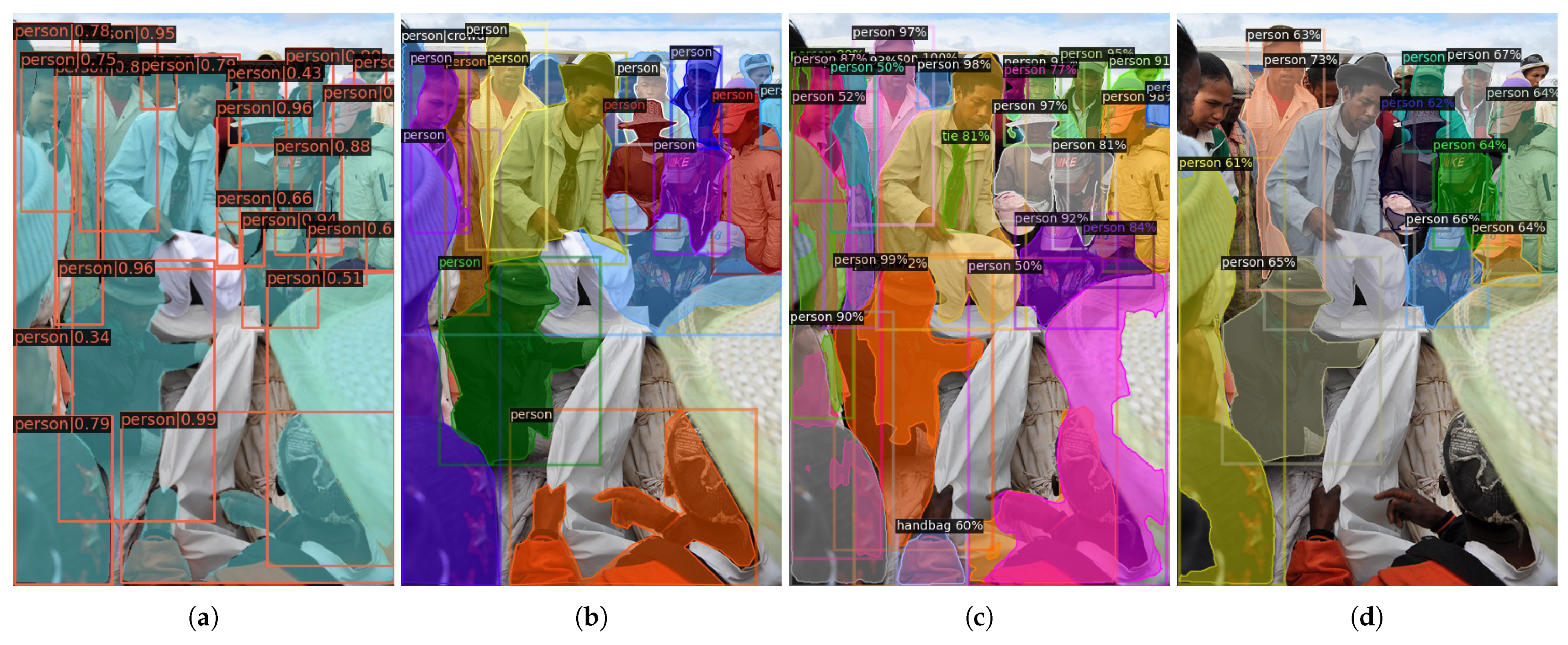
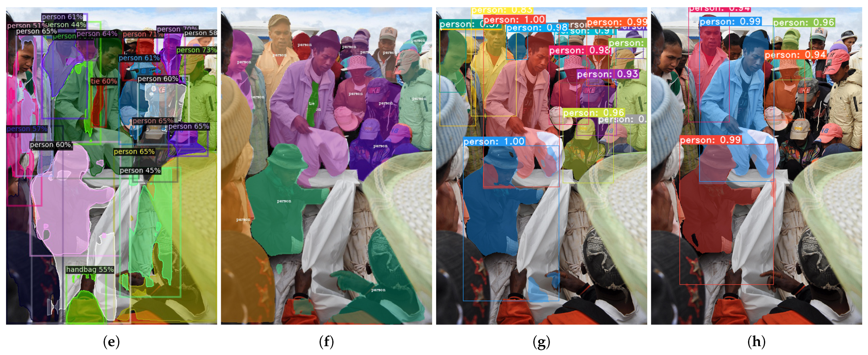
Figure 21 shows that, Mask R-CNN, CenterMask, and SOLOv2 segmented the necktie object from a human that was wearing one. Again, the mask regions of different objects overlap in the results of Mask R-CNN, CenterMask, YOLACT, and YolactEdge. In the results of CenterMask, YOLACT, and YolactEdge, there are empty spaces inside the mask regions and several disconnected mask areas.
6. Discussion
We categorized the experimental methods as accuracy-focused and speed-focused models, presented an overview of each model, and summarized their contribution. In addition, we ran an inference with MS COCO val2017 dataset [10] in a fixed test environment based on a GPU (RTX 3090 or GTX 1080 Ti) and compared the AP and FPS results of each model.
As shown in Table 1 and Figure 16a, the accuracy-focused models obtained relatively higher AP scores and relatively lower inference speed than the speed-focused models. Dual-Swin-L and SOTR outperformed Mask R-CNN in terms of AP. Furthermore, Dual-Swin-L has a noticeably higher AP than other models. We can infer from these results that the Transformer structure is an effective approach not only in the NLP field but also in computer vison. Although speed-focused models obtained lower AP scores than Mask R-CNN, all models run at real-time speed in the RTX 3090. Blendmask, Centermask, and YolactEdge also run at real-time speed in the GTX 1080 Ti, however, SOLOv2 and YOLACT do not run in real-time in the GTX 1080 Ti. In addition, we can confirm that AP and FPS have a trade-off relationship in Figure 17. Therefore, it seems that an appropriate trade-off between speed and accuracy should be considered for real-time use.
As stated above, speed-focused models have a faster inference speed than accuracy-focused models. Speed-focused models using the FPN structure have a speed of over 30 FPS in RTX 3090. Conversely, Dual-Swin-L [2] and SOTR [3], which use the Transformer structure, have a speed below 10 FPS. Mask R-CNN [4] was categorized as an accuracy-focused model, but because it uses an FPN structure, it has a relatively fast speed of 23.2 FPS in the RTX 3090 environment. Although they were not tested in this study, SipMask [52] and OrienMask [53], which can be categorized as speed-focused models, also used an FPN structure. OrienMask [53], which uses a Darknet-53 backbone, has reportedly achieved an AP of 34.5 and speed of 41.9 FPS on the COCO val2017 dataset in an RTX2080 Ti environment. SipMask [52], which uses a ResNet101-FPN backbone, has reportedly achieved an AP of 32.8 and speed of 31.2 FPS on the COCO test-dev dataset in a Titan Xp environment. Therefore, from the results on network structures released thus far, an FPN can be considered when designing a real-time model.
As shown in Table 2, when TensorRT optimization [22] was used for YolactEdge [9], the speed increased 2.5 times or more in the GTX 1080 Ti environment and 3.3 times or more in the RTX 3090 environment. However, no significant differences were observed in AP results. Therefore, we can expect a meaningful speed improvement by applying TensorRT to processing units that support CUDA. Furthermore, the recently unveiled NVIDIA Jetson AGX Orin [54] reportedly performed up to eight times faster than NVIDIA Jetson AGX Xavier [55]. Given that YOLACT achieved a 27.3 FPS in the NVIDIA Jetson AGX Xavier [39], high complexity models will be able to meet real-time requirements through TensorRT optimization in the NVIDIA Jetson product line, including the Jetson AGX Orin.
As shown in Table 1, different GPU environments lead to a difference in the inference speed but yield the same AP scores. Table 3 shows that comparison of the speeds of the methods in an RTX 3090 environment relative to that in a GTX 1080 Ti environment confirms that the improvements in speeds differ. Figure 18 also compares the GFLOPS and speed of each method. From these experimental results, we can confirm that the speed is proportional to the GFLOPS; however, the increase is not as significant.
Ignatov et al. [11] presented the performance of mobile SoCs in the fp-16 network and compared the performance of Intel CPUs and NVIDIA GPUs in the fp-32 network. The GPUs of mobile SoCs have a significant performance difference compared with workstation GPUs. Furthermore, even when the GPUs are the same, there is a difference in the performance depending on mobile SoCs. To explore the feasibility of using the comparison models in a mobile environment, we analyzed the correlation between workstation and mobile GPUs in Table 4, which shows the indicator of the comparative analysis including the GFLOPS of mobile chip and workstation GPUs. Although it is difficult to predict the mobile performance of the models we tested, it can provide some guidance for our future work. We will convert the models into mobile models to verify their performance.
7. Conclusions
Instance segmentation has gained attention in various areas of computer vision, leading to the development of many successful models. In this study, we tested and analyzed state-of-the-art instance segmentation models. We categorized the target methods as accuracy- and speed-focused models. We described the main contribution of each model and summarized its algorithm and method. We performed an inference experiment in a fixed environment with different GPUs to precisely compare and analyze these models and discussed the results obtained through quantitative and qualitative analyses. All speed-focused models run at real-time speed in the RTX 3090. Furthermore, Blendmask, Centermask, and YolactEdge also run at real-time speed in the GTX 1080 Ti, however, SOLOv2 and YOLACT do not run in real-time in the GTX 1080 Ti. Owing to the trade-off between speed and accuracy, a balance between them should be maintained for real-time use. Our experimental results show that using an FPN structure when designing a real-time model is a potential solution. In on-device AI, real-time use is crucial, making inference speed the most important factor. Although the performance of on-device AI chips is improving continuously, it is still inferior to that of workstation chips. Therefore, we investigated state-of-the-art models to understand the relationship between platforms and estimated the feasibility of on-device AI. However, it was difficult to predict the inference speed of on-device AI because of the lack of prior research. Therefore, we will convert and validate the model for on-device AI in future works; further, we will identify and analyze the factors affecting the inference speed of mobile.
Author Contributions
Conceptualization and methodology, S.J. and K.L.; software, S.J., H.H. and K.L.; validation, K.L., S.P. and S.-U.J.; writing—original draft, S.J., H.H. and K.L.; Writing—review and editing, S.J. and K.L. All authors have read and agreed to the published version of the manuscript.
Funding
This research was supported in part by the National Research Foundation of Korea (NRF) grant funded by the Korea government (MSIT) (No. 2020R1G1A1102041); by Electronics and Telecommunications Research Institute (ETRI) grant funded by ICT R&D program of MSIT/IITP (2021-0-00230, Development of real·virtual environmental analysis based adaptive interaction technology).
Conflicts of Interest
The authors declare no conflict of interest.
References
- Kirillov, A.; He, K.; Girshick, R.; Rother, C.; Dollár, P. Panoptic segmentation. In Proceedings of the IEEE/CVF Conference on Computer Vision and Pattern Recognition, Long Beach, CA, USA, 15–20 June 2019; pp. 9404–9413. [Google Scholar]
- Liang, T.; Chu, X.; Liu, Y.; Wang, Y.; Tang, Z.; Chu, W.; Chen, J.; Ling, H. Cbnetv2: A composite backbone network architecture for object detection. arXiv 2021, arXiv:2107.00420. [Google Scholar]
- Guo, R.; Niu, D.; Qu, L.; Li, Z. SOTR: Segmenting Objects with Transformers. In Proceedings of the IEEE/CVF International Conference on Computer Vision (ICCV), Montreal, QC, Canada, 10–17 October 2021; pp. 7157–7166. [Google Scholar]
- He, K.; Gkioxari, G.; Dollár, P.; Girshick, R. Mask r-cnn. In Proceedings of the IEEE International Conference on Computer Vision, Venice, Italy, 22–29 October 2017; pp. 2961–2969. [Google Scholar]
- Lee, Y.; Park, J. CenterMask: Real-Time Anchor-Free Instance Segmentation. In Proceedings of the IEEE/CVF Conference on Computer Vision and Pattern Recognition (CVPR), Seattle, WA, USA, 14–19 June 2020. [Google Scholar]
- Wang, X.; Zhang, R.; Kong, T.; Li, L.; Shen, C. Solov2: Dynamic and fast instance segmentation. Adv. Neural Inf. Process. Syst. 2020, 33, 17721–17732. [Google Scholar]
- Chen, H.; Sun, K.; Tian, Z.; Shen, C.; Huang, Y.; Yan, Y. Blendmask: Top-down meets bottom-up for instance segmentation. In Proceedings of the IEEE/CVF Conference on Computer Vision and Pattern Recognition, Seattle, WA, USA, 14–19 June 2020; pp. 8573–8581. [Google Scholar]
- Bolya, D.; Zhou, C.; Xiao, F.; Lee, Y.J. Yolact: Real-time instance segmentation. In Proceedings of the IEEE/CVF International Conference on Computer Vision, Seoul, Korea, 27 October–2 November 2019; pp. 9157–9166. [Google Scholar]
- Liu, H.; Soto, R.A.R.; Xiao, F.; Lee, Y.J. Yolactedge: Real-time instance segmentation on the edge. In Proceedings of the 2021 IEEE International Conference on Robotics and Automation (ICRA), Xi’an, China, 30 May–5 June 2021; pp. 9579–9585. [Google Scholar]
- Lin, T.Y.; Maire, M.; Belongie, S.; Hays, J.; Perona, P.; Ramanan, D.; Dollár, P.; Zitnick, C.L. Microsoft coco: Common objects in context. In Proceedings of the European Conference on Computer Vision, Zurich, Switzerland, 6–12 September 2014; Springer: Berlin/Heidelberg, Germany, 2014; pp. 740–755. [Google Scholar]
- Ignatov, A.; Timofte, R.; Kulik, A.; Yang, S.; Wang, K.; Baum, F.; Wu, M.; Xu, L.; Van Gool, L. Ai benchmark: All about deep learning on smartphones in 2019. In Proceedings of the 2019 IEEE/CVF International Conference on Computer Vision Workshop (ICCVW), Seoul, Korea, 27–28 October 2019; pp. 3617–3635. [Google Scholar]
- Luo, C.; He, X.; Zhan, J.; Wang, L.; Gao, W.; Dai, J. Comparison and Benchmarking of AI Models and Frameworks on Mobile Devices. arXiv 2020, arXiv:2005.05085. [Google Scholar]
- Bianco, S.; Cadene, R.; Celona, L.; Napoletano, P. Benchmark Analysis of Representative Deep Neural Network Architectures. IEEE Access 2018, 6, 64270–64277. [Google Scholar] [CrossRef]
- Huang, J.; Rathod, V.; Sun, C.; Zhu, M.; Korattikara, A.; Fathi, A.; Fischer, I.; Wojna, Z.; Song, Y.; Guadarrama, S.; et al. Speed/accuracy trade-offs for modern convolutional object detectors. In Proceedings of the IEEE Conference on Computer Vision and Pattern Recognition, Honolulu, HI, USA, 21–26 July 2017; pp. 7310–7311. [Google Scholar]
- Wang, Y.E.; Wei, G.Y.; Brooks, D. Benchmarking TPU, GPU, and CPU platforms for deep learning. arXiv 2019, arXiv:1907.10701. [Google Scholar]
- Ammirato, P.; Poirson, P.; Park, E.; Košecká, J.; Berg, A.C. A dataset for developing and benchmarking active vision. In Proceedings of the 2017 IEEE International Conference on Robotics and Automation (ICRA), Singapore, 29 May–3 June 2017; pp. 1378–1385. [Google Scholar]
- Perazzi, F.; Pont-Tuset, J.; McWilliams, B.; Van Gool, L.; Gross, M.; Sorkine-Hornung, A. A benchmark dataset and evaluation methodology for video object segmentation. In Proceedings of the IEEE Conference on Computer Vision and Pattern Recognition, Las Vegas, NV, USA, 27–30 June 2016; pp. 724–732. [Google Scholar]
- Lin, T.Y.; Dollár, P.; Girshick, R.; He, K.; Hariharan, B.; Belongie, S. Feature pyramid networks for object detection. In Proceedings of the IEEE Conference on Computer Vision and Pattern Recognition, Honolulu, HI, USA, 21–26 July 2017; pp. 2117–2125. [Google Scholar]
- Devlin, J.; Chang, M.W.; Lee, K.; Toutanova, K. Bert: Pre-training of deep bidirectional transformers for language understanding. arXiv 2018, arXiv:1810.04805. [Google Scholar]
- Vaswani, A.; Shazeer, N.; Parmar, N.; Uszkoreit, J.; Jones, L.; Gomez, A.N.; Kaiser, Ł.; Polosukhin, I. Attention is all you need. Adv. Neural Inf. Process. Syst. 2017, 30, 5999–6009. [Google Scholar]
- Dosovitskiy, A.; Beyer, L.; Kolesnikov, A.; Weissenborn, D.; Zhai, X.; Unterthiner, T.; Dehghani, M.; Minderer, M.; Heigold, G.; Gelly, S.; et al. An image is worth 16 × 16 words: Transformers for image recognition at scale. arXiv 2020, arXiv:2010.11929. [Google Scholar]
- Nvidia TensorRT. Available online: https://developer.nvidia.com/tensorrt (accessed on 14 July 2022).
- Ren, S.; He, K.; Girshick, R.; Sun, J. Faster r-cnn: Towards real-time object detection with region proposal networks. Adv. Neural Inf. Process. Syst. 2015, 28, 91–99. [Google Scholar] [CrossRef] [PubMed] [Green Version]
- Long, J.; Shelhamer, E.; Darrell, T. Fully Convolutional Networks for Semantic Segmentation. In Proceedings of the IEEE Conference on Computer Vision and Pattern Recognition (CVPR), Boston, MA, USA, 7–12 June 2015. [Google Scholar]
- Liu, Z.; Lin, Y.; Cao, Y.; Hu, H.; Wei, Y.; Zhang, Z.; Lin, S.; Guo, B. Swin transformer: Hierarchical vision transformer using shifted windows. In Proceedings of the IEEE/CVF International Conference on Computer Vision, Montreal, QC, Canada, 10–17 October 2021; pp. 10012–10022. [Google Scholar]
- Tian, Z.; Shen, C.; Chen, H.; He, T. FCOS: Fully Convolutional One-Stage Object Detection. In Proceedings of the IEEE/CVF International Conference on Computer Vision (ICCV), Seoul, Korea, 27 October–2 November 2019; pp. 9627–9636. [Google Scholar]
- Lin, T.Y.; Goyal, P.; Girshick, R.; He, K.; Dollár, P. Focal loss for dense object detection. In Proceedings of the IEEE International Conference on Computer Vision, Venice, Italy, 22–29 October 2017; pp. 2980–2988. [Google Scholar]
- Yang, L.; Fan, Y.; Xu, N. Video instance segmentation. In Proceedings of the IEEE/CVF International Conference on Computer Vision, Montreal, QC, Canada, 10–17 October 2019; pp. 5188–5197. [Google Scholar]
- Dosovitskiy, A.; Fischer, P.; Ilg, E.; Hausser, P.; Hazirbas, C.; Golkov, V.; Van Der Smagt, P.; Cremers, D.; Brox, T. Flownet: Learning optical flow with convolutional networks. In Proceedings of the IEEE International Conference on Computer Vision, Santiago, Chile, 7–13 December 2015; pp. 2758–2766. [Google Scholar]
- Wang, X.; Kong, T.; Shen, C.; Jiang, Y.; Li, L. Solo: Segmenting objects by locations. In Proceedings of the European Conference on Computer Vision, Glasgow, UK, 23–28 August 2020; Springer: Berlin/Heidelberg, Germany, 2020; pp. 649–665. [Google Scholar]
- Wu, Y.; Kirillov, A.; Massa, F.; Lo, W.Y.; Girshick, R. Detectron2. 2019. Available online: https://github.com/facebookresearch/detectron2 (accessed on 14 July 2022).
- Trained Model of DB-Swin-L. Available online: https://github.com/VDIGPKU/CBNetV2 (accessed on 14 July 2022).
- Trained Model of SOTR_R101_DCN. Available online: https://github.com/easton-cau/SOTR (accessed on 14 July 2022).
- Trained Model of R101-FPN. Available online: https://github.com/facebookresearch/detectron2/blob/main/MODEL_ZOO.md (accessed on 14 July 2022).
- Trained Model of centermask2-lite-V-39-eSE-FPN-ms-4x. Available online: https://github.com/youngwanLEE/centermask2 (accessed on 14 July 2022).
- Trained Model of SOLOv2_Light_512_DCN_R50_3x. Available online: https://github.com/WXinlong/SOLO (accessed on 14 July 2022).
- Trained Model of DLA_34_4x. Available online: https://github.com/aim-uofa/AdelaiDet/tree/master/configs/BlendMask (accessed on 14 July 2022).
- Trained Model of yolact_im700_54_800000. Available online: https://github.com/dbolya/yolact (accessed on 14 July 2022).
- Trained Model of yolact_edge_54_800000. Available online: https://github.com/haotian-liu/yolact_edge (accessed on 14 July 2022).
- Specifications of RTX 3090. Available online: https://www.nvidia.com/content/PDF/nvidia-ampere-ga-102-gpu-architecture-whitepaper-v2.pdf (accessed on 14 July 2022).
- GPU Clocks of Tesla V100. Available online: https://images.nvidia.com/content/tesla/pdf/Tesla-V100-PCIe-Product-Brief.pdf (accessed on 14 July 2022).
- CUDA Cores of Tesla V100. Available online: https://images.nvidia.com/content/technologies/volta/pdf/tesla-volta-v100-datasheet-letter-fnl-web.pdf (accessed on 14 July 2022).
- Specifications of RTX 2080, Ti. Available online: https://www.nvidia.com/en-me/geforce/graphics-cards/rtx-2080-ti/ (accessed on 14 July 2022).
- Specifications of Titan, Xp. Available online: https://www.nvidia.com/en-us/titan/titan-xp/ (accessed on 14 July 2022).
- Specifications of GTX 1080, Ti. Available online: https://www.nvidia.com/en-gb/geforce/graphics-cards/geforce-gtx-1080-ti/specifications/ (accessed on 14 July 2022).
- Specifications of HiSilicon Kirin 9000. Available online: https://www.cpu-monkey.com/en/cpu-hisilicon_kirin_9000 (accessed on 14 July 2022).
- Specifications of Snapdragon8 Gen 1. Available online: https://www.cpu-monkey.com/en/cpu-qualcomm_snapdragon_8_gen_1 (accessed on 14 July 2022).
- Specifications of Google Tensor. Available online: https://www.cpu-monkey.com/en/cpu-google_tensor (accessed on 14 July 2022).
- Specifications of Snapdragon 888. Available online: https://www.cpu-monkey.com/en/cpu-qualcomm_snapdragon_888 (accessed on 14 July 2022).
- Specifications of Snapdragon 870. Available online: https://www.cpu-monkey.com/en/cpu-qualcomm_snapdragon_870 (accessed on 14 July 2022).
- Specifications of Samsung Exynos 2100. Available online: https://www.cpu-monkey.com/en/cpu-samsung_exynos_2100 (accessed on 14 July 2022).
- Cao, J.; Anwer, R.M.; Cholakkal, H.; Khan, F.S.; Pang, Y.; Shao, L. Sipmask: Spatial information preservation for fast image and video instance segmentation. In Proceedings of the European Conference on Computer Vision, Glasgow, UK, 23–28 August 2020; Springer: Berlin/Heidelberg, Germany, 2020; pp. 1–18. [Google Scholar]
- Du, W.; Xiang, Z.; Chen, S.; Qiao, C.; Chen, Y.; Bai, T. Real-time Instance Segmentation with Discriminative Orientation Maps. In Proceedings of the IEEE/CVF International Conference on Computer Vision, Montreal, QC, Canada, 10–17 October 2021; pp. 7314–7323. [Google Scholar]
- Specifications of Jetson AGX Orin Developer Kit. Available online: https://developer.nvidia.com/embedded/jetson-agx-orin-developer-kit (accessed on 14 July 2022).
- Specifications of Jetson AGX Xavier Developer Kit. Available online: https://developer.nvidia.com/embedded/jetson-agx-xavier-developer-kit (accessed on 14 July 2022).
Figure 1.
Types of image segmentation. The mask results were graphically modified, not the actual inference results (COCO-val2017-000000116068 [10]).
Figure 1.
Types of image segmentation. The mask results were graphically modified, not the actual inference results (COCO-val2017-000000116068 [10]).

Figure 2.
Methods for extracting feature maps of various scales (COCO-val2017-000000007816 [10]).
Figure 2.
Methods for extracting feature maps of various scales (COCO-val2017-000000007816 [10]).

Figure 3.
Mask R-CNN architecture. The mask result was graphically modified, not the actual inference result (COCO-val2017-000000032901 [10]).
Figure 3.
Mask R-CNN architecture. The mask result was graphically modified, not the actual inference result (COCO-val2017-000000032901 [10]).

Figure 4.
SOTR architecture. “∗” indicates the dynamic convolution operation. The mask result was graphically modified, not the actual inference result (COCO-val2017-000000032861 [10]).
Figure 4.
SOTR architecture. “∗” indicates the dynamic convolution operation. The mask result was graphically modified, not the actual inference result (COCO-val2017-000000032861 [10]).

Figure 5.
Three transformer layer designs.

Figure 6.
Swin Transformer architecture.

Figure 7.
CBNetV2: dual-backbone architecture.

Figure 8.
Shifted window approach for computing self-attention (COCO-val2017-000000548267 [10]).
Figure 8.
Shifted window approach for computing self-attention (COCO-val2017-000000548267 [10]).

Figure 9.
CenterMask architecture. The box and mask results were graphically modified, not the actual inference result (COCO-val2017-000000015746 [10]).
Figure 9.
CenterMask architecture. The box and mask results were graphically modified, not the actual inference result (COCO-val2017-000000015746 [10]).

Figure 10.
YOLACT architecture. The mask result was graphically modified, not the actual inference result (COCO-val2017-000000021903 [10]).
Figure 10.
YOLACT architecture. The mask result was graphically modified, not the actual inference result (COCO-val2017-000000021903 [10]).

Figure 11.
YolactEdge architecture. The mask result was graphically modified, not the actual inference result (YouTube Video Instance Segmentation 2019 version-7a72130f21 [28]).
Figure 11.
YolactEdge architecture. The mask result was graphically modified, not the actual inference result (YouTube Video Instance Segmentation 2019 version-7a72130f21 [28]).

Figure 12.
Difference between FlowNetS [29] and FeatFlowNet [9] (YouTube Video Instance Segmentation 2019 version-7a72130f21 [28]).

Figure 13.
BlendMask architecture The mask result was graphically modified, not the actual inference result (COCO-val2017-000000561223 [10]).
Figure 13.
BlendMask architecture The mask result was graphically modified, not the actual inference result (COCO-val2017-000000561223 [10]).

Figure 14.
SOLO architecture. The mask result was graphically modified, not the actual inference result (COCO-val2017-000000079565 [10]).
Figure 14.
SOLO architecture. The mask result was graphically modified, not the actual inference result (COCO-val2017-000000079565 [10]).

Figure 15.
SOLOv2 mask branch. “∗” indicates the dynamic convolution operation. The mask result was graphically modified, not the actual inference result (COCO-val2017-000000079565 [10]).
Figure 15.
SOLOv2 mask branch. “∗” indicates the dynamic convolution operation. The mask result was graphically modified, not the actual inference result (COCO-val2017-000000079565 [10]).

Figure 16.
AP and FPS results for various instance segmentation methods on COCO-val2017: (a) RTX 3090 vs GTX 1080 Ti AP results for FPS; (b) AP and AP results on the RTX 3090 and GTX 1080Ti; (c) AP, AP results on the RTX 3090 and GTX 1080 Ti; (d) AP, AP results on the RTX 3090 and GTX 1080 Ti.
Figure 16.
AP and FPS results for various instance segmentation methods on COCO-val2017: (a) RTX 3090 vs GTX 1080 Ti AP results for FPS; (b) AP and AP results on the RTX 3090 and GTX 1080Ti; (c) AP, AP results on the RTX 3090 and GTX 1080 Ti; (d) AP, AP results on the RTX 3090 and GTX 1080 Ti.

Figure 17.
Speed–accuracy trade-off for various instance segmentation methods on COCO-val2017: (a) RTX 3090 speed–accuracy trade-off; (b) GTX 1080 Ti speed–accuracy trade-off.
Figure 17.
Speed–accuracy trade-off for various instance segmentation methods on COCO-val2017: (a) RTX 3090 speed–accuracy trade-off; (b) GTX 1080 Ti speed–accuracy trade-off.

Figure 18.
Comparison of GFLOPS according to speed for each inference GPU.

Figure 19.
Visualization of instance segmentation results (COCO-val2017-000000171190 [10]). (a) Dual-Swin-L; (b) SOTR; (c) Mask R-CNN; (d) BlendMask; (e) CenterMask; (f) SOLOv2; (g) YOLACT; (h) YolactEdge.
Figure 19.
Visualization of instance segmentation results (COCO-val2017-000000171190 [10]). (a) Dual-Swin-L; (b) SOTR; (c) Mask R-CNN; (d) BlendMask; (e) CenterMask; (f) SOLOv2; (g) YOLACT; (h) YolactEdge.

Figure 20.
Visualization of instance segmentation results (COCO-val2017-000000380913 [10]). (a) Dual-Swin-L; (b) SOTR; (c) Mask R-CNN; (d) BlendMask; (e) CenterMask; (f) SOLOv2; (g) YOLACT; (h) YolactEdge.
Figure 20.
Visualization of instance segmentation results (COCO-val2017-000000380913 [10]). (a) Dual-Swin-L; (b) SOTR; (c) Mask R-CNN; (d) BlendMask; (e) CenterMask; (f) SOLOv2; (g) YOLACT; (h) YolactEdge.

Figure 21.
Visualization of instance segmentation results (COCO-val2017-000000329323 [10]). (a) Dual-Swin-L; (b) SOTR; (c) Mask R-CNN; (d) BlendMask; (e) CenterMask; (f) SOLOv2; (g) YOLACT; (h) YolactEdge.
Figure 21.
Visualization of instance segmentation results (COCO-val2017-000000329323 [10]). (a) Dual-Swin-L; (b) SOTR; (c) Mask R-CNN; (d) BlendMask; (e) CenterMask; (f) SOLOv2; (g) YOLACT; (h) YolactEdge.


Table 1.
Benchmark results on MS COCO val2017 (-: when impossible to measure due to network structure; “*” indicates the FPS results with NVIDIA TensorRT optimization [22]).
Table 1.
Benchmark results on MS COCO val2017 (-: when impossible to measure due to network structure; “*” indicates the FPS results with NVIDIA TensorRT optimization [22]).
| Method | Model | Reference GPU | Tested GPU | Tested FPS | AP | AP | AP | AP | AP |
|---|---|---|---|---|---|---|---|---|---|
| Dual-Swin-L | DB-Swin-L [32] | NVIDIA V100 [2] | RTX 3090 | 1.9 | 51.0 | 59.1 | 32.2 | 54.3 | 69.0 |
| GTX 1080 Ti | 0.8 | ||||||||
| SOTR | SOTR_R101_DCN [33] | NVIDIA V100 [3] | RTX 3090 | 8.1 | 41.5 | - | 20.2 | 45.4 | 61.7 |
| GTX 1080 Ti | 4.1 | ||||||||
| Mask R-CNN | R101-FPN [34] | NVIDIA V100 (17.8 FPS) [34] | RTX 3090 | 23.2 | 38.6 | 42.9 | 19.4 | 41.3 | 55.3 |
| GTX 1080 Ti | 11.7 | ||||||||
| Centermask | centermask2-lite-V-39-eSE- FPN-ms-4x [35] | NVIDIA Titan Xp (35.7 FPS) [35] | RTX 3090 | 45.2 | 36.7 | 40.9 | 17.2 | 39.8 | 53.4 |
| GTX 1080 Ti | 30.8 | ||||||||
| SOLOv2 | SOLOv2_Light_512_DCN_ R50_3x [36] | NVIDIA V100 (29.4 FPS) [36] | RTX 3090 | 37.0 | 36.4 | - | 13.1 | 40.1 | 57.8 |
| GTX 1080 Ti | 26.6 | ||||||||
| Blendmask | DLA_34_4x [37] | GTX 1080 Ti (32.1 FPS) [37] | RTX 3090 | 52.2 | 36.3 | 40.8 | 16.0 | 39.6 | 53.9 |
| GTX 1080 Ti | 37.8 | ||||||||
| YOLACT | yolact_im700_54_800000 [38] | NVIDIA Titan Xp [8] | RTX 3090 | 41.0 | 30.9 | 33.4 | 12.0 | 34.3 | 48.9 |
| GTX 1080 Ti | 21.5 | ||||||||
| YolactEdge | yolact_edge_54_800000 [39] | RTX 2080 Ti [9] | RTX 3090 | 53.5/177.3 * | 29.8/29.9 * | 32.5/32.4 * | 10.1/9.9 * | 32.3/31.9 * | 50.2/50.4 * |
| GTX 1080 Ti | 32.6/81.6 * |
Table 2.
Frames per second on the RTX 3090 and GTX 1080 Ti. The SD and meidan are the standard deviation and the mean of two middle values, respectively (“*” indicates the FPS results with NVIDIA TensorRT optimization [22]).
Table 2.
Frames per second on the RTX 3090 and GTX 1080 Ti. The SD and meidan are the standard deviation and the mean of two middle values, respectively (“*” indicates the FPS results with NVIDIA TensorRT optimization [22]).
| Method | Tested GPU | Mean | SD | Min | Max | Median |
|---|---|---|---|---|---|---|
| YolactEdge | RTX 3090 | 53.5/177.3 * | 0.929/0.653 * | 51.9/176.2 * | 54.7/178.2 * | 53.9/177.5 * |
| GTX 1080TI | 32.6/81.6 * | 0.179/0.331 * | 32.4/80.8 * | 32.9/81.9 * | 32.6/81.8 * | |
| Blendmask | RTX 3090 | 52.2 | 0.231 | 51.9 | 52.6 | 52.2 |
| GTX 1080TI | 37.8 | 0.069 | 37.7 | 37.9 | 37.9 | |
| Centermask | RTX 3090 | 45.2 | 0.134 | 45.0 | 45.4 | 45.2 |
| GTX 1080TI | 30.8 | 0.035 | 30.8 | 30.9 | 30.8 | |
| YOLACT | RTX 3090 | 41.0 | 0.658 | 39.6 | 41.4 | 41.3 |
| GTX 1080TI | 21.5 | 0.205 | 21.1 | 21.7 | 21.6 | |
| SOLOv2 | RTX 3090 | 37.0 | 0.187 | 36.8 | 37.4 | 37.0 |
| GTX 1080TI | 26.6 | 0.064 | 26.5 | 26.7 | 26.6 | |
| Mask R-CNN | RTX 3090 | 23.2 | 0.024 | 23.1 | 23.2 | 23.2 |
| GTX 1080TI | 11.7 | 0.011 | 11.7 | 11.7 | 11.7 | |
| SOTR | RTX 3090 | 8.1 | 0.017 | 8.0 | 8.1 | 8.1 |
| GTX 1080TI | 4.1 | 0.008 | 4.1 | 4.2 | 4.1 | |
| Dual-Swin-L | RTX 3090 | 1.9 | 0.030 | 1.9 | 2.0 | 1.9 |
| GTX 1080TI | 0.8 | 0.030 | 0.7 | 0.8 | 0.8 |
Table 3.
MS COCO results on the RTX 3090 and GTX 1080 Ti. The relative performance on the RTX 3090 was quantified with respect to the FPS of the GTX 1080 Ti for each model (“*” indicates the FPS results with NVIDIA TensorRT [22] optimization).
Table 3.
MS COCO results on the RTX 3090 and GTX 1080 Ti. The relative performance on the RTX 3090 was quantified with respect to the FPS of the GTX 1080 Ti for each model (“*” indicates the FPS results with NVIDIA TensorRT [22] optimization).
| Method | Tested GPU | Tested FPS | Relative Performance (%) RTX 3090/GTX 1080 Ti |
|---|---|---|---|
| YolactEdge | RTX 3090 | 53.5/177.3 * | 164/217 * |
| GTX 1080 Ti | 32.6/81.6 * | ||
| Blendmask | RTX 3090 | 52.2 | 138 |
| GTX 1080 Ti | 37.8 | ||
| Centermask | RTX 3090 | 45.2 | 147 |
| GTX 1080 Ti | 30.8 | ||
| YOLACT | RTX 3090 | 41 | 191 |
| GTX 1080 Ti | 21.5 | ||
| SOLOv2 | RTX 3090 | 37 | 139 |
| GTX 1080 Ti | 26.6 | ||
| Mask R-CNN | RTX 3090 | 23.2 | 198 |
| GTX 1080 Ti | 11.7 | ||
| SOTR | RTX 3090 | 8.1 | 198 |
| GTX 1080 Ti | 4.1 | ||
| Dual-Swin-L | RTX 3090 | 1.9 | 238 |
| GTX 1080 Ti | 0.8 |
Table 4.
Comparison of the GFLOPS of recent workstation GPU and mobile SoCs. The GPU clock is based on the boost clock; the GFLOPS calculation of the workstation GPU is as follows: GPU clock × cores × 2 (operation/cycle); the relative GFLOPS of the workstation and mobile GPUs are presented relative to the performance of the GTX 1080 Ti.
| Device | GPU Clock (GHz) | GFLOPS (FP32) | Relative GFLOPS (%) |
|---|---|---|---|
| RTX 3090 [40] | 1695 | 35,581 | 313.7 |
| Tesla V100 [41,42] | 1380 | 14,131 | 124.6 |
| RTX 2080 Ti [43] | 1545 | 13,447 | 118.5 |
| Titan Xp [44] | 1582 | 12,149 | 107.1 |
| GTX 1080 Ti [45] | 1582 | 11,339 | 100 |
| HiSilicon Kirin 9000 [46] (ARM Mali-G78 MP24) | 760 | 2332 | 20.5 |
| Snapdragon8 gen 1 [47] (Qualcomm Adreno 730) | 820 | 2236 | 19.7 |
| Google Tensor [48] (ARM Mali-G78 MP20) | 760 | 1943 | 17.1 |
| Snapdragon 888 [49] (Qualcomm Adreno 660) | 840 | 1720 | 15.1 |
| Snapdragon 870 [50] (Qualcomm Adreno 650) | 670 | 1418 | 12.5 |
| Samsung Exynos 2100 [51] (ARM Mali-G78 MP14) | 760 | 1360 | 11.9 |
Publisher’s Note: MDPI stays neutral with regard to jurisdictional claims in published maps and institutional affiliations. |
© 2022 by the authors. Licensee MDPI, Basel, Switzerland. This article is an open access article distributed under the terms and conditions of the Creative Commons Attribution (CC BY) license (https://creativecommons.org/licenses/by/4.0/).
Share and Cite
MDPI and ACS Style
Jung, S.; Heo, H.; Park, S.; Jung, S.-U.; Lee, K. Benchmarking Deep Learning Models for Instance Segmentation. Appl. Sci. 2022, 12, 8856. https://0-doi-org.brum.beds.ac.uk/10.3390/app12178856
AMA Style
Jung S, Heo H, Park S, Jung S-U, Lee K. Benchmarking Deep Learning Models for Instance Segmentation. Applied Sciences. 2022; 12(17):8856. https://0-doi-org.brum.beds.ac.uk/10.3390/app12178856
Chicago/Turabian StyleJung, Sunguk, Hyeonbeom Heo, Sangheon Park, Sung-Uk Jung, and Kyungjae Lee. 2022. "Benchmarking Deep Learning Models for Instance Segmentation" Applied Sciences 12, no. 17: 8856. https://0-doi-org.brum.beds.ac.uk/10.3390/app12178856
Note that from the first issue of 2016, this journal uses article numbers instead of page numbers. See further details here.