
Shear Wave Velocity Estimation Based on Deep-Q Network

Department of Electronic Systems, Norwegian University of Science and Technology, 7491 Trondheim, Norway
*
Author to whom correspondence should be addressed.
Appl. Sci. 2022, 12(17), 8919; https://0-doi-org.brum.beds.ac.uk/10.3390/app12178919
Submission received: 28 June 2022
/
Revised: 29 August 2022
/
Accepted: 1 September 2022
/
Published: 5 September 2022
(This article belongs to the Special Issue Advances in Artificial Intelligence: Machine Learning, Data Mining and Data Sciences)
Abstract
:Geoacoustic inversion is important for seabed geotechnical applications. It can be formulated as a problem that seeks an optimal solution in a high-dimensional parameter space. The conventional inversion approach exploits optimization methods with a pre-defined search strategy whose hyperparameters need to be fine-tuned for a specific scenario. A framework based on the deep-Q network is proposed in this paper and the environment and agent configurations of the framework are specially defined for geoacoustic inversion. Unlike a conventional optimization method with a pre-defined search strategy, the proposed framework determines a flexible strategy by trial and error. The proposed framework is evaluated by two case studies for estimating the shear wave velocity profile. Its performance is compared with three global optimization methods commonly used in underwater geoacoustic inversion. The results demonstrate that the proposed framework performs the inversion more efficiently and accurately.
1. Introduction
Shear wave velocity estimation is an important geoacoustic inversion task for seabed geotechnical applications since shear wave velocity can provide a good indicator of sediment rigidity and characterization [1,2]. The seabed shear wave velocity profile can be estimated from the dispersion curve of the seismoacoustic interface waves, which is a convenient and low-cost approach compared to the direct approach (e.g., coring). Here, the interface waves refer to Scholte waves since in most underwater and seismic experiments sources are deployed in the water column and only Scholte waves can be generated [2].
There are two approaches for geoacoustic inversion [3]: the optimization-based approach and the machine learning (ML)-based approach. The optimization-based approach exploits the optimization method for determining a set of geoacoustic parameters that best fit the measured data. Based on the previous reviews [4,5], some optimization methods have been demonstrated to perform well for geoacoustic inversions, such as the genetic algorithm (GA) [6], differential evolution (DE) [7], and adaptive simplex simulated annealing (ASSA) [8]. On the other hand, with the development of ML, studies for geoacoustic inversion based on ML have appeared. Most of the studies are based on supervised learning, which aims to train a deep neural network for inversion based on a vast dataset [9,10,11,12]. This type of approach normally consists of the following steps: (1) creating a simulation dataset based on a physical forward model; (2) training a deep neural network based on the simulation dataset; (3) exploiting the trained neural network for the real-world inversion.
These two approaches can both provide acceptable performances for geoacoustic inversion. However, they also have some drawbacks. Since the prevalent optimization methods are not specifically designed for geoacoustic inversion, they may incur some limitations and difficulties to be applied in this specific field, such as difficulties in choosing the hyperparameters required by the algorithm, which may incur more time–costs. The ML-based approach introduces a drawback that the trained neural network cannot interact with the physical forward model. The procedure of creating the simulation dataset has to be repeated when the ocean environment changes significantly.
To avoid the drawbacks and keep the interactive ability of the optimization-based approach and the learnability of the ML-based approach, deep reinforcement learning (DRL) could become a potential option. Unlike supervised learning, DRL learns by trial and error, which iteratively updates the model by interacting with the environment to achieve good data fitting [13]. Its potential for geoacoustic inversion can be intuitively interpreted. The physical forward model role, e.g., the environment, can create a replica according to a set of geoacoustic parameters input by the DRL model. The DRL method can update the model by iteratively modifying the replica to obtain the best fit of the measured data.
DRL has been widely used as an intelligent controller for different purposes, including robotics [14], electronic sports [15], automatic controlling [16,17,18,19,20,21,22,23], etc. Specifically, Gu et al. demonstrated the effectiveness of DRL for controlling physical robots [14]. Joo et al. proposed a green signal time allocation system based on a deep Q-network (DQN) for reducing the standard deviation of each lane at an intersection [16]. Zhou et al. modeled penetration testing as a Markov decision process and exploited DQN for autonomous penetration testing [17]. Park et al. exploited a DRL-based DQN agent for a visual object-tracking task in a virtual environment. It has been demonstrated that the proposed agent outperforms some conventional methods of two public databases [18]. Gao et al. proposed a DRL-based method to solve the relay selection problem in the decode and forward relay-aided free-space optical communication system [19]. Guan et al. designed a DRL-based spectrum allocation algorithm for the internet of vehicles discriminating services. It has been proven that the designed method allocates spectrum resources quickly and efficiently in a highly dynamic environment [20]. Zhao et al. utilized DQN for controlling the autonomous walking of an underground load–haul–dump machine and demonstrated the effectiveness of the proposed DQN-based method through experimental verification [21]. Qin et al. proposed a hierarchical DQN-based path-planning method for controlling the long-term data collection of unmanned aerial vehicles in dynamic scenarios [22]. Asaf et al. exploited DRL to set optimal contention windows under different network conditions for wireless LAN performance enhancement [23].
Even though it has been illustrated that the DRL outperforms to control the agent’s behavior for performing well in a specific environment, the application of DRL still needs a specific configuration of the environment, action space of the agent, and reward. For instance, Wang et al. proposed a stochastic inversion of magnetotelluric data based on DRL [24], in which the environment state is defined as the layer information and the resistivity, and the agent space includes three linear operations (addition, subtraction, and keeping no variation). However, the problem of magnetotelluric inversion is quite different from the geoacoustic inversion. Moreover, the parameter space of the latter is a high-dimensional space, which means that the naive linear operations (e.g., addition or subtraction) are inefficient for the agent to explore in the space and determine the optimal solution. To the best of our knowledge, DRL has not been used for geoacoustic inversion. Therefore, our motivation is to investigate the potential of DRL and define a useful configuration of the environment and agent for the field.
In this paper, we propose a geoacoustic inversion framework based on a popular method of DRL and the DQN for estimating shear wave velocity from the dispersion data of interface waves. In the framework, a carefully designed configuration for the environment and agent is also proposed. A comprehensive performance analysis is presented to compare the proposed framework with three popular optimization methods (i.e., GA, DE, and ASSA) widely used for geoacoustic inversion.
The remainder of this paper is organized as follows. Section 2 states the considered problem. The theories of DRL and DQN are introduced in Section 3. Section 4 describes the proposed framework for geoacoustic inversion. A comprehensive performance analysis is presented in Section 5. Finally, the conclusions are given in Section 6.
2. Problem Formulation
The definition of the forward problem can be expressed as
where F and refer to the physical forward model and the observed data, respectively. is a set of geoacoustic parameters standing for one ocean environment and seabed condition.
The inversion problem aims at inferring the set of geoacoustic model parameters generating the observed data and can be expressed as:
where refers to the inversion operation.
The ocean environment and seabed can be parameterized as an N-layered structure with four geoacoustic parameters (layer thickness, density, compression wave velocity, and shear wave velocity): .
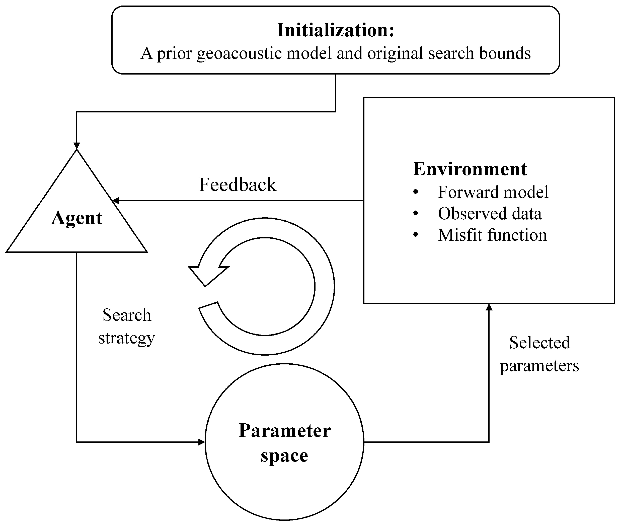
A general workflow of inversion is illustrated in Figure 1. The terminologies are introduced as follows:
- The environment consists of a physical forward model for calculating the replica, the observed data, and a misfit function for measuring the mismatch between the observed data and the replica. It receives a set of selected parameters from the agent and provides feedback to the agent.
- An agent is an operator that samples from the parameter space following its search strategy and interacts with the environment. During each iteration of inversion, the agent will log the feedback from the environment, the instant best solution, and the related information.
- A parameter space is a multi-dimensional space defined by the search bounds.
The inversion is an iterative process. It starts with an initialization that defines a prior geoacoustic model and the original search bounds based on prior knowledge. During each iteration, the agent will sample from the parameter space. The environment will receive the selected parameters, correspondingly create a replica, and provide the misfit as feedback for the agent. The iteration stops once the termination criteria are met.
As shown in Figure 1, the existing optimization methods (GA, DE, and ASSA) role as the search strategy for controlling the agent to explore the parameter space and determine the best solution at the end. Specifically, GA [6] and DE [7] are two heuristic search algorithms inspired by the evolution of natural species. ASSA [8] is a hybrid optimization method that combines the downhill simplex and the simulated annealing methods. More details about GA, DE, and ASSA can be found in [6,7,8], respectively.
3. Theories of DRL and DQN
DRL is used to solve a type of task that controls an agent to iteratively interact with the environment, and maximize future rewards. This task can be formulated as a finite Markov decision process [25] and be achieved by the DQN algorithm [13]. DQN is derived from Q-learning and can learn an optimal strategy by estimating the Q-value, which expresses the quality of executing an action a given a certain environment state s. The Q-value can be iteratively updated by the following formula and converge to the optimum.
where expresses the Q-value at the current environment state, is the learning rate, r is the current reward, is the discount factor, and represents the maximum Q-value in the next environment state .
The conventional Q-learning needs to create a Q-table for saving and updating the Q-value at each environment state, which can be intractable to build a table when the environment state number is huge. To mitigate this problem, the DQN algorithm utilizes a neural network instead of a Q-table for estimating the Q-value. The DQN algorithm introduces a replay memory to save the agent’s experience at different iterations, where is the experience at t iteration. During the training stage, the DQN randomly selects a mini-batch from the replay memory for minimizing a loss function L:
where the meanings of symbols are the same as in Equation (3).
Given a specific configuration of the environment and agent, the training process of DQN is expressed in Algorithm 1 [13].
| Algorithm 1: Training procedure of DQN |
|
4. Geoacoustic Inversion Framework Based on DQN
In this section, the DQN-based framework for geoacoustic inversion is presented from the DRL perspective (namely, the DQN framework).
4.1. Environment Configuration
As shown in Figure 1, the environment intakes the selected parameters and provides feedback for the agent to update the search results. During each iteration, the agent inputs k sets of selected parameters and the environment provides feedback to the agent.
The configuration of the environment for the DQN framework is listed as follows:
- The physical forward model: a theoretical program for calculating the replica.
- Observed data: the measured data or the data derived from the measured data.
- Misfit function: the root mean squared error (RMSE) measures the difference between the observed data and replica.
- Environment state: a special item for the DQN framework, which indicates the progress of the inversion. The environment state is formulated as:where i refers to the ith iteration, , , and are operators for calculating minimum, mean, and standard deviation, respectively. refers to the normalized misfit values corresponding to k sets of parameters, where is the minimum misfit value in the initialization stage and acts as the normalization factor. is an operator for calculating the difference from the last iteration, e.g., .
- Termination criteria: whenever one of the conditions expressed below is satisfied, the iteration stops.where is the maximum iterations, is a preset threshold of misfit, and is a preset threshold for convergence.
- Reward: a special item for the DQN framework, which is a signal for guiding the agent to learn a search strategy. For obtaining a fast and accurate search strategy, the reward rules are defined as:
- Feedback: the feedback includes misfit values , the environment state and the reward.
4.2. Agent and Action Space
Action space consists of all the potential actions that may be selected by the agent during each iteration. For instance, the action space of GA consists of reproduction, crossover, and mutation [6]. The configuration of the agent for the DQN framework is listed as follows:
- Agent state: during each iteration, the agent updates the agent state based on the feedback from the environment. The agent state is formulated aswhere refers to the search bounds of the parameters, is a set of parameters with the lowest misfit value among the k-selected sets. and are mean and standard deviation values of the parameters, respectively, whose misfit values are the first 30% lowest values among the k-selected sets.
- Action space: the agent has two actions for sampling from the parameter space. Each action consists of a sampling operation and an update rule.
- –
- Action 0 samples with the uniform distribution from the search bounds and iteratively searches the solution by compressing .More specifically, during each iteration, the agent conducts two steps:
- At beginning of the ith iteration, the search bounds are compressed as follows:
- After updating the search bounds, k sets of parameters are sampled with a uniform distribution from the updated search bounds . The selected parameters are fed into the environment and the corresponding feedback is received by the agent. The agent state is updated accordingly.
- –
- Action 1 samples with the Gaussian distribution and iteratively searches the solution by updating and of the selected k sets.More specifically, during each iteration, the agent conducts the following steps:
- At the beginning of the ith iteration, k sets of parameters are sampled with a Gaussian distribution defined by . Note that the operation of sampling needs to be repeated when any of the selected parameters exceed the original search bounds or the bounds of , where the subscripts and refer to the lower and upper bounds of , respectively.
- The selected parameters are fed into the environment and the corresponding feedback is received by the agent. The agent state, except for the search bounds , will be updated accordingly.
- In the received feedback, if , the expansion is activated for jumping out of the local minimum. The expansion is conducted as follows:
- (a)
- = 10
- (b)
- (c)
- Repeating steps 1 and 2.
4.3. DQN-Based Search Strategy
The search strategy acts as a guide that leads the agent to iteratively select an action from the action space according to the feedback from the environment. For instance, the search strategy of GA consists of a series of pre-defined rules that leads the agent of GA to find the optimal solution.
Unlike the existing optimization methods, which have a pre-defined search strategy, the DQN framework learns the strategy for controlling the agent defined in Section 4.2 by iteratively interacting with the environment defined in Section 4.1 to find a set of parameters corresponding to the lowest misfit value as quickly as possible.
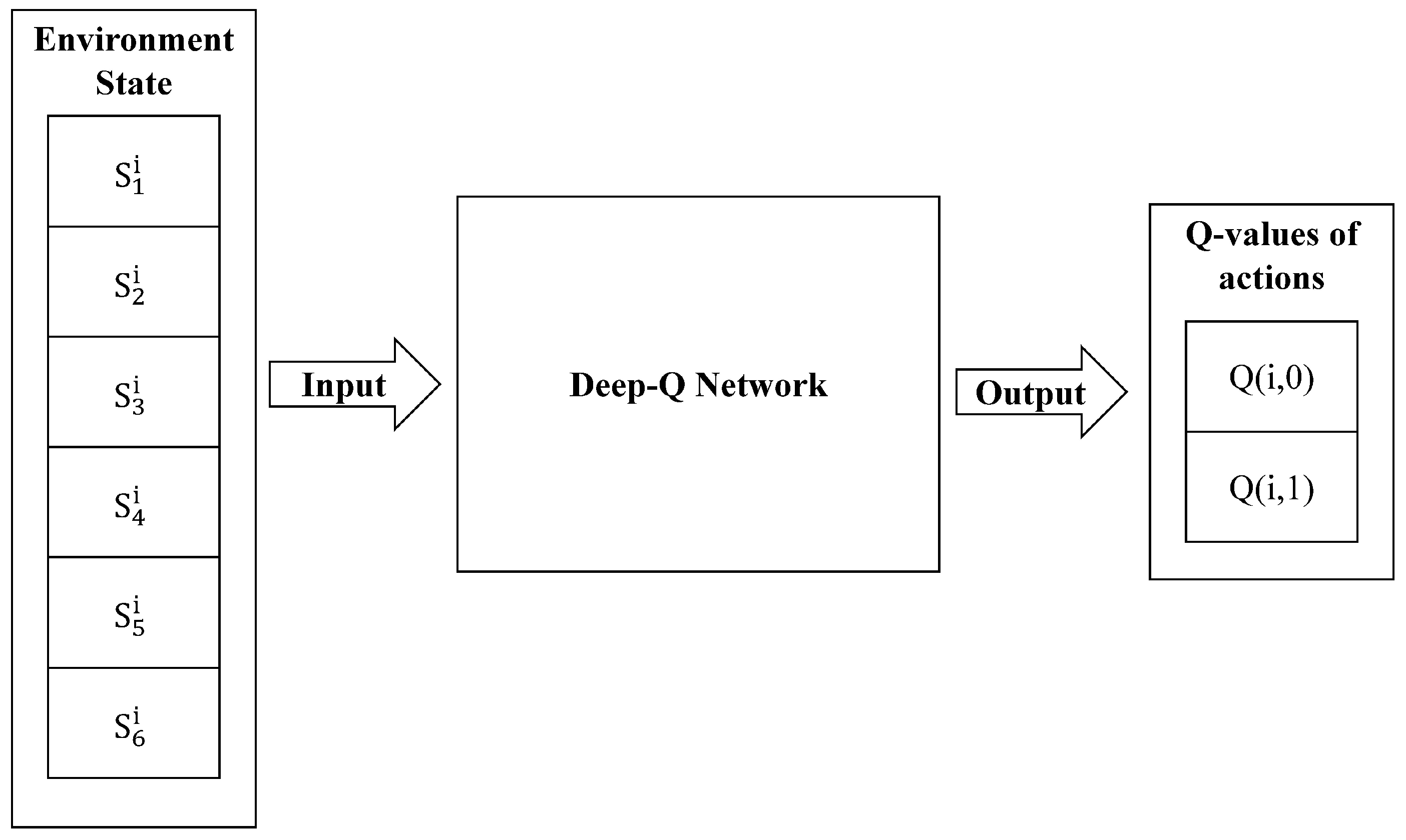
The DQN-based search strategy is shown in Figure 2, where the architecture of the neural network is expressed in Table 1. The neural network has three dense layers followed by the ReLU activation function with the exception of dense layer 3. The input for dense layer 1 is the current environment state , a vector consisting of six components. The output by dense layer 3 is a two-component vector expressing the Q-values corresponding to the possibilities of executing actions, and the agent will execute the action with a larger Q-value.
4.4. Inversion Workflow
The inversion workflow based on the DQN framework is expressed in Algorithm 2:
| Algorithm 2: Inversion workflow based on the DQN framework. |
|
In the initialized environment state , , , and are the minimum, mean, and standard deviations of the misfit values (with a dimension that depends on the inverse problem) among the k selected sets. Specifically, involves the normalization factor, and each item of the environment state is a percentage.
4.5. Implementation
Upon the environment and agent defined in Section 4.1 and Section 4.2, the DQN framework is trained following the procedure in Section 3.
Hyperparameters of the implementation are shown in Table 2.
5. Numerical Experiments
In this paper, the DQN framework is applied to estimate the shear wave velocity based on the dispersion data of interface waves. The inversion performances of the proposed DQN framework and three alternative methods (GA, DE, and ASSA) are examined in two numerical experiments. Two geoacoustic models based on real scenarios in [2,26] are defined to increase the reality of the simulation. To increase the reliability of the evaluation, the inversion results discussed in this section are averaged over 100 independent inversions. A forward model DISPER80 [27] based on the Thomson–Haskell matrix method [28,29] is used for calculating the simulated dispersion curve based on the given geoacoustic model.
5.1. Experiment Setup
The numerical experiments were conducted on a server with Intel Core i7-9700K CPU @ 3.60 GHz, 8 cores, 64 G memory, and 1 T hard drive. Inversions of GA and DE were implemented based on a GitHub repository scikit-opt. The inversion of ASSA was implemented based on the algorithm proposed in [8]. The DQN framework was implemented based on PyTorch [30]. Preset parameters of the candidate methods are shown in Table 3, where item All refers to the parameters applicable for all the candidate methods.
The metrics for evaluation are the misfit value, the running time per independent inversion and the relative error (namely, RE) formulated in Equation (11).
where is the estimated value of one geoacoustic parameter and is the corresponding ground truth.
5.2. Case 1
Case 1 defines a six-layer geoacoustic model referenced from the inversion results in the Grane field [26], as shown in Table 4. The phase velocity dispersion curves for the first five modes of the Scholte waves are calculated in the frequency range from 0 to 5 Hz as the ground truth.
The density and compression wave velocities are considered as known since they are not sensitive to the dispersion property of the Scholte wave [1]. The original search bounds for Case 1 are shown in Table 5.
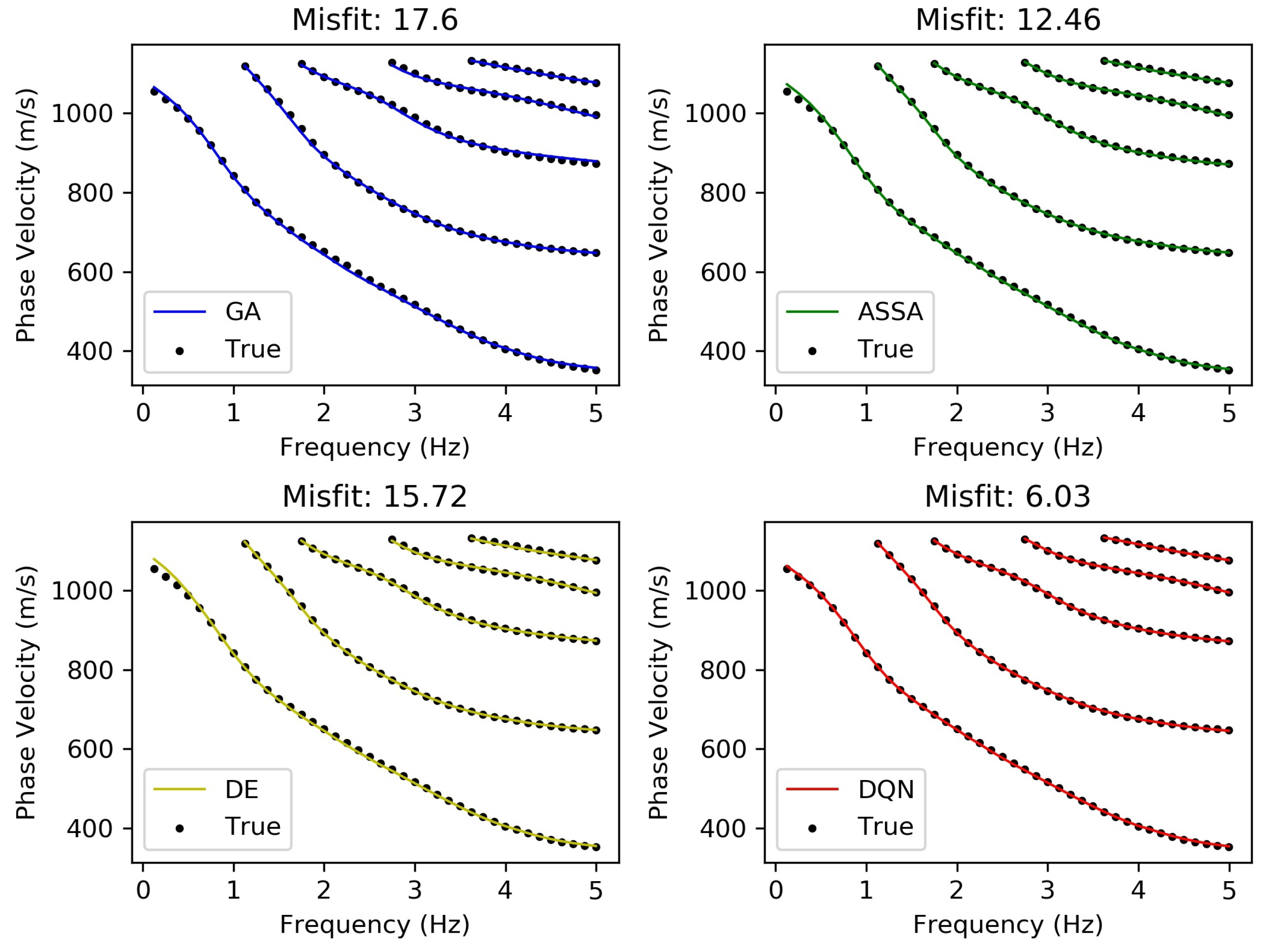
The estimated dispersion curves with the ground truth are shown in Figure 3, where the black dots are the ground truth. The blue, green, yellow, and red lines express the estimated dispersion curves by the GA, ASSA, DE, and DQN framework, respectively.
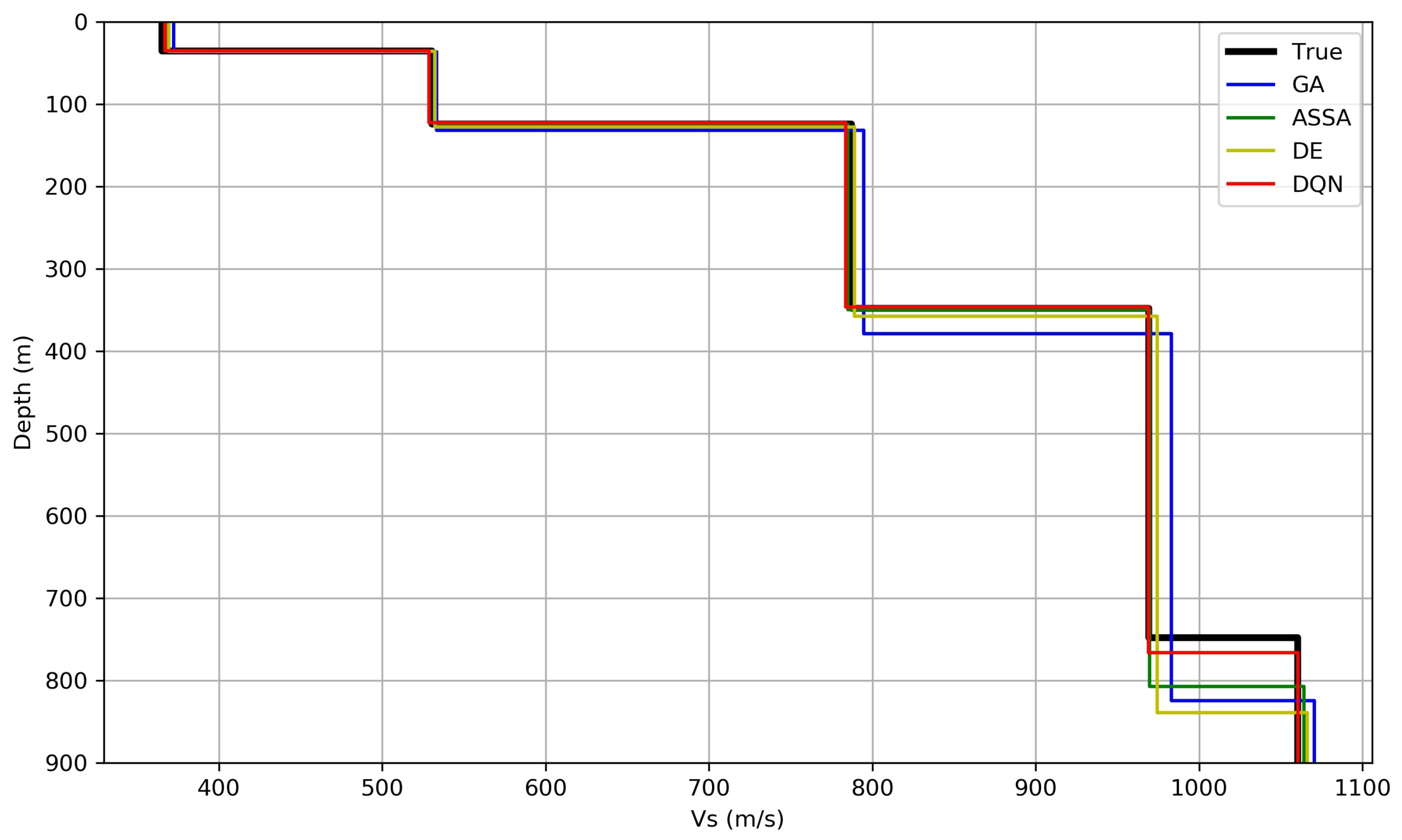
The estimated shear wave velocity profiles with the ground truth are shown in Figure 4, where the black line refers to the ground truth. The blue, green, yellow, and red lines express the estimated shear wave velocity profiles by the GA, ASSA, DE, and DQN framework, respectively.
The performance analysis for Case 1 is shown in Table 6, in which the bold fonts refer to the lowest relative error, misfit value, or running time over each row.
- At the low frequency of the fundamental mode, the estimated errors by ASSA and DE are larger than that by the GA and DQN framework.
- For all candidate methods, the relative errors of the shear wave velocity in all layers are lower than that of thickness. Both the shear wave velocity and layer thickness are sensitive to the dispersion properties of Scholte waves. However, in some cases, one can be more sensitive than the other.
- The low-to-high ranking for misfit values is the DQN framework, ASSA, DE, and GA. It is the same as the low-to-high ranking for the relative error of each geoacoustic parameter with a few exceptions of , , , and . This illustrates that the misfit value has a partly positive correlation with the overall relative errors, which is significant since the ground truth of a field survey is mostly unknown and the misfit value is the only metric.
- The DQN framework attains the lowest misfit and the shortest running time over others. Furthermore, the DQN framework has the lowest relative errors of all estimated geoacoustic parameters with a few exceptions of and .
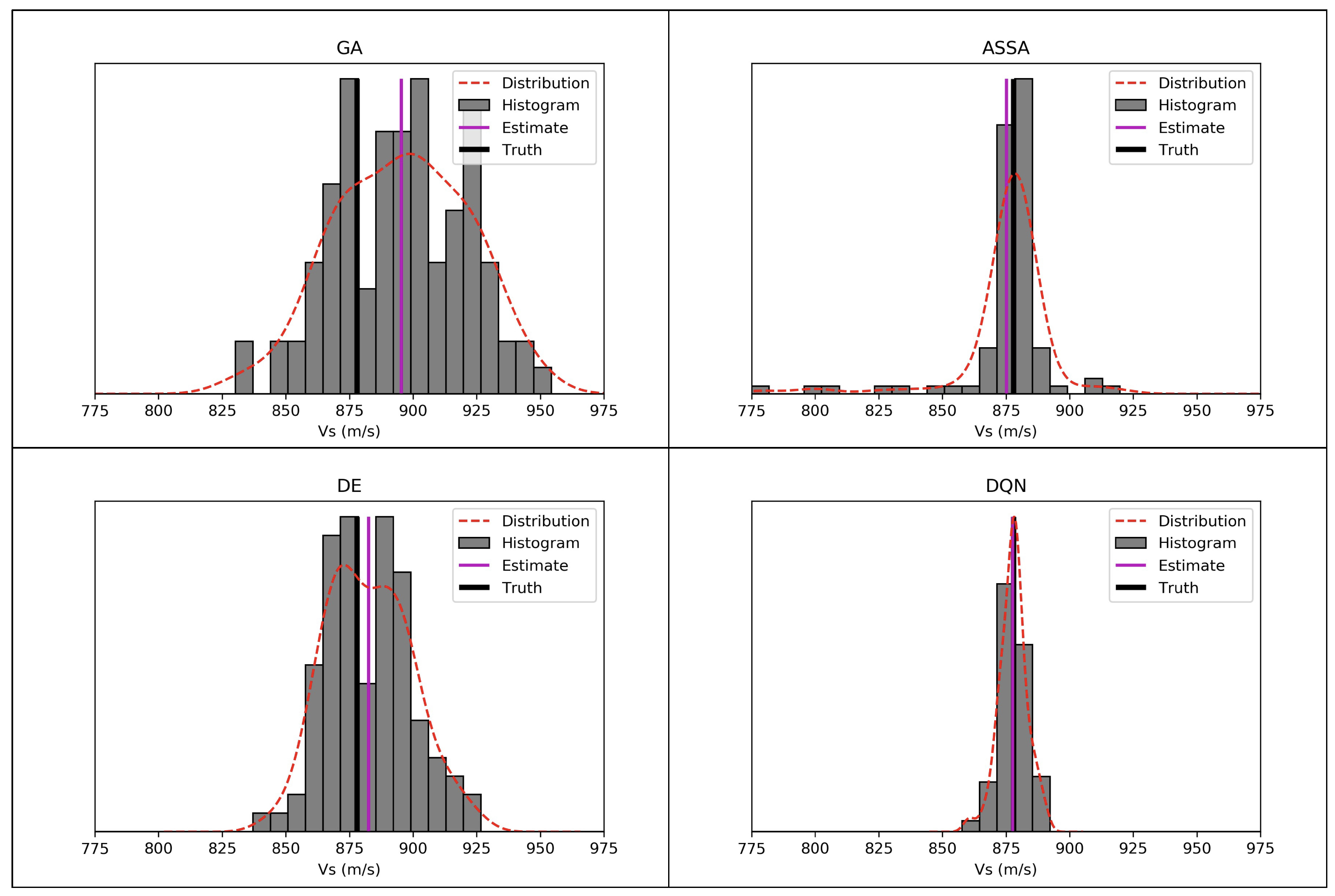
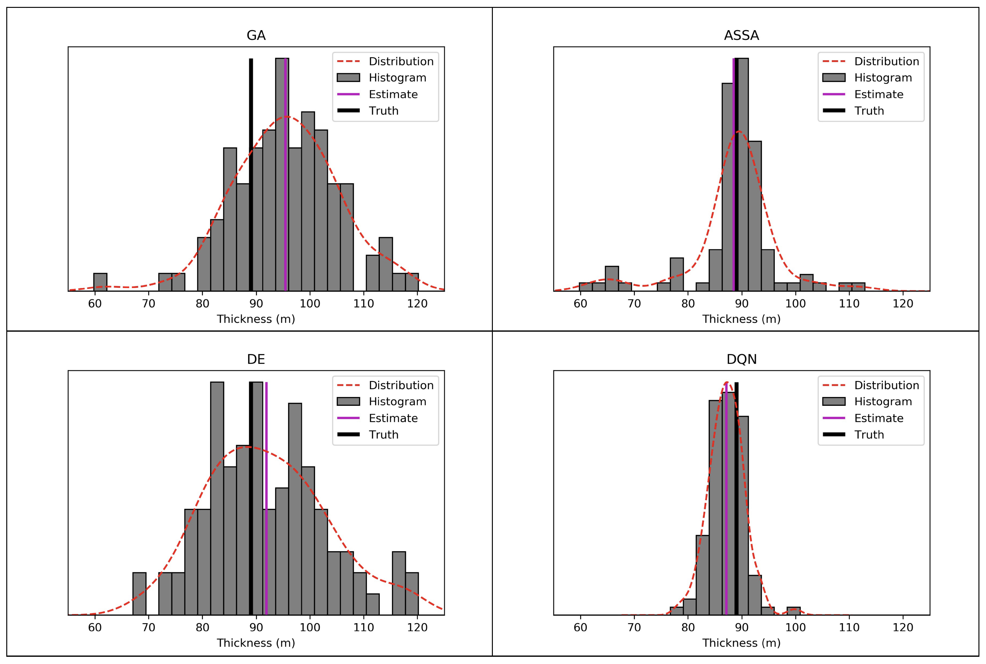
Two geoacoustic parameters are picked for further statistical analysis since the DQN framework performs the best inversion on and does not perform the best on . The statistical analyses of geoacoustic parameters and are shown in Figure 5 and Figure 6, respectively. In the figures, the red dashed curve illustrates the distribution of the estimated parameter over 100 independent inversions. The gray block, the purple line, and the black line correspond to the histogram, averaged value over 100 independent inversions, and the ground truth, respectively. Intuitively, the closeness between the purple and black lines indicates the inversion performance (the closer, the better). In addition, the distribution of the estimated parameter corresponds to the uncertainty of the inversion results. A narrower distribution means a lower uncertainty. The DQN framework has the narrowest distribution, which leads to the lowest uncertainty of the inversion result compared to the other methods.
5.3. Case 2
Case 2 considers another geoacoustic model from the inversion results in the North Sea [2]. The geoacoustic model consists of a sediment layer with a linear velocity gradient over a continuous half-space (namely, LC introduced in [1]). The model parameters listed in Table 7 are used to generate phase velocity dispersion curves in the frequency range of 3 to 18 Hz. Five modes are selected as the ground truth. and refer to the shear wave velocities at the top and bottom of the sediment layer, respectively.
The search bounds of the sediment parameters H (m), (m/s), and (m/s) are , , and , respectively.
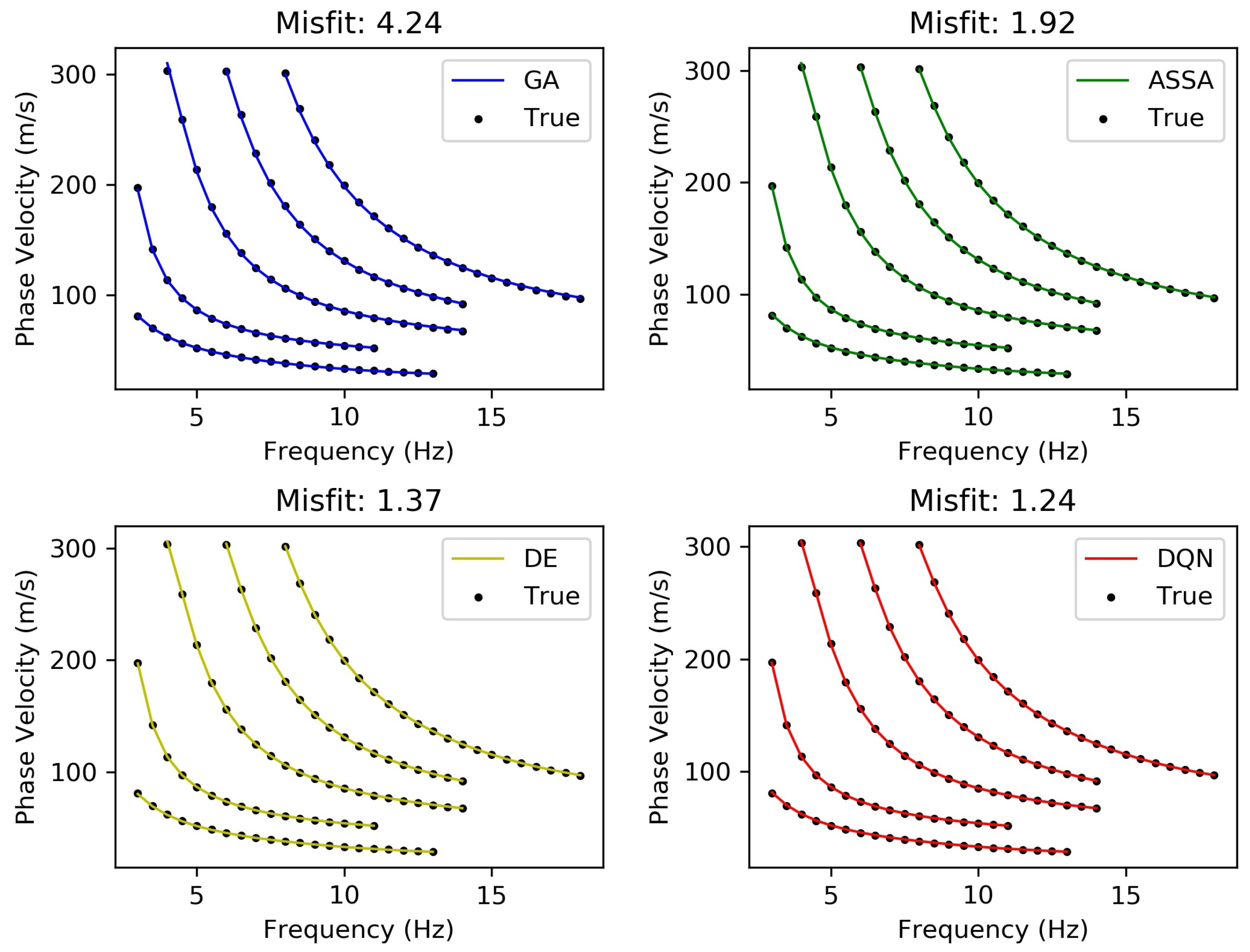
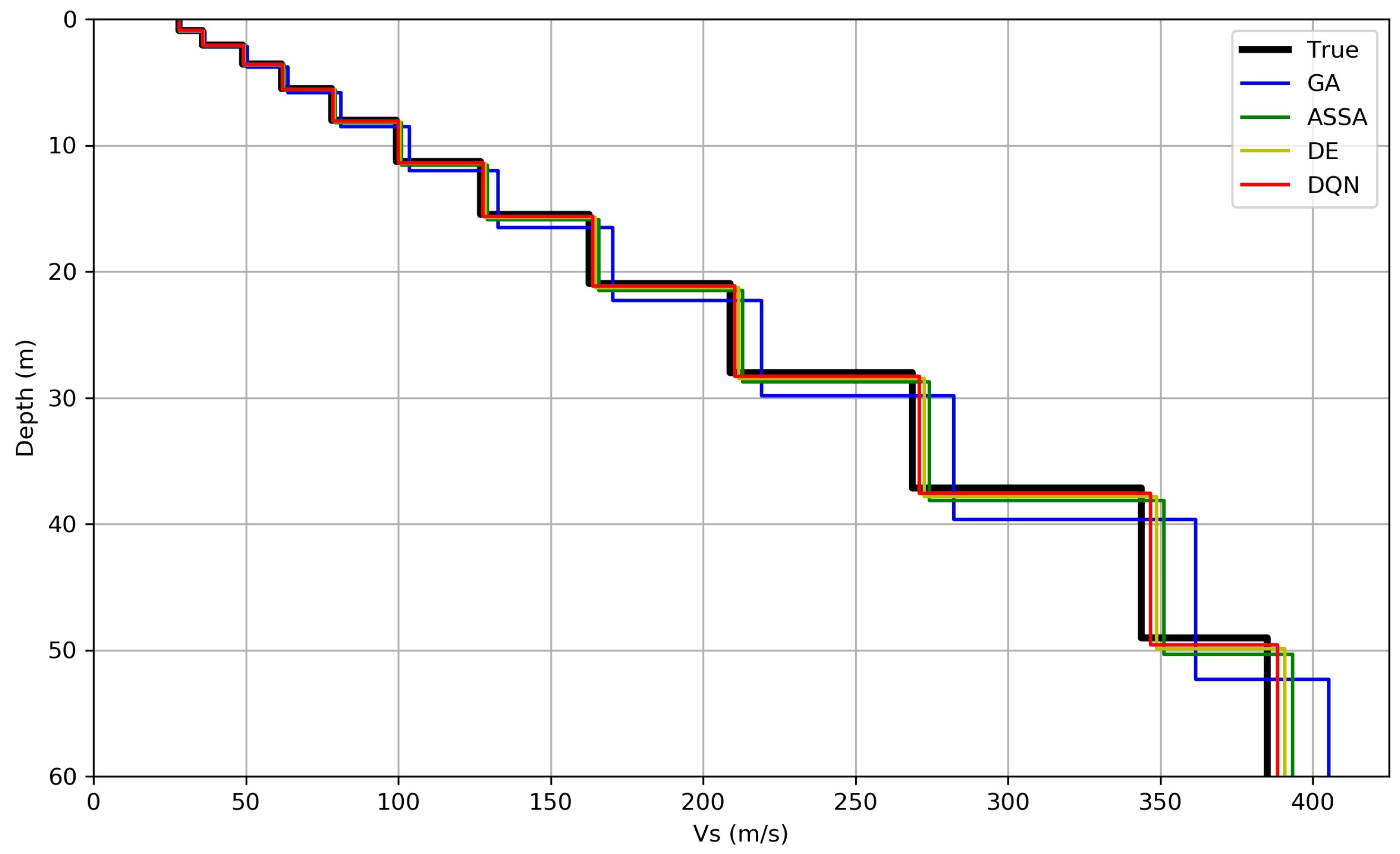
The estimated dispersion curves and shear wave velocity profiles are shown in Figure 7 and Figure 8, respectively. Their legends are the same as in Figure 3 and Figure 4, respectively.
The performance analysis for Case 2 is shown in Table 8, in which the bold fonts refer to the lowest relative error, misfit value, or running time over each row.
- The low-to-high ranking for the misfit values is the DQN framework, DE, ASSA, and GA. The ranking is consistent with the low-to-high ranking for the overall relative error. This trend is already found in Table 6.
- The DQN framework attains the lowest misfit, the shortest running time, and the lowest overall relative error compared to other candidate methods.
5.4. Discussion
Since the ground truth information is not available in many real scenarios, Table 9 expresses the performance comparison based on the metrics of misfit and running times and concludes the analysis in Section 5.2 and Section 5.3.
Table 9 demonstrates that the proposed framework performs a faster and lower misfit inversion (highlighted with bold fonts) compared to other methods. Furthermore, Figure 5 and Figure 6 illustrate that the proposed framework provides the inversion results with relatively lower uncertainties than other methods.
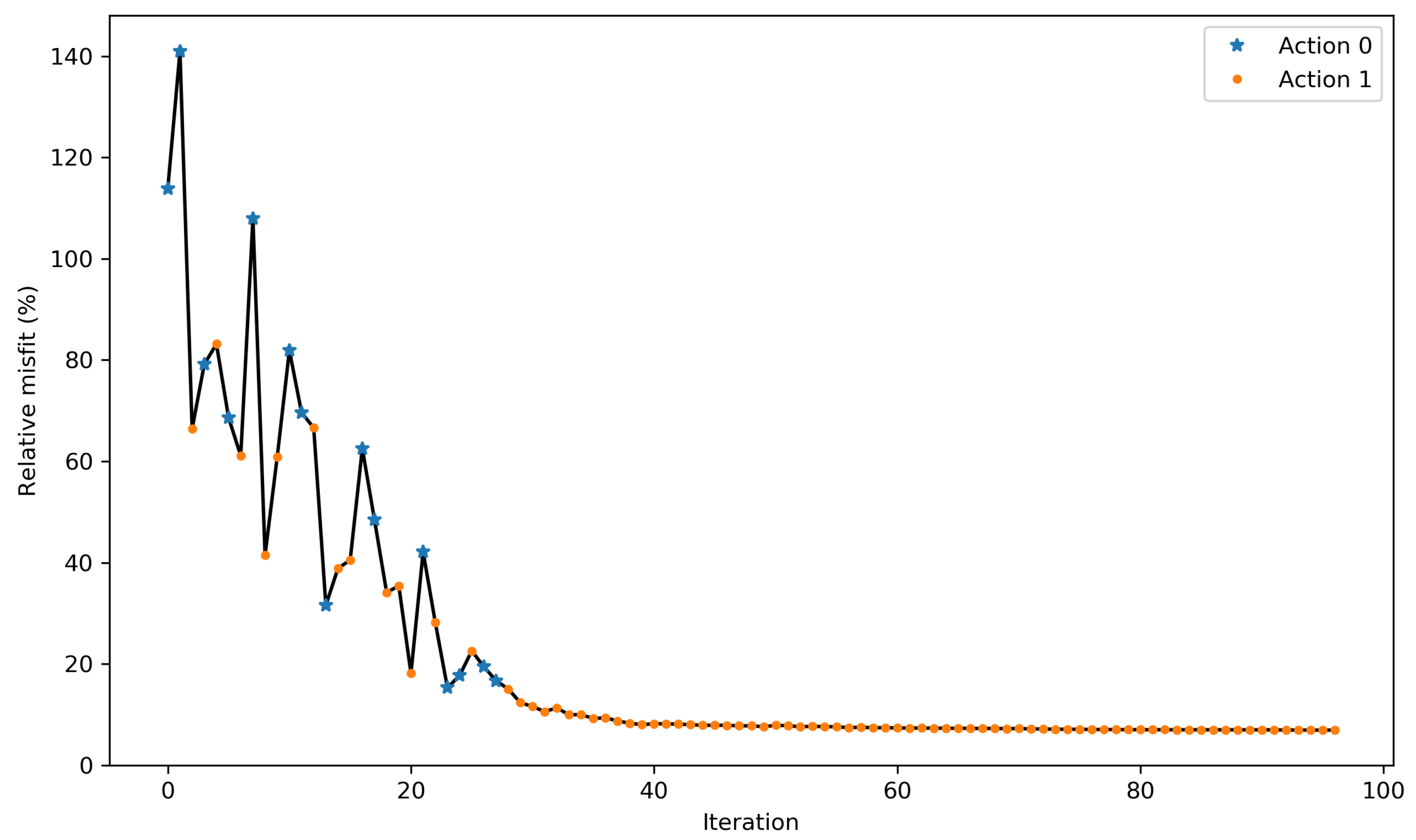
As mentioned in Section 4.2, Action 0 explores the parameter space more roughly since it compresses the search bounds in a relatively fast way. On the other hand, Action 1 is more suitable for finely exploring one local area in the parameter space. To understand the learned search strategy of the DQN framework, Figure 9 exhibits how the actions are executed by the DQN framework in an independent inversion for Case 1, where the blue star, the orange dot, and the black curve refer to Action 0, Action 1, and the relative misfit as a function of iteration numbers, respectively.
As shown in Figure 9, the agent executes Action 0 at the early stage of iterations and mainly executes Action 1 after that. This pattern can be interpreted as the DQN framework executing Action 0 at the early iterations to locate the rough area of the solution in the parameter space and executing a finer exploration (i.e., Action 1) after that to determine the final solution.
Note that we do not need to set a hard threshold for the agent to change the action from Action 0 to Action 1 because each independent inversion is initialized randomly. Furthermore, the relative misfit can exceed 100% at the first several iterations since the normalization factor is defined by a random initialization.
6. Conclusions
In this paper, a DQN-based framework for geoacoustic inversion is proposed. The framework can be defined as an optimization-based inversion method with a learnable search strategy, which keeps both advantages of optimization-based and ML-based approaches. Its performance is assessed by two numerical cases for estimating the shear wave velocity profile based on Scholte wave dispersion curves and compared with that of three popular optimization methods. Compared to the fastest conventional method, the running time of the proposed framework can be further reduced by 37.7% (Case 1) and 68.9% (Case 2), respectively. Compared to the best conventional method, the misfit of the proposed framework can be further reduced by 51.6% (Case 1) and 9.4% (Case 2), respectively. The results demonstrate the potential of DRL for geoacoustic inversion and the superior performance of the proposed framework. More specifically, the proposed framework can provide a faster, lower misfit, lower relative error, and lower uncertainty inversion. Please note that the application scope of the proposed framework is the whole geoacoustic inversion field. The proposed framework can easily be applied to different inversion tasks by using an appropriate forward model.
The future research direction will focus on the representation of the misfit space (i.e., the environment state) and the design of new available actions in the action space for the agent to explore the parameter space.
Implementation code availability: The code will be made available for the peer reviewers and the public upon request after the manuscript is published.
Author Contributions
Formal analysis, X.Z. and H.D.; funding acquisition, H.D.; methodology, X.Z. and H.D.; resources, X.Z. and H.D.; software, X.Z. and H.D.; writing—original draft, X.Z.; writing—review and editing, H.D. All authors have read and agreed to the published version of the manuscript.
Funding
This research received no external funding.
Institutional Review Board Statement
Not applicable.
Informed Consent Statement
Not applicable.
Data Availability Statement
The simulated dispersion curves will be made available upon request after the manuscript is published.
Acknowledgments
The authors would like to acknowledge the Norwegian Research Council and the industry partners of the GAMES consortium at NTNU for financial support (grant no. 294404). This work was partially supported by the SFI Centre for Geophysical Forecasting under grant 309960. Xiaoyu Zhu would like to acknowledge the China Scholarship Council (CSC) for the fellowship support (no. 201903170205).
Conflicts of Interest
The authors declare no conflict of interest.
Abbreviations
The following abbreviations are used in this manuscript:
| ML | machine learning |
| GA | genetic algorithm |
| DE | differential evolution |
| ASSA | adaptive simplex simulated annealing |
| DRL | deep reinforcement learning |
| DQN | deep-Q network |
| DQN framework | DQN-based framework for geoacoustic inversion |
| RMSE | root mean squared error |
| RE | relative error |
| LC | linear velocity gradient over a continuous half-space |
References
- Dong, H.; Dosso, S.E. Bayesian inversion of interface-wave dispersion for seabed shear-wave speed profiles. IEEE J. Ocean. Eng. 2011, 36, 1–11. [Google Scholar] [CrossRef]
- Dong, H.; Nguyen, T.D.; Duffaut, K. Estimation of seabed shear-wave velocity profiles using shear-wave source data. J. Acoust. Soc. Am. 2013, 134, 176–184. [Google Scholar] [CrossRef] [PubMed]
- Chapman, N.R.; Shang, E.C. Review of Geoacoustic Inversion in Underwater Acoustics. J. Theor. Comput. Acoust. 2021, 29, 2130004. [Google Scholar] [CrossRef]
- Yamanaka, H. Comparison of performance of heuristic search methods for phase velocity inversion in shallow surface wave method. J. Environ. Eng. Geophys. 2005, 10, 163–173. [Google Scholar] [CrossRef]
- Skyberg, N.S. Study of Optimization Algorithms for Underwater Acoustic Applications. Master’s Thesis, Institutt for Elektronikk og Telekommunikasjon, Norges teknisk-naturvitenskapelige universitet, Trondheim, Norway, 2013. [Google Scholar]
- Ohta, K.; Matsumoto, S.; Okabe, K.; Asano, K.; Kanamori, Y. Estimation of shear wave speed in ocean-bottom sediment using electromagnetic induction source. IEEE J. Ocean. Eng. 2008, 33, 233–239. [Google Scholar] [CrossRef]
- Snellen, M.; Simons, D.G.; Van Moll, C. Application of differential evolution as an optimisation method for geo-acoustic inversion. In Proceedings of the 7th European Conference on Underwater Acoustics, Delft, The Netherlands, 5–8 July 2004; pp. 721–726. [Google Scholar]
- Dosso, S.E.; Wilmut, M.J.; Lapinski, A.L. An adaptive-hybrid algorithm for geoacoustic inversion. IEEE J. Ocean. Eng. 2001, 26, 324–336. [Google Scholar] [CrossRef]
- Bianco, M.J.; Gerstoft, P.; Traer, J.; Ozanich, E.; Roch, M.A.; Gannot, S.; Deledalle, C.A. Machine learning in acoustics: Theory and applications. J. Acoust. Soc. Am. 2019, 146, 3590–3628. [Google Scholar] [CrossRef] [PubMed]
- Piccolo, J.; Haramuniz, G.; Michalopoulou, Z.H. Geoacoustic inversion with generalized additive models. J. Acoust. Soc. Am. 2019, 145, EL463–EL468. [Google Scholar] [CrossRef]
- Shen, Y.; Pan, X.; Zheng, Z.; Gerstoft, P. Matched-field geoacoustic inversion based on radial basis function neural network. J. Acoust. Soc. Am. 2020, 148, 3279–3290. [Google Scholar] [CrossRef]
- Van Komen, D.F.; Neilsen, T.B.; Howarth, K.; Knobles, D.P.; Dahl, P.H. Seabed and range estimation of impulsive time series using a convolutional neural network. J. Acoust. Soc. Am. 2020, 147, EL403–EL408. [Google Scholar] [CrossRef]
- Mnih, V.; Kavukcuoglu, K.; Silver, D.; Graves, A.; Antonoglou, I.; Wierstra, D.; Riedmiller, M. Playing atari with deep reinforcement learning. arXiv 2013, arXiv:1312.5602. [Google Scholar]
- Gu, S.; Holly, E.; Lillicrap, T.; Levine, S. Deep reinforcement learning for robotic manipulation with asynchronous off-policy updates. In Proceedings of the 2017 IEEE international conference on robotics and automation (ICRA), Singapore, 29 May–3 June 2017; pp. 3389–3396. [Google Scholar]
- Silver, D.; Schrittwieser, J.; Simonyan, K.; Antonoglou, I.; Huang, A.; Guez, A.; Hubert, T.; Baker, L.; Lai, M.; Bolton, A.; et al. Mastering the game of go without human knowledge. Nature 2017, 550, 354–359. [Google Scholar] [CrossRef] [PubMed]
- Joo, H.; Lim, Y. Traffic Signal Time Optimization Based on Deep Q-Network. Appl. Sci. 2021, 11, 9850. [Google Scholar] [CrossRef]
- Zhou, S.; Liu, J.; Hou, D.; Zhong, X.; Zhang, Y. Autonomous penetration testing based on improved deep q-network. Appl. Sci. 2021, 11, 8823. [Google Scholar] [CrossRef]
- Park, J.H.; Farkhodov, K.; Lee, S.H.; Kwon, K.R. Deep reinforcement learning-based DQN agent algorithm for visual object tracking in a virtual environmental simulation. Appl. Sci. 2022, 12, 3220. [Google Scholar] [CrossRef]
- Gao, S.J.; Li, Y.T.; Geng, T.W. Deep Reinforcement Learning-Based Relay Selection Algorithm in Free-Space Optical Cooperative Communications. Appl. Sci. 2022, 12, 4881. [Google Scholar] [CrossRef]
- Guan, Z.; Wang, Y.; He, M. Deep Reinforcement Learning-Based Spectrum Allocation Algorithm in Internet of Vehicles Discriminating Services. Appl. Sci. 2022, 12, 1764. [Google Scholar] [CrossRef]
- Zhao, S.; Wang, L.; Zhao, Z.; Bi, L. Study on the Autonomous Walking of an Underground Definite Route LHD Machine Based on Reinforcement Learning. Appl. Sci. 2022, 12, 5052. [Google Scholar] [CrossRef]
- Qin, Z.; Zhang, X.; Zhang, X.; Lu, B.; Liu, Z.; Guo, L. The UAV Trajectory Optimization for Data Collection from Time-Constrained IoT Devices: A Hierarchical Deep Q-Network Approach. Appl. Sci. 2022, 12, 2546. [Google Scholar] [CrossRef]
- Asaf, K.; Khan, B.; Kim, G.Y. Wireless Lan Performance Enhancement Using Double Deep Q-Networks. Appl. Sci. 2022, 12, 4145. [Google Scholar] [CrossRef]
- Wang, H.; Liu, Y.; Yin, C.; Li, J.; Su, Y.; Xiong, B. Stochastic inversion of magnetotelluric data using deep reinforcement learning. Geophysics 2022, 87, E49–E61. [Google Scholar] [CrossRef]
- Kolobov, A. Planning with Markov decision processes: An AI perspective. Synth. Lect. Artif. Intell. Mach. Learn. 2012, 6, 1–210. [Google Scholar]
- Wu, G.; Dong, H.; Ke, G.; Song, J. Shear-Wave Tomography Using Ocean Ambient Noise with Interference. Remote Sens. 2020, 12, 2969. [Google Scholar] [CrossRef]
- Saito, M. DISPER80: A subroutine package for the calculation of seismic normal-mode solutions. In Seismological Algorithms; Doornbos, D.J., Ed.; Academic Press: New York, NY, USA, 1988; pp. 293–319. [Google Scholar]
- Thomson, W.T. Transmission of elastic waves through a stratified solid medium. J. Appl. Phys. 1950, 21, 89–93. [Google Scholar] [CrossRef]
- Haskell, N.A. The dispersion of surface waves on multilayered media. Bull. Seismol. Soc. Am. 1953, 43, 17–34. [Google Scholar] [CrossRef]
- Paszke, A.; Gross, S.; Massa, F.; Lerer, A.; Bradbury, J.; Chanan, G.; Killeen, T.; Lin, Z.; Gimelshein, N.; Antiga, L.; et al. Pytorch: An imperative style, high-performance deep learning library. In Proceedings of the Advances in Neural Information Processing Systems 32 (NeurIPS 2019), Vancouver, BC, Canada, 8–14 December 2019. [Google Scholar]
Figure 1.
The general workflow of geoacoustic inversion.

Figure 2.
DQN-based search strategy.

Figure 3.
The estimated dispersion curves with the ground truth in Case 1.

Figure 4.
The estimated shear wave velocity profiles with the ground truth in Case 1.

Figure 5.
Statistic analysis of over the candidate methods.

Figure 6.
Statistic analysis of over the candidate methods.

Figure 7.
The estimated dispersion curves with the ground truth in Case 2.

Figure 8.
The estimated shear wave velocity profiles with the ground truth in Case 2.

Figure 9.
Action execution by the DQN framework in an independent inversion.


Table 1.
Architecture of the neural network in the DQN framework.
| Name | Input Channel | Output Channel |
|---|---|---|
| Dense layer 1 | 6 | 1024 |
| ReLU | - | - |
| Dense layer 2 | 1024 | 1024 |
| ReLU | - | - |
| Dense layer 3 | 1024 | 2 |
Table 2.
Hyperparameters of the DQN framework.
| Item | Value |
|---|---|
| Mini-batch size | 32 |
| Memory size | 100,000 |
| Update frequency | 4 |
| Discount factor | 0.9 |
| Learning rate | 0.0001 |
| Factor in greedy strategy | 0.9 |
| Training epoch | 300 |
Table 3.
Preset parameters of the candidate methods.
| Algorithm | Description | Value |
|---|---|---|
| All | Maximum of iteration () | 100 |
| Number of sampling per iteration (k) | 200 | |
| Threshold of misfit () | 10 (m/s) | |
| Threshold of convergence () | 0.1 | |
| GA and DE | Mutation rate | 0.001 |
| Population size | 200 | |
| ASSA | Temperature reduction factor | 0.995 |
Table 4.
Geoacoustic model for Case 1.
| Layer | h (m) | () | (m/s) | (m/s) |
|---|---|---|---|---|
| 0 (Ocean) | 125 | 1.0 | 1490 | 0 |
| 1 | 35 | 1.5 | 1750 | 365 |
| 2 | 89 | 1.8 | 2000 | 696 |
| 3 | 125 | 2.0 | 3500 | 878 |
| 4 | 224 | 2.2 | 3750 | 1060 |
| 5 (Half-space) | 956 | 2.1 | 3250 | 1140 |
Table 5.
Search bounds for Case 1.
| Layer | h (m) | (m/s) |
|---|---|---|
| 0 (Ocean) | - | - |
| 1 | [10, 70] | [100, 500] |
| 2 | [40, 120] | [250, 850] |
| 3 | [50, 350] | [500, 1200] |
| 4 | [50, 650] | [800, 1500] |
| 5 (Half-space) | - | [700, 1800] |
Table 6.
Performance analysis for Case 1.
| GA | ASSA | DE | DQN Framework | |
|---|---|---|---|---|
| 3.27% | 2.21% | 2.17% | 0.39% | |
| 7.26% | 0.56% | 3.28% | 2.05% | |
| 10.31% | 0.68% | 2.72% | 0.16% | |
| 11.38% | 14.30% | 20.36% | 4.83% | |
| 2.03% | 1.03% | 1.21% | 0.61% | |
| 0.26% | 0.14% | 0.08% | 0.87% | |
| 1.98% | 0.31% | 0.52% | 0.04% | |
| 1.00% | 0.40% | 0.59% | 0.06% | |
| 1.06% | 1.84% | 2.49% | 0.61% | |
| Misfit (m/s) | 17.60 | 12.46 | 15.72 | 6.03 |
| Running time (s) | 181.03 | 876.29 | 371.01 | 112.70 |
Table 7.
LC model for Case 2.
| Layer | h (m) | () | (m/s) | (m/s) | (m/s) |
|---|---|---|---|---|---|
| Ocean | 364 | 1.0 | 1490 | 0 | 0 |
| Sediment | 49 | 1.8 | 1700 | 28 | 385 |
| Half-space | 200 | 1.8 | 2000 | 385 | 385 |
Table 8.
Performance analysis for Case 2.
| GA | ASSA | DE | DQN Framework | |
|---|---|---|---|---|
| H | 6.74% | 2.74% | 1.85% | 1.22% |
| 1.48% | 0.58% | 0.40% | 0.32% | |
| 5.24% | 2.18% | 1.50% | 0.89% | |
| Misfit (m/s) | 4.24 | 1.92 | 1.37 | 1.24 |
| Running time (s) | 176.92 | 340.60 | 468.13 | 53.78 |
Table 9.
Overall performance analysis.
| GA | ASSA | DE | DQN Framework | |||||
|---|---|---|---|---|---|---|---|---|
| Case 1 | Case 2 | Case 1 | Case 2 | Case 1 | Case 2 | Case 1 | Case 2 | |
| Misfit (m/s) | 17.60 | 4.24 | 12.46 | 1.92 | 15.72 | 1.37 | 6.03 | 1.24 |
| Running time (s) | 181.03 | 176.92 | 876.29 | 340.60 | 371.01 | 468.13 | 112.70 | 53.78 |
Publisher’s Note: MDPI stays neutral with regard to jurisdictional claims in published maps and institutional affiliations. |
© 2022 by the authors. Licensee MDPI, Basel, Switzerland. This article is an open access article distributed under the terms and conditions of the Creative Commons Attribution (CC BY) license (https://creativecommons.org/licenses/by/4.0/).
Share and Cite
MDPI and ACS Style
Zhu, X.; Dong, H. Shear Wave Velocity Estimation Based on Deep-Q Network. Appl. Sci. 2022, 12, 8919. https://0-doi-org.brum.beds.ac.uk/10.3390/app12178919
AMA Style
Zhu X, Dong H. Shear Wave Velocity Estimation Based on Deep-Q Network. Applied Sciences. 2022; 12(17):8919. https://0-doi-org.brum.beds.ac.uk/10.3390/app12178919
Chicago/Turabian StyleZhu, Xiaoyu, and Hefeng Dong. 2022. "Shear Wave Velocity Estimation Based on Deep-Q Network" Applied Sciences 12, no. 17: 8919. https://0-doi-org.brum.beds.ac.uk/10.3390/app12178919
Note that from the first issue of 2016, this journal uses article numbers instead of page numbers. See further details here.