Article

Towards the Integration and Automation of the Design Process for Domestic Drinking-Water and Sewerage Systems with BIM

by
Edison Atencio
1,2,*,
Pablo Araya
1,
Francisco Oyarce
1,
Rodrigo F. Herrera
1,
Felipe Muñoz-La Rivera
1,3,4 and
Fidel Lozano-Galant
2
1
School of Civil Engineering, Pontificia Universidad Católica de Valparaíso, Av. Brasil 2147, Valparaíso 2340000, Chile
2
Department of Civil Engineering, Universidad de Castilla-La Mancha, Av. Camilo Jose Cela s/n, 13071 Ciudad Real, Spain
3
School of Civil Engineering, Universitat Politecnica de Catalunya, 08034 Barcelona, Spain
4
International Center for Numerical Methods in Engineering (CIMNE), 08034 Barcelona, Spain
*
Author to whom correspondence should be addressed.
Submission received: 30 June 2022 / Revised: 2 September 2022 / Accepted: 6 September 2022 / Published: 9 September 2022

Abstract

:
The use of building information modelling (BIM) in construction projects is expanding, and its usability throughout building lifecycles, from planning and construction to operation and maintenance, is gaining increasing proof. In the design of domestic drinking-water and sewerage systems (DDWSSs), BIM focuses on coordinating disciplines and their design. Despite studies promoting BIM environments for DDWSSs that take into account the regulatory frameworks of corresponding countries, these efforts do not include the use of parametric tools that enhance the efficiency of the design process. Therefore, engineers still use conventional 2D design, which requires many rounds of iteration, and manual work is also generally still used. In this research, we developed and validated an intuitive methodology for solving a specific DDWSS problem, using a design science research method (DSRM) as an applied science approach. This was addressed by developing an artefact and validating it through two case studies. The obtained solution combines BIM models and parametric tools to automate the manual activities of the traditional design method. This article aims to bring abstract BIM concepts into practice and encourage researchers and engineers to adopt BIM for DDWSSs.

1. Introduction

Mechanical, electrical and plumbing (MEP) design and coordination tools have an important role in the design process [1]. However, the use of building information modelling (BIM) in MEP disciplines has traditionally focused on coordinating specialities and not on the actual design of each of the specialities [2]. The design and capacity of pipe network systems—as well as domestic drinking-water and sewerage systems (DDWSSs)—and their critical points/connections inside a building may affect the building components, such as architectural spaces and structural systems. Service systems, such as heating, ventilation and air conditioning (HVAC), can also be affected [1].
Previous studies promoted the design of drinking water facilities in BIM environments in order to take into account the regulatory frameworks of corresponding countries [3].
However, these efforts did not include the use of parametric tools that increase the efficiency of the design process. The MEP tool from one of the most common BIM software packages [4], REVIT, is based on the International Plumbing Code (IPC), but it cannot be edited and it does not take into account different country regulations, preventing its use as a drinking water design tool
The use of BIM for plumbing systems has also been explored in the context of asset management in the building operation stages, even using 4.0 technologies; e.g., augmented reality and sensors [5]. However, these uses are mainly focused on visualisation-based analysis and not the design of plumbing systems.
This research developed and validated an intuitive methodology for solving a specific problem in DDWSS design, using a design science research method (DSRM) as an applied science approach. This problem is addressed by developing a methodology as a workflow. To validate the proposed methodology in the case of the Chilean standard for DDWSS design, two case studies (one simple and one complex) were developed and compared with the traditional DDWSS design methodology. These case studies were validated in terms of the effort required, the complexity, the real automation level and the quality of the results. The obtained solution combines BIM models and parametric tools to automate the manual activities from the traditional design method.
This work aims to bring abstract BIM concepts into practice and encourage researchers and MEP engineers to adopt BIM for DDWSSs and to automate manual tasks. This issue is relevant in light of the findings of the most recent, extensive BIM report developed in Chile [6], which reveals that the MEP speciality is the least advanced in BIM in terms of adherence to BIM standards, motivation, satisfaction and perceived value.
The remainder of this paper is organised as follows. In Section 2, the research methodology is described. Section 3 discusses the background of this paper through a literature review. Section 4 describes the proposed workflow for DDWSS design. The case studies are developed in Section 5, and their results are provided and discussed in Section 6. Finally, the conclusions of this paper are described in Section 7.

2. Research Methodology

This research is based on a design science research method (DSRM) suitable for engineering innovation research projects [7]. The DSRM is structured in five stages: (1) identification of observed problems and motivations, (2) definition of the potential solution, (3) design and development, (4) demonstration and (5) evaluation. Figure 1 shows a summary of these stages, along with their objectives and the tasks and tools required.
The first stage focused on understanding the challenges in DDWSS design project approaches. Moreover, the current research and designing standards were collected; these include the Regulation on Domestic Installations of Drinking Water and Sewerage (Reglamento de Instalaciones Domiciliarias de Alcantarillado y Agua Potable, RIDAA [8]), a Chilean standard. Additionally, complementary standards are applied for verification, determination of materials, identification of the ranges of allowable values and the presentation of deliverables. For this paper, the following Chilean standards (https://www.inn.cl/nch-aprobadas, Accessed on 8 September 2022) were used: NCh 398, NCh 399, NCh 951, NCh 1635, NCh 2038, NCh 2485, NCh 2592 and NCh 2836.
The literature review was used a tool in this first stage to identify research articles and documented projects related to key concepts: automation using BIM, parametric design automation and plumbing design in BIM environments. The Google Scholar, Scopus and Web of Science platforms were used to search for relevant literature published between 2000 and 2022.
In the second stage, we developed automatised methods for optimising time, costs, human resources and the overall development of DDWSS design projects. This goal was achieved by creating algorithms and automatic processes. The parameterisation of regulatory calculation guidelines in a BIM environment reduces the amount of manual work required during the design stage of DDWSS projects.
In the third stage, we identified a sequence of activities based on the literature review and determined the different functionalities of the selected software for the development of the expected solution:
  • Defining the format for the input data of the project so that it corresponds to parameters obtained both directly and indirectly from the three-dimensional model;
  • Defining the way to extract these data into spreadsheets, if required;
  • Defining the procedure for transferring the complementary project information that corresponds to the indirect input data of the model—i.e., project characteristics that cannot be obtained from the model and must be entered by the user;
  • Determining the iterative method for the calculation and verification of the resulting parameters as a convergence process;
  • Defining the method for the insertion of data into the BIM software, which are then returned to the model and modify the initial values of the project—for instance, pipe diameters;
  • Configuring deliverables corresponding to floor plans and tabulations with results in a standard plan, as defined by the RIDAA.
In the fourth stage, the described workflow was implemented for a simple case study with basic characteristics involving a residential building with a distributed system on a single floor. This process involved checking the functionality of the algorithm and the data management for the design parameters.
Finally, in the fifth stage, a more complex case study was introduced to evaluate the behaviour of the programmed algorithms. This case study corresponded to a known and previously solved real-world project, which allowed the results obtained to be compared with values resulting from traditional calculation. The comparison of the results was conducted by calculating the relative errors with the known values of the project.

3. Background

This section is organised into as follows: firstly, digitalisation processes in the building sector are reviewed. Interoperability problems among disciplines are also analysed. Then, the traditional design method meeting the requirements of DDWSSs is analysed. Finally, the application of BIM for the design of DDWSSs is presented.

3.1. Digitalisation of the Construction Sector

MEP systems provide particular, basic services that help to expand and complement the economic efficiency, utility and durability of buildings and create comfortable environments throughout the entire lifecycles of buildings [9]. These services commonly include heating, ventilation and air conditioning (HVAC), along with electric, electronic, plumbing and anti-power systems [10]. For housing projects, the functionality and efficiency of these facilities can have a huge impact on a project’s sustainability and success [11]. As building designs and requirements evolve into more complete and complex installations [12], progress in computational technologies and their continuous integration into the construction industry have proven effective in dealing with these new challenges [13].
BIM represents a work methodology that combines information and communication technologies, improving project management and facilitating the application of international standards throughout buildings’ lifecycles [12]. BIM encompasses digital modelling, simulation, coordination, optimisation and automatic drawing generated by computers; it facilitates information storage and exchange between different users, enhancing project understanding and outcome development [14]. A major challenge of the BIM methodology is the accurate exchange of information between the software of different disciplines (interoperability) [15]. In addition, working with BIM requires collaborative work methodologies that focus on information exchange, coordination and collaboration among the stakeholders [16].
Solving problems of interoperability between the software for different disciplines is one of the major challenges in implementing the BIM methodology. In fact, this kind of problem can also appear within the software of a single company. Table 1 provides a selection of the many studies in the literature dealing with the interoperability problems in Autodesk® software. This table includes the aim of the study, the different software used for the modelling (modelling software) and the software used to deliver the information (visual programming tool). These visual programming language software packages are based on textual programming languages; they visually represent actions composed of linear string sequences of code. The analysis in Table 1 shows that interoperability problems can be found in different disciplines (such as facility management, heritage, coordination and MEP). Regarding the software analysis, the table shows that Revit is the most common modelling software, and, for the delivery of the information, visual programming language software packages (Dynamo or Grasshopper) are commonly used.

3.2. Traditional Design Method for DDWSSs

The spatial and mechanical design of sanitary plumbing and drainage systems and components has not undergone substantial change in recent years [25]. CAD and 2D layouts are still suggested by standard regulations for the calculation methodology and required as the official presentation format [26]. At present, calculation methods must be guided by the specific codes and standards of the relevant country. The design, installation and specifications of plumbing systems in buildings are covered by guidelines [27]. Although standards specify equations, limits, considerations and minimum criteria, different hydraulic formulations have their respective justifications. In this context, RIDAA is currently the official code/regulation in Chilean practice.
The conventional method for DDWSS design involves laborious work based on permanent user interaction with different professional software packages [6,28]. Data manipulation and association comprise a highly manual process. These methods generally involve the following steps:
  • The design process starts with interpreting two-dimensional models (2D/CAD) and visualising and locating relevant data according to the potential input parameters presented in the project floor plan, such as types of plumbing fixtures, locations, quantities, rooms, equipment and other operational function requirements;
  • Specialist sub-contractors use this information to develop their system routing, connecting elements of all building systems in compliance with architectural and structural designs [29]. Then, spreadsheets are commonly used to discretise data about piping systems, adding conditions and general project specifications that are not incorporated in the data extracted from the layout [6,28];
  • These spreadsheets, as shown in RIDAA’s content, represent the official calculation and presentation formats. The system, material and geometric parameters of pipe paths are adjusted until an optimal solution is reached: the process is repeated until design parameters reach acceptable values according to the code ranges for pressure/flow rates and slopes in drinking water networks and drainage networks, respectively [26];
  • Finally, contractors summarise and compile results, incorporating them into a two-dimensional model of the floor plans, elevations and isometrics, according to the symbology defined by the standards. This symbology is established for the water supply and sanitary treatment companies in the area, which are responsible for providing and maintaining connections with the public network.
Urbanisation through residential projects involves integration of several engineering specialisms. Contractors develop their models individually, following project requirements for optimal functionality. Therefore, they generally do not consider other systems from an interrelated viewpoint [29]. Coordination is needed to detect and eliminate spatial and functional interferences among systems; drawings for multiple layouts must be overlaid and compared [30]. In two-dimensional design, visualisation is limited, the data-sharing process easily comes into conflict with the work of other professionals and work lacks efficiency [31]. This repeatedly generates rework and coordination meetings, as re-routing systems and the relocation of elements are required to avoid clashes with a significantly increasing number of iterations [29]. Moreover, these issues are time-consuming and expensive [12]. When such changes occur later in the construction stage, unscheduled delays, and even accidents, can occur. These situations force engineers to respond to and resolve these situations quickly and may cause confusion and problems for technicians and/or malfunctions in installations [32].

3.3. BIM as a DDWSS Design Tool

BIM modelling utilises a virtual platform to design and develop building projects. The Autodesk® Revit® platform integrates operational and functional characteristics, providing strong tools for the management of relevant and necessary information when the BIM methodology is used. MEP design tools have been developed and represent a small part of Autodesk’s priority of developing BIM solutions. At this stage, these efforts are intended to provide all the tools needed by MEP engineers, and Autodesk® is focused on evolving into a single-source BIM solution for the AEC community.
In DDWSS design projects, BIM modelling tools generate a database with element, component and technical information in the form of either geometric (diameter, elevation, length, slope) or mechanical parameters (materials, roughness, flow rate, flow velocity, pressure). These elements can be modified as a project requires, allowing parameters to be modified in conformity with geometrical or model connections, which makes the modelling process more efficient and intuitive [33]. However, these tools lack the potential for customisation, and adaptation to local design guidelines can still be achieved through traditional approaches [27,34].
Parametric modelling combines 3D modelling with external data, enhancing information storage within various project elements as designers generate the 3D model, set instance parameters and place the model in the 3D interface. This information can be used for different projects after saving the initial configurations for further usage [35,36]. Among the parametric programming tools, Dynamo can be highlighted. This tool allows 3D elements to be correlated and enables spatial control with geometric and parametric information. The above allows custom data management and visualisation; all changes appear as analytical data in real time [37,38].

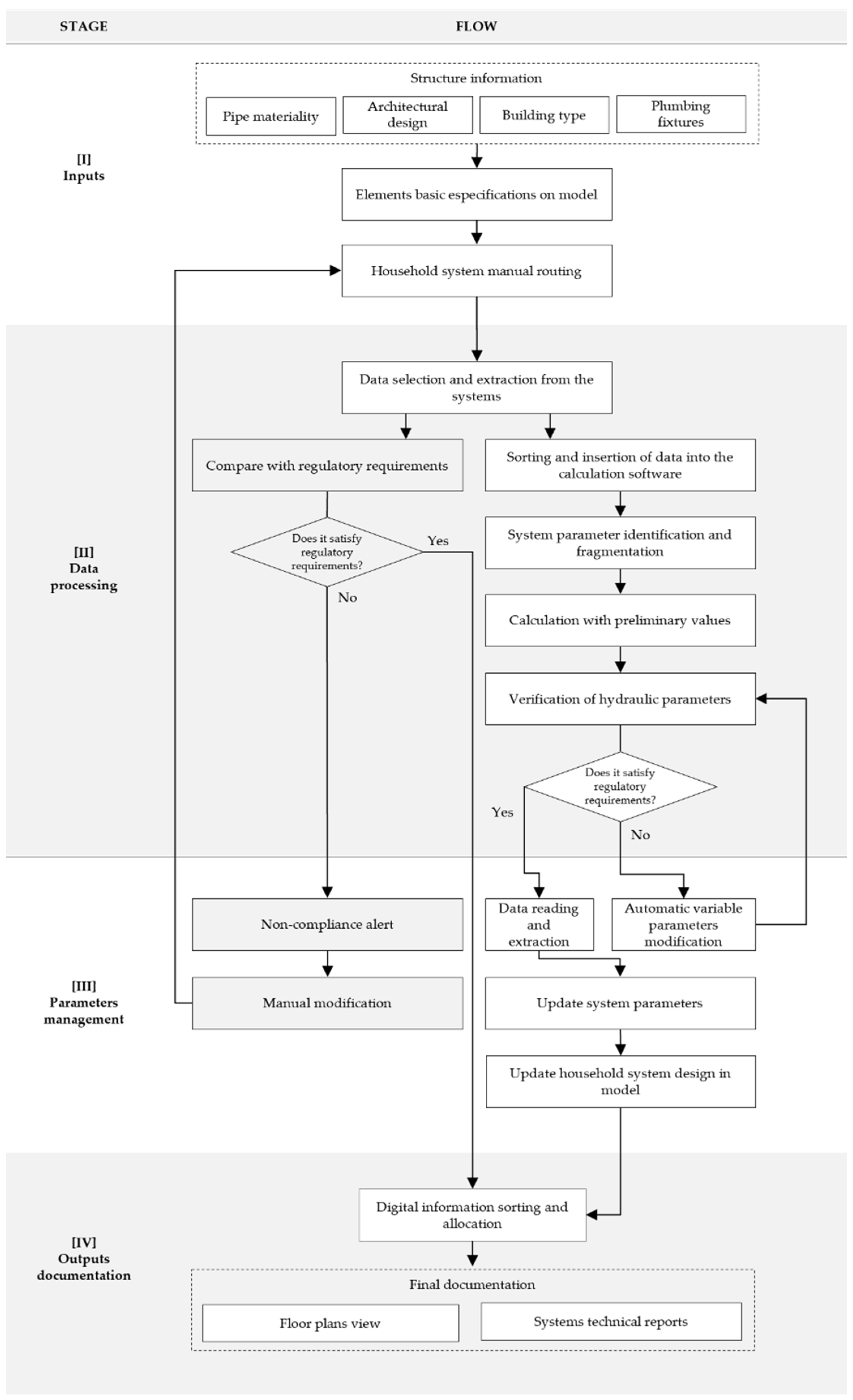
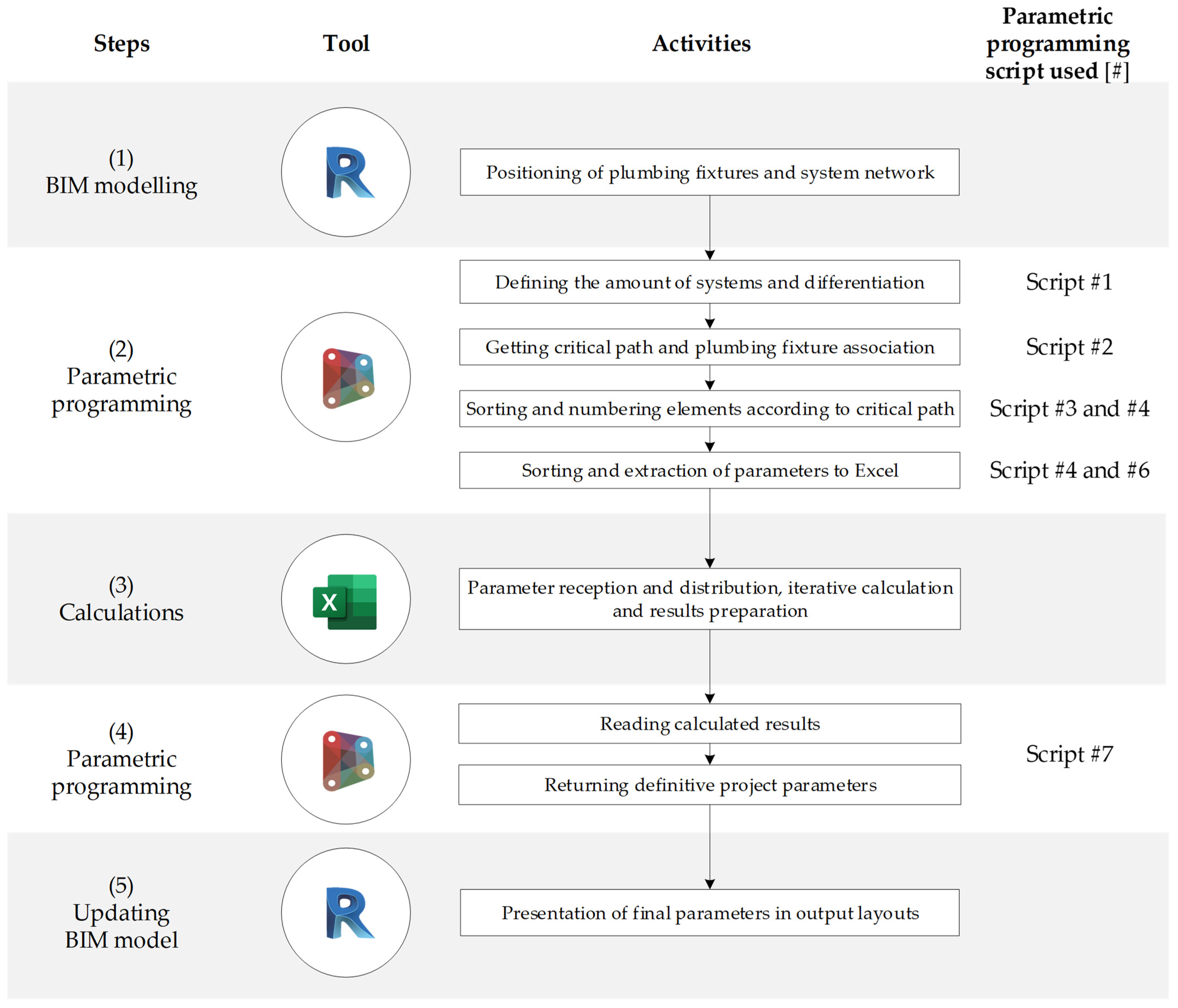
4. Proposed Workflow for DDWSS Design

When proposing a sequence of semi-automated activities for DDWSS design, design standards, technical recommendations, software characteristics, the scope of use, work templates, interoperability between software packages and interface usability must be considered in terms of the effort required. Nevertheless, not all the tasks in a process may be suitable for automation. Complexity levels and the manual work required to perform a task impact the level of effort required. Therefore, as a rule, if automating a task involves more work than performing it manually, it can be considered to either not be automatable or to be a high-cost automation task [39].
The workflow and algorithms developed in this research allow the automation of the development of MEP design in building projects. The workflow provides simple steps for the automation of the design process. Furthermore, the algorithms developed in Dynamo allow the recognition of a BIM project in the Revit environment, identifying its elements and constraints, enabling its calculation with different standards in Excel and updating the design information for the BIM environment.
Figure 2 shows the proposed workflow, including the automation and documentation processes. It consists of four stages: (I) inputs, (II) data processing, (III) parameter management and (IV) output documentation.
Figure 2 shows the steps for automating the design process for DDWSSs. The formulations and calculation guidelines are based on the RIDAA. These stages are easily distinguishable in order to intuitively guide users through the automation process in a simple way. This workflow represents only a guide for the development; the details of the individual sections are given below. Later, in Section 5, the detailed workflows and associated codes for the automation process for both the design and verification of the required MEP elements are presented.

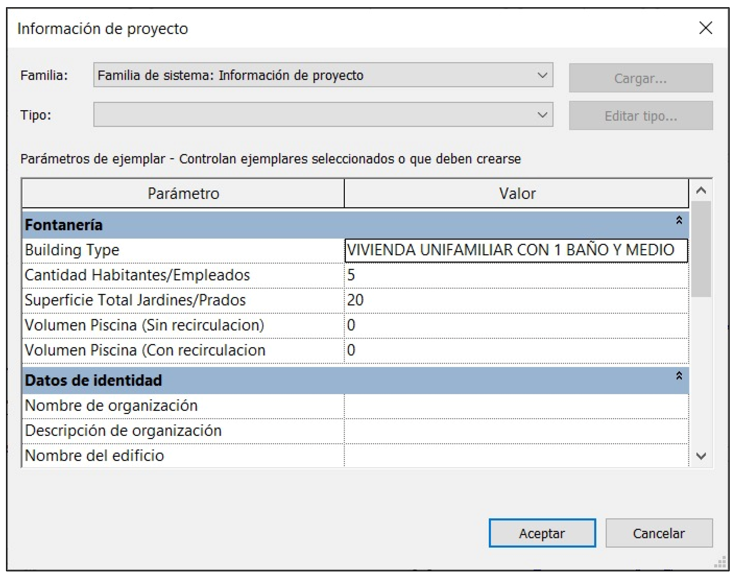
4.1. Inputs for Automation

For conceptual design, the preliminary information on the structure is delivered by an architectural design that provides the basic conditions for DDWSS operation, such as the type of building, the location, the number of occupants or users, the estimated consumption and the existing public distribution and collection networks [26]. It is then necessary to define the type, location and quantity of artefacts used in the building in order to connect them and create a system through a manual routing process. The purpose of the manual routing process is to facilitate the modeller’s freedom and establish criteria for the design of the network. Within the routing process, the materials and preliminary diameters of the pipes must be assigned, as well as any mechanical systems that may be required [40].
As a preliminary step for the generation of BIM project models, the different elements used for the calculations must be configured in Autodesk® Revit®, especially those belonging to MEP systems. These elements are included by default with predefined parametric values. Autodesk® Revit® contains a database of default families and family types, the configuration of which is predefined according to International Plumbing Code (IPC) specifications. It is necessary to modify and integrate objects’ families according to the regulations relating to their characteristics, dimensions and mechanical parameters applicable in the country where the automation process will be applied. This also applies to pipe families, for which—although they have a predefined database—it is necessary to add new family types. In the case of materials, it is necessary to add those that are available in the market and those that are increasingly used to establish the commercial diameters for the modelling.
Regarding the system’s artefacts, for each sanitary fixture, the corresponding acronym, installed flow rates, height and inlet and outlet diameters must be defined. Each pipe section drawn will be subject to both geometrical and mechanical constraints, so it is important to consider the performance of the connections of the elements in the model when building the piping system. It is thus necessary to undertake detailed modelling of each component of each system. All the fittings and connectors must be described and positioned consistently in order to avoid any deviations or differences in the data readings provided by the model. Moreover, the modeller must correctly select the type of system to which each traced pipe belongs; i.e., the cold-water, hot-water or drainage systems.
In sewerage systems, it is important to indicate the intended use of the sanitary fixtures according to the type of building and the number of people to be served in order to correctly define the wastewater flow that returns to the public system. Water flow sewage systems are gravity-fed; therefore, certain considerations must be taken into account when laying out the pipes so as not to generate points at which solid waste can be deposited and obstruct the continuous discharge of the flow. According to the regulations, a minimal pipe slope must be provided to allow for self-cleaning, the creation of geometries with closed singularities should be avoided and manholes should be placed correctly.

4.2. Data Processing and Parameter Management

In this part of the study, the parameters of the sanitary devices present in the model were identified and extracted, then ordered and tabulated in such a way that the pipe sections can be automatically generated. In the case of drinking water systems, the creation of tables for export is intended for the iterative calculation of their parameters, which are then returned to the model, replacing the existing values. In the case of sewerage systems, data extraction is carried out to verify the slope, waste load and diameter parameters, which are compared with those from the regulations used. If the regulatory values are not satisfied, an alert is shown indicating regulatory non-compliance; this means that the parameters in the model must be manually modified and, subsequently, re-verified until they comply with the permitted ranges.
In addition, depending on the regulations used when carrying out automation, it may be necessary to make practical changes, replacing the designer’s criteria when establishing ranges of values for certain parameters that may be subject to special external conditions or simply in order to maximise safety.

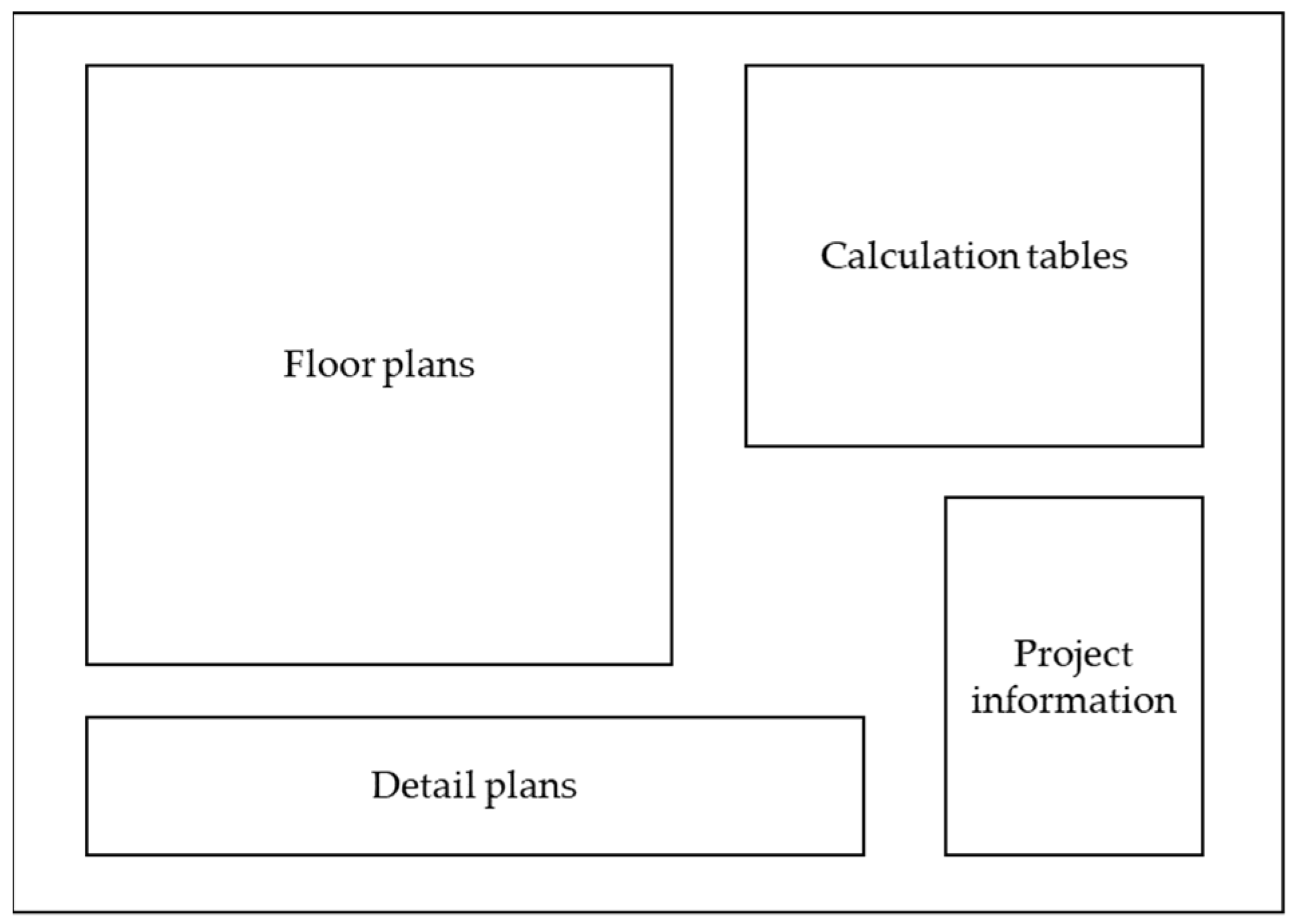
4.3. Output Documentation
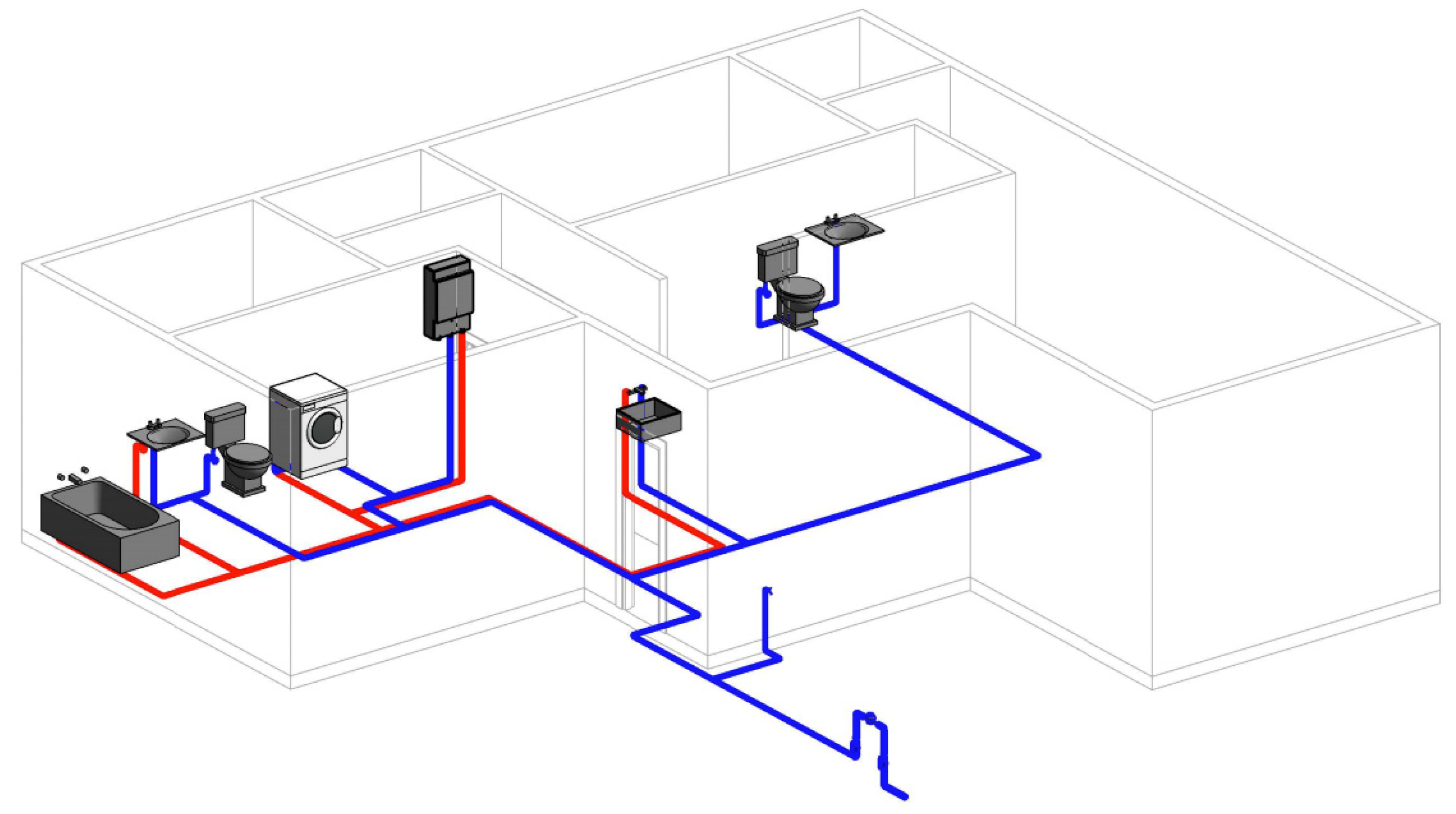
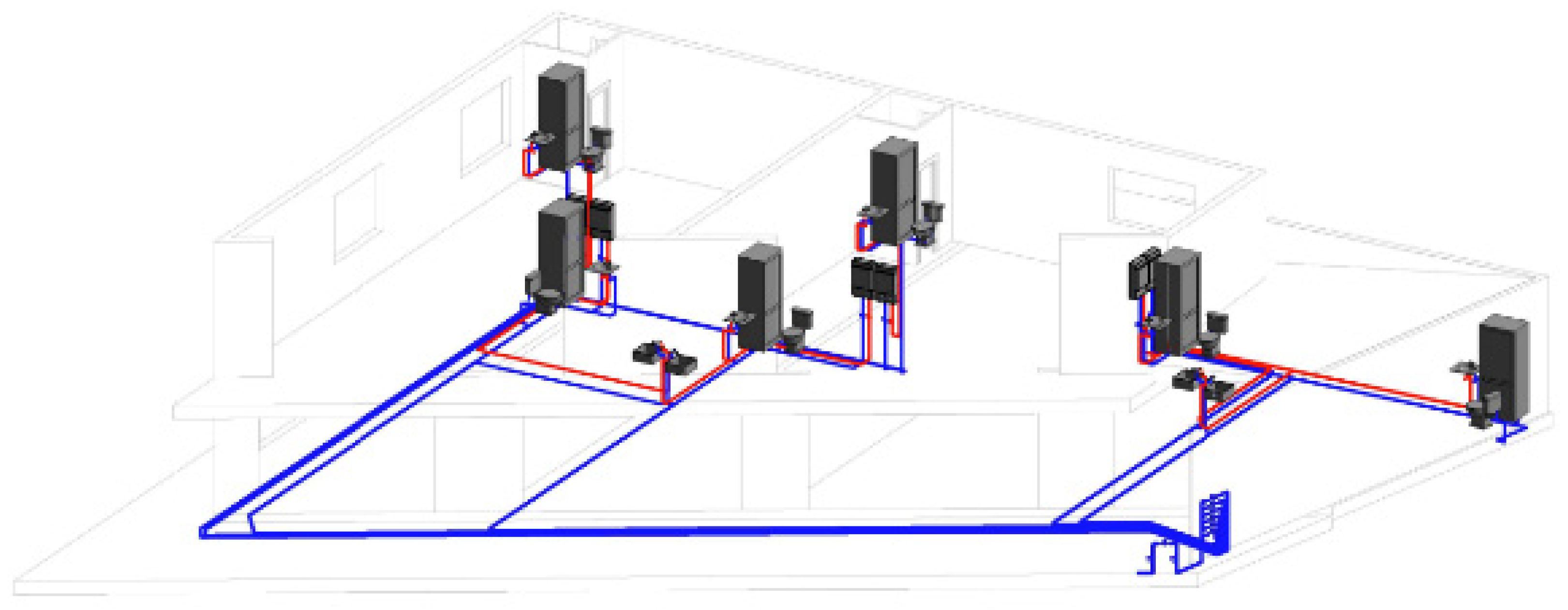
The presentation of a project includes various documents and outputs for each of the systems to be designed, commonly involving the use of floor plans, detail drawings and calculation tables. However, the features and capabilities of BIM tools allow all these documents to be stored in a single model, enabling the stored information to be updated in real-time and, thus, reducing the amount of repeated work required if changes must be made to the project [36]. Two types of templates were thus created to export the BIM models within Autodesk® Revit®. In the case of sanitary plumbing networks, the plan views of each floor of the structure were shown separately, with separate floors for the cold-water and hot-water systems. On the other hand, for the drainage networks, the template showed the floor plan view of each floor and the floor plan view of the manholes, together with information on the hydraulic equivalent units (HEUs, a quantification of the wastewater discharge generated by each fixture with reference to the RIDAA) and the slope corresponding to each pipe (Figure 3).

5. Case Study

This section describes the methods used for the case studies and the results obtained from the automation processes. Section 5.1 shows the results associated with drinking-water systems, including the hot- and cold-water networks. Section 5.2 shows the results of the automation for sewerage systems.

5.1. Drinking-Water System Calculation

A series of tables with numerical information associated with the parameters involved in the regulations for sanitary plumbing networks were created as a starting point for the calculation processes [26]. These values are not subject to variation since the formulations and design methods have not undergone significant modifications, so they can be considered as fixed input data for any type of project.
The acronyms established for the denomination of sanitary fixtures were based on the RIDAA and are shown in Table 2.
In some cases, values were adapted to optimise automatic calculation processes and avoid erroneous criteria related to network sizing, consumption and the calculation of pressure losses. The values provided by the RIDAA are organised according to the range of endowments in single-family housing or “dwelling house”-type structures, which can fluctuate between 80 and 450 L/inhab/day, according to the regulation. In our case, the minimum starting value was rounded to 250 L/inhab/day, taking as a reference the regulatory minimum of 211.6 L/inhab/day. These values are related to the Chilean average residential drinking water consumption and take into consideration the fact that any housing unit will have at least one bathroom (including a toilet, bathtub and sink), a kitchen and a washing machine [39]. This value rises as the number of bathrooms in the network increases, as shown in Table 3. For practical purposes, the term “medium” is used for bathrooms that do not have a bathtub or rain bath; in other words, those which contain only a sink, a toilet and possibly a bidet.
For the water-meter calculation, the regulation indicates that the maximum admissible head loss is 5 mca (meters of water column). This value is calculated according to the maximum probable flow rate, which is obtained from the fixtures’ consumption rates, and the maximum daily consumption rates, obtained according to the building’s supply and occupancy. However, since the networks studied are directly connected to the public network (without storage tanks or elevation mechanisms), they are limited to only the maximum probable consumption. The tabulated maximum daily consumption rates (Table 3) only represent reference values [26]. For this reason, the actual value of the maximum daily consumption should be used only when the resulting loss in the meter is less than 5 mca. Otherwise, the maximum daily consumption rate corresponding to the meter diameter that complies with the probable maximum flow rate, as indicated in Table 4, can be used to calculate the losses.
In the case in which a network has sub-meters with diameters that are not consecutive values in relation to the general meter diameter, according to the order tabulated in Table 4, the final diameter of the sub-meter should be considered as the value immediately below the diameter of the general meter of the system. This is for construction purposes because, if diameters differ by more than two values, the connection of the meter to the sub-meter segment would lead to the incorporation of an unnecessary number of diameter reduction accessories, making the sub-meter inefficient in terms of construction.
The material type of the pipe is defined according to the minimum acceptable nominal pressure for water conduction, which must be greater than or equal to 10 kgf/cm2 [26]. In addition, the usable diameter is limited to a minimum, imposed by the RIDAA, of 13 mm for copper or 16 mm for plastic materials. In addition, diameters that are not commercially available are not considered, as is the case for 15 mm copper pipes.
Based on the parameters required as input data for the calculation of sanitary plumbing networks, as well as the considerations previously mentioned, a database spreadsheet was generated. The contents of this spreadsheet are summarised in Table 5.
As an adaptation for the automatic iteration processes, and in order to obtain results within the normative margins, a safety criterion can be established regarding the flow velocities in the pipes for the conduction of drinking water. The maximum flow velocity must be 2.5 m/s for external or main distribution pipes and 2.0 m/s for the internal pipes of the network [26]. As a result, the restriction limiting velocity can be modified to 2.0 m/s in all the pipes of the system, regardless of their conditions, except for the section located immediately downstream of the house connection, where the restriction can be maintained at 2.5 m/s. These values are selected under the assumption that this section will be the one with the largest diameter in the entire network. This definition has the purposes of giving continuity to the changes in diameter between the different sections and protecting the system from possible damage due to water hammer effects.
Applying the workflow described in Figure 2, different series of codes were analysed and tested in order to extract the relevant information from the model. The optimal and lightest way to transfer the data corresponding to each object in the project model in an organised and accurate way was sought. The process obtained after applying the workflow is shown in Figure 4.
Figure 4 shows the process, which contains five steps, for the automation of the calculation of sanitary plumbing systems. Each step is composed of activities. The activities, supported by parametric programming with Dymamo, are related to the number of scripts used, which contain the programming code. These scripts are available in Appendix A to allow for the replication of the process and are as follows. (1) BIM modelling: this step is carried out with the software Revit and enables the location of the sanitary plumbing facility and the system’s network. (2) Parametric programming: the Dynamo parametric tool is used to identify the different systems and their quantities, as well as to obtain the critical path of the systems. All systems’ components are sorted according to the critical path and exported to a spreadsheet. (3) Calculations: The information obtained by Dynamo is organised in tables and exported to a database in the software Excel. In this software, iterative calculations are carried out to achieve compliance with the design standards until the final design parameters are obtained. (4) Parametric programming: the Dynamo tool is used to transfer the information in Excel to Revit. (5) Updating the BIM model: the final MEP model, along with the required data, is updated in Revit with the information from Dynamo.

5.1.1. Drinking-Water System Calculation—Case Study 1

The designed house has the basic appliances for a structure of this type distributed on a single floor. It is assigned an occupancy of five habitants and a garden area of 20 m2. As mentioned in Section 4.1, the input parameters incorporated by the user correspond to the preliminary layout of the drinking water and sewerage networks and the global characteristics of the project. Figure 5 shows the 3D model created with Autodesk® Revit®, where the fixtures and cold-water, hot-water and drainage networks are identified. Table 6 details the global project data in accordance with the requirements of Chilean regulations.
The second step of the process is the insertion of the preliminary information for the project into the project information chart, as shown in Table 6 and Figure 6.
Once the information for the architectural model has been complemented with the manual routing and the general information for the project, it is necessary to ensure the correct modelling of the connections between pipes and fixtures so that the data will not present errors resulting from manual routing. Then, script 1 and script 2 from Dynamo are executed, which extract and order the information, identify the fixed and variable parameters for the design, group them and create nodes that determine the pipe sections and their connections in order to determine of the critical route of the system. This information assigns names to the systems and nodes (through scripts 3 and 4). Figure 7 shows the result of the identification of the nodes and systems within the structure.
The information generated and extracted from the model is inserted into the spreadsheet. Each system present in the house (cold water and hot water) is differentiated and the information is sorted according to the entities derived from the 3D model. Figure 8 shows the distribution of the information in the parameter insertion spreadsheet.
The information is then processed using automatic iterative formulations in MS Excel®, modifying the diameter of each pipe section until a value that complies with the minimum standards of the regulation and the previously adopted criteria is obtained (Table 4).
As a result, the data corresponding to the tables for the total flow rates of the fixtures contained in the house (Table 7) and for the calculation of the meter (Table 8) are obtained.
The diameter of and losses in the drinking water-meter can be calculated similarly. According to Table 9, the actual maximum daily consumption is not high enough for the pressure losses to be less than 5 mca. Therefore, the consumption corresponding to the 19 mm meter, obtained from Table 4 with the probable maximum flow, is automatically assigned, resulting in a pressure loss that complies with the regulations.
Table 9 shows the losses in the cold-water network of the house, summarising the results subject to restrictions and improving the general visualisation of the values.
Table 10 summarises the losses corresponding to the hot-water network of the house.
As shown in Table 7, the developed algorithm allows the fixtures present in the system to be identified and assigns the acronyms used for their abbreviation in the tabulations. It interprets the connections of the appliances to the hot- and cold-water systems in order, finally, to calculate the values of the final and total flow rates installed in the house. As shown in Table 9, the flow velocity values comply with the maximum of 2.0 m/s, even in the first section. Likewise, all the final pressures of the system comply with the required minimum of 4 mca. The diameters show a downward variation but maintain a value of 13 mm in the sections connected to the fixtures. In addition, the calculation table is ordered starting with the critical path from the meter to the most unfavourable device, which in this case is the rain bath (BOLL). Since there is only one floor in the house, this is the point of highest elevation in the entire system. In the hot-water system, the flow rates and final pressures satisfy the regulatory restrictions. As shown in Table 10, the initial section (CAL-I) starts at the heating device (CAL), so the initial pressure is not equal to the 14 mca coming from the meter but to the pressure resulting from the section that ends at the heater, indicated in Table 9 (H-CAL).
Based on the results obtained for the single-family-house case, it is possible to verify the correct performance of the algorithms in terms of their effective recognition of the devices and maintenance of the desirable diameters (in the case of copper pipes, 13 mm) in the sections they are present in. In addition, algorithms demonstrated the ability to perform iterative calculations of diameters progressively until the minimum pressures are met, and the calculation criteria were correctly followed along the critical path.

5.1.2. Drinking-Water System Calculation—Case Study 2

The second case study represents a real project, previously designed and with values calculated using the traditional methods described in Section 3.1 and approved by the DDWSS local administration. The building is structured over two floors and contains six retail stores inside the building and a garden area of 20 m2. Each store has a water sub-meter fed from a general water meter. In addition, it has a 200 L/min wet fire suppression network. This project belongs to the category “commercial or office premises”, so its occupancy is measured in terms of its surface area. Figure 9 shows the 3D model of the project, which is based on interpretation of the CAD drawings. Table 11 summarises the global data for the project.
The architecture was designed with two different retail store patterns: those on the second floor have one less fixture than those on the first floor. Therefore, two different cases were considered for the study, choosing the stores on each floor that are farthest from the drinking water meter, as these are the most unfavourable in terms of friction losses due to the greater length of their pipes. Retail store type 1 has a toilet, sink, dishwasher and rain bath, while retail store type 2 has a toilet, sink and dishwasher. Figure 10 shows the systems for each of the types of stores used for the study.
As in the case of the single-family house, the information corresponding to the general characteristics of the building is incorporated into a chart (Figure 11).
With the information from the architectural model, scripts 1 and 2 are executed in Dynamo to obtain the nodes and sections of each system present in the structure, assign names to them (scripts 3 and 4) and determine the critical path. Figure 12 shows the results of the identification of the nodes and systems within the structure.
As in the first case, the information is inserted into the MS Excel® spreadsheet. The results for the second case study are presented as follows. The general table of installed loads in the system is shown in Table 12, and the calculation memory of the drinking water meter that feeds the entire system is shown in Table 13.
As mentioned above, calculations for the networks were undertaken for two types of retail stores, which are representative of the configurations found in the project. Thus, we can begin by showing the results for the type 1 store. Table 14 shows the flow rate chart.
As for the previous building, the contributions of the fixtures to the system were identified and quantified, and the total installed flow was calculated.
Once the system flow rates were determined, the calculation for the water sub-meter associated with the retail store was performed, yielding the results shown in Table 15.
Table 16 shows a summary of the losses chart for the type 1 retail store.
Table 17 shows the summary of hot water network losses.
The flow rate table corresponding to the type 2 store in the retail store project is shown in Table 18.
As previously, the resulting values for the installed flow rates were correctly obtained, counting the fixtures with cold and hot water. In this case, a lower value for the total flow is evident due to the lower number of fixtures in this system. The result for the corresponding sub-meter is shown in Table 19. The table of losses for the type 2 retail store is shown in Table 20.
As a final result, the loss table for the hot-water network of the store under analysis is shown in Table 21.
The results of the automatic export of the results are presented in Figure 13. The obtained data are compiled in a standard plan, displaying views of the structure together with the tables corresponding to the installed flow rates, head losses and meter and sub-meter calculations. This plan is based on the technical format imposed by the RIDAA, whereby the detailed drawings of the meter niche, sub-meters, starter and boiler device are included, resulting in a format ready to be presented in an application for sanitary service feasibility evaluation.

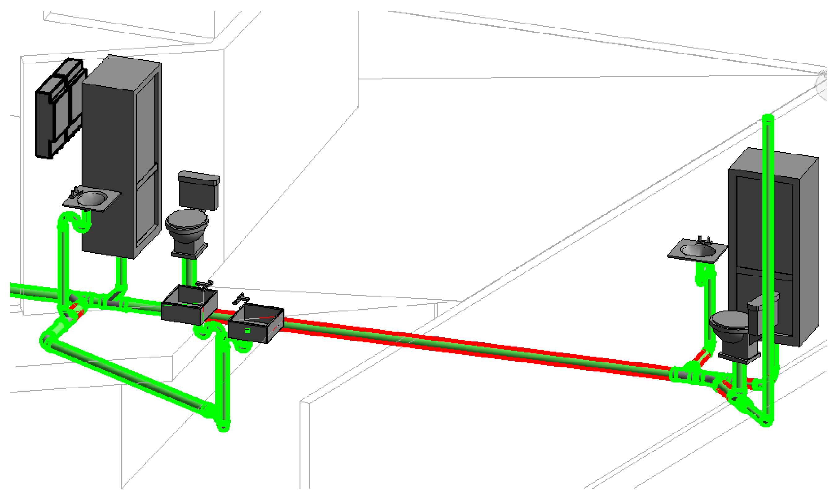
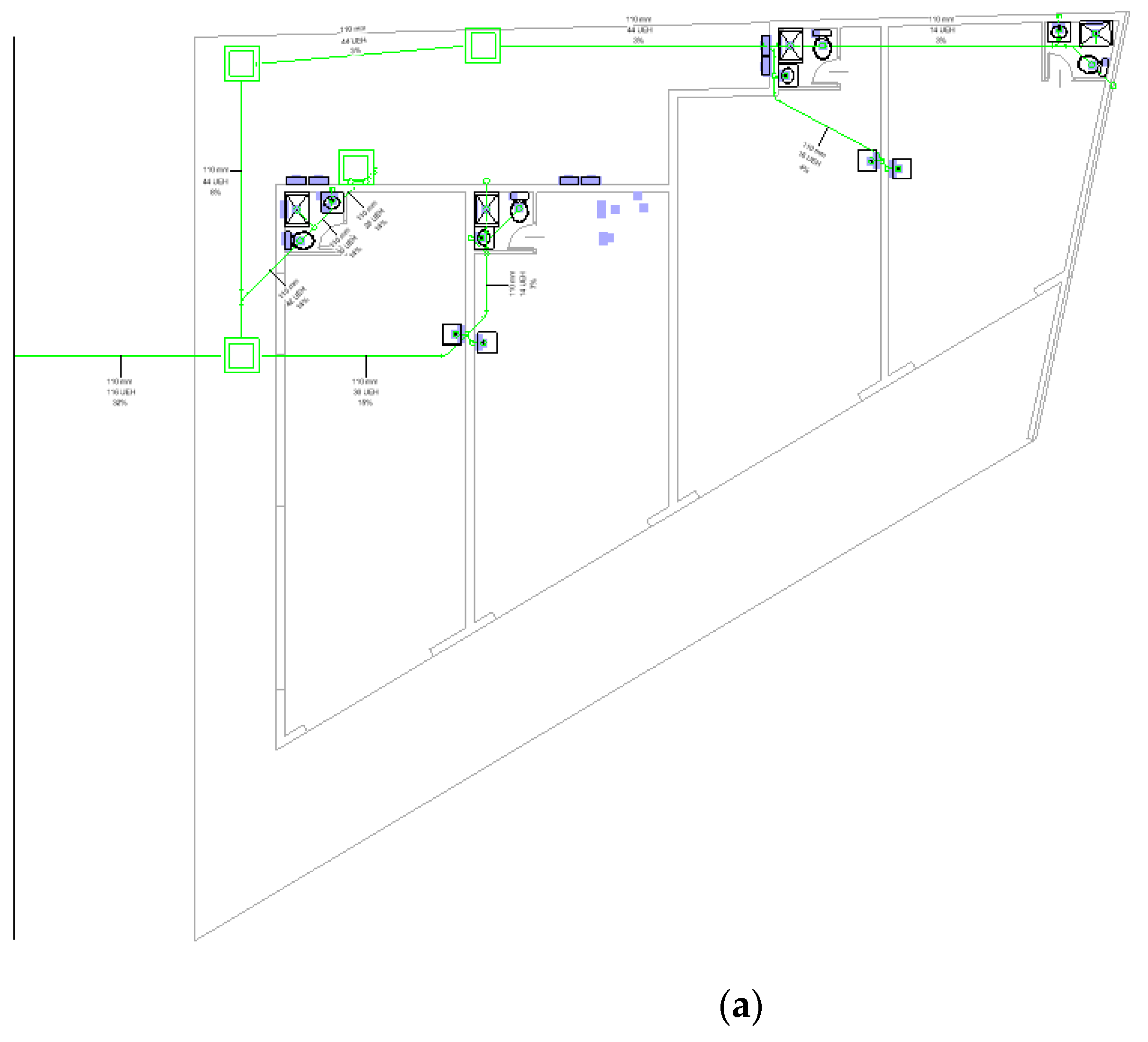
5.2. Sewage System Calculation

The sewerage network implementation methodology starts with a similar approach as for drinking water networks. Modelling considerations for sanitary drainage must cover all implications of gravitational flow. As defined in traditional methods and by code requirements, system routing must be constructed to ensure continuous operation and discharge of waste flow. The modelling process starts by assigning all plumbing fixtures a discharge route and assigning pipe segments throughout the construction plan, from the fixture outlets to the public collector, assuming initial slopes match the minimum values allowed by regulations. Manhole positioning must then be considered when routing pipes, as they must be placed on the outer part of the building and ensure continuity for every discharge.
Three-dimensional model geometry data information and parameters are extracted from plumbing fixtures and piping elements. This model is obtained by generating a system grouping and filtering according to sanitary classifications, at which point the relevant data are stored and distributed for further analysis. All drainage system piping elements are taken downstream from each fixture discharge sequentially, with the exception of manholes, as defined by the flow direction. This system is described in terms of the HEUs that every pipe must discharge in accordance with [26]. The application of the workflow described in Figure 2 for a sewerage system is detailed in Figure 14.
Figure 14 shows the sewerage system process verification. This process is composed of three steps. Each step is also composed of activities. The activities, supported by Dynamo, are related to the number of scripts used, which contain the programming code. These scripts are available in Appendix A to allow for the replication of the process and are as follows. (1) BIM modelling: this step, undertaken in Revit, involves the sewerage system layout and fixture description. (2) Parametric programming: Dynamo software is used to calculate the discharge slopes and pipe diameters in a first design. This design is divided into different pipes and sections in order to carry out the verification according to the design standard. (3) Verification: after the second step, two messages may be displayed. On the one hand, if issues (such as non-compliance with minimum and maximum slopes) are identified, a message is presented to the user requesting manual correction. On the other hand, if there are no issues to correct, a message stating “no issues” is displayed.
The objects or pipes assigned to each plumbing fixture extracted in the previous nodes are separated into sub-lists, in which each waste flow value is assigned according to sub-list indexes. The pipe positioning determines whether a single element is included in several different-sub lists and received discharges or waste flow from multiple fixtures. This allows the detection and determination, using summary functions, of the total discharge units for each pipe according to their repeated display in sub-lists and their HEU values. The obtained values are loaded into the element parameters of each pipeline. This is achieved by indicating the element instance, the parameter name and the new values. In addition, tagging pipe elements and calculating HEU values also provides relevant code-referenced information. This allows differentiation between pipes that contain streams from a single or multiple artefacts, called “secondary pipelines” and “primary pipelines”, respectively (RIDAA). This procedure can also be applied in order to identify ventilation system elements (Figure 13, script 8), where the flow value must be equal to zero because they do not have any relationship with any fixture upstream of their components, as shown in Figure 15.
Regular design codes for house sewerage systems describe a verification-based methodology for network calculation. This involves establishing limits or variation ranges for design parameters, such as diameters, slopes, fitting angles, elevation and HEUs. This approach enables alignment for validation tests through database integration directly into the Dynamo workflow, without requiring external software connections or data transfer. Each verification table is referenced and explained in code documents for sewerage calculations, including its application form and limitations. Tables are changed into Dynamo nodes as a list, following the exact order shown in the code documents. These tables are organised after collecting all element parameters and associating and grouping geometry parameters, flow values and slopes into separated lists. They are then linked to verification tables through logic algorithms. The first verification ensures no diameter reduction between any plumbing fixture and its downstream discharges. Workflow criteria assume that the minimum discharge diameter of every fixture is uploaded as an element parameter, has been previously read and is stored in sub-lists. Piping elements from each fixture are uploaded and sorted according to the downstream flow into a list connected to a node that reads internal element diameters. The information obtained is compared with the minimum fixture discharge diameter and loaded into element parameters according to system routing and conditions (Figure 13, script 9).
The second verification requires all the information previously calculated and uploaded as element parameters. Where geometric pipe parameters are matched with their corresponding axes within verification tables, diameters and slopes are identified and compared in the tables’ rows and columns to obtain the maximum HEU value for each pipe. These tabulated values are also distinguished in terms of primary and secondary pipelines, indicating whether it is necessary to modify segment parameters. Such modifications must be performed by editing parameters manually.
However, it is difficult to easily modify lengths and slopes simultaneously since adjacent elements share position parameters, so modifying them may cause disconnections or invalidity in the internal mechanics of the systems. Therefore, minimum diameters can be changed automatically. If pipe slopes do not satisfy specified limit values, the algorithm highlights the pipe in a striking colour, so that users know which section presents normative problems (as shown in Figure 16). This algorithm thus allows model configurations to be manually re-designed and adjusted until the whole system complies correctly when the verification code is executed again (Figure 13, script 10).
A check is also made for pipes that exceed the tabulated slopes or the established maximum of 15%, as well as whether they have sufficient slopes to withstand the discharge conditions. Once these verifications are finished and the sizing design is developed, the final documentation needs to be generated to assign floor plans and isometric views to corresponding sheets and implement the code presentation format (Figure 17).

6. Results and Discussion

The developed workflow shows that several design activities can be automated. The interaction with DDWSS components makes it possible to simplify the algorithm’s development through data management and calculations with visual programming. As sanitary calculation requires flow analysis, Dynamo provides specified nodes that work especially well with plumbing facilities, correctly organising and detecting every system element and evaluating its properties [41]. Node customisation allows specific data storage for verifications, modifications and calculations. The case studies prove that different approaches can be developed to satisfy different user requirements, meaning that the proposed approach is a generalisable solution for sanitary design. The Dynamo-friendly user interface makes programming comfortable and intuitive; node-based tasks make smooth workflows easier to structure and connect between different actions.
The ability to manipulate data between different software packages helps designers integrate specific calculations and more complex analyses. DDWSS design requires several iterations and developing an optimised design requires a large-scale mechanical design that modelling software cannot handle.
For the drinking-water system design in case study 1, different pipeline systems were read or extracted upstream from each fixture. Elements were divided into sub-lists, and each one was labelled according to a given numeration stored in the sub-meter properties and element parameters. Each element was then associated with each system uploading a mark type, allowing differentiation of the elements that feed each room domain (Figure 4, script 1). Pipe sections were then differentiated according to fixture positioning on the respective system routing, locating “Tee” elements that distribute water flow to fixture water inlets. These were obtained by assigning each Tee node a letter or a number, ensuring clarity about each system sector and the ability to tabulate all necessary parametric information (Figure 4, script 2). The purpose of script 2 is to identify energy losses due to friction, as well as singular losses, changes in elevation, flow rates and velocities as the water is distributed, and calculate the pressure at each fixture. For better pipe section tabulation, the most critical artefact in the system is highlighted according to its available pressure. This starts with pipe sections that take the route to the artefact of the building that has the highest elevation—this is referred to as the critical route since it generally has the lowest pressure in the system. After that, the additional tranches are added (Figure 4, script 3). Once the general information for the project has been defined along with the discretisation and marking of all the pipe sections, the next step is to extract the data to an MS Excel® worksheet to facilitate the respective calculations. This follows the same order that was given for the critical route, and then follows the ensuing sections to the remaining artefacts (Figure 4, scripts 4 and 5).
The results for the second case study for the drinking-water system design (Table 12 and Table 13) demonstrate the design’s good performance in detecting the fixtures and re-calculating installed flow rates. For the loss summary for cold water in the type 1 retail store (Table 16), the speeds and pressures comply with the normative restrictions. The diameters maintain the pattern of decrease, except for the sections that end in a fixture. Table 22 shows the results obtained for diameters and pressures in each section, along with the results obtained with the traditional method.
The comparison of the values shows that the developed workflow produced similar results to the traditional design approach and performed correctly and in compliance with the RIDAA design standard. No trend can be observed with regard to the pressure results, as the variations were both positive and negative. The relative percentage error ranged from 0.09% to 7.12%. Part of this error could be related to the variability generated by modelling the project on the basis of two-dimensional floor plans (produced using CAD). Due to elevation changes, this variability cannot be completely interpreted, generating differences in elevation that can affect the accuracy of the final pressure calculations. The high level of craftsmanship involved in traditional methods could be another cause of this difference. However, the obtained results ensure—with regard to the design standard—operating conditions that have a certain safety factor established by rounding values, such as the maximum probable flow rate or the singular loss calculations. In addition, the difference may have been influenced by the criteria applied by the professional who performed the calculations for the project.
As for the cold-water network sections, the margins of losses and velocities are comparable to those of the hot-water network. Table 23 shows a comparison of the results with the known values.
In this case, the diameters of the actual project did not completely agree with those obtained through automation, since in the sections leading to an appliance, the criterion of maintaining the 13 mm diameter was assumed to simplify the connection with the outlet taps, avoiding the excessive use of fittings at the terminals of the network. However, using a 19 mm diameter does not represent a significant problem, since it is still an acceptable size for connecting a sanitary fixture. The larger diameter may have been associated with the rather conservative criterion applied by the professional responsible for the project. With regard to the final pressures, the error range varied between 3.08% and 13.03%, values higher than those calculated for the cold-water network. This variability could be associated in part with the difference in the determination of diameters, since larger diameters increase pressure in all the systems. Table 24 compares the actual and calculated results for diameters and pressure losses in the type 2 retail store.
There were no differences in the selected diameters, and the minimum diameter was maintained in the sections with artefacts. On the other hand, the relative errors showed extreme values throughout the network, with a minimum error of 0.58% and a maximum error of 20.04%. The latter value generated an underestimation of the network capacity, since using the automatic method resulted in a higher pressure being obtained in the affected section. Although this error was quite high compared to the actual result, the presented algorithm performed the calculations based on exact numerical information, implying more reliable and accurate results. It can thus be assumed that relative errors with high values suggest an inaccurate interpretation of the two-dimensional plans of the structure.
As shown in Table 18, and in comparison to the previous results, the maximum daily consumption was optimised, obtaining a head loss of 0.78 mca for a sub-meter of 25 mm. Finally, a comparison of the actual values and calculated values for pressure losses and diameters is shown in Table 25.
When looking at the diameters in Table 25, a clear difference in the first and third segments is evident. Again, this involved the use of larger diameters in the sections that lead to a fixture, as was the case for the “H-BOLL” section. As explained above, this difference was a result of the use of specific criteria for automation. Furthermore, in the case of the “CAL-G” segment, it can be inferred that the designer used a larger diameter in order to increase the pressure in the final segments of the network. However, the automated method shows that the accuracy in the calculation allows diameters to be reduced, as the value of the losses is known with greater reliability. Finally, the relative error with the highest value (22.87%) corresponded precisely to the increase in the load resulting from the use of larger diameters.
For sanitary drainage, the algorithm developed was able to realise the piping design correctly with regard to calculations, modifications and verifications; the performance of the software resulted in a reduction in the time taken to process information and display outcomes. Using programming to create verification tools requires more manual iterations, thus simplifying the project review process and reducing errors.
The scenarios described here assume a properly structured algorithm workflow; although Dynamo provides predefined nodes and simplified actions, building computational programming requires prior knowledge—not only about Dynamo itself but also about code –model interactions. Some of the difficulties found here are largely related to this factor. In some situations, element modifications carried out by automated tasks break connection rules, producing mismatches and separating the geometric and parametric correlation of elements.
Other errors are attributable to the use of MS Excel® in the data insertion stage; when working with lists separated by the system, data distribution must coincide with predefined sheet organisation. Otherwise, data packages can overwrite wrong cells, breaking the calculation logic and displaying incorrect results.
As indicated by the case studies, the proposed approach demonstrates that parametric modelling can host plumbing system attributes correctly, generating subsystems with accuracy and without missing or incorrect information during the modelling stage and parameterisation. However, some issues were found in the plumbing fixture selection: predefined elements contain parameters and calculations relating to international codes, and these calculations may need to be excluded, while local regulations may need to be integrated into Dynamo. Without a unified modelling and mechanical equipment standard based on BIM, some necessary data may be omitted, reducing the model accuracy and detail level.
Parametric design with visual programming helps designers in the early design stages, generating a process database that can be used to automate several actions and tasks. The application of these algorithms can be generalised, allowing users to understand their usage in diverse project topologies and obtain exact results if they provide their requirements consistently.

7. Conclusions

In this research, a BIM-based designed workflow for a domestic drinking-water and sewerage system was developed using a semi-automatised design process. This was achieved through the application of a DRSM. This development was integrated with applications that are widely used in the AEC industry: Autodesk® Revit® and MS Excel®. The main advantages of these tools are their interoperability, their potential for customisation and the ease of visual programming.
This paper delivers the following contributions. First, it was found to be possible to adapt BIM tools for DDWSS design projects while taking local standards into account (in this case, Chilean standards). Moreover, this research demonstrates a possible extension of BIM applications over and above typical uses, such as system coordination, clash detection and documentation generation.
The obtained workflow covers a wide part of the design process from an end-to-end perspective: starting with an initial 3D model and a DDWSS draft and proceeding to the designed and validated components displayed in the standardised templates established by the local authority, ready for the request for permission to begin construction. The tool developed, in addition to facilitating the design process by automating many of the tasks involved in it, allows similar results to be obtained to those obtained by the traditional method. Furthermore, the developed workflow reduces subjectivity and errors in the design process by concentrating all design rules and required verification procedures in the code. Therefore, the exploitation of this tool would also help to improve productivity in engineering offices.
Both the DSRM and the workflow obtained allow replication of this automation process in other contexts, so it is hoped that this work will encourage other researchers to expand the uses of BIM (and BIM tools). Moreover, the workflow obtained is suitable for moderately complex developments, as is the case for one- or two-story houses and systems without mechanical equipment, such as pumps. However, the software tools used have the advantage of allowing code customisation, opening the possibility of addressing more complex design scenarios in future studies.
Future studies could also expand knowledge about automatic programming to deal with class detection problems (also known as high and soft collision [42]). These problems increase in complex projects with several disciplines involved. Nowadays, various commercial solutions (such as Navisworks [42], Synchro [43] or Solibri [44]) are among the most efficient clash detection tools. An alternative or complement to these software packages is the use of parametric programming tools. For example, specific Dynamo nodes (such as Bymorph Nodes [45]) can improve the automation of the clash detection process. The integration of these protocols with the DDWSS problems presented in this study will be studied by the authors in future work.
Finally, this approach will hopefully motivate researchers and practitioners to make the design process easier by using BIM automation tools, such as Dynamo scripts, to bridge the digital divide in the AEC industry and maximise the advantages that BIM brings to engineering.

Author Contributions

Conceptualisation, P.A., F.O. and E.A.; methodology, P.A., F.O., E.A., F.M.-L.R. and R.F.H.; software, P.A. and F.O.; formal analysis, P.A., F.O., E.A., F.M.-L.R. and R.F.H.; writing—original draft preparation P.A. and F.O.; writing—review and editing, E.A., F.M.-L.R., R.F.H. and F.L.-G.; visualisation, P.A., F.O. and F.M.-L.R.; supervision, E.A., F.M.-L.R. and R.F.H.; funding acquisition, E.A. and F.L.-G. All authors have read and agreed to the published version of the manuscript.

Funding

This research was funded by Proyecto VRIEA-PUCV, grant number 039.427/2021, and the Grants for the Promotion of Research in the Department of Civil and Building Engineering, UCLM. This research was also funded by Spanish Ministry of Economy and Competitiveness provided through the research project BIA2013-47290-R, BIA2017-86811-C2-1-R and BIA2017-86811-C2-2-R. All these projects were funded with FEDER funds.

Institutional Review Board Statement

Not applicable.

Informed Consent Statement

Not applicable.

Data Availability Statement

Not applicable.

Acknowledgments

The authors wish to thank all organisations that participated in this study and the experts for the insight provided. The authors wish to thank the Technology, Innovation, Management, and Innovation (TIMS) space of the School of Civil Engineering of the Pontificia Universidad Católica de Valparaíso (Chile), where part of the research was carried out.

Conflicts of Interest

The authors declare no conflict of interest.

Appendix A

The files developed in this study are available at the following link for replication. The Revit models of the two case studies and the 10 scripts referenced in Figure 4 and Figure 14 are included. The spreadsheets with results are also included. Available online: https://drive.google.com/drive/folders/104TLNyzGZGcCBm7af3n23wJRLYO8l_XF?usp=sharing (Accessed on 8 September 2022).

References

  1. Abdelhameed, W.; Saputra, W. Integration of building service systems in architectural design. J. Inf. Technol. Constr. 2020, 25, 109–122. [Google Scholar] [CrossRef]
  2. Filho, J.B.P.D.; Angelim, B.M.; Guedes, J.P.; De Castro, M.A.F.; Neto, J.D.P.B. Virtual design and construction of plumbing systems. Open Eng. 2016, 6, 730–736. [Google Scholar] [CrossRef]
  3. Palomera-Arias, R.; Liu, R. BIM laboratory exercises for a MEP systems course in a construction science and management program. J. Inf. Technol. Constr. 2016, 21, 188–203. [Google Scholar]
  4. Zhang, J.; Seet, B.C.; Lie, T.T. Building information modelling for smart built environments. Buildings 2015, 5, 100–115. [Google Scholar] [CrossRef]
  5. Diao, P.H.; Shih, N.J. BIM-based AR maintenance system (BARMS) as an intelligent instruction platform for complex plumbing facilities. Appl. Sci. 2019, 9, 1592. [Google Scholar] [CrossRef]
  6. Loyola, M. Encuesta Nacional BIM 2019; Universidad de Chile-Plan BIM: Santiago, Chile, 2019. [Google Scholar]
  7. Peffers, K.; Tuunanen, T.; Gengler, C.E.; Rossi, M.; Hui, W.; Virtanen, V.; Bragge, J. The Design Science Research Process: A Model for Producing and Presenting Information Systems Research. In Proceedings of the 1st International Conference, DESRIST 2006 Proceedings, Claremont, CA, USA, 24–25 February 2006; Claremont Graduate University: Claremont, CA, USA; pp. 83–106. Available online: http://urn.fi/URN:NBN:fi:jyu-201904092111 (accessed on 8 September 2022).
  8. SISS Domestic Drinking Water and Sewerage Systems Chilean Standard Catalog. Available online: https://www.siss.gob.cl/586/w3-article-4152.html (accessed on 8 September 2022).
  9. Xie, H.; Tramel, J.M.; Shi, W. Building information modeling and simulation for the mechanical, electrical, and plumbing systems. In Proceedings of the 2011 IEEE International Conference on Computer Science and Automation Engineering, Shanghai, China, 10–12 June 2011; Volume 3, pp. 77–80. [Google Scholar] [CrossRef]
  10. Xiao, Y.Q.; Li, S.W.; Hu, Z.Z. Automatically generating a MEP logic chain from building information models with identification rules. Appl. Sci. 2019, 9, 2204. [Google Scholar] [CrossRef]
  11. Wang, B.; Yin, C.; Luo, H.; Cheng, J.C.P.; Wang, Q. Fully automated generation of parametric BIM for MEP scenes based on terrestrial laser scanning data. Autom. Constr. 2021, 125, 103615. [Google Scholar] [CrossRef]
  12. Wang, J.; Wang, X.; Shou, W.; Chong, H.Y.; Guo, J. Building information modeling-based integration of MEP layout designs and constructability. Autom. Constr. 2016, 61, 134–146. [Google Scholar] [CrossRef]
  13. Chen, Q.; García de Soto, B.; Adey, B.T. Construction automation: Research areas, industry concerns and suggestions for advancement. Autom. Constr. 2018, 94, 22–38. [Google Scholar] [CrossRef]
  14. Muñoz-La Rivera, F.; Vielma, J.C.; Herrera, R.F.; Carvallo, J. Methodology for Building Information Modeling (BIM) implementation in structural engineering companies (SECs). Adv. Civ. Eng. 2019, 2019, 8452461. [Google Scholar] [CrossRef] [Green Version]
  15. Teng, Y.; Xu, J.; Pan, W.; Zhang, Y. A systematic review of the integration of building information modeling into life cycle assessment. Build. Environ. 2022, 221, 109260. [Google Scholar] [CrossRef]
  16. Herrera, R.F.; Morgues, C.; Alarcón, L.F.; Pellicer, E. Analyzing the association between lean design management practices and BIM uses in the design of construction projects. J. Constr. Eng. Manag. 2021, 147, 1–11. [Google Scholar] [CrossRef]
  17. Leygonie, R.; Motamedi, A.; Iordanova, I. Developments in the built environment development of quality improvement procedures and tools for facility management BIM. Dev. Built Environ. 2022, 11, 100075. [Google Scholar] [CrossRef]
  18. Collao, J.; Lozano-galant, F.; Lozano-galant, J.A. BIM Visual programming tools applications in infrastructure projects: A state-of-the-art review. Appl. Sci. 2021, 11, 8343. [Google Scholar] [CrossRef]
  19. Žurić, J.; Zichi, A.; Azenha, M. Integrating HBIM and sustainability certification: A pilot study using GBC historic building certification. Int. J. Archit. Herit. 2022, 1–20. [Google Scholar] [CrossRef]
  20. Potrč Obrecht, T.; Röck, M.; Hoxha, E.; Passer, A. BIM and LCA integration: A systematic literature review. Sustainability 2020, 12, 5534. [Google Scholar] [CrossRef]
  21. Ren, R.; Zhang, J. A new framework to address BIM interoperability in the AEC domain from technical and process dimensions. Adv. Civ. Eng. 2021, 2021, 8824613. [Google Scholar] [CrossRef]
  22. Bastos Porsani, G.; de Lersundi, K.; Sánchez-Ostiz Gutiérrez, A.; Fernández Bandera, C. Interoperability between building information modelling (BIM) and building energy model (BEM). Appl. Sci. 2021, 11, 2167. [Google Scholar] [CrossRef]
  23. Bellido-montesinos, P.; Lozano-galant, F.; Javier, F.; Lozano-galant, J.A. Experiences learned from an international BIM contest: Software use and information work fl ow analysis to be published in: Journal of Building Engineering. J. Build. Eng. 2019, 21, 149–157. [Google Scholar] [CrossRef]
  24. Xie, X.; Zhou, J.; Fu, X.; Zhang, R.; Zhu, H.; Bao, Q. Automated rule checking for MEP systems based on BIM and KBMS. Buildings 2022, 12, 934. [Google Scholar] [CrossRef]
  25. García, D. Aplicacion de BIM a Instalaciones Hidráulicas en Edificacion; Universidad de Valladolid: Valladolid, Spain, 2019. [Google Scholar]
  26. Ministerio de Obras Públicas de Chile. Reglamento de Instalaciones Domicliarias de Agua Potable y Alcantarillado (RIDAA); Biblioteca del Congreso Nacional de Chile: Santiago, Chile, 2009. [Google Scholar]
  27. Council, I.C. International Plumbing Code; ICC: Washington, DC, USA, 2012; ISBN 9781580017428. [Google Scholar]
  28. CNP. Productividad en el Sector de la Construcción; Santiago de Chile: Santiago, Chile, 2020. [Google Scholar]
  29. Lu, Q.; Wong, Y.H. A BIM-based approach to automate the design and coordination process of mechanical, electrical, and plumbing systems. HKIE Trans. 2018, 25, 273–280. [Google Scholar] [CrossRef]
  30. Han, J.; Zhou, X.; Zhang, W.; Guo, Q.; Wang, J.; Lu, Y. Directed representative graph modeling of MEP systems using BIM data. Buildings 2022, 12, 834. [Google Scholar] [CrossRef]
  31. Wei, T.; Chen, G.; Wang, J. Application of BIM technology in water supply and drainage design. In Proceedings of the IOP Conference Series: Earth and Environmental Science; IOP Publishing: Bristol, VA, USA, 2017. [Google Scholar]
  32. Kalasapudi, V.S.; Turkan, Y.; Tang, P. Toward automated spatial change analysis of MEP components using 3D point clouds and as-designed BIM models. In Proceedings of the 2014 2nd International Conference on 3D Vision, Tokyo, Japan, 8–11 December 2014; pp. 145–152. [Google Scholar] [CrossRef]
  33. Hu, Z.Z.; Yuan, S.; Benghi, C.; Zhang, J.P.; Zhang, X.Y.; Li, D.; Kassem, M. Geometric optimization of building information models in MEP projects: Algorithms and techniques for improving storage, transmission and display. Autom. Constr. 2019, 107, 102941. [Google Scholar] [CrossRef]
  34. Pärn, E.A.; Edwards, D.J.; Sing, M.C.P. Origins and probabilities of MEP and structural design clashes within a federated BIM model. Autom. Constr. 2018, 85, 209–219. [Google Scholar] [CrossRef]
  35. Vasilev, L. Parametric Modeling in Structural Design. Thesis, LAB University of Applied Sciences, Lahti, Finland, 2020. Available online: https://www.theseus.fi/bitstream/handle/10024/349329/Parametricmodelinginstructuraldesign.pdf?sequence=2 (accessed on 8 September 2022).
  36. Stine, D. Autodesk Revit for Architecture Certified User Exam Preparation; SDC: Nashville, TN, USA, 2021. [Google Scholar]
  37. Jezyk, M. Dynamo Primer guide. Available online: https://primer.dynamobim.org/ (accessed on 8 September 2022).
  38. Wei, L.; Liu, S.; Wei, Q.; Wang, Y. Concept, method and application of computational BIM. Adv. Intell. Syst. Comput. 2020, 1084, 392–398. [Google Scholar] [CrossRef]
  39. Hofmann, P.; Samp, C.; Urbach, N. Robotic process automation. Electron. Mark. 2020, 30, 99–106. [Google Scholar] [CrossRef]
  40. Parti, R.; Hauer, S.; Monsberger, M. Process model for BIM-based MEP design. IOP Conf. Ser. Earth Environ. Sci. 2019, 323, 012045. [Google Scholar] [CrossRef]
  41. Nezamaldin, D. Parametric Design with Visual Programming in Dynamo with Revit: The Conversion from CAD Models to BIM and the Design of Analytical Applications. Master’s Thesis, Royal Institute of Technology, Stockholm, Sweden, 2019; 84p. [Google Scholar]
  42. Hu, Y.; Castro-Lacouture, D.; Eastman, C.M. Holistic clash detection improvement using a component dependent network in BIM projects. Autom. Constr. 2019, 105, 102832. [Google Scholar] [CrossRef]
  43. Ciribini, A.L.C.; Ventura, S.M.; Paneroni, M. Implementation of an interoperable process to optimise design and construction phases of a residential building: A BIM Pilot Project. Autom. Constr. 2016, 71, 62–73. [Google Scholar] [CrossRef]
  44. Merschbrock, C.; Erik, B. Effective digital collaboration in the construction industry—A case study of BIM deployment in a hospital construction project. Comput. Ind. 2015, 73, 1–7. [Google Scholar] [CrossRef]
  45. Autodesk Bymorph Nodes for Dynamo BIM. Available online: https://bimorph.com/bimorph-nodes/ (accessed on 2 September 2022).
Figure 1. Research methodology workflow.
Applsci 12 09063 g001
Figure 2. Workflow for drinking-water system (white boxes) and sewerage (grey boxes) design automation.
Applsci 12 09063 g002
Figure 3. Reference format for the exported plans.
Applsci 12 09063 g003
Figure 4. Activity sequence for automatic calculation of sanitary plumbing systems organised into five steps: (1) BIM modelling, (2) parametric programming, (3) calculations, (4) parametric programming and (5) updating BIM model. All the scripts are presented as Appendix A.
Applsci 12 09063 g004
Figure 5. Sanitary plumbing network layout in a single-family house.
Applsci 12 09063 g005
Figure 6. Project information chart for single-family house.
Applsci 12 09063 g006
Figure 7. Results after the application of scripts 3 and 4: (a) node identification and (b) sanitary plumbing system recognition.
Applsci 12 09063 g007
Figure 8. Insertion of the information for the pipes in an MS Excel® spreadsheet using scripts 5 and 6.
Applsci 12 09063 g008
Figure 9. Sanitary plumbing network layout for retail stores and offices.
Applsci 12 09063 g009
Figure 10. Sanitary plumbing water systems for the retail stores under study: (a) type 1 (first floor); (b) type 2 (second floor).
Applsci 12 09063 g010
Figure 11. Project information chart for a retail building.
Applsci 12 09063 g011
Figure 12. Results of the application of scripts 3 and 4: (a) identification of nodes with the assignment of letters; (b) recognition of the drinking-water network system.
Applsci 12 09063 g012
Figure 13. Presentation of the final results in standard layout format.
Applsci 12 09063 g013
Figure 14. Processes for sewerage system verification organised into three steps: (1) BIM modelling, (2) parametric programming and (3) verification. All the scripts are presented in the Appendix A.
Applsci 12 09063 g014
Figure 15. Household drainage network layout in a single-family house.
Applsci 12 09063 g015
Figure 16. Example of an alert for pipelines that do not comply with the established minimum.
Applsci 12 09063 g016
Figure 17. Sewerage system floor plan, including calculated HEUs for each segment on the first story (a) and the second story (b).
Applsci 12 09063 g017aApplsci 12 09063 g017b
Table 1. Examples of studies using Autodesk software that deal with interoperability problems.
ReferenceAimModelling SoftwareVisual Programming
Language Software
[17]Facility managementRevit, SolibriDynamo
[18]State of the art reviewRevit, Robot, TricalcDynamo, Grasshoper
[19]HeritageRevitDynamo
[20]State of the art reviewRevit, Rhino, ArchicadDynamo, Grasshoper
[21]CoordinationRevit, Robot-
[22]Interoperability studyRevit, gbXML, IFCEnergyPlus engine
[23]State of the art reviewRevit, Archicad, IFCDynamo, Grasshoper
[15]State of the art reviewRevit, Rhino, ArchicadDynamo, Grasshoper
[19]State of the art reviewRevit, Solibri, ArchicadDynamo, Grasshoper
[24]MEPRevitDynamo
Table 2. Acronyms used for the design of artefacts based on the Chilean RIDAA standard.
Plumbing FixtureAbbreviation UsedPlumbing FixtureAbbreviation Used
TroughBEGlasswasherLC
BidetBIHandwasherLO
BathtubBODishwasherLP
Rain showerBOLLLaundryLV
Shower with perforated pipeBPDishwashing machineLVV
HeaterCALWashing machineMLV
Wet netGRHUrinalUR
Yard tap 13 (mm)LLJ13Urinal with perforated pipeURP
Yard tap 19 (mm)LLJ19ToiletWC
Table 3. Adapted supplies for automatic calculation.
Building TypeSubtypeEndowment
Social housingNot applicable70 Lt/inhab/day
Single-family houseWith one bathroom, a kitchen and a washing machine250 Lt/inhab/day
With two and a half bathrooms, a kitchen and a washing machine300 Lt/inhab/day
With two bathrooms, a kitchen and a washing machine350 Lt/inhab/day
With three bathrooms, a kitchen and a washing machine400 Lt/inhab/day
With more than three bathrooms, a kitchen and a washing machine450 Lt/inhab/day
Single-start apartment buildingNot applicable450 Lt/inhab/day
Apartment building with an independent meter or sub-meterNot applicableEndowment varies by department and according to the subtypes applied for single-family dwellings
Commercial or office premisesOccupation per employee150 Lt/inhab/day
Occupancy by surface area10 Lt/m2/day
Bar, restaurant, fountain and similarNot applicable40 Lt/m2/day
Table 4. Table of meter capacities [26].
Diameter (mm)Maximum Daily
Consumption (m3/day)
Probable Maximum
Consumption (L/min)
13350
19580
257117
3820333
5030500
Table 5. Contents of the database for the calculation of sanitary plumbing water networks.
Type of DataPurposeAdaptations
Drinking water supply rangesMaximum daily consumption
calculation
Interpolated values of endowments in single-family dwellings are calculated according to the number of existing bathrooms
Accessory loss coefficientsSingular loss calculationNo adaptations
Pipe materials and diametersDetermination of frictional losses and flow velocityLimitations imposed by the regulations and the commercial diameters available in Chile
Consumption according to the type of sanitary applianceCalculation of installed and probable maximum flow ratesNo adaptations
Common artefact elevationsCalculation of elevation lossesAn average elevation is assumed based on architecture and depending on the type of artefact
Table 6. Global data for the single-family house case study.
Building TypeSubtypeNumber of
Occupants
Garden or Lawn SurfaceRecirculating Pool VolumePool Volume without
Recirculation
Firefighting Network
Single-family houseHouse with one and a half bathroomsFive residents20 m2000
Table 7. System flow rates table for a single-family house.
Plumbing FixtureAcronymPlumbing Fixture Supply (Lt/min)Cold Water
Quantity
Hot Water
Quantity
Supply (Lt/min)
ToiletWC102020
Yard tapLLJ13201020
HandwasherLO82124
BathtubBO151130
Washing machineMLV151130
DishwasherLP121124
Total installed flow (L/min)148
Table 8. Water-meter calculation report for a single-family house.
Water-Meter Calculation Report
System installed flow rate148.00 Lt/min
Maximum probable flow rate54.43 Lt/min
Meter diameter19.00 mm
Maximum daily consumption5 m3/day
Meter head loss4.27 mca
Table 9. Loss summary table for cold-water system in a single-family house.
SegmentMaterialTypeLength (m)Diameter (mm)Speed (m/s)Total Loss (mca)Final
Pressure (mca)
MAPACopperCu L2.19251.701.9212.08
ABCopperCu L3.40251.540.6911.40
BCCopperCu L3.52251.280.4210.98
CDCopperCu L2.93191.030.8610.12
DECopperCu L0.63190.800.0810.04
EFCopperCu L1.00190.600.049.99
FBOCopperCu L1.90131.253.176.83
ELOCopperCu L0.80130.811.278.76
DWCCopperCu L0.40130.940.779.35
CGCopperCu L0.93191.650.4710.50
GTCopperCu L1.26190.600.0610.44
TMLVCopperCu L1.10131.252.238.21
GHCopperCu L0.84191.370.1710.33
HCALCopperCu L1.40191.372.727.61
BPCopperCu L1.26190.970.1511.25
PRCopperCu L8.02190.680.3510.90
RSCopperCu L0.60190.450.0310.87
SWCCopperCu L0.40130.940.7510.12
RLOCopperCu L0.80130.811.309.60
PQCopperCu L1.64190.510.1911.06
QLPCopperCu L0.80131.071.599.46
ALLJ13CopperCu L0.60131.522.299.80
Table 10. Table summarising hot-water-system losses in a single-family house.
SegmentMaterialTypeLength (m)Diameter (mm)Speed (m/s)Total Loss (mca)Final Pressure (mca)
CALICopperCu L1.40191.37−0.377.98
IJCopperCu L1.05191.370.237.75
JOCopperCu L1.30190.600.067.69
OMLVCopperCu L1.10131.252.235.46
JKCopperCu L0.88191.070.167.59
KNCopperCu L6.31190.510.207.39
NLPCopperCu L0.80131.071.595.79
KLCopperCu L3.61190.800.267.33
LLOCopperCu L0.80130.811.276.06
LMCopperCu L1.00190.600.067.27
MBOCopperCu L1.90131.253.174.10
Table 11. Global data for the retail store building case study.
Building TypeSubtypeNumber of
Occupants
Garden or Lawn SurfaceRecirculating Pool VolumePool Volume without
Recirculation
Firefighting
Network
Commercial or office premisesOccupancy by surface area321.5 m220 m200200 Lt/Min
Table 12. Total installed loads chart for a commercial building.
Plumbing
Fixture
AcronymPlumbing
Fixture Flow Rate (Lt/min)
Cold Water
Quantity
Hot Water QuantityFinal Flow Rate (Lt/min)
ToiletWC106060
HandwasherLO86696
Rain showerBOLL1066120
DishwasherLP124496
Wet net200
Total installed flow (Lt/min)572
Table 13. General meter calculation report for a commercial building.
Meter Calculation Report
System installed flow rate572.00 Lt/min
Maximum probable flow rate138.13 Lt/min
Meter diameter38.00 mm
Maximum daily consumption20.00 m3/day
Meter head loss1.72 mca
Table 14. Flow rate table for type 1 retail store.
Plumbing
Fixture
AcronymPlumbing Fixture Flow Rate (Lt/min)Cold Water QuantityHot Water QuantityFinal Flow (Lt/min)
ToiletWC101010
HandwasherLO81116
Rain showerBOLL101120
DishwasherLP121124
Total installed flow (Lt/min)70
Table 15. Sub-meter calculation report for type 1 retail store.
Sub-Meter Calculation Report
System installed flow rate70.00 Lt/min
Maximum probable flow rate32.49 Lt/min
Sub-meter diameter25.00 mm
Maximum daily consumption7.00 m3/day
Sub-meter head loss0.78 mca
Table 16. Loss summary table for cold potable water system for type 1 retail store.
SegmentMaterialTypeLength (m)Diameter (mm)Speed (m/s)Total Loss (mca)Final Pressure (mca)
MAPRAPCopperCu L3.30251.020.7613.24
RAPACopperCu L2.56251.020.2113.03
ABCopperCu L28.39251.021.7611.27
BCCopperCu L2.20191.520.6010.68
CDCopperCu L0.99191.340.2910.39
DBOLLCopperCu L1.43130.942.158.24
DECopperCu L0.85191.140.2610.13
ECALCopperCu L1.72190.971.598.54
ELOCopperCu L1.46130.811.029.11
CWCCopperCu L0.67130.940.5710.11
BLPCopperCu L5.51131.071.679.61
Table 17. Loss summary table for hot potable water system, retail store type 1.
SegmentMaterialTypeLength (m)Diameter (mm)Speed (m/s)Total Loss (mca)Final Pressure (mca)
CALFCopperCu L1.19190.972.046.49
FGCopperCu L0.28190.970.156.35
GLOCopperCu L0.86130.810.975.37
GHCopperCu L1.33190.780.216.14
HBOLLCopperCu L1.18130.942.124.02
HLPCopperCu L8.19131.072.084.06
Table 18. Total installed loads chart for type 2 retail store.
Plumbing FixtureAcronymPlumbing Fixture Flow Rate (Lt/min)Cold Water QuantityHot Water QuantityTotal Flow Rate (Lt/min)
ToiletWC101010
HandwasherLO81116
Rain showerBOLL101120
Total installed flow (Lt/min)46
Table 19. Sub-meter calculation report for type 2 retail store.
R.A.P. Calculation Report
System installed flow rate46.00 Lt/min
Maximum probable flow rate24.33 Lt/min
Sub-meter diameter25.00 mm
Maximum daily consumption7.00 m3/day
Sub-meter head loss0.78 mca
Table 20. Losses in the cold potable water system for type 2 retail store.
SegmentMaterialTypeLength (m)Diameter (mm)Speed (m/s)Total Loss (mca)Final Pressure (mca)
MAPRAPCopperCu L11.93250.760.7313.60
RAPACopperCu L2.06250.760.1113.49
ABCopperCu L41.92250.761.5411.95
BCCopperCu L0.43190.923.328.63
CDCopperCu L3.16190.920.258.39
DECopperCu L0.33190.920.108.29
EFCopperCu L0.15190.680.058.24
FBOLLCopperCu L1.23130.942.136.11
FLOCopperCu L1.56130.811.037.21
EWCCopperCu L1.29130.940.677.61
BCALCopperCu L1.46190.681.5010.46
Table 21. Summary table for hot potable water system losses for type 2 commercial premises.
SegmentMaterialTypeLength (m)Diameter (mm)Speed (m/s)Total Loss (mca)Final Pressure (mca)
CALGCopperCu L3.16190.683.946.51
GHCopperCu L0.76190.680.096.42
HBOLLCopperCu L1.13130.942.124.30
HLOCopperCu L1.43130.811.025.40
Table 22. Comparison of diameters and final cold water pressure for type 1 retail store.
SegmentDiameter Using
Traditional Method (mm)
Diameter with Automation
(mm)
Final Pressure with Traditional Method (mca)Final Pressure with Automation (mca)Error between Pressure Results (%)
MAPRAP252513.7213.243.50%
RAPA252512.5713.033.66%
AB252511.1911.270.71%
BC191910.6910.680.09%
CD191910.5210.391.24%
DBOLL13138.058.242.36%
DE191910.3510.132.13%
ECAL19198.988.544.90%
ELO13139.059.110.66%
CWC13139.8010.113.16%
BLP13138.979.617.12%
Table 23. Comparison of diameters and final hot water pressure for type 1 retail store.
SegmentDiameter Using
Traditional Method (mm)
Diameter with Automation (mm)Final Pressure with Traditional Method (mca)Final Pressure with Automation (mca)Error between Pressure Results (%)
CALF19197.176.499.48%
FG19196.166.353.08%
GLO19135.855.378.21%
GH19197.066.1413.03%
HBOLL13134.584.0212.23%
HLP13134.274.064.92%
Table 24. Comparison of diameter and final pressure in a cold water system for type 2 retail store.
SegmentDiameter Using
Traditional Method (mm)
Diameter with Automation (mm)Final Pressure with Traditional Method (mca)Final Pressure with Automation (mca)Error between Pressure Results (%)
MAPRAP252513.6813.600.58%
RAPA252513.1213.492.82%
AB252511.8611.950.76%
BC191910.418.6317.10%
CD19198.698.393.45%
DE19198.378.290.96%
EF19198.328.240.96%
FBOLL13135.096.1120.04%
FLO13137.007.213.00%
EWC13137.297.614.39%
BCAL191910.6010.461.32%
Table 25. Comparisons of hot-water network final diameter and pressure for type 2 retail store.
SegmentDiameter Using
Traditional Method (mm)
Diameter with Automation (mm)Final Pressure with Traditional Method (mca)Final Pressure with Automation (mca)Error between Pressure Results (%)
CALG25198.446.5122.87%
GH19196.346.421.26%
HBOLL19134.404.302.27%
HLO13135.025.407.57%
Publisher’s Note: MDPI stays neutral with regard to jurisdictional claims in published maps and institutional affiliations.

