
Fractance with Tunable Fractor’s Order for Microwave Circuit Applications

Faculty of Engineering, International Telematic University Uninettuno, 00186 Rome, Italy
Appl. Sci. 2022, 12(19), 10108; https://0-doi-org.brum.beds.ac.uk/10.3390/app121910108
Submission received: 22 September 2021
/
Revised: 29 September 2022
/
Accepted: 30 September 2022
/
Published: 8 October 2022
(This article belongs to the Special Issue Advances in Analytical-Numerical Techniques for Planar Microwave Circuits and Microstrip Antennas)
Abstract
:Featured Application
The paper intends to illustrate a methodology to design and implement fractance with tunable fractor’s order, suitable for implementing fractional order circuits in a more flexible way.
Abstract
There is an increasing number of studies in the literature to implement fractional order components by means of equivalent circuits based on integer order components. Such implementations aim to realize laboratory equipment that can exhibit a fractional behavior in a certain range of frequencies. One of the main limitations of the existing implementation is the fixed fractor’s order. In practice, every time the experimenter wants to change fractor’s order, it is necessary to calculate again the equivalent circuit and implement it again. In order to overcome this limitation, in this paper we propose a new implementation of a fractional order component that enables to tune the fractor’s order. This is achieved by means of variable resistors and a proper control methodology. The methodology can be applied in microwave circuits, for instance for the implementation of filters: a low-pass one is discussed in this paper.
1. Introduction
Fractional calculus is a branch of mathematics dealing with the extension of the concept of derivative and integral. The name is due to fact that the order of derivative is not just an integer value but may be fractional or even real. Namely, for a function , in fractional calculus it is defined as the expression:
Fractional derivative concept was discussed for the first time about three centuries ago, but only in the last fifty years it has been studied in deep. Formally, the operator denotes the fractional derivative of a function defined in the interval . Several representations of the fractional derivative have been proposed in the literature. The most recognized ones are the so-called Caputo derivative [1] and the Caputo-Weyl derivative [2,3,4].
The Caputo definition is more commonly adopted in time domain, while the Caputo-Weyl definition is usually adopted in frequency domain, where the Fourier transform of the fractional derivative operator exhibits the following property:
being F(ω) the Fourier transform of f(t) and the Caputo-Weyl derivative of f(t). This is the fractional extension of the derivative property of the Fourier transform.
Fraction calculus nowadays has practical applications in several branches of science and technology, including viscoelasticity, electrochemistry, neuro-dynamics, and heat transfer in heterogeneous media [5,6,7,8,9].
In electrical engineering is used for the modeling some kind of supercapacitors, transformers and non-linear circuits [10,11,12]. Additionally, it has been theorized the existence of dual port components with fractional order characteristic. This kind of components, usually called Fractances [13,14,15], exhibit an impedance that can be expressed as:
where ω is the angular frequency, α a real parameter ranging from –1 to 1, and F is a constant value termed as fractance and its unit is [℧s−α]. Fractances can be considered as a generalization of the traditional components, representing a resistor for α = 0, a traditional inductor for α = −1, and a traditional capacitor for α = 1. However, higher interest towards these components arises for non-integer values of α, where the components produce non-traditional behaviors.
It is worth to note that, according to (3), fractances have a magnitude with a constant slope of −α20 dB/dec and a phase not depending by the frequency and equal to −απ/2. For this reason, the fractances are classified as Constant Phase Components (CPCs).
By a theoretical point of view, fractances find several applications in the design of fractional order filters [16,17,18,19] and in chaotic circuits and systems [20,21,22]. Anyway, one of the most practical limitations in the study of fractances is the difficulty to implement such a component in reality. Several studies in the literature try to implement fractances in different ways. Among the proposed solution, it has been found that the fractor’s order is always a pre-defined value of the implementation. This requires changing the implementation any time it is necessary to change the fractor’s order. In this paper, we propose a new methodology to implement a fractance with tunable fractor’s order, that can be adopted in experimental studies without the need to re-implement the circuit when the fractor’s order is changed.
The paper is organized as follow: apart from this Introduction, in Section 2 the state of art of fractances’ implementation is discussed. In Section 3, the new methodology for implementing fractances with tunable fractor’s order is discussed and applied in a practical example. Finally, the Conclusions are presented.
2. State of Art of Fractances’ Implementation
One of the main problems related to the study and the consequent application of fractances in reality is the absence of physical components exhibiting a fractional behavior. In fact, no ideal circuit is able to implement it so far. Therefore, several research studies nowadays focus on the physical creation of fractances [23]. Although the final challenge is to realize physical components with fractional order behavior, at the current stage this goal seems far from being achieved. Therefore, most of the efforts focus on the realization of equivalent circuits that can behave as fractances in such ranges of frequencies. In the following sections, the state of art of fractances’ implementation is briefly discussed.
2.1. Equivalent Passive Circuits
One of the main solutions to realize a fractance in experimental set-up is the implementation of a passive equivalent circuit, composed of traditional integer order components, exhibiting an equivalent fractional impedance in a certain frequency range. These approximate representations generally reconstruct the fractional operator by means of a rational function, whose circuital representation can be easily realized [24,25,26,27,28]. Relevant methods adopted in the literature are the ones based on the Continued Fraction Expansions, the Matsuda’s method, the Carlson’s method, the Oustaloup’s method, and the Chareff’s method.
2.2. Equivalent Active Circuits
An alternative solution to the equivalent passive circuits is the synthesis of fractances by means of networks involving active components. Most of them are based on operational amplifiers [29]. Some implementations also try to use the non-linear behavior of transistors characteristic in order to reproduce a fractional behavior. However, so far these solutions are not as popular as the ones based on passive networks.
2.3. Single Componet
In the literature, some studies are focusing on the possibility to construct the first dual port components that exhibit themselves a fractional order behavior, without the need to use equivalent circuits. This research aims to define processes for the production of commercial fractances. If achieved, this result would really boost the experimental research on fractances and the consequent increase of potential applications.
So far, the research studies focus on the use of particular materials that can exhibit a fractional behavior. In particular, implementations have been tested employing ionic gel-Cu electrode based, porous polymers, graphene-polymer, ionic polymer-metal composite, or CNT-polymer composite [30,31,32]. Although these research studies are promising, a commercial solution is not yet available. Therefore, most of the current studies mainly focus on efficient implementations of equivalent circuits.
3. Fractances with Tunable Fractor’s Order
By the analysis of the experimental studies of fractances published in the last year, it emerges that the representations by means of equivalent circuits with passive integer order components are by far the most adopted ones. Ladder networks nested networks and tree networks are some of the most popular implementations.
One of the main limitations of these implementations is the fixed characteristic of the equivalent circuit. In an experimental set-up, especially at a research stage, it would be highly desirable to easily change the characteristic of the fractance. Instead, the equivalent circuits have of course a fixed amplitude and a fixed fractor’s order. If the experimenter wants to change fractor’s order, he has to calculate again the equivalent circuit, and physically implement it again. In case of a ladder network with even 50 components, this may be considerably frustrating.
Recently, some studies have been proposed in order to realize equivalent circuits of fractances with tunable amplitude [33]. However, these implementations again do not allow to change the fractor’s order, that is the main characterizing parameter of the element.
In this paper, we propose for the first time an implementation that allows changing in some ranges the fractor’s order, without the need of substituting the implemented network. This is a relevant improvement by the experimental point of view since it allows realizing just one implementation in order to test circuits with different fractor’s order. As example of practical implementation, a microwave filter is considered. Anyway, since the innovative contribution of the paper is the tunable fractance, the efficiency of the proposed method is discussed. The performance of the fractional order filter is not addressed since it has been already discussed in the literature and the tunable fractance does not imply an improvement of the performances.
3.1. Equivalent Circuit through Rational Approximation
First of all, the methodology for representing a fractance in terms of equivalent integer order circuit is illustrated. Several methodologies have been proposed in the literature, also corresponding to different kind of circuits’ topologies [34].
Let us consider the expression of the fractance Z(ω) = 1/F 1/(jω)α and let us try to find a rational approximation G(ω) as:
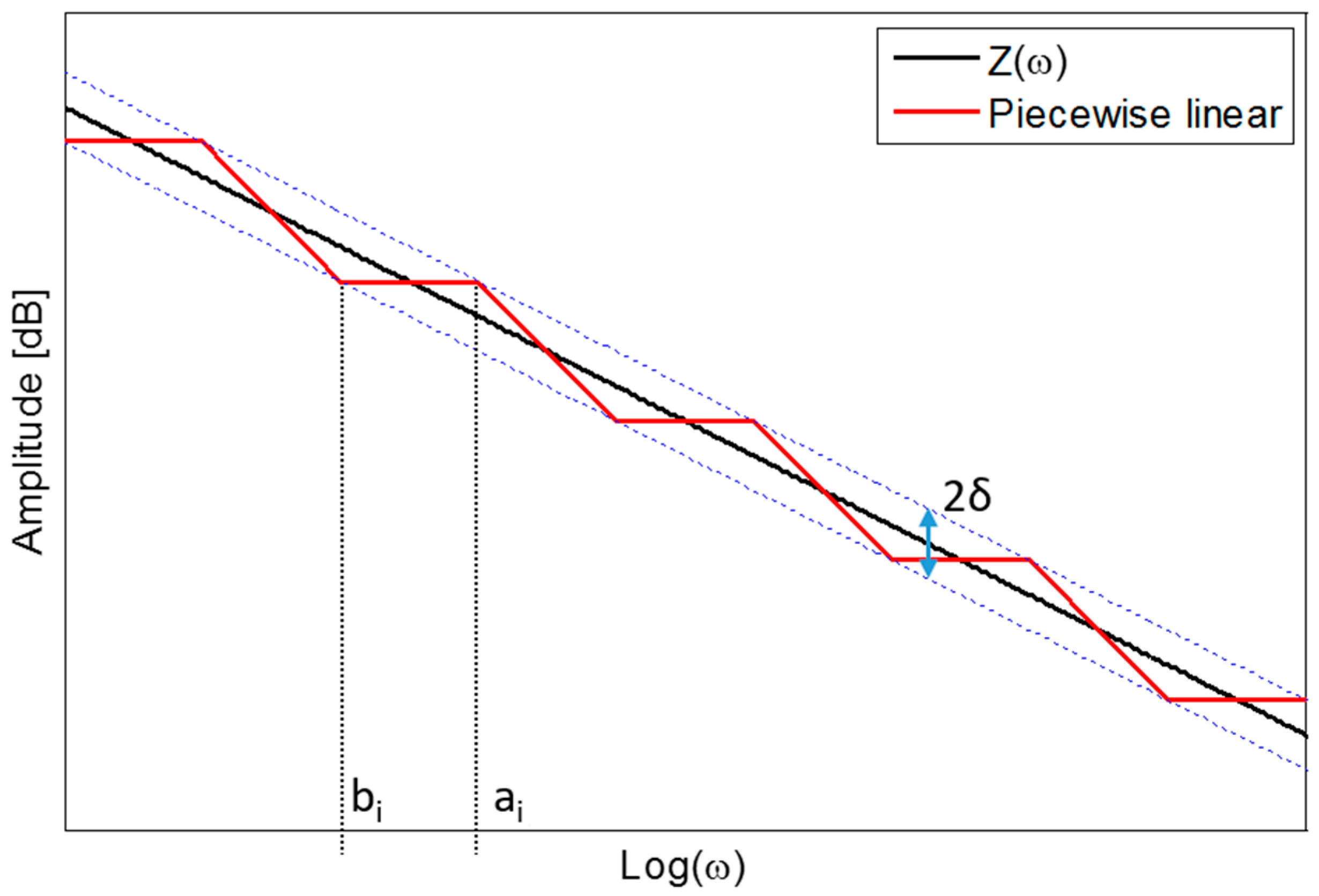
where A, ai, and bi are all positive numbers. Such an expression consists of n first-order damp elements and n first-derivative elements. Each couple of damp and derivative elements, separately considered, represent a piecewise linear function. So, if we consider the operator Z(ω), we can define a tolerance threshold 2δ and require that the piecewise linear is included in the upper and lower boundaries, as shown in Figure 1.
The approximation of the fractional characteristic will be acceptable in a certain bandwidth, depending by the accepted tolerance δ and by the order n of the rational function G(ω). It is worth to define as ω0 the central frequency of the approximation and as Z0 the magnitude of the impedance for ω = ω0. Taking n as odd value and starting from the central point , it is possible to graphically calculate the coefficients ai and bi as:
Once the parameters of (4) have been identified, it is possible to expand the rational approximation as:
where the parameters A0 … An can be calculated as:
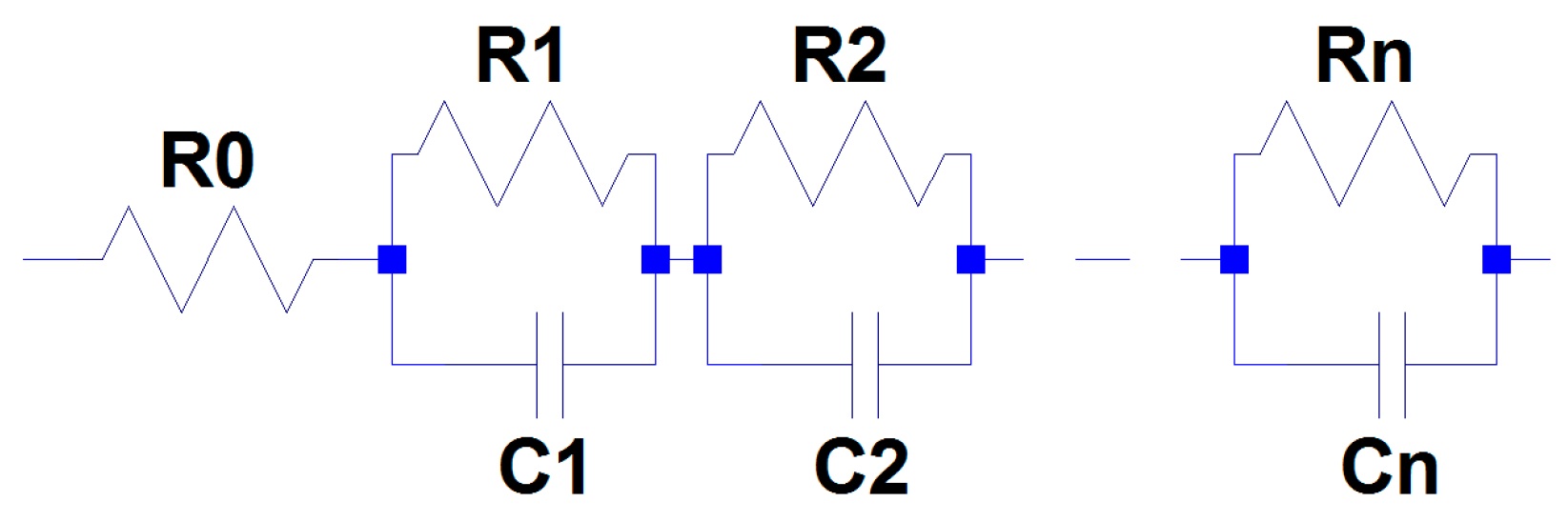
The single first order rational functions composing (9) correspond, in terms of circuits, to a series of R-C parallels where:
In Figure 2, the obtained equivalent circuit is represented, corresponding to a low-pass filter with constant phase.
In order to make a numerical example, let us try to represent a fractance with fractor’s order α = 0.5 and for the representation we choose n = 7, f0 = 100 Hz, Z0 = 50 Ω, and δ = 2 dB. The parameters for the equivalent circuit are obtained as show in Table 1.
3.2. Tuning of the Fractor’s Order
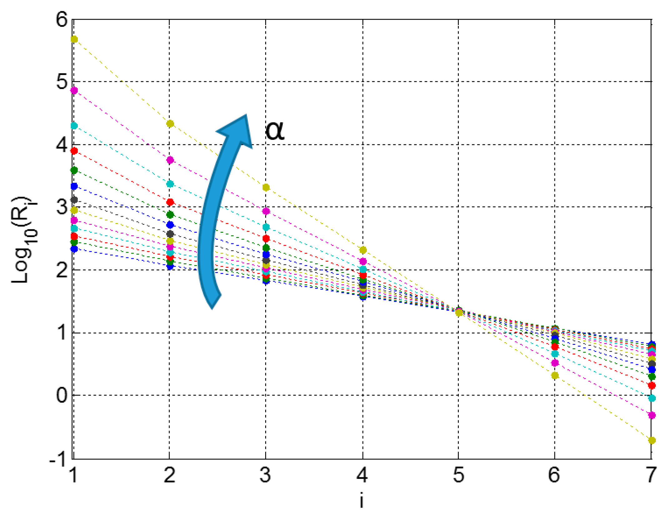
In order to calculate a good approximation of the fractional impedance, every time the fractor’s order α changes, the whole representation should be re-calculated. However, representing the resistances in a logarithmic scale, all the values are on a line that rotates clockwise to the variation of α around the value. For the values of n, ω0, Z0, and δ the variation is show in Figure 5. So, once a set of resistances is found for a given value of α0, is possible to suppose to find a rule for the variation of Ri as function of α.
The family of straight lines can be expressed as:
Once the equivalent network is calculated for a reference fractor’s order α0, it is possible to easily calculate . The, it is found that applying the empirical law:
Additionally, practically it found that the resistances changes with α much more than the capacitances. So, it is worth to consider a network where the resistances vary with α according to (14) and (15) and capacitors are fixed. Such a network is a very good approximation of the fractional impedance for the value of α0 adopted to compute the capacitances. However, it will be able to approximate fractional impedances for different values of α, in a bandwidth always as smaller as the fractor’s order differs from the starting value of α0.
Such a kind of circuit can be easily implemented by means of the same configuration in Figure 2 and adopting traditional capacitors and variable resistors. For instance, by using digital potentiometers connected to a controller, it is possible to program the synchronous variation of all the potentiometers according to the programmed rules, in order to obtain the wished set of resistances and so in the end the wished fractional impedance.
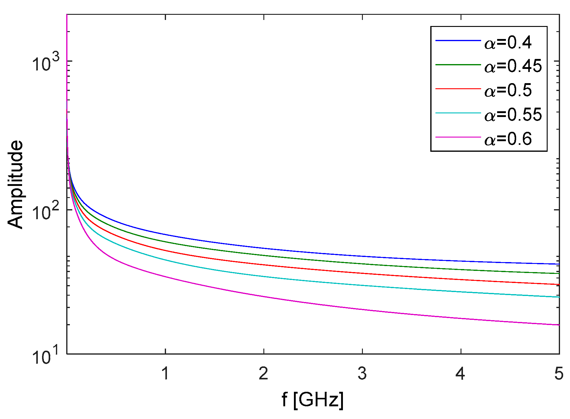
In order to provide a numerical example, we can consider once again the previously values of n, ω0, Z0, and δ. If we consider as reference fractor’s order , then we obtain . This allows to compute the coefficients and then new values of for different values of α.
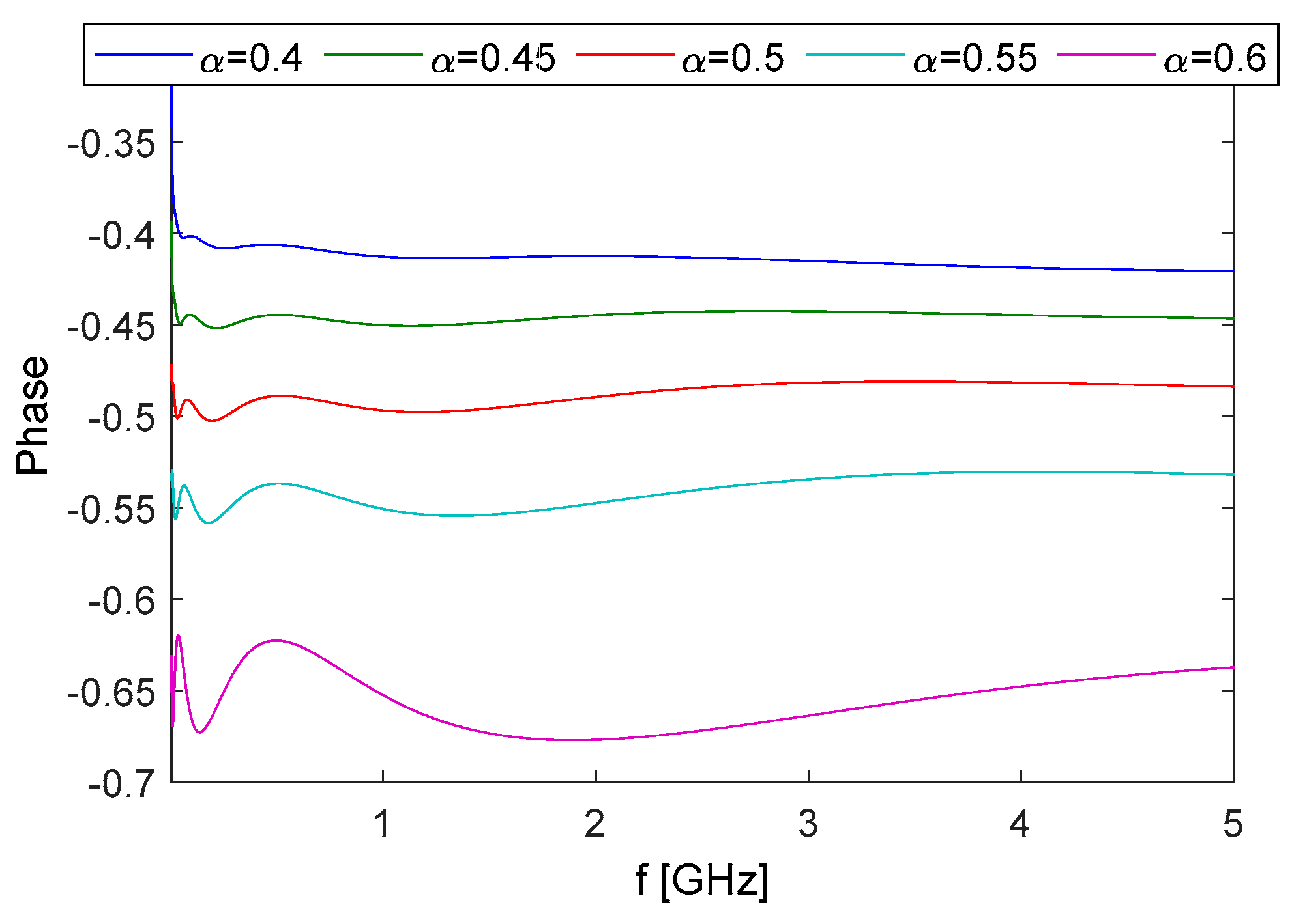
In Figure 6 and Figure 7, we show the amplitude and the phase of the rational approximation G(ω) for different values of α computed with this procedure. The reference amplitudes and phases of Z(ω) are not shown to make the pictures more readable. Anyway, the amplitude comparison would have been neglectable, as for the special case of Figure 3, while the phase of G(ω) has to be compared with a constant value of course.
Again, the amplitude plot represents the fractional impedance in a wider bandwidth than the phase plot.
Moreover, as expected, the quality of the approximation, especially in the phase plot, decreases for higher values of α.
4. Conclusions
In this paper, a methodology for designing a fractional order component with tunable fractor’s order has been proposed. It represents a step forward in the research of equivalent circuits for the practical realization of fractances, since the proposed method allows to realize a unique implementation able to cover a range of fractor’s orders, not requiring any more a new circuit implementation any time the fractor’s order has to be changed. The procedure has been presented in detail and applied to the case of a low-pass microwave filter. Being the procedure generic, it can be easily applied in order to physically implement the circuit on a small board. With a simple control of the digital potentiometers, it is possible to change fractor’s order in a certain range, depending by the number of elements in the ladder and by the accepted tolerance.
A more detailed investigation on the control methodology may allow extending the range of tuning. For this reason, we expect to introduce in the near future an optimization algorithm instead of the empirical procedure in order to improve the method’s performance. In addition, comparison between the designed model and the real implementation will allow to better understand the real effectiveness of the design process.
Funding
This research received no external funding.
Institutional Review Board Statement
Not applicable.
Informed Consent Statement
Not applicable.
Data Availability Statement
Data sharing not applicable.
Conflicts of Interest
The authors declare no conflict of interest.
References
- Caputo, M. Linear model of dissipation whose Q is almost frequency independent—II. Geophys. J. 1967, 13, 529–539. [Google Scholar] [CrossRef]
- Miller, K.S.; Ross, B. An Introduction to the Fractional Calculus and Fractional Differential Equations; John Wiley & Sons, Inc.: New York, NY, USA, 1993. [Google Scholar]
- Oldham, K.B.; Spanier, J. The Fractional Calculus: Theory and Application of Differentiation and Integration to Arbitrary Order; Academic Press: New York, NY, USA, 1974. [Google Scholar]
- Machado, J.A.T.; Kiryakova, V.; Mainardi, F. Kiryakova and F. Mainardi. Recent History of Fractional Calculus. Commun. Nonlinear Sci. Numer. Simul. 2011, 16, 1140–1153. [Google Scholar] [CrossRef] [Green Version]
- Gutiérrez, R.E.; Rosário, J.M.; Machado, J.A.T. Fractional Order Calculus: Basic Concepts and Engineering Applications. Math. Probl. Eng. 2010, 2010, 375858. [Google Scholar] [CrossRef] [Green Version]
- Debnath, L. Recent applications of fractional calculus to science and engineering. Int. J. Math. Math. Sci. 2003, 2003, 3413–3442. [Google Scholar] [CrossRef] [Green Version]
- Dalir, M.; Bashour, M. Applications of Fractional Calculus. Appl. Math. Sci. 2010, 4, 1021–1032. [Google Scholar]
- Dattoli, G.; Ricci, P.; Cesarano, C.; Vazquez, L. Special polynomials and fractional calculus. Math. Comput. Model. 2003, 37, 729–733. [Google Scholar] [CrossRef]
- Assante, D.; Cesarano, C.; Fornaro, C.; Vazquez, L. Higher order and fractional diffusive equations. J. Eng. Sci. Technol. Rev. 2015, 8, 202–204. [Google Scholar] [CrossRef]
- Soltan, A.; Radwan, A.; Soliman, A.M. Fractional order filter with two fractional elements of dependant orders. Microelectron. J. 2012, 43, 818–827. [Google Scholar] [CrossRef]
- Petras, I. Fractional-order nonlinear systems: Modeling, analysis and simulation. Springer Sci. Bus. Media 2011. [Google Scholar]
- Petras, I. Fractional-order memristor-based Chua’s circuit. IEEE Trans. Circuits Syst. II: Express Briefs 2010, 57, 975–979. [Google Scholar] [CrossRef]
- Nakagawa, M.; Sorimachi, K. Basic characteristics of a fractance device. IEICE Trans. Fundam. Electron. Commun. Comput. Sci. 1992, 75, 1814–1819. [Google Scholar]
- Elwakil, A.S. Fractional-order circuits and systems: An emerging interdisciplinary research area. IEEE Circuits Syst. Mag. 2010, 10, 40–50. [Google Scholar] [CrossRef]
- DSierociuk, D.; Podlubny, I.; Petras, I. Experimental evidence of variable-order behavior of ladders and nested ladders. IEEE Trans. Control Syst. Technol. 2013, 21, 459–466. [Google Scholar] [CrossRef]
- Tanwar, R.; Sanjay, K. Analysis & design of fractance based fractional order filter. Int. J. 2013, 1, 113–122. [Google Scholar]
- Upadhyay, D.K.; Mishra, S.K. Realization of fractional order microwave low pass filter. Int. J. Microw. Opt. Technol. 2015, 10, 260–265. [Google Scholar]
- Hamed, E.M.; AbdelAty, A.M.; Said, L.A.; Radwan, A.G. Effect of different approximation techniques on fractional-order KHN filter design. Circuits Syst. Signal Process. 2018, 37, 5222–5252. [Google Scholar] [CrossRef]
- Radwan, A.G.; Elwakil, A.S.; Soliman, A.M. On the generalization of second-order filters to the fractional-order domain. J. Circuits Syst. Comput. 2009, 18, 361–386. [Google Scholar] [CrossRef]
- Abdelouahab, M.S.; Hamri, N. Fractional-order hybrid optical system and its chaos control synchronization. EJTP 2014, 11, 49–62. [Google Scholar]
- Tavazoei, M.S.; Haeri, M. Synchronization of chaotic fractional-order systems via active sliding mode controller. Phys. A Stat. Mech. Its Appl. 2008, 387, 57–70. [Google Scholar] [CrossRef]
- Shahiri, M.; Ghaderi, R.; N., A.R.; Hosseinnia, S.H.; Momani, S. Chaotic fractional-order Coullet system: Synchronization and control approach. Commun. Nonlinear Sci. Numer. Simul. 2010, 15, 665–674. [Google Scholar] [CrossRef]
- Adhikary, A.; Khanra, M.; Pal, J.; Biswas, K. Realization of Fractional Order Elements. INAE Lett. 2017, 2, 41–47. [Google Scholar] [CrossRef] [Green Version]
- Clovis, F.; Daou, A.Z.; Moreau, X. Synthesis and implementation of non integer integrators using RLC. Int. J. Electron. 2009, 12, 1207–1223. [Google Scholar]
- Radwan, A.G.; Salama, K.N. Passive and active elements using fractional circuit. IEEE Trans. Circuits Syst. I Regul. Pap. 2011, 58, 2388–2397. [Google Scholar] [CrossRef]
- Krishna, B.T.; Reddy, K. Active and Passive Realization of Fractance Device of Order ½. Act. Passiv. Electron. Compon. 2008, 2008, 369421. [Google Scholar] [CrossRef] [Green Version]
- Sierociuk, D.; Macias, M.; Malesza, W. Analog Modeling of Fractional Switched Order Derivative Using Different Switching Schemes. IEEE J. Emerg. Sel. Top. Circuits Syst. 2013, 3, 394–403. [Google Scholar] [CrossRef]
- Sugi, M.; Hirano, Y.; Miura, Y.F.; Saito, K. Simulation of fractal immittance by analog circuits: An approach to the optimized circuits. IEICE Trans. Fundam. 1999, 82, 205–209. [Google Scholar]
- Tarunkumar, H.; Ranjan, A.; Kumar, R.; Subrahmanyam, P. Operational Amplifier-Based Fractional Device of Order s±0.5. In Proceeding of International Conference on Intelligent Communication, Control and Devices 2017; Springer: Singapore, 2017; pp. 151–159. [Google Scholar]
- Mondal, D.; Biswas, K. Packaging of single component fractional order element. IEEE Trans. Device Mater. Reliab. 2013, 13, 73–80. [Google Scholar] [CrossRef]
- Elshurafa, A.M.; Almadhoun, M.N.; Salama, K.N.; Alshareef, H.N. Microscale electrostatic fractional capacitors using reduced graphene oxide percolated polymer composites. Appl. Phys. Lett. 2013, 102, 232901. [Google Scholar] [CrossRef]
- Caponetto, R.; Graziani, S.; Pappalardo, F.L.; Sapuppo, F. Experimental characterization of ionic polymer metal composite as a novel fractional order element. Adv. Math. Phys. 2013, 2003, 953695. [Google Scholar] [CrossRef] [Green Version]
- Adhikary, A.; Sen, S.; Biswas, K. Design and hardware realization of a tunable fractional-order series resonator with high quality factor. Circuits Syst. Signal Process. 2017, 36, 3457–3476. [Google Scholar] [CrossRef]
- Wu, M.; Wang, C.; Cai, N.; Meng, W. Fractance circuit design based on a method of constructing the rational approximation function in the form of factorization. In Proceedings of the Control and Decision Conference (IEEE CCDC), Qingdao, China, 23–25 May 2015; pp. 6011–6016. [Google Scholar]
Figure 1.
Example of amplitude behavior of the operator Z(ω) and the piecewise function.

Figure 2.
Equivalent circuit implementing (9).

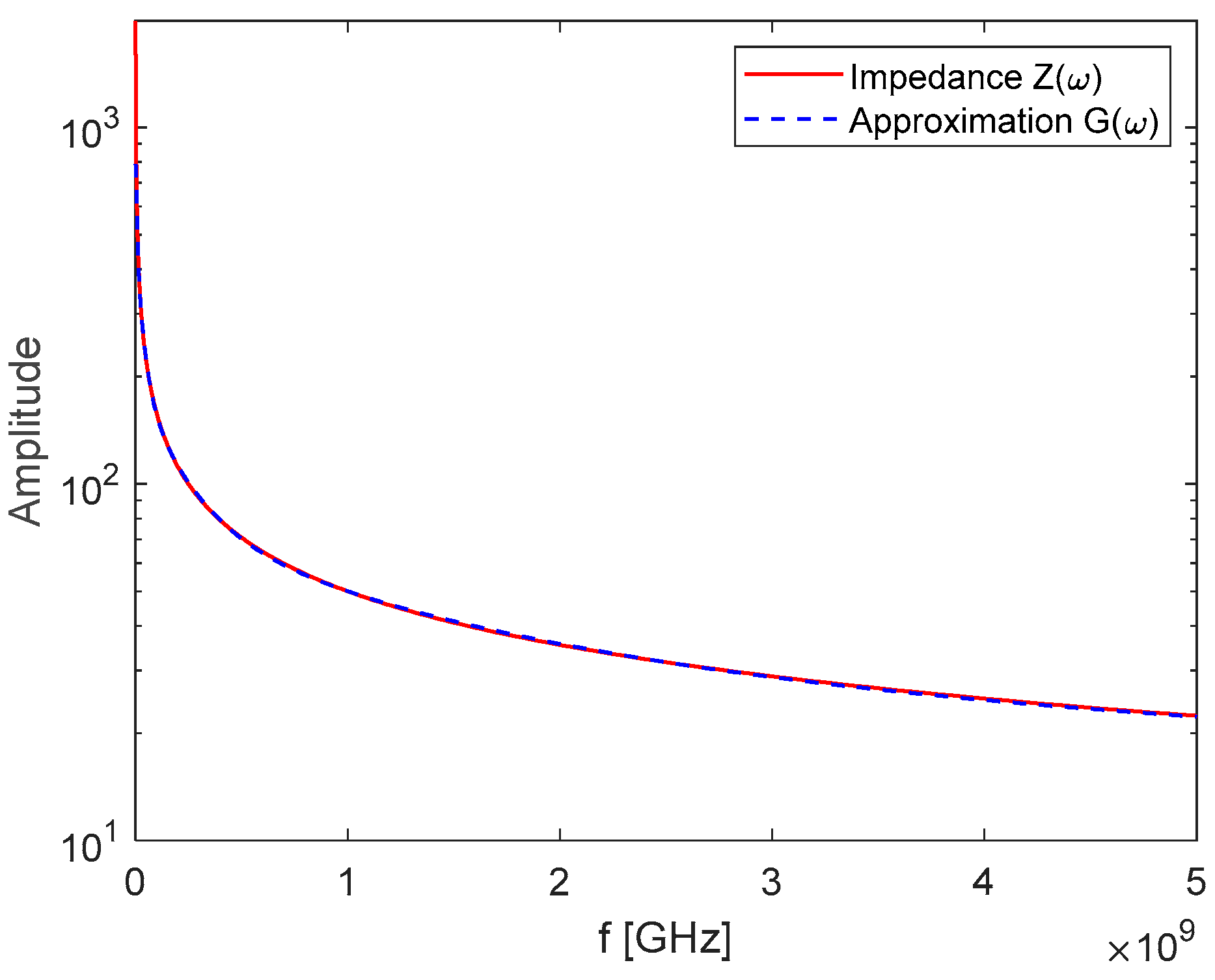
Figure 3.
Amplitude of the impedance Z(ω) and the rational approximation function G(ω).

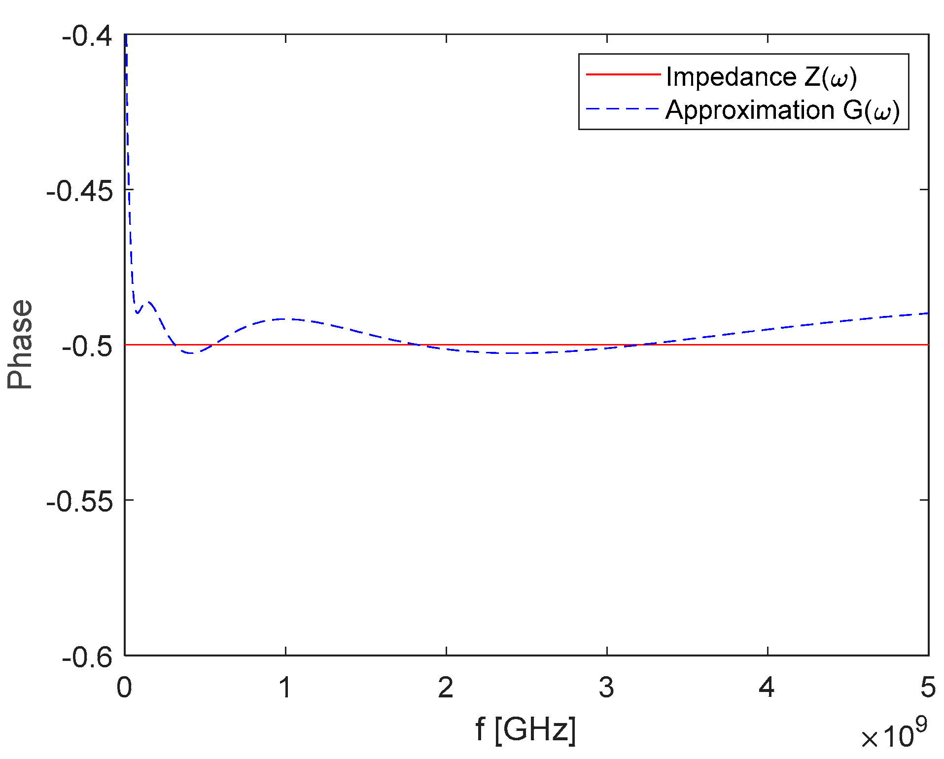
Figure 4.
Phase of the impedance Z(ω) and the rational approximation function G(ω).

Figure 5.
Variation of the resistances Ri as function of α (variable between 0.3 and 0.7).

Figure 6.
Amplitude of the rational approximation G(ω) for different values of α.

Figure 7.
Phase of the rational approximation function G(ω) for different values of α.


Table 1.
Parameters for the equivalent circuit.
| i | 0 | 1 | 2 | 3 | 4 | 5 | 6 |
|---|---|---|---|---|---|---|---|
| R [Ω] | 3.15 | 541 | 154 | 58.9 | 23.2 | 9.10 | 3.26 |
| C [pF] | - | 0.293 | 0.163 | 0.068 | 0.027 | 0.011 | 0.005 |
Publisher’s Note: MDPI stays neutral with regard to jurisdictional claims in published maps and institutional affiliations. |
© 2022 by the author. Licensee MDPI, Basel, Switzerland. This article is an open access article distributed under the terms and conditions of the Creative Commons Attribution (CC BY) license (https://creativecommons.org/licenses/by/4.0/).
Share and Cite
MDPI and ACS Style
Assante, D. Fractance with Tunable Fractor’s Order for Microwave Circuit Applications. Appl. Sci. 2022, 12, 10108. https://0-doi-org.brum.beds.ac.uk/10.3390/app121910108
AMA Style
Assante D. Fractance with Tunable Fractor’s Order for Microwave Circuit Applications. Applied Sciences. 2022; 12(19):10108. https://0-doi-org.brum.beds.ac.uk/10.3390/app121910108
Chicago/Turabian StyleAssante, Dario. 2022. "Fractance with Tunable Fractor’s Order for Microwave Circuit Applications" Applied Sciences 12, no. 19: 10108. https://0-doi-org.brum.beds.ac.uk/10.3390/app121910108
Note that from the first issue of 2016, this journal uses article numbers instead of page numbers. See further details here.