Article

SEM-RCNN: A Squeeze-and-Excitation-Based Mask Region Convolutional Neural Network for Multi-Class Environmental Microorganism Detection

1
Microscopic Image and Medical Image Analysis Group, College of Medicine and Biological Information Engineering, Northeastern University, Shenyang 110819, China
2
School of Intelligent Medicine, Chengdu University of Traditional Chinese Medicine, Chengdu 610075, China
3
International Joint Institute of Robotics and Intelligent Systems, Chengdu University of Information Technology, Chengdu 610225, China
4
School of Resources and Civil Engineering, Northeastern University, Shenyang 110819, China
5
School of Computer Science and Engineering, Northeastern University, Shenyang 110169, China
6
Institute of Medical Informatics, University of Luebeck, 23562 Luebeck, Germany
*
Authors to whom correspondence should be addressed.
Submission received: 7 May 2022 / Revised: 21 September 2022 / Accepted: 25 September 2022 / Published: 1 October 2022
(This article belongs to the Special Issue Low Carbon Water Treatment and Energy Recovery)

Abstract

:
This paper proposes a novel Squeeze-and-excitation-based Mask Region Convolutional Neural Network (SEM-RCNN) for Environmental Microorganisms (EM) detection tasks. Mask RCNN, one of the most applied object detection models, uses ResNet for feature extraction. However, ResNet cannot combine the features of different image channels. To further optimize the feature extraction ability of the network, SEM-RCNN is proposed to combine the different features extracted by SENet and ResNet. The addition of SENet can allocate weight information when extracting features and increase the proportion of useful information. SEM-RCNN achieves a mean average precision (mAP) of 0.511 on EMDS-6. We further apply SEM-RCNN for blood-cell detection tasks on an open source database (more than 17,000 microscopic images of blood cells) to verify the robustness and transferability of the proposed model. By comparing with other detectors based on deep learning, we demonstrate the superiority of SEM-RCNN in EM detection tasks. All experimental results show that the proposed SEM-RCNN exhibits excellent performances in EM detection.

1. Introduction

Environmental Microorganisms (EMs) collectively refer to all microorganisms that have an impact on the environment, including microorganisms living in the natural environment (such as oceans and deserts) and artificial environments (such as fisheries and wheat fields) [1]. There are about 10 11 10 12 types of EMs on Earth [2]. All of them play a positive or negative role in the task of environmental governance. For example, plant rhizosphere-promoting bacteria can help promote plants’ healthy growth. It can also inhibit pathogenic microorganisms that harm plants. However, harmful rhizosphere bacteria can inhibit the normal growth of plants by producing phytotoxins [3]; the emergence of cyanobacteria will accelerate the process of eutrophication of water bodies and damage water quality, which will eventually lead to the death of a large number of aquatic organisms; aspidisca has a strong sensitivity to the chemical substances contained in the water body. Therefore, aspidisca is widely applied for evaluating the quality of the aquaculture water body in the water aquaculture industry. To better play the role of EMs in environmental governance, research on EM detection is essential. The methods of EM detection can be mainly grouped into manual microscope observation methods and computer-aided detection methods.
Manual microscope observation methods refer to the observation and record of EMs in the field of view by an experimenter with certain professional knowledge using a microscope. However, there exist some limitations and disadvantages with respect to manual microscope observation methods. First, the experimenter cannot make quick judgments and must consult many reference materials when facing a wide variety of EMs. Second, all experimenters have to spend a substantial amount of time when learning the basics of EMs and the operation of the microscope. Finally, the detection results obtained by different operators might be different, and the objectivity of the detection results is insufficient [4]. Therefore, manual microscope observation methods have great limitations for EM detection tasks.
Compared to manual microscope observation methods, computer-aided detection methods are more objective, accurate, and convenient. With rapid developments in computer vision and deep learning technologies, computer-assisted image analysis is broadly applied in many research fields, including fire emergency [5], histopathological image analysis [6,7,8,9], cytopathological image analysis [10,11,12], object detection [13,14,15,16,17], microorganism classification [18,19,20,21,22,23], microorganism segmentation [24,25,26,27], and microorganism counting [28,29]. In addition, with the advancement of computer hardware and the rapid development of computer-aided detection methods, the results obtained by computer-aided detection methods in EM detection are improving. Currently, the most popular computer-aided detection method is the EM detection method based on deep learning [30]. However, there is no relevant research on the detection of multi-class EMs. Therefore, we choose some classical detectors based on deep learning for multi-class EM detection and propose a novel detector called squeeze-and-excitation-based mask region convolutional neural network (SEM-RCNN). The flowchart of SEM-RCNN is shown in Figure 1.
In Figure 1, three main parts are contained. Part one is the original dataset part, which includes enough images of EMs for model training and testing. We will introduce the specific information about the original dataset in detail in the experimental section. Part two is the data-processing part. In this part, the original dataset is firstly labeled in the format of the object detection dataset. Then, all data are grouped into the training set, validation set, and test set according to a certain proportion. Part three is the EM detection part. Firstly, the original SEM-RCNN is pre-trained on Microsoft Common Objects in Context (MS-COCO) dataset. Then the proposed model is finetuned and trained on the training and validation sets of EMDS-6. After that, the detection performance of the trained model is verified on the test set. Finally, we evaluate the detection results of SEM-RCNN by employing appropriate evaluation indicators.
The main contributions of this paper are listed as follows:
  • A novel detector based on convolutional neural network (CNN): SEM-RCNN is proposed for multi-class EM detection;
  • The block of SENet is designed to combine with ResNet as the backbone of the proposed SEM-RCNN, which can extract features with a self-attention mechanism;
  • The proposed SEM-RCNN achieves the optimal detection performance both for small (EMDS-6) and large (blood cell) datasets.
To illustrate the proposed method clearer, the structure of this paper is designed as follows: In Section 2, the related research about computer-aided EM detection is summarized; In Section 3, detailed information about SEM-RCNN is introduced; In Section 4, the detailed operation of the experiments is introduced, including experimental data, experimental settings, evaluation criteria, detection results, and extensive experiment; In Section 5, the paper is summarized comprehensively.

2. Related Work

In this section, we group all computer-aided EM detection methods into classical image-processing-based methods, traditional machine-learning-based methods, and deep-learning-based methods. The detection methods are introduced based on relevant research studies.

2.1. Classical Image Processing Based Methods

Classical image-processing-based methods are the earliest computer-aided methods for EM detection. Classical image-processing-based methods contain two subcategories of detection methods, segmentation-based methods, and classification-based methods.
Thresholding-based methods are the most used technologies for image segmentation, such as in [31,32,33,34,35,36,37,38,39,40,41,42,43,44,45,46,47,48]. Thresholding methods are the most commonly used methods in image segmentation. In addition, thresholding methods can select an appropriate threshold for detection according to different EMs, which gives these methods strong generalization abilities. In [32], an area threshold was applied for Chlamydomonas and Chlamydomonas bicuspidata detection. In [37], the multiple thresholds method was employed for motile microorganisms. Multiple thresholds were firstly applied to binarize input images. Then, all white regions are regarded as EMs. In [40], the color threshold was applied for tubercle bacillus detection. In [43], adaptive threshold and global threshold were applied for nematode detection. An adaptive threshold was employed for binarizing the original image. Then, a global threshold was applied for extracting reference labels. By combining these two processed images, the nematode can be detected. Among all these works, the Otsu threshold is the most used one. In [33,42,44,45,46], the Otsu threshold is applied for different EMsdetection. The main idea of Otsu was to select an optimal threshold automatically from a gray-level histogram by a discriminant criterion [49]. The Otsu threshold can provide good results with simple calculations. Even if the gray value of the object to be segmented is similar to the gray value of the background, the Otsu threshold can achieve good segmentation results. However, due to the limitation of the calculation method, when the difference between the foreground and the background area is too large, the Otsu threshold cannot achieve a good segmentation result [50].
Classification-based methods apply shape features, geometric features, color features, texture features, and statistical features for EM detection, such as in [51,52,53,54,55,56,57,58,59,60,61,62,63,64,65]. In [51,52,55], shape features were selected as vital information for EM detection, including contour features, area features, squareness, angular, roundness, etc. In [56], a contour feature was used for detecting Methanospirillum hungatei and Methanosarcina mazei. In [52], a C. elegans nematode worm detection method based on angular features was designed. In [55], roundness was selected as the criterion for judging whether the detected objects are Rotavirus-A particles. In [57,59,60,61,62,63,66], geometric features were selected for EM detection. In [60], the area was regarded as an important indicator for judging the presence of bacteriophage. In [61], the most suitable combination of some kinds of geometric features was selected and applied for bacilli detection. In [62,63], an automatic detection method based on area-to-length ratio was proposed for six different airborne fungi spores. In [57,61], color features were employed for initial screening regions containing EMs. In [64], a Anabaena and Oscillatoria detection method based on texture features was proposed. From all these classification based methods, we can find that shape features are the most suitable feature for EM detection. In addition, detection methods by combining different features can achieve improved detection performances than a single feature.

2.2. Traditional Machine-Learning-Based Methods

Since 2006, traditional machine-learning-based methods have been gradually applied in the field of EM detection, such as in [67,68,69,70,71,72,73,74,75,76,77,78,79]. The main idea of this method is to determine the EMs category according to the acquired feature information and the corresponding network structure. In [67], a back propagation neural network was employed for bacteria detection. After several preprocessing steps such as threshold-based segmentation and denoising, morphological features of bacteria are extracted and then sent to a back propagation neural network for detection. In [68], a genetic algorithm-neural network method was presented for tubercle bacillus detection. By applying a color filter, moving k-means clustering, and region growing, a suitable segmented image was obtained, which is then sent to the color filter, moving k-means clustering and region growing for the final detection. In [69], a probabilistic neural network is applied for pathogens detection. First, the original image is processed by background correction and object isolation. Then, regions that may contain pathogens were selected. At last, a probabilistic neural network is built for pathogen detection.
Based on the research on traditional machine learning methods in this field, we find that the most widely used classification model is the support vector machine (SVM) classifier, mentioned in [70,71,72,73,74,75,76,77,78,79]. SVM can construct an optimal separation hyperplane in the feature space of the data to maximize the gap between positive and negative samples in the training set [80], which makes SVM an efficient classifier for binary classification tasks. Furthermore, SVM can efficiently use smaller training samples. This enables SVM in achieving higher classification accuracies on a smaller training set. Therefore, after the development of related technologies of SVM, it has been gradually applied to the detection of EMs. In [71], an SVM classifier is proposed for P. minimum species detection. In addition, to improve the accuracy of the detection results, the SVM classifier is combined with a random forest classifier. In [74], a multi-class SVM was proposed for EM detection. First, the Sobel edge detector is applied for image segmentation. After that, shape features, Fourier descriptors, and some other features were extracted from processed images and then sent to a multi-class SVM for detecting EMs. In [78], an SVM classifier is applied for planktonic organisms detection. The preprocessing step includes threshold segmentation, robust refocusing criterion, and re-segmentation. After that, the processed image is detected by an SVM classifier.

2.3. Deep-Learning-Based Methods

Compared with methods based on traditional machine learning, deep-learning-based methods have the advantages of the wide range of applications and high applicability. In the feature extraction step of detection processing, traditional machine-learning-based methods use manual feature engineering methods, which are labor-intensive and time-consuming. Deep-learning-based methods can achieve automatic feature learning through advanced network structures and complex features compared to simple ones. Therefore, with the development of deep learning technologies, increasing research about EM detection using deep learning methods is presented, such as in [81,82,83,84,85,86,87,88,89,90]. In [81,82,83], CNN was employed for EM detection. In [81], a tubercle bacillus detector was designed based on CNN. In [83], a CNN-based method was proposed for actinobacterial species detection. In [88], a region convolutional neural network (R-CNN)-based detector was proposed for diatom detection. In addition, a you only look once (YOLO)-based detector is prepared for comparisons. The result indicates that YOLO performs better than R-CNN in diatom detection. In [84,85,86,87], Faster R-CNN-based methods were employed for EM detection. In [85], a Faster R-CNN-based detector was proposed for parasite egg detection. In [87], Faster R-CNN was applied for algal detection. About 1859 samples were prepared for the test.
After consulting all these related research studies, we found that classical image-processing-based methods were mainly used as preprocessing methods in current EM detection studies. The most widely used methods in EM detection are traditional machine-learning-based methods. Although there are a few studies about deep-learning-based methods, deep-learning-based methods show great potential in EM detection. Therefore, we designed a deep-learning-based detector for EM detection called SEM-RCNN.

3. SEM-RCNN-Based EM Detection Method

The structure of the proposed SEM-RCNN is shown in Figure 2, which mainly includes the input step, feature extraction step, region proposal step, a mapping step between candidate boxes and feature maps, and the output step.
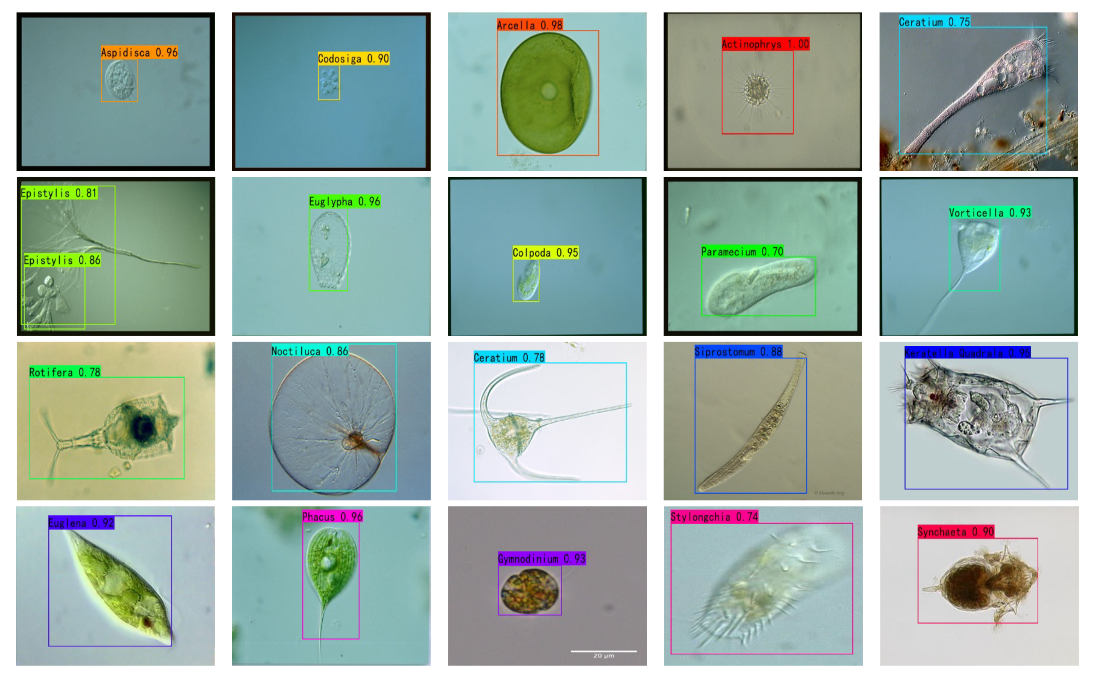
Figure 2: (a) Input: The dataset contains images of 21 types of EMs and their corresponding labeled images. There are 840 images in total, and each type has 40 original images (Section 4.1 and Section 4.2.1 for details). (b) Feature extraction: A combination network based on SENet and feature pyramid network (FPN) is proposed for fuller and deeper feature extraction (Section 3.1 for details). (c) Region proposal: A region proposal network (RPN) was applied to obtain multi-candidate boxes of the object (Section 3.2 for details). (d) Mapping between candidate boxes and feature maps: The method based on the region of interesting align (ROI align) is applied for accurate mapping between candidate boxes and the feature map, as well as the mapping between the feature map and the fixed size feature map (Section 3.3 for details). (e) Output: A multi-branched structure is applied for feature maps regression, and the combined approach of the fully connected layer, bounding box regression, and Softmax is applied for object detection (Section 3.4 for details).

3.1. Feature Extraction Step

The feature extraction step is the basis for deep learning to perform all tasks. Therefore, whether a suitable feature extraction network is selected or not directly affects final detection results. After analyzing and comparing the existing networks, we finally chose the deep residual network (ResNet) [91] combined with a squeeze-and-excitation network (SENet) [92] as the basic backbone, together with the feature pyramid network(FPN) [93]. ResNet can solve the degradation problem occurring in the training process of CNN. SENet can effectively enhance the needed feature information while suppressing less useful feature information. FPN can achieve the accurate detection of multi-scale objects by making good use of shallow feature information and deep feature information.

3.1.1. ResNet

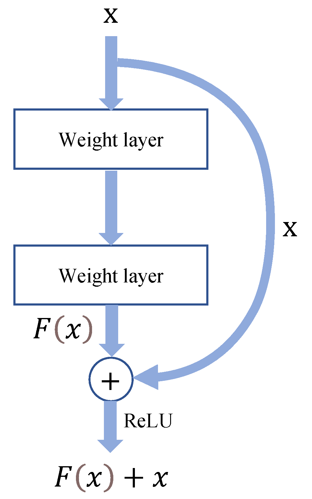
The main contribution of ResNet concerns an inevitable problem in the training of CNN, called the degradation problem. In general, as the number of layers of the network model increases, the overall detection effectiveness of the CNN model improves. However, when the number of layers deepens to a certain level, the effectiveness of the CNN model decreases, which is the degradation problem that occurs when CNN is trained. The idea of residual learning is introduced with conventional CNNs in ResNet to solve the degradation problem encountered in the deep training of CNN. The structure of a residual block is shown in Figure 3, where x denotes features learned by the shallow network; F(x) is the residual function. The residual block allows the deep network to learn new features relative to the shallow network continuously. From Figure 3, the actual features learned by the network after the residual block are F(x) + x, which means that a deep network can obtain deeper and more complex features from the features extracted by the shallow network based on the introduction of the residual block.

3.1.2. SENet

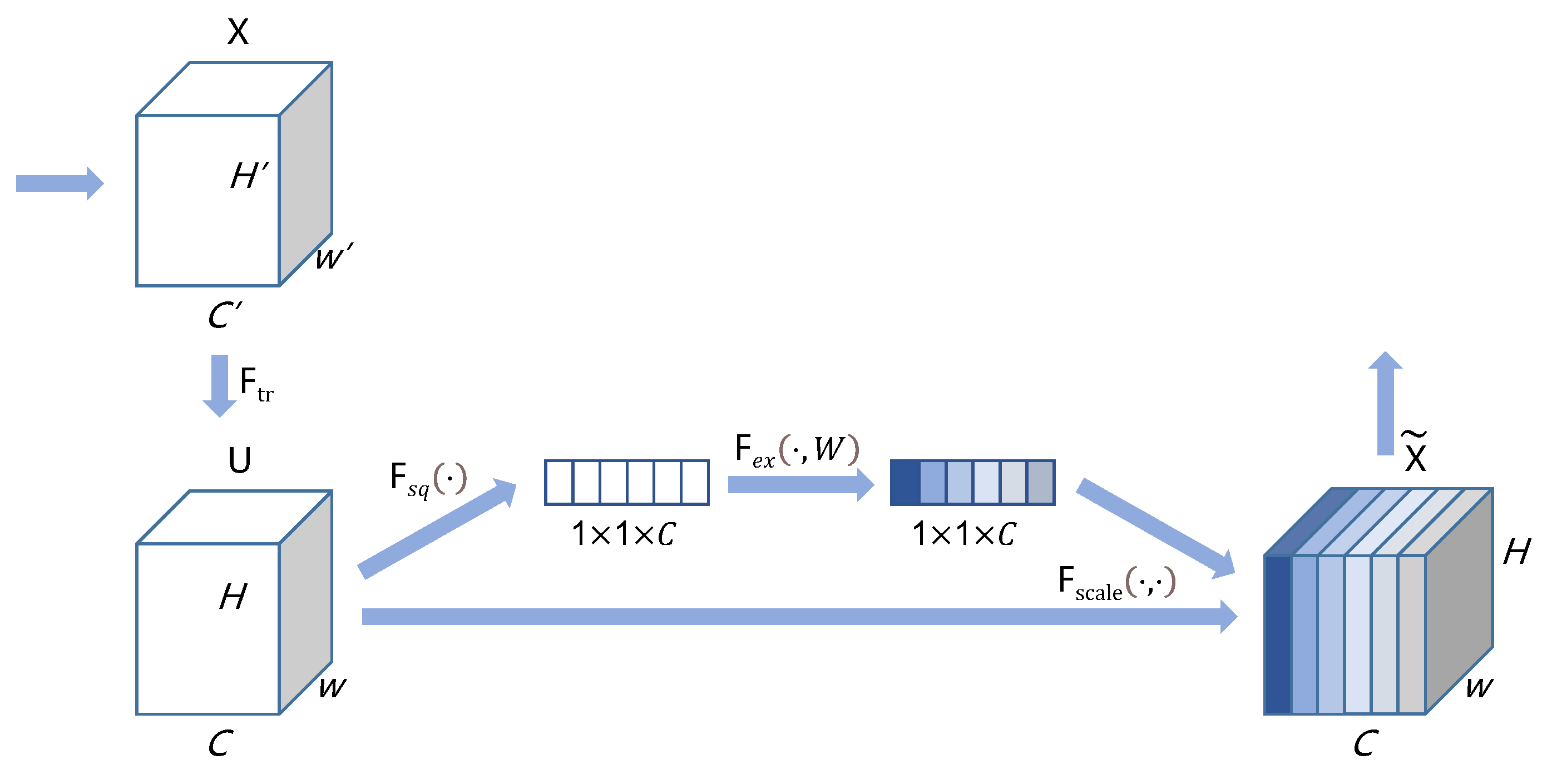
SENet is a network structure that focuses on enhancing data channel information and enhancing desired feature information while suppressing less useful feature information based on the self-attention mechanism. SE block is the basic module of SENet and can be well integrated with many existing models. The corresponding experimental classification and detection results show that the combination with an SE block can increase the feature representation capability of the model and, thus, improve the classification or detection effects of the model. The basic structure of the SE block is shown in Figure 4. Among them, F t r is the traditional convolution operation. X and U represent the input and output of this convolution operation, respectively; C, W, H, C′, W′, and H′ represent the scales of data; function F s q and F e x represent the two core processes of the SE block, squeeze processing and excitation processing; X ˜ represents the final output of the SE block.
In the SE process, a squeeze operation is first performed on the convolution output. To make better use of the interconnected information between input data channels, the SE block first uses the idea of averaging to convert the information of all pixels involved in a plane into a specific value. The specific calculation procedure for averaging is shown in Equation (1).
z c = F s q ( u c ) = 1 H × W i = 1 H j = 1 W u c ( i , j )
In Equation (1), z c represents the squeeze output of the c channel data of input data; u c represents the c channel data of input data. It can be seen from the formula that input data eventually become a column vector in the squeeze process. The length of this vector is the same as the number of channels, and each data value in this vector is closely related to the corresponding channel data.
After that, to further exploit the interlinked information between channels, SE designs an excitation process. The equation for this process is shown in Equation (2).
s = F e x ( z , W ) = σ ( g ( z , W ) ) = σ ( W 2 σ ( W 1 z ) )
In Equation (2), σ is the rectified linear unit (ReLU) activation function; W 1 R C r × C ; W 2 R C × C r ; W 1 is the dimensionality reduction layer with a dimensionality reduction ratio of r. W 2 is the proportionally identical data-dimensionality increase layer. After the excitation process, the complexity of the entire model is controlled. Moreover, vital features are enhanced, and weak features are limited based on the self-attention mechanism. Moreover, the generalization ability of the model is enhanced. The sigmoid function processes the final output of the excitation process to a value between zero and one.
The final output of the SE block multiplies the value obtained after compression and activation processing with the data of all the channels that U has. Based on such processing, the SE block can enhance features that have a greater impact on the experimental results while weakening features that have a smaller impact on experimental results.

3.1.3. FPN

FPN is a network component that assists CNN in detecting objects with different scales. From the comparison of the information contained in shallow and deep features, shallow features have richer location information and are more suitable for predicting the location coordinates of the object; deep features have richer category information and are more suitable for predicting the category of the object. Therefore, a suitable combination of shallow and deep features can achieve the accurate detection of EMs, which is the main idea of FPN. FPN consists of three main network structures: down–up processing, up–down processing, and horizontal linkage of feature layers, as shown in Figure 5.
Down–up processing is the feedforward process of CNN. By non-stop convolutional operations, multiple feature maps of different scales are obtained in this step. After that, the feature maps output by the deepest level network are up-sampled by the operation to keep the same size as the feature maps output by the previous level network. Then, upsampled feature maps are fused with the feature maps outputted by the previous layer network. Feature maps obtained based on FPN are richer in feature information than traditional feature maps. In addition, to better fuse the information of each map, FPN processes the fusion between feature maps by using the horizontal linkage operation. The horizontal linkage is performed by convolutional processing using a 1 × 1 -sized convolutional kernel. In general, FPN can combine the rich location information of shallow feature maps and the rich category information of deep feature maps to provide accurate categories and locations of objects at different scales without increasing computational efforts.

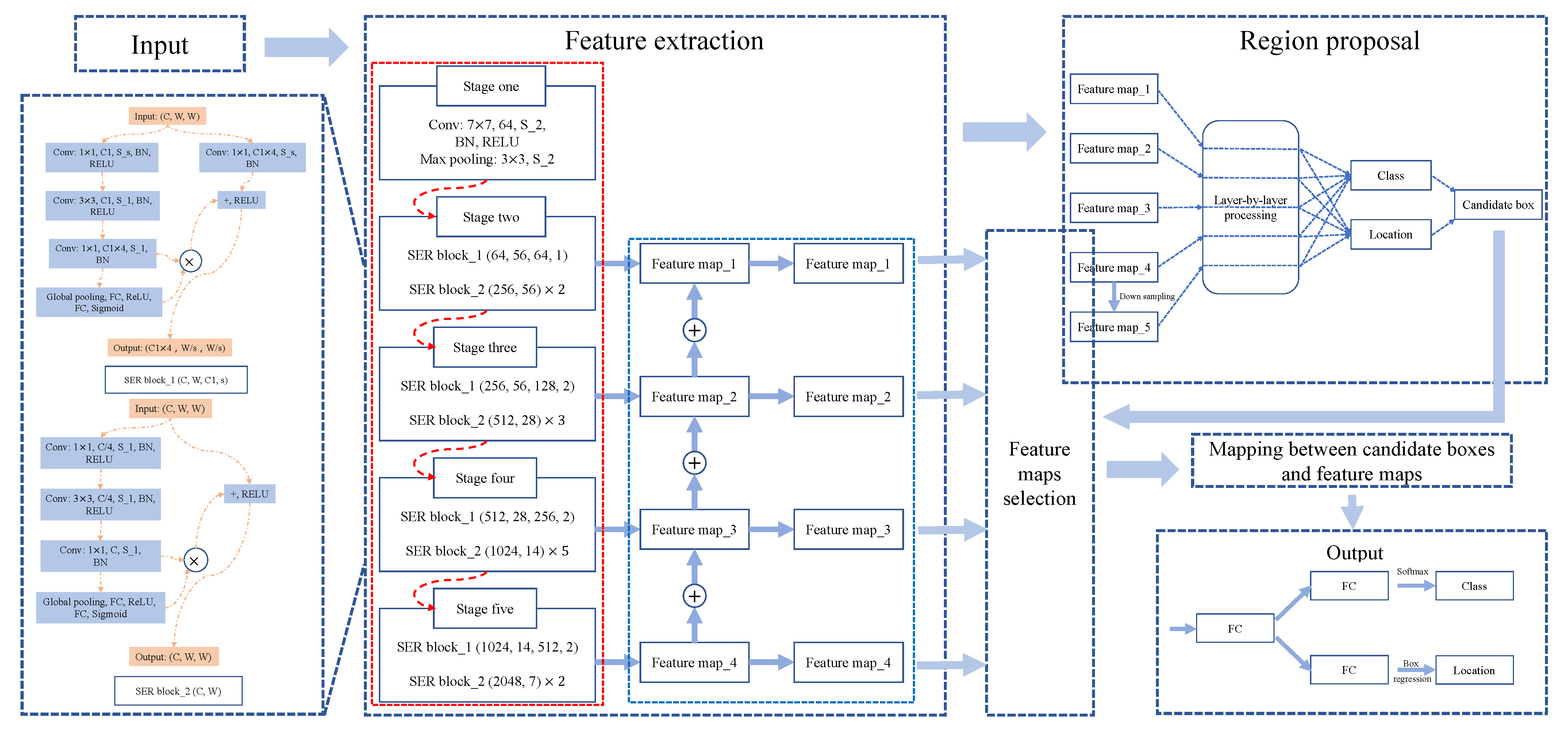
3.1.4. Backbone of Feature Extraction Step

By fusing ResNet, SENet, and FPN, we finally design the backbone of SEM-RCNN, as shown in Figure 6. There are mainly five steps in the red dashed box in Figure 6. In stage one, 64 convolution kernels with a kernel size of 7 × 7 and a stride of 2, followed by batch normalization (BN) and ReLU operations, were applied for feature extraction. Then, max-pooling with a size of 3 × 3 and stride of 2 was applied to reduce the size of feature maps. After that, the following four steps are based on the combination approach of SER block_1 and SER block_2. The SER block_1 and SER block_2 are important parts of the backbone, and its structure are shown in Figure 7. From Figure 7, we can see that the SER block_1 is mainly used to deal with the case where the input and output dimensions are different; the SER block_2 is mainly used to deal with the case where input and output dimensions are the same. For the input parameters of SER block_1, the channel of the input image is denoted as C, the width (same as height) of the input image is denoted as W, the output channel of the feature map is denoted as C1, and the stride is denoted as s. For example, in stage two of Figure 6, input images are processed at the size of 54 × 54 with 64 channels. Hence, in the first step of SER block_1, 64 convolution kernels with the kernel size of 1 × 1 and stride of 1 (followed by BN and ReLU operations) were applied first. Then, the convolution kernels with the kernel size of 3 × 3 and 1 × 1 were applied sequentially to extract the feature and to adjust channels. At the same time, the input image is processed by 64 × 4 convolution kernels with the kernel size of 1 × 1 and stride of 1 (right part of SER block_1). Finally, the feature maps after global pooling and sigmoid (the left part of SER block_1) are residually connected with the right part of SER block_1. The output size of SER block_1 is 56 × 56 with channels of 64 × 4. The structure of SER block_2 is similar to SER block_1, but the output size is the same as the input size. The combination method of SER block_1 and SER block_2 repeats four times in SEM-RCNN for feature extraction.
Based on our sufficient research foundation [15,20,21,22,24,29], it can be found that only a few studies employed deep learning methods to perform the detection task in microorganism image analysis. Since the detection task in microorganism image analysis has strong application background, almost all studies directly utilize existing deep learning models, such as RCNN [88] and Faster R-CNN [84,85]. Different from these studies, we proposed a novel self-attention-based two-stage detection framework, which is inspired by ResNet, SENet, and FPN. This framework achieves state-of-the-art performances on the detection task, which significantly promotes the development of the detection technology in the application of microorganism image analyses.

3.2. Region Proposal Step

Generating candidate boxes for objects is an important processing step of an object detector. In this step, a suitable target candidate frame needs to be generated based on the input feature map. Here, we choose the region proposal network (RPN) to accomplish the task of candidate boxes proposal for SEM-RCNN. RPN can generate prediction boxes for objects with different scales in a short period. RPN mainly includes three processing steps: generating anchor boxes, judging the category of generated anchor boxes, and adjusting the position of anchor boxes. The main flow of RPN is shown in Figure 8. First, RPN generates a certain amount of anchor boxes based on the input feature map; after that, the generated Anchor boxes are convolved with a convolution kernel of 3 × 3 ; then, the Softmax function and the border regression algorithm are used to distinguish prospect and background of boxes and obtain position coordinates of the predicted boxes respectively; finally, the candidate boxes are determined based on the obtained category scores and position coordinates.

3.3. RoI Align

After obtaining suitable boxes, the detector needs to associate the obtained boxes with feature maps. Here, RoI Align is employed to this end. The main idea of RoI Align is to use bilinear interpolation to obtain the value of floating-point coordinates. Therefore, RoI Align chooses to keep the floating-point coordinates in determining the corresponding area in the feature map based on the position coordinates of the candidate box. When dividing the area corresponding to the candidate box on the feature map equally into multiple small fixed-size feature maps, RoI Align chooses to maintain the segmented boundaries instead of performing quantization operations. Eventually, bilinear interpolation allows the RoI Align to obtain the feature values corresponding to the four coordinate positions of each small feature map.
Bilinear interpolation is the calculation of the value of a pixel point (floating point) that does not exist in the location image from the value of a known pixel point. The bilinear interpolation method can be computed by performing two horizontal interpolation operations and then one vertical interpolation or by performing two vertical interpolation operations and then one horizontal interpolation. Here, the specific calculation process of the bilinear interpolation method with lateral interpolation followed by vertical interpolation is introduced. The specific coordinates of Q 11 , Q 21 , Q 12 , Q 22 , R 1 , R 2 and P involved in the formula are shown in Figure 9.
First is the first horizontal interpolation calculation, as shown in Equation (3).
f ( R 1 ) x 2 x x 2 x 1 f ( Q 11 ) + x x 1 x 2 x 1 f ( Q 21 )
This is followed by a second horizontal interpolation calculation, as shown in Equation (4).
f ( R 2 ) x 2 x x 2 x 1 f ( Q 12 ) + x x 1 x 2 x 1 f ( Q 22 )
The last step is calculation of the value of P point based on the two transverse interpolation results (f( R 1 ) and f( R 2 )) obtained from above calculation, as shown in Equation (5).
f ( P ) y 2 y y 2 y 1 f ( R 1 ) + y y 1 y 2 y 1 f ( R 2 )

3.4. Output

The final goal of SEM-RCNN is to obtain the bounding box and class of object. Therefore, in the output part of SEM-RCNN, the feature map after RoI Align processing is first classified using a fully connected (FC) layer. Then, the output of the coordinate information of the object is realized by the FC layer and border regression; the output of the class information of the object is realized by the fully connected layer and Softmax function. Finally, the task of target detection is accomplished by combining border coordinate information and class information, as shown in Figure 10.

4. Experiment Results and Analysis

4.1. Dataset

We use the Environmental Microorganism Dataset Sixth Version (EMDS-6) [94]. The original EMs images with their corresponding ground truth (GT) images of 21 types of EMDS-6 are shown in Figure 11.
EMDS-6 includes 21 types of EMs that have 840 original images and 840 ground truth images, respectively, as shown in Figure 11. There are 21 categories with 40 images in each category. In the training process, the dataset is evenly distributed to each category for balanced training. In our work, we perform object annotation using Lambelme software based on original and ground truth images provided by EMDS-6. Most of the images in EMDS-6 only contain one type of EM.

4.2. Experimental Settings

4.2.1. Data Settings

For EMDS-6, each type of EM is randomly grouped into training, validation, and test dataset with a ratio of 4:1, which means 32 images are applied for training (with 5-fold cross validation), and the last 8 images are applied for testing. Though the dataset is small for training a complex model, it can still achieve excellent detection performance by using transfer learning [94].

4.2.2. Hyper-Parameter Settings

In the process of training, the proposed SEM-RCNN model is pre-trained on the MS-COCO dataset, firstly. Then, the training step of SEM-RCNN contains two steps. The head is frozen and trained with an epoch of 150 and a learning rate of 0.0001. After that, the whole network is trained with an epoch of 150 and a learning rate of 0.001. The final model parameters have the lowest loss function obtained on the validation set. There are 98,793,356 trainable parameters of SEM-RCNN in total. The intersection over union (IoU) is the ratio of intersection and concatenation of the prediction box and true box. A result can be considered a correct detection only if the IoU value of the prediction box is greater than the set threshold, so the IoU threshold is a critical hyperparameter that may highly affect the performance of the proposed model. To systematically choose the IoU threshold, we test the detection performance of different IoU settings using SEM-RCNN based on SE-ResNet-101. The IoU threshold is set from 0.1 to 0.9 with the stride of 0.1, and the average detection indices based on 5-fold cross validation are shown in Table 1.
By reviewing Table 1, we find that the set of IoU thresholds is critical for the detection performance of the proposed model. The highest mAP, Precision, Recall, and F1-score can be obtained when the IoU threshold is set as 0.3. Though the mean IoU is higher when the threshold is set as 0.4, 0.8, and 0.9, the other indices (such as Precision) are not satisfactory. Therefore, by considering the aggregate detection performance, the IoU threshold is set as 0.3, which performs accurately and balanced.

4.3. Evaluation Criteria

We use mean average precision (mAP) as the evaluation metric in our experiments. mAP, as the best evaluation metric for the target detection task, combines the accuracy of detection category and location. The calculation of mAP is shown in Equation (6).
m A P = 1 n i = 1 n A P i
In Equation (6), n presents the number of classes of EMs; AP is determined by the area under the accuracy-precision curve. The calculations of accuracy and precision are related to true positive (TP), true negative (TN), false positive (FP), false negative (FN), and intersection over union (IoU). The description of TP, TN, FP, and FN is shown in Table 2. The calculations of accuracy and precision are shown in Equations (7) and (8), respectively.
Accuracy = TP + TN TP + TN + FP + FN
Precision = TP TP + FP

4.4. Detection Results and Analysis

The detection results of SEM-RCNN on EMDS-6 is shown in Figure 12.
The loss curves while training and validation are shown in Figure 13. It shows that the bounding box loss and classification loss curves of the proposed SEM-RCNN can converge steadily and quickly, which indicates that the proposed SEM-RCNN model has satisfactory performance on bounding box regression and object classification tasks.
In order to show more intuitively how the SEM-RCNN compares with other detectors, we compare them in the form of a table in the following. In Table 3, we compared the average detection indices (with 5-fold cross validation) of SEM-RCNN and Mask RCNN on EMDS-6 when combined with ResNet-50 and ResNet-101.
From Table 3, we can find that SEM-RCNN proposed in this paper can achieve better detection performance than Mask RCNN both in single-object and multi-object for EM detection. Overall, the models based on the backbone of ResNet-101 and SE-ResNet-101 perform better than those based on ResNet-50 and SE-ResNet. Compared with the original ResNet-based Mask RCNN, the performance increment of SEM-RCNN based on deeper SE-ResNet is much better than the Mask RCNN based on deeper ResNet both for mAP, precision, recall, and F1-score. Moreover, the mAP of the proposed SEM-RCNN achieves 0.511, which is much better than the result of Mask RCNN. The confusion matrix of the proposed SEM-RCNN is shown in Figure 14, showing the classification performance of the proposed model.
From Figure 14, most of the test images can be classified correctly. However, there still exists some mis-detected images. For example, 5 images of Codosiga are wrongly classified as Epistylis, showing the large error rate of the proposed model. By referring to the images of the two EMs in Figure 15, we find that the EMs have similar morphological features, and both are clustered microorganisms.
Moreover, by reviewing Figure 14, we find that Stentor is easily classified as Paramecium, an example is shown in Figure 16. Most EMs are colorless and transparent, so the morphological feature determines the classification result. However, though the EMs are in variance shapes, they may perform similar shapes at different growth phases. On the other hand, the quantity and quality of the dataset will have a greater impact on the model’s performance. However, the satisfactory EM dataset is relatively difficult to obtain due to some objective reasons, such as the impurities in the acquisition environment, uneven natural light, and other adverse factors. So the model still cannot classify similar EMs accurately due to the small dataset.

4.5. Extensive Experiment

To compare the detection performance of SEM-RCNN with existing deep learning-based detectors, we chose several classical detectors for our experiments. Table 4 introduces the detection results and population variances (with 5-fold cross validation) of some classical deep-learning-based detectors.
From the final detection results, SEM-RCNN achieves better detection performance than SSD, Faster R-CNN, RetinaNet, YOLOv3, and YOLOv4. The results prove that it is feasible to improve the detection effectiveness of a detector by increasing its feature extraction capability.
To further prove the object detection performance of the proposed SEM-RCNN model, another dataset of EMs should be applied for the extensive experiment. However, by reviewing our previous works about EMs image analysis and EMs dataset [15,18,19,20,21,22,24,25,26,28,29,95], there are few proper open-access EMs dataset, which is caused by several objective reasons, including the uneven natural lighting and too many impurities while imaging. Hence, a dataset containing 8 types of blood cells is applied for the extensive experiment, including erythrocytes, basophils, eosinophils, lymphocytes, monocytes, neutrophils, platelets, and immunoglobulins. The reasons why we choose the blood cell images consisting four aspects: firstly, the images of EMs and blood cells are both microscopic images, which have strong morphological and shape similarities; secondly, both of them are non-directional images, where all objects in these images have no fixed positive direction; thirdly, both of them can be applied for multi-class detection tasks; finally, both of them have lots of noise and redundant impurities. Besides, the application of the blood cell image dataset can prove the strong generalization ability of the proposed SEM-RCNN. There are 17,090 labeled blood cell images in total, and the proposed SEM-RCNN is trained for 150 epochs with finetuning based on the pre-trained model for MS-COCO dataset. The result is shown in Table 5. By reviewing Table 5, we find that the proposed SEM-RCNN can achieve excellent blood cell detection performance. Most of the evaluation metrics are more than 0.9, which performs better than Mask RCNN significantly. The detection result is shown in Figure 17, which shows satisfactory detection performance of the proposed SEM-RCNN.

5. Conclusions and Future Work

The analysis and research of EMs are essential. Therefore, a suitable method for EM detection needs to be explored. After summarizing and analyzing the work related to EM detection, we designed the SEM-RCNN for the detection of EMs. In terms of applications, to fully demonstrate the feasibility of SEM-RCNN for EM detection, model training and testing were conducted in a small dataset of EMs and a large dataset of blood cells, respectively. The final detection results demonstrate the feasibility of SEM-RCNN for detecting EMs. In terms of technology, an improved method combining Mask RCNN with SENet is proposed in this paper. To verify the feasibility of the improved method, the detection results of SEM-RCNN and the original Mask RCNN are compared on the EMDS-6 dataset and blood cell dataset, respectively. The comparison results showed that the detection results of SEM-RCNN improved two to three points in mAP than that of the original Mask RCNN. Finally, SEM-RCNN achieved a 0.511 mAP on EMDS-6 and 0.907 mAP on the blood cell dataset.
This paper fills the gap in computer-aided multi-class EM detection research. However, considering the continuous innovation of related technologies and the challenges that need to be faced in practical applications, there is still more research potential and room for improvement in several aspects of this study. Regarding current research results, further research content with respect to our work will mainly be considered from EMs data. From the detection results on dataset EMDS-6 and blood cell dataset, it can be seen that sufficient training data can significantly improve the detection effect of the model. In contrast, insufficient training data can lead to poor detection effects from the model. Therefore, in the follow-up study, we will focus part of our efforts on expanding the existing microbial dataset to build an EMs dataset with more sufficient data and to better meet the training of detection models.

Author Contributions

J.Z. (Jiawei Zhang), Methodology, validation, data curation, writing—original draft preparation, review and editing, and visualization; P.M., methodology, software, validation, formal analysis, data curation, writing—original draft preparation, and visualization; T.J., investigation; funding acquisition; X.Z., resources; W.T., resources; J.Z. (Jinghua Zhang), validation; S.Z., validation; X.H., validation; M.G., investigation; C.L., conceptualization, methodology, data curation, writing—original draft preparation, writing—review and editing, supervision, and project administration. All authors have read and agreed to the published version of the manuscript.

Funding

This work is supported by the “Natural Science Foundation of China” (No. 61806047 and 61971118) and “Sichuan Science and Technology Program” (No. 2021YFH0069, 2021YFQ0057, and 1614 2022YFS0565).

Data Availability Statement

EMDS-6 is at: https://figshare.com/articles/dataset/EMDS-6/17125025/1 (accessed on 15 February 2022).

Acknowledgments

We thank Zixian Li and Guoxian Li for their important discussions. We also thank M.E. Pingli Ma, due to his contribution is considered as important as the first author in this paper.

Conflicts of Interest

There is no conflict of interest in this paper.

Abbreviations

The following abbreviations are used in this manuscript:
EMsenvironmental microorganisms;
CNNconvolutional neural network;
MS-COCOmicrosoft common objects in context;
SEM-RCNNsqueeze-and-excitation-based mask region convolutional neural network;
RCNNregion convolutional neural network;
FCfully connected;
ReLUrectified linear unit;
BNbatch normalization;
SVMsupport vector machine;
YOLOyou only look once;
ResNetdeep residual network;
SENetsqueeze-and-excitation network;
FPNfeature pyramid network;
RPNregion proposal network;
EMDS-6the Environmental Microorganism Dataset Sixth Version;
mAP             mean average precision;
TPtrue positive;
TNtrue negative;
FPfalse positive;
FNfalse negative;
IoUintersection over union;
GTground truth.

References

  1. Pepper, I.L.; Gerba, C.P.; Gentry, T.J.; Maier, R.M. Environmental Microbiology; Academic Press: Cambridge, MA, USA, 2011. [Google Scholar]
  2. Locey, K.J.; Lennon, J.T. Scaling laws predict global microbial diversity. Proc. Natl. Acad. Sci. USA 2016, 113, 5970–5975. [Google Scholar] [CrossRef] [PubMed] [Green Version]
  3. Nehl, D.B.; Allen, S.J.; Brown, J.F. Deleterious rhizosphere bacteria: An integrating perspective. Appl. Soil Ecol. 1997, 5, 1–20. [Google Scholar] [CrossRef]
  4. Van Deun, A.; Salim, A.H.; Cooreman, E.; Hossain, M.A.; Rema, A.; Chambugonj, N.; Hye, M.; Kawria, A.; Declercq, E. Optimal tuberculosis case detection by direct sputum smear microscopy: How much better is more? Int. J. Tuberc. Lung Dis. 2002, 6, 222–230. [Google Scholar] [PubMed]
  5. Sharma, J.; Granmo, O.C.; Goodwin, M. Emergency Analysis: Multitask Learning with Deep Convolutional Neural Networks for Fire Emergency Scene Parsing. In Proceedings of the International Conference on Industrial, Engineering and Other Applications of Applied Intelligent Systems, Kuala Lumpur, Malaysia, 26–29 July 2021; Springer: Cham, Switzerland, 2021; pp. 101–112. [Google Scholar]
  6. Li, X.; Li, C.; Rahaman, M.M.; Sun, H.; Li, X.; Wu, J.; Yao, Y.; Grzegorzek, M. A comprehensive review of computer-aided whole-slide image analysis: From datasets to feature extraction, segmentation, classification and detection approaches. Artif. Intell. Rev. 2022, 55, 4809–4878. [Google Scholar] [CrossRef]
  7. Li, Y.; Li, C.; Li, X.; Wang, K.; Rahaman, M.M.; Sun, C.; Chen, H.; Wu, X.; Zhang, H.; Wang, Q. A Comprehensive Review of Markov Random Field and Conditional Random Field Approaches in Pathology Image Analysis. Arch. Comput. Methods Eng. 2021, 29, 609–639. [Google Scholar] [CrossRef]
  8. Zhou, X.; Li, C.; Rahaman, M.M.; Yao, Y.; Ai, S.; Sun, C.; Wang, Q.; Zhang, Y.; Li, M.; Li, X.; et al. A comprehensive review for breast histopathology image analysis using classical and deep neural networks. IEEE Access 2020, 8, 90931–90956. [Google Scholar] [CrossRef]
  9. Li, C.; Chen, H.; Li, X.; Xu, N.; Hu, Z.; Xue, D.; Qi, S.; Ma, H.; Zhang, L.; Sun, H. A review for cervical histopathology image analysis using machine vision approaches. Artif. Intell. Rev. 2020, 53, 4821–4862. [Google Scholar] [CrossRef]
  10. Liu, W.; Li, C.; Rahaman, M.M.; Jiang, T.; Sun, H.; Wu, X.; Hu, W.; Chen, H.; Sun, C.; Yao, Y.; et al. Is the aspect ratio of cells important in deep learning? A robust comparison of deep learning methods for multi-scale cytopathology cell image classification: From convolutional neural networks to visual transformers. Comput. Biol. Med. 2022, 141, 105026. [Google Scholar] [CrossRef]
  11. Rahaman, M.M.; Li, C.; Yao, Y.; Kulwa, F.; Wu, X.; Li, X.; Wang, Q. DeepCervix: A deep learning-based framework for the classification of cervical cells using hybrid deep feature fusion techniques. Comput. Biol. Med. 2021, 136, 104649. [Google Scholar] [CrossRef]
  12. Rahaman, M.M.; Li, C.; Wu, X.; Yao, Y.; Hu, Z.; Jiang, T.; Li, X.; Qi, S. A survey for cervical cytopathology image analysis using deep learning. IEEE Access 2020, 8, 61687–61710. [Google Scholar] [CrossRef]
  13. Zou, S.; Li, C.; Sun, H.; Xu, P.; Zhang, J.; Ma, P.; Yao, Y.; Huang, X.; Grzegorzek, M. TOD-CNN: An effective convolutional neural network for tiny object detection in sperm videos. Comput. Biol. Med. 2022, 146, 105543. [Google Scholar] [CrossRef] [PubMed]
  14. Chen, A.; Li, C.; Zou, S.; Rahaman, M.M.; Yao, Y.; Chen, H.; Yang, H.; Zhao, P.; Hu, W.; Liu, W.; et al. SVIA dataset: A new dataset of microscopic videos and images for computer-aided sperm analysis. Biocybern. Biomed. Eng. 2022, 42, 204–214. [Google Scholar] [CrossRef]
  15. Ma, P.; Li, C.; Rahaman, M.M.; Yao, Y.; Zhang, J.; Zou, S.; Zhao, X.; Grzegorzek, M. A state-of-the-art survey of object detection techniques in microorganism image analysis: From classical methods to deep learning approaches. Artif. Intell. Rev. 2022, 1–72. [Google Scholar] [CrossRef] [PubMed]
  16. Jung, H.K.; Choi, G.S. Improved YOLOv5: Efficient Object Detection Using Drone Images under Various Conditions. Appl. Sci. 2022, 12, 7255. [Google Scholar] [CrossRef]
  17. Li, X.; Wang, C.; Ju, H.; Li, Z. Surface Defect Detection Model for Aero-Engine Components Based on Improved YOLOv5. Appl. Sci. 2022, 12, 7235. [Google Scholar] [CrossRef]
  18. Zhao, P.; Li, C.; Rahaman, M.; Xu, H.; Yang, H.; Sun, H.; Jiang, T.; Grzegorzek, M. A Comparative Study of Deep Learning Classification Methods on a Small Environmental Microorganism Image Dataset (EMDS-6): From Convolutional Neural Networks to Visual Transformers. Front. Microbiol. 2022, 13, 792166. [Google Scholar] [CrossRef]
  19. Kulwa, F.; Li, C.; Zhang, J.; Shirahama, K.; Kosov, S.; Zhao, X.; Jiang, T.; Grzegorzek, M. A new pairwise deep learning feature for environmental microorganism image analysis. Environ. Sci. Pollut. Res. 2022, 29, 51909–51926. [Google Scholar] [CrossRef]
  20. Kosov, S.; Shirahama, K.; Li, C.; Grzegorzek, M. Environmental microorganism classification using conditional random fields and deep convolutional neural networks. Pattern Recognit. 2018, 77, 248–261. [Google Scholar] [CrossRef]
  21. Li, C.; Shirahama, K.; Grzegorzek, M. Environmental microbiology aided by content-based image analysis. Pattern Anal. Appl. 2016, 19, 531–547. [Google Scholar] [CrossRef]
  22. Li, C.; Shirahama, K.; Grzegorzek, M. Application of content-based image analysis to environmental microorganism classification. Biocybern. Biomed. Eng. 2015, 35, 10–21. [Google Scholar] [CrossRef]
  23. Rahaman, M.M.; Li, C.; Yao, Y.; Kulwa, F.; Rahman, M.A.; Wang, Q.; Qi, S.; Kong, F.; Zhu, X.; Zhao, X. Identification of COVID-19 samples from chest X-Ray images using deep learning: A comparison of transfer learning approaches. J. X-ray Sci. Technol. 2020, 28, 821–839. [Google Scholar] [CrossRef] [PubMed]
  24. Zhang, J.; Li, C.; Yin, Y.; Zhang, J.; Grzegorzek, M. Applications of artificial neural networks in microorganism image analysis: A comprehensive review from conventional multilayer perceptron to popular convolutional neural network and potential visual transformer. Artif. Intell. Rev. 2022, 1–58. [Google Scholar] [CrossRef] [PubMed]
  25. Kulwa, F.; Li, C.; Zhao, X.; Cai, B.; Xu, N.; Qi, S.; Chen, S.; Teng, Y. A state-of-the-art survey for microorganism image segmentation methods and future potential. IEEE Access 2019, 7, 100243–100269. [Google Scholar] [CrossRef]
  26. Zhao, P.; Li, C.; Rahaman, M.M.; Xu, H.; Ma, P.; Yang, H.; Sun, H.; Jiang, T.; Xu, N.; Grzegorzek, M. EMDS-6: Environmental Microorganism Image Dataset Sixth Version for Image Denoising, Segmentation, Feature Extraction, Classification, and Detection Method Evaluation. Front. Microbiol. 2022, 1334. [Google Scholar] [CrossRef] [PubMed]
  27. Li, C.; Zhang, J.; Kulwa, F.; Qi, S.; Qi, Z. A SARS-CoV-2 Microscopic Image Dataset with Ground Truth Images and Visual Features. In Proceedings of the Chinese Conference on Pattern Recognition and Computer Vision (PRCV), Nanjing, China, 16–18 October 2020; Springer: Cham, Switzerland, 2020; pp. 244–255. [Google Scholar]
  28. Zhang, J.; Xu, N.; Li, C.; Rahaman, M.M.; Yao, Y.D.; Lin, Y.H.; Zhang, J.; Jiang, T.; Qin, W.; Grzegorzek, M. An application of Pixel Interval Down-sampling (PID) for dense tiny microorganism counting on environmental microorganism images. arXiv 2022, arXiv:2204.0134112, 7314. [Google Scholar] [CrossRef]
  29. Zhang, J.; Li, C.; Rahaman, M.M.; Yao, Y.; Ma, P.; Zhang, J.; Zhao, X.; Jiang, T.; Grzegorzek, M. A Comprehensive Review of Image Analysis Methods for Microorganism Counting: From Classical Image Processing to Deep Learning Approaches. Artif. Intell. Rev. 2022, 55, 2875–2944. [Google Scholar] [CrossRef]
  30. Prada, P.; Brunel, B.; Reffuveille, F.; Gangloff, S.C. Technique Evolutions for Microorganism Detection in Complex Samples: A Review. Appl. Sci. 2022, 12, 5892. [Google Scholar] [CrossRef]
  31. Bloem, J.; Veninga, M.; Shepherd, J. Fully automatic determination of soil bacterium numbers, cell volumes, and frequencies of dividing cells by confocal laser scanning microscopy and image analysis. Appl. Environ. Microbiol. 1995, 61, 926–936. [Google Scholar] [CrossRef] [Green Version]
  32. Qing, S.; Wu, Y.; Juan, J.; Zhao, X.; Que, X. Application of Microscopic Color Image Processing in Algae Recognition and Statistics. Agric. Mech. Res. 2006, 6, 199–203. [Google Scholar]
  33. Zhang, C.; Chen, W.; Liu, W.; Chen, C. An automated bacterial colony counting system. In Proceedings of the 2008 IEEE International Conference on Sensor Networks, Ubiquitous, and Trustworthy Computing (SUTC 2008), Taichung, Taiwan, 11–13 June 2008; pp. 233–240. [Google Scholar]
  34. Rizvandi, N.B.; Pizurica, A.; Philips, W.; Ochoa, D. Edge linking based method to detect and separate individual C. Elegans worms in culture. In Proceedings of the 2008 Digital Image Computing: Techniques and Applications, Canberra, ACT, Australia, 1–3 December 2008; pp. 65–70. [Google Scholar]
  35. Rizvandi, N.B.; Pizurica, A.; Rooms, F.; Philips, W. Skeleton analysis of population images for detection of isolated and overlapped nematode C. elegans. In Proceedings of the 2008 16th European Signal Processing Conference, Lausanne, Switzerland, 25–29 August 2008; pp. 1–5. [Google Scholar]
  36. Zhou, B.T.; Baek, J.H. Using Machine Vision to Detect Distinctive Behavioral Phenotypes of Thread-shape Microscopic Organism. In Applications of Computational Intelligence in Biology; Springer: Berlin/Heidelberg, Germany, 2008; pp. 161–182. [Google Scholar]
  37. Wang, P.; Wen, C.; Li, W.; Chen, Y. Motile microorganism tracking system using micro-visual servo control. In Proceedings of the 2008 3rd IEEE International Conference on Nano/Micro Engineered and Molecular Systems, Sanya, China, 6–9 January 2008; pp. 178–182. [Google Scholar]
  38. Fernandez, H.; Hintea, S.; Csipkes, G.; Pellow, A.; Smith, H. Machine vision application to the detection of micro-organism in drinking water. In Proceedings of the International Conference on Knowledge-Based and Intelligent Information and Engineering Systems, Zagreb, Croatia, 3–5 September 2008; Springer: Cham, Switzerland, 2008; pp. 302–309. [Google Scholar]
  39. Zhai, Y.; Liu, Y.; Zhou, D.; Liu, S. Automatic identification of mycobacterium tuberculosis from ZN-stained sputum smear: Algorithm and system design. In Proceedings of the 2010 IEEE International Conference on Robotics and Biomimetics, Tianjin, China, 14–18 December 2010; pp. 41–46. [Google Scholar]
  40. Raof, R.A.A.; Mashor, M.Y.; Ahmad, R.B.; Noor, S.S.M. Image segmentation of Ziehl-Neelsen sputum slide images for tubercle bacilli detection. Image Segm. 2011, 2011, 365–378. [Google Scholar]
  41. Shi, H.; Shi, Y.; Yin, Y. Food bacteria auto identification method based on image treatment. J. Jilin Univ. (Eng. Technol. Ed.) 2012, 42, 1049–1053. [Google Scholar]
  42. Badsha, S.; Mokhtar, N.; Arof, H.; Lim, Y.A.L.; Mubin, M.; Ibrahim, Z. Automatic Cryptosporidium and Giardia viability detection in treated water. EURASIP J. Image Video Process. 2013, 2013, 56. [Google Scholar] [CrossRef] [Green Version]
  43. Kowalski, M.; Kaczmarek, P.; Kabaciński, R.; Matuszczak, M.; Tranbowicz, K.; Sobkowiak, R. A simultaneous localization and tracking method for a worm tracking system. Int. J. Appl. Math. Comput. Sci. 2014, 24, 599–609. [Google Scholar] [CrossRef] [Green Version]
  44. Rachna, H.B.; Swamy, M.S.M. Detection of Tuberculosis bacilli using image processing techniques. Int. J. Soft Comput. Eng. 2013, 3, 47–51. [Google Scholar]
  45. Kurtulmuş, F.; Ulu, T.C. Detection of dead entomopathogenic nematodes in microscope images using computer vision. Biosyst. Eng. 2014, 118, 29–38. [Google Scholar] [CrossRef]
  46. Goyal, A.; Roy, M.; Gupta, P.; Dutta, M.K.; Singh, S.; Garg, V. Automatic detection of mycobacterium tuberculosis in stained sputum and urine smear images. Arch. Clin. Microbiol. 2015, 6, 1. [Google Scholar]
  47. Javidi, B.; Moon, I.; Yeom, S.; Carapezza, E. Three-dimensional imaging and recognition of microorganism using single-exposure on-line (SEOL) digital holography. Opt. Express 2005, 13, 4492–4506. [Google Scholar] [CrossRef]
  48. Fernandez-Canque, H.; Beggs, B.; Smith, E.; Boutaleb, T.; Smith, H.; Hintea, S. Micro-organisms detection in drinking water using image processing. Cell 2006, 15, 4-2. [Google Scholar]
  49. Otsu, N. A threshold selection method from gray-level histograms. IEEE Trans. Syst. Man Cybern. 1979, 9, 62–66. [Google Scholar] [CrossRef] [Green Version]
  50. Lee, H.; Park, R. Comments on" An optimal multiple threshold scheme for image segmentation. IEEE Trans. Syst. Man Cybern. 1990, 20, 741–742. [Google Scholar] [CrossRef]
  51. Javidi, B.; Yeom, S.; Moon, I.; Daneshpanah, M. Real-time automated 3D sensing, detection, and recognition of dynamic biological micro-organic events. Opt. Express 2006, 14, 3806–3829. [Google Scholar] [CrossRef] [PubMed]
  52. Huang, K.M.; Cosman, P.; Schafer, W.R. Automated detection and analysis of foraging behavior in Caenorhabditis elegans. J. Neurosci. Methods 2008, 171, 153–164. [Google Scholar] [CrossRef] [PubMed] [Green Version]
  53. Moon, I.; Yi, F.; Javidi, B. Automated three-dimensional microbial sensing and recognition using digital holography and statistical sampling. Sensors 2010, 10, 8437–8451. [Google Scholar] [CrossRef] [PubMed]
  54. Javidi, B.; Moon, I.; Daneshpanah, M. Detection, identification and tracking of biological micro/nano organisms by computational 3D optical imaging. In Proceedings of the Biosensing III. International Society for Optics and Photonics, Nanjing, China, 13 July 2010; Volume 7759, p. 77590R. [Google Scholar] [CrossRef]
  55. Hiremath, P.S.; Bannigidad, P.; Hiremath, M. Segmentation and identification of rotavirus—A in digital microscopic images using active contour model. In Thinkquest∼2010; Springer: Berlin/Heidelberg, Germany, 2011; pp. 177–181. [Google Scholar]
  56. Dubuisson, M.; Jain, A.K.; Jain, M.K. Segmentation and classification of bacterial culture images. J. Microbiol. Methods 1994, 19, 279–295. [Google Scholar] [CrossRef]
  57. Fang, S.P.; Hsu, H.J.; Hung, L.L.; Wu, Y.S. Automatic Identification of Mycobacterium Tuberculosis in Acid-Fast Stain Sputum Smears with Image Processing and Neural Networks; Department of Electronic Engineering: Tainan, Taiwan, 2008. [Google Scholar]
  58. Ogawa, M.; Tani, K.; Ochiai, A.; Yamaguchi, N.; Nasu, M. Multicolour digital image analysis system for identification of bacteria and concurrent assessment of their respiratory activity. J. Appl. Microbiol. 2005, 98, 1101–1106. [Google Scholar] [CrossRef] [PubMed]
  59. Liu, P.Y.; Chin, L.K.; Ser, W.; Ayi, T.C.; Yap, P.H.; Bourouina, T.; Leprince-Wang, Y. Virus infectivity detection by effective refractive index using optofluidic imaging. In Proceedings of the 18th International Conference on Miniaturized Systems for Chemistry and Life Sciences, MicroTAS, San Antonio, TX, USA, 26–30 October 2014. [Google Scholar]
  60. Yu, J.Q.; Huang, W.; Chin, L.K.; Lei, L.; Lin, Z.P.; Ser, W.; Chen, H.; Ayi, T.C.; Yap, P.H.; Chen, C.H.; et al. Droplet optofluidic imaging for λ-bacteriophage detection via co-culture with host cell Escherichia coli. Lab Chip 2014, 14, 3519–3524. [Google Scholar] [CrossRef] [PubMed] [Green Version]
  61. Forero, M.; Cristobal, G.; Alvarez-Borreg, J. Automatic identification techniques of tuberculosis bacteria. In Applications of Digital Image Processing XXVI; International Society for Optics and Photonics: Bellingham, WA, USA, 2003; Volume 5203, pp. 71–81. [Google Scholar]
  62. Perner, P.; Perner, H.; Janichen, S.; Buhring, A. Recognition of airborne fungi spores in digital microscopic images. In Proceedings of the 17th International Conference on Pattern Recognition, ICPR 2004, Cambridge, UK, 26 August 2004; Volume 3, pp. 566–569. [Google Scholar]
  63. Sklarczyk, C.; Perner, H.; Rieder, H.; Arnold, W.; Perner, P. Image acquisition and analysis of hazardous biological material in air. In Proceedings of the International Conference on Mass Data Analysis of Images and Signals in Medicine, Biotechnology, and Chemistry, Leipzig, Germany, 18 July 2007; Springer: Berlin/Heidelberg, Germany, 2007; pp. 1–14. [Google Scholar]
  64. Thiel, S.; Wiltshire, R.J. The automated detection of cyanobacteria using ddigital image processing techniques. Environ. Int. 1995, 21, 233–236. [Google Scholar] [CrossRef]
  65. Jan, Z.; Rafiq, M.; Muhammad, H.; Zada, N. Detection of tuberculosis bacteria in sputum slide image using morphological features. In Proceedings of the International Conference: Beyond Databases, Architectures and Structures, Ustroń, Poland, 26–29 May 2015; Springer: Cham, Switzerland, 2015; pp. 408–414. [Google Scholar]
  66. Liu, P.Y.; Chin, L.K.; Ser, W.; Ayi, T.C.; Yap, P.H.; Bourouina, T.; Leprince-Wang, Y. An optofluidic imaging system to measure the biophysical signature of single waterborne bacteria. Lab Chip 2014, 14, 4237–4243. [Google Scholar] [CrossRef]
  67. Yin, Y.; Ding, Y. Rapid method for enumeration of total viable bacteria in vegetables based on computer vision. Trans. CSAE 2009, 25, 249–254. [Google Scholar]
  68. Osman, M.K.; Ahmad, F.; Saad, Z.; Mashor, M.Y.; Jaafar, H. A genetic algorithm-neural network approach for Mycobacterium tuberculosis detection in Ziehl-Neelsen stained tissue slide images. In Proceedings of the 2010 10th International Conference on Intelligent Systems Design and Applications, Cairo, Egypt, 29 November–1 December 2010; pp. 1229–1234. [Google Scholar]
  69. Kumar, S.; Mittal, G.S. Rapid detection of microorganisms using image processing parameters and neural network. Food Bioprocess Technol. 2010, 3, 741–751. [Google Scholar] [CrossRef]
  70. White, A.G.; Cipriani, P.G.; Kao, H.; Lees, B.; Geiger, D.; Sontag, E.; Gunsalus, K.C.; Piano, F. Rapid and accurate developmental stage recognition of C. elegans from high-throughput image data. In Proceedings of the 2010 IEEE Computer Society Conference on Computer Vision and Pattern Recognition, San Francisco, CA, USA, 13–18 June 2010; pp. 3089–3096. [Google Scholar]
  71. Verikas, A.; Gelzinis, A.; Bacauskiene, M.; Olenina, I.; Olenin, S.j.; Vaiciukynas, E. Phase congruency-based detection of circular objects applied to analysis of phytoplankton images. Pattern Recognit. 2012, 45, 1659–1670. [Google Scholar] [CrossRef]
  72. Khutlang, R.; Krishnan, S.; Whitelaw, A.; Douglas, T.S. Automated detection of tuberculosis in Ziehl-Neelsen-stained sputum smears using two one-class classifiers. J. Microsc. 2010, 237, 96–102. [Google Scholar] [CrossRef] [PubMed] [Green Version]
  73. Chang, J.; Arbeláez, P.; Switz, N.; Reber, C.; Tapley, A.; Davis, J.L.; Cattamanchi, A.; Fletcher, D.; Malik, J. Automated tuberculosis diagnosis using fluorescence images from a mobile microscope. In Proceedings of the International Conference on Medical Image Computing and Computer-Assisted Intervention, Nice, France, 1–5 October 2012; Springer: Berlin/Heidelberg, Germany, 2012; pp. 345–352. [Google Scholar]
  74. Li, C.; Shirahama, K.; Czajkowsk, J.; Grzegorzek, M.; Ma, F.; Zhou, B. A multi-stage approach for automatic classification of environmental microorganisms. In Proceedings of the International Conference on Image Processing, Computer Vision, and Pattern Recognition (IPCV), Las Vegas, NV, USA, 15 June 2013; The Steering Committee of the World Congress in Computer Science, Computer Engineering and Applied Computing (WorldComp): Las Vegas, NV, USA, 2013; p. 1. [Google Scholar]
  75. Santiago-Mozos, R.; Pérez-Cruz, F.; Madden, M.G.; Artés-Rodríguez, A. An automated screening system for tuberculosis. IEEE J. Biomed. Health Inform. 2013, 18, 855–862. [Google Scholar] [CrossRef] [PubMed]
  76. Li, C.; Shirahama, K.; Grzegorzek, M. Environmental microorganism classification using sparse coding and weakly supervised learning. In Proceedings of the 2nd International Workshop on Environmental Multimedia Retrieval, Shanghai China, 23–26 June 2015; pp. 9–14. [Google Scholar]
  77. Verikas, A.; Gelzinis, A.; Bacauskiene, M.; Olenina, I.; Vaiciukynas, E. An integrated approach to analysis of phytoplankton images. IEEE J. Ocean. Eng. 2014, 40, 315–326. [Google Scholar] [CrossRef] [Green Version]
  78. Zetsche, E.; Mallahi, A.E.; Dubois, F.; Yourassowsky, C.; Kromkamp, J.C.; Meysman, F.J.R. Imaging-in-Flow: Digital holographic microscopy as a novel tool to detect and classify nanoplanktonic organisms. Limnol. Oceanogr. Methods 2014, 12, 757–775. [Google Scholar] [CrossRef] [Green Version]
  79. Shan-e-Ahmed Razaa, M.Q.; Marjanb, M.A.; Farhana Buttc, F.S.; Rajpoota, N.M. Anisotropic Tubular Filtering for Automatic Detection of Acid-Fast Bacilli in Digitized Microscopic Images of Ziehl-Neelsen Stained Sputum Smear Samples. In Progress in Biomedical Optics and Imaging-Proceedings of SPIE; SPIE: Bellingham, WA, USA, 2015. [Google Scholar]
  80. Boser, B.E.; Guyon, I.M.; Vapnik, V.N. A training algorithm for optimal margin classifiers. In Proceedings of the Fifth Annual Workshop on Computational Learning Theory, Pittsburgh, PA, USA, 27–29 July 1992; pp. 144–152. [Google Scholar]
  81. Panicker, R.O.; Kalmady, K.S.; Rajan, J.; Sabu, M.K. Automatic detection of tuberculosis bacilli from microscopic sputum smear images using deep learning methods. Biocybern. Biomed. Eng. 2018, 38, 691–699. [Google Scholar] [CrossRef]
  82. Tahir, M.W.; Zaidi, N.A.; Rao, A.A.; Blank, R.; Vellekoop, M.J.; Lang, W. A fungus spores dataset and a convolutional neural network based approach for fungus detection. IEEE Trans. Nanobiosci. 2018, 17, 281–290. [Google Scholar] [CrossRef]
  83. Sajedi, H.; Mohammadipanah, F.; Rahimi, S.A.H. Actinobacterial strains recognition by Machine learning methods. Multimed. Tools Appl. 2019, 78, 20285–20307. [Google Scholar] [CrossRef]
  84. Hung, J.; Carpenter, A. Applying faster R-CNN for object detection on malaria images. In Proceedings of the IEEE Conference on Computer Vision and Pattern Recognition (CVPR) Workshops, Honolulu, HI, USA, 21–26 July 2017; pp. 56–61. [Google Scholar]
  85. Viet, N.Q.; ThanhTuyen, D.T.; Hoang, T.H. Parasite worm egg automatic detection in microscopy stool image based on Faster R-CNN. In Proceedings of the 3rd International Conference on Machine Learning and Soft Computing, Da Lat Viet Nam, Vietnam, 25–28 January 2019; pp. 197–202. [Google Scholar]
  86. Baek, S.; Pyo, J.; Pachepsky, Y.; Park, Y.; Ligaray, M.; Ahn, C.; Kim, Y.; Chun, J.A.; Cho, K.H. Identification and enumeration of cyanobacteria species using a deep neural network. Ecol. Indic. 2020, 115, 106395. [Google Scholar] [CrossRef]
  87. Qian, P.; Zhao, Z.; Liu, H.; Wang, Y.; Peng, Y.; Hu, S.; Zhang, J.; Deng, Y.; Zeng, Z. Multi-Target Deep Learning for Algal Detection and Classification. In Proceedings of the 2020 42nd Annual International Conference of the IEEE Engineering in Medicine & Biology Society (EMBC), Montreal, QC, Canada, 20–24 July 2020; pp. 1954–1957. [Google Scholar]
  88. Pedraza, A.; Bueno, G.; Deniz, O.; Ruiz-Santaquiteria, J.; Sanchez, C.; Blanco, S.; Borrego-Ramos, M.; Olenici, A.; Cristobal, G. Lights and pitfalls of convolutional neural networks for diatom identification. In Optics, Photonics, and Digital Technologies for Imaging Applications V; International Society for Optics and Photonics: Bellingham, WA, USA, 2018; Volume 10679, p. 106790G. [Google Scholar]
  89. Salido, J.; Sánchez, C.; Ruiz-Santaquiteria, J.; Cristóbal, G.; Blanco, S.; Bueno, G. A Low-Cost Automated Digital Microscopy Platform for Automatic Identification of Diatoms. Appl. Sci. 2020, 10, 6033. [Google Scholar] [CrossRef]
  90. Ruiz-Santaquiteria, J.; Bueno, G.; Deniz, O.; Vallez, N.; Cristobal, G. Semantic versus instance segmentation in microscopic algae detection. Eng. Appl. Artif. Intell. 2020, 87, 103271. [Google Scholar] [CrossRef]
  91. He, K.; Zhang, X.; Ren, S.; Sun, J. Deep residual learning for image recognition. In Proceedings of the IEEE Conference on Computer Vision and Pattern Recognition, Las Vegas, NV, USA, 27–30 June 2016; pp. 770–778. [Google Scholar]
  92. Hu, J.; Shen, L.; Sun, G. Squeeze-and-excitation networks. In Proceedings of the IEEE Conference on Computer Vision and Pattern Recognition, Salt Lake City, UT, USA, 18–22 June 2018; pp. 7132–7141. [Google Scholar]
  93. Lin, T.; Dollár, P.; Girshick, R.; He, K.; Hariharan, B.; Belongie, S. Feature pyramid networks for object detection. In Proceedings of the IEEE Conference on Computer Vision and Pattern Recognition, Honolulu, HI, USA, 21–26 July 2017; pp. 2117–2125. [Google Scholar]
  94. Zhuang, F.; Qi, Z.; Duan, K.; Xi, D.; Zhu, Y.; Zhu, H.; Xiong, H.; He, Q. A comprehensive survey on transfer learning. Proc. IEEE 2020, 109, 43–76. [Google Scholar] [CrossRef]
  95. Xu, H.; Li, C.; Rahaman, M.M.; Yao, Y.; Li, Z.; Zhang, J.; Kulwa, F.; Zhao, X.; Qi, S.; Teng, Y. An enhanced framework of generative adversarial networks (EF-GANs) for environmental microorganism image augmentation with limited rotation-invariant training data. IEEE Access 2020, 8, 187455–187469. [Google Scholar] [CrossRef]
Figure 1. The flowchart of SEM-RCNN.
Applsci 12 09902 g001
Figure 2. The structure of SEM-RCNN.
Applsci 12 09902 g002
Figure 3. The structure of residual block.
Applsci 12 09902 g003
Figure 4. The structure of the SE block.
Applsci 12 09902 g004
Figure 5. The structure of FPN.
Applsci 12 09902 g005
Figure 6. The backbone structure of SEM-RCNN. Red dashed box is SENet and ResNet part; blue dashed box is FPN part.
Applsci 12 09902 g006
Figure 7. The structure of SER block_1 and SER block_2.
Applsci 12 09902 g007
Figure 8. The structure of RPN.
Applsci 12 09902 g008
Figure 9. Schematic diagram of the bilinear interpolation method.
Applsci 12 09902 g009
Figure 10. The output part of SEM-RCNN.
Applsci 12 09902 g010
Figure 11. The EMs images in EMDS-6. The color images above are original images and the binary images below are the corresponding GT images.
Applsci 12 09902 g011
Figure 12. The detection results of SEM-RCNN on EMDS-6. The color boxes indicate the positions predicted by SEM-RCNN, for which its captions indicate the predicted categories and the probabilities.
Applsci 12 09902 g012
Figure 13. The loss curves of SEM-RCNN while training and validation on EMDS-6.
Applsci 12 09902 g013
Figure 14. The confusion matrix of the detection results of SEM-RCNN on EMDS-6 (with 5-fold cross validation). Deeper color indicates the higher classification probability.
Applsci 12 09902 g014
Figure 15. The example images of Codosiga and Epistylis in EMDS-6.
Applsci 12 09902 g015
Figure 16. The example images of Stentor which are classified as Paramecium in EMDS-6.The color boxes indicate the positions predicted by SEM-RCNN, for which its captions indicate the predicted categories and the probabilities.
Applsci 12 09902 g016
Figure 17. The results of SEM-RCNN for cell dataset detection.The color boxes indicate the positions predicted by SEM-RCNN, for which its captions indicate the predicted categories.
Applsci 12 09902 g017
Table 1. The average detection indices (with 5-fold cross validation) of SEM-RCNN based on different IoU threshold settings.
IoU ThresholdMean IoUmAPPrecisionRecallF1-Score
0.10.6330.4280.4220.4610.441
0.20.7240.5000.5050.5380.524
0.30.7320.5110.5090.5500.526
0.40.7450.4940.5050.5450.519
0.50.7090.4790.4880.5080.498
0.60.7280.5000.4970.5260.511
0.70.5840.4040.4040.4310.417
0.80.9230.4850.4010.5150.451
0.90.9990.4640.2570.4970.339
Table 2. Description of TP, TN, FP, and FN.
True Label
PositiveNegative
Predict labelPositiveTPFP
NegativeFNTN
Table 3. The average detection indices (with 5-fold cross validation) of SEM-RCNN and Mask RCNN.
ModelMask RCNNSEM-RCNN
BackboneResNet-50ResNet-101SE-ResNet-50SE-ResNet-101
mAP0.4400.4880.4500.511
precision0.4340.4850.4250.509
recall0.4580.5110.4510.550
F1-score0.4460.4980.4550.526
Table 4. Detection result of some classical deep-learning-based detectors (with 5-fold cross validation).
ModelOursSSDFaster R-CNNRetinaNetYOLOv3YOLOv4
mAP0.5110.4210.3770.4010.4250.436
Varp1.46 × 10−56.64 × 10−61.38 × 10−58.46 × 10−53.78 × 10−55.65 × 10⁻⁵
Table 5. Detection result of SEM-RCNN for blood cell detection.
Evaluation MetricsIoUmAPPrecisionRecallF1-Score
SEM-RCNN0.9050.9070.8980.9100.904
Mask RCNN0.8750.8500.8430.8530.848
Publisher’s Note: MDPI stays neutral with regard to jurisdictional claims in published maps and institutional affiliations.

