
Deep Learning Model with Sequential Features for Malware Classification

College of Air and Missile Defense, Air Force Engineering University, Xi’an 710051, China
*
Author to whom correspondence should be addressed.
Appl. Sci. 2022, 12(19), 9994; https://0-doi-org.brum.beds.ac.uk/10.3390/app12199994
Submission received: 14 September 2022
/
Revised: 27 September 2022
/
Accepted: 27 September 2022
/
Published: 5 October 2022
(This article belongs to the Special Issue Advances in Cybersecurity: Challenges and Solutions)
Abstract
:Currently, malware shows an explosive growth trend. Demand for classifying malware is also increasing. The problem is the low accuracy of both malware detection and classification. From the static features of malicious families, a new deep learning method of TCN-BiGRU was proposed in this study, which combined temporal convolutional network (TCN) and bidirectional gated recurrent unit (BiGRU). First, we extracted the features of malware assembly code sequences and byte code sequences. Second, we shortened the opcode sequences by TCN to explore the features in the data and then used the BiGRU network to capture the opcode sequences in both directions to achieve deep extraction of the features of the opcode sequences. Finally, the fully connected and softmax layers were used to output predictions of the deep features. Multiple comparisons and ablation experiments demonstrated that the accuracy of malware detection and classification were effectively improved by our method. Our overall performance was 99.72% for samples comprising nine different classes, and our overall performance was 96.54% for samples comprising two different classes.
1. Introduction
With the continued development of information technology, security incidents are exponentially growing while the network is becoming increasingly sophisticated and convenient. Since the first virus, Morris worm, was discovered in the 1980s, there has been a growing international concern about cyberspace security. Currently, malware is evolving at an increasingly rapid pace, and the creators of viruses have introduced polymorphism to counteract virus detectability by constantly modifying and obfuscating malware, resulting in malware of the same type that, although having the same malicious behavior, appears to be different software. The multiplicity and amorphism of malware have made the prevention and control of cyberspace security extremely difficult. The current problem is, therefore, to quickly detect and classify malware so as to protect the network accordingly.
The problem of malware family detection is essentially a classification problem, i.e., the malicious samples to be detected are classified into different families for screening. Malware detection analysis is divided into dynamic and static analyses. The dynamic analysis approach runs in a secure and controlled environment and analyzes the behavior of malicious samples. Using a secure and controlled environment for analysis makes it easy for malicious samples to detect differences in the environment, but it is too costly for dynamic analysis to be exclusively used in the real environment. Static analysis, on the other hand, is a way to understand the logical structure of the code without executing it and make judgments accordingly. Compared with dynamic analysis, the static analysis method consumes much less time and resources; thus, this study adopted the static analysis method. This method generally extracts features through reverse engineering technology to build a model. The extractable features include string [1], opcode [2], executable file structure [3], and function call graph [4]. Opcodes are machine language instructions describing program execution operations, which are relatively more practical and reliable. The n-gram method is used to extract opcodes. The advantage of this method is that it uses great likelihood estimation and is easy to understand. After extracting the features, a model is constructed to classify the malicious families. Santos [5] et al. proposed a method to detect the maliciousness of unknown programs by calculating the frequency values of opcodes appearing in the code as features. Kang et al. [6] proposed extracting the sequence of opcodes from the disassembled files to represent the temporality of malware execution and then used the n-gram algorithm to characterize opcode sequences. Since Nataraj et al. first proposed converting malware executable files into two-dimensional grayscale maps using image texture features with a certain level of similarity in each family for training, image features have been widely used in the field of malware. In recent years, deep learning algorithms have developed rapidly in areas such as natural language processing, which has powerful learning capabilities and more advantages in mining data structures in high-dimensional data. Applying deep learning to the field of malware is a hot topic of current research. Deep learning algorithms such as the recurrent neural network (RNN) [7] and gated recurrent unit (GRU) can be used to implement malware detection. Kwon et al. [8] proposed an RNN approach using an API call function to classify malware. These authors used dynamic analysis to extract representative API call functions of nine malware families as a training set and used LSTM for classification with an average accuracy of 71%. Messay-Kebede et al. [9] proposed a detection model using both traditional machine learning methods and autoencoder-based methods. A few classes were identified by the traditional machine learning model, and others were classified with autoencoders. Gibert et al. [10] extracted byte and opcode sequences, which were fed into a classifier composed of two convolutional neural networks (CNNs). Although the structure was relatively simple, the accuracy failed to exceed that of complex classifiers. Yan et al. [11] proposed the Malnet detection model, which used CNN to learn the features of grayscale maps and LSTM to learn the opcode and then merged the classifications using a simple weighting approach. Barath et al. [12] used a CNN-LSTM approach for feature extraction and two types of machine learning for classification using support vector machines and logistic regression. Researchers Ahmadi M and Zhang Y et al. [13,14] extracted 15 and 6 features from malware, respectively, with more comprehensive information extraction, but feature extraction and selection were time-consuming and contained features that had little effect on classification.
Because a single feature has limitations, and in order to improve the ability of feature mining, the accuracy of malware classification, and reduce the interference of malware variants, packaging and obfuscation technologies, the present study proposed a multi-classification method of malware families incorporating TCN-BiGRU. The main contributions are as follows.
- A malware detection and classification method (TCN-BiGRU) that fuses the temporal convolutional network and the bidirectional gated recurrent unit was proposed to improve the overall performance of the malware detection and classification model.
- Opcode and bytecode sequences were fused to obtain their occurrence frequencies, reduce interference from shelling and obfuscation techniques, and improve the accuracy rate.
- The feature extraction capability of temporal convolutional networks (TCN) for temporal data was introduced to fully learn the dependency relationship among data.
- The output of the maximum pooling layer and the output of the average pooling layer were fused for relatively comprehensive extraction of data features.
- The nonlinear fitting ability of a bidirectional gated recurrent unit (BiGRU) was used, and further feature extraction was conducted to learn the dependency of the before and after information in the opcode sequence, extracting the opcode features based on the time series to improve the model classification detection effect.
2. Related Technology
2.1. N-Gram Method
N-gram is an important method for processing utterances in natural language processing; it uses the Markov assumption to relate the probability of occurrence of the nth word to the first n−1 words only. Based on this assumption, the probability value of the occurrence of a sentence in a text is calculated by multiplying the probability of the occurrence of each word or phrase, which is expressed in Equation (1) as follows.
The n-gram in the field of malware detection refers to the n opcode or byte sequences that occur in a piece of code [15] to obtain a tighter contextual connection.
The algorithm is implemented by fixing a sliding window of size n and moving forward one opcode at a time. The value of n in the n-gram is generally an integer from 1 to 5. The computational volume of the model increases with the value of n; thus, more information is obtained, and classification accuracy is higher. At the same time, model size exponentially increases. In practical applications, the selection of n values also affects the accuracy of the model and the size of the loss value.
2.2. Temporal Convolutional Network (TCN)
A temporal convolutional network (TCN) is a network structure proposed by Bai, Shaojie, et al. [16] for processing time series data based on convolutional neural networks (CNNs). TCN incorporates causal convolution to make causal relationships between upper and lower layers and uses dilated convolution and skip connect to avoid the gradient disappearance problem of RNNs. The use of a temporal convolutional network model not only maintains a large receptive field for the data but also reduces computational effort to better control model memory length and improve time series classification accuracy [17].
Compared with ordinary 1D convolutional networks, TCN brings three main improvements.
- (a)
- Causal convolution: The output value for any moment t is related to the input only before moment t and the previous layer [18]. While traditional CNN networks can see future information, causal convolution can only see past information; it is causally consequent, so causal convolution has very strict temporal constraints and is a one-way structure. When the number of convolutional kernels is 4, a single causal convolutional structure is shown in the left panel of Figure 1, and the overall structure is shown in the right panel of Figure 1. A convolution kernel of 4 means that four points are selected from the previous layer for sampling input to the next layer.
- (b)
- Dilated convolution: With the gradual increase in the number of dilated convolution layers, the dilation coefficient exponentially increases, and the increase in the range of the receptive field of each layer reduces the number of convolution layers to reduce computational effort and simplify the network structure. To address the problems of traditional neural networks that require the linear stacking of multiple layers of convolution to extend the model of time series, TCN achieves a reduction in the number of convolutional layers by increasing the range of the receptive field of each layer by using dilated convolution [19], with a convolutional kernel of 4 and a dilation coefficient of 1, as shown in Figure 2. When the dilation coefficient of the input layer is 1, the samples in this model are sampled from the previous layer at an interval of 1 and input to the next layer.
The difference between dilated convolution and normal convolution is that dilated convolution allows the presence of interval sampling of the input during convolution, and the sampling rate depends on the dilation coefficient. Equation (2) of the receptive field is
where K is the convolution kernel size, and d is the dilation coefficient.
There are two ways for the TCN to increase the receptive field: one is to increase the size of the dilation coefficient, and the other is to choose a larger value of the convolution kernel. In the dilated convolution operation, the dilation coefficient exponentially grows with the depth of the network, so it is possible to use fewer layers to obtain a larger receptive field.
- (c)
- Residual block: This is another important network structure in the TCN network. The residual block, shown in Figure 3, contains two layers of dilated causal convolution and nonlinear mapping. It has a constant mapping method of connection across layers, which enables the network to transfer information through a connection across layers. Through skip connect, it can not only speed up the response and convergence of the deep-level network but also solve the problem of too slow learning due to overly complex network hierarchical overlay structure. Dropout and batch normalization are also added to prevent model overfitting and speed up training [20].
The skip connect transforms the input x-value through a series of modules to output f(x); the equation for skip connect is
f(x) = h(x) − x(1)
2.3. Bidirectional Gated Recurrent Unit (BiGRU)
As a variant of RNN, gated recurrent unit (GRU) also has a recursive structure similar to that of RNN and has the function of “memory” in processing time series data. At the same time, GRU can effectively alleviate the gradient disappearance and gradient explosion problems that may occur during RNN training, thus effectively solving the long-term memory problem. Long short-term memory (LSTM) networks are also a variant of RNN [21] and are comparable to GRU in terms of performance, but GRU is structurally simpler and can reduce computational effort and improve training efficiency [22]. The internal structure of GRU is shown in Figure 4. GRU has two inputs, the output state at the previous time and the input sequence value at the current time; the output is the state at the current time. GRU mainly updates the model state through a reset gate and an update gate. The reset gate controls the degree of forgetting historical state information so that the network can discard unimportant information; the update gate controls the weight of the past state information into the present state to help the network remember the information for a long time [23]. The internal equations of GRU are as follows:
The sigmoid activation function is shown in Equation (4) and Figure 4. It serves to convert the intermediate states to the range of 0 to 1; ht−1 and ht are the output states at moments t−1 and t, respectively; xt is the input sequence value at moment t (it is the candidate output state); , , , and are the corresponding weight coefficient matrices of each component; tanh is the hyperbolic tangent function (it is the Hadamard product of the matrix).
GRU can process the data only from forward to backward and ignores the effect of the latter moment on the data of the previous moment. To combine forward and backward data for integrated learning, BiGRU is used for further learning of the features of the malware. In the BiGRU, which consists of a forward gated recurrent unit and a backward gated recurrent unit, the network model learns the sequence from forward to backward and vice versa. The hidden layer contains two output units with the same input and is connected to the same output. The features can be better learned to increase the time series involved in training, thus providing higher accuracy for longer time series data.
3. Malware Classification Method Based on Sequence Features and Deep Learning
This section introduces the proposed TCN-BiGRU network. This network can extract past data features by one-dimensional, causal convolution with a simple structure, low memory consumption, fast operation speed, and easy superposition. The bidirectional GRU can capture a series of long-term dependencies in both directions, and the bidirectional GRU model can effectively utilize future moment information, which can compensate for the disadvantage of the one-way structure of the causal sequence in the TCN structure and the lack of comprehensive information extraction. The advantages of the two models were fully utilized and combined into a new hybrid model TCN-BiGRU, which enabled the model to conduct more comprehensive feature extraction to further improve the accuracy of malware classification and identification.
First, sample feature extraction was conducted. The originally extracted one-hot encoding and standards were normalized, after which the convolution operation was conducted using TCN to shorten the long-time sequence and extract the deep features of the network. At the same time, the maximum pooling and average pooling operations were conducted, and the extracted features were fused as the pooling output; after normalization and reconstruction, they were passed into the BiGRU network for the deep extraction of temporal features to complete malware detection classification. Finally, the most suitable hyperparameters were selected for the model to improve detection performance. The malware classification process included three stages: pre-processing, feature extraction and training, and classification. The model structure is shown in Figure 5.
3.1. Features Extraction
- (1)
- Malware opcode features
Programs are sequential instructions, and the underlying operation of a computer consists of the execution of instructions. Instructions generally comprise two parts: opcodes and operands. One of the static features commonly used in malware detection is the opcode feature. Batch disassembly is performed using the IDA pro tool on an executable PE file to obtain the .asm file with opcode sequence. The .asm file is generally divided into three segments: .text, .data, and .bss. The opcodes in the .text segment are shown in Figure 6.
An opcode can usually be divided into four categories: data movement, arithmetic or logic, control flow types, and others, from which the more important opcodes are filtered to extract the opcode sequence text. The opcode codes category is shown in Table 1.
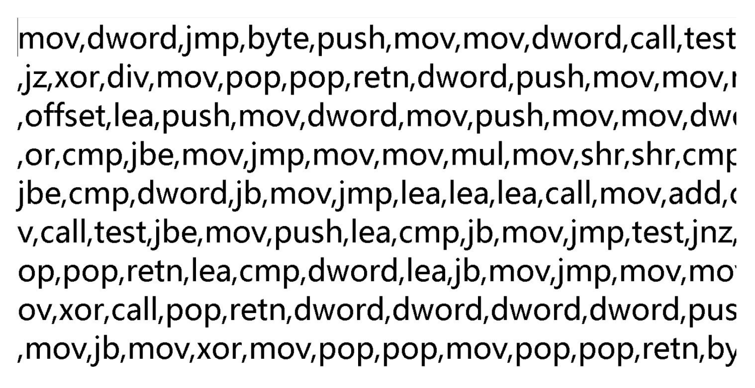
Figure 6 shows a sample of 0A32eTdBKayjCWhZqDOQ. The opcodes in each .asm file are sequentially extracted by regularization. The extracted opcode sequence text is shown in Figure 7.
The opcode sequences differ. Some are extremely long, so to extract more complete information, the method based on n-gram in natural language processing is used to extract the opcode features. By treating each opcode as a word, the n-gram method takes subsequences of the opcode sequence according to the magnitude of the n value with a sliding window, and then the frequency of the corresponding subsequence is calculated. Then, a word frequency threshold is set, and the subsequence with a particular number of occurrences above the threshold is retained. The retained subsequence is a feature of the malware.
- (2)
- Malware bytecode features
The malware itself is a file consisting of a series of bytes. One idea is to convert the binary file of malware into a grayscale image using the similarity between the values of the bytes and the range of pixel values taken in the grayscale image. The classification of malware families is achieved based on the texture similarity of grayscale images of the same family of malware and the different textures due to the different structures of different families of malware. To detect similar variants of malware, binary files can be better differentiated such that the impact of obfuscation is reduced.
Malware is converted into a sequence consisting of a binary, and the hexadecimal .byte file is read in binary, then divided by 16 bits in order, and converted into decimal values within [0, 256). The first line number of each byte file is ignored, and only the hexadecimal values after the line number are extracted. Only the values and letters in the byte file are kept, and the rest of the symbols are replaced with zeros, thus converting the malware file into a one-dimensional vector of decimal numbers.
The steps for extracting bytecode sequence features from malware are shown in Algorithm 1.
| Algorithm 1: The hex file is converted to a sequence of decimal values within [0, 256). |
| Input: hexadecimal file; |
| Output: a one-dimensional vector-matrix representation of file byte sequence. |
| 1. function getMatrixfrom(file) |
| 2. f = open(file,“rb”); /*read the file in binary */ |
| 3. /*convert binary file to a hexadecimal string */ |
| 4. /*convert the string to an unsigned decimal number by byte division into a byte*/ |
| 5. return byte; |
| 6. end function |
Similarly, the length of the sequence of each sample varies. To extract more complete information, intercept a particular length, then use each decimal number within that length as a feature, then calculate the frequency of each decimal value.
3.2. Feature Pre-Processing
After the malware features (opcode and bytecode features) were extracted, we checked whether this data had missing values, treated the missing values as 0 uniformly, and then performed standard normalization on the malware feature data. Data normalization reduced the variance of the features to a smaller interval, reduced the impact of the difference in the size of different feature values, and improved the convergence rate of the model. Current normalization methods are commonly used to normalize the values to (0,1) and (−1, 1). The normalization method used in this study was maximum-minimum normalization, which scales the values to the interval (0,1), as shown in Equation (5).
where is the scaled value, is the smallest value in the feature dimension, and is the largest value in the feature dimension.
In the process of malicious code feature extraction, there are many zero values. This method can retain the zeros in the features and can handle the data values with small variances in the features.
3.3. Combine TCN and BiGRU for Feature Extraction
The advantages of the TCN model are extraction of past data by one-dimensional causal convolution to guarantee temporality, time savings via the skip connect block, extraction of temporal features by dilated convolution, and the fusion of the average pooling layer with the maximum pooling layer. The advantage of using the GRU model is its nonlinear fitting ability to efficiently extract the data features and its faster convergence speed than the LSTM model [24]. The two-way GRU model better captures the sequence features of the opcode by collecting information forward and backward, thus improving the accuracy of model classification. These two models are integrated into the TCN-BiGRU model to obtain better accuracy as well as lower loss values. The structure of the integrated model is shown in Figure 8.
In Figure 8, the TCN-BiGRU model structure includes:
- Input layer: processed malicious code opcode feature data and shape (total number of samples, time step, and feature dimension).
- Time series convolutional network layer: the feature vectors were extracted via TCN, and the residual units were set up in two layers. A residual unit consisted of two convolutional units and one nonlinear mapping, and the convolutional kernel weights were normalized. The residual unit in Figure 8 was used only as the input layer to the hidden layer; the same was true for the hidden layer to the output layer. The convolution kernel size value was 4, and the dilation coefficient was (1, 2). Dropout was added to prevent overfitting in training.
- The different features extracted from the average pooling layer, as well as the maximum pooling layer, were fused as pooling outputs. We merged the average with the maximum pooling layer.
- The combined pooling layer consisted of a maximum pooling and an average pooling layer, each of which was calculated as shown in Equation (6). Maximum pooling and average pooling were obtained by traversing the pooling window with the input from the previous layer of the network. The pooled maximum and average values were then summed and passed to the next layer of the model structure.
- e.
- Bidirectional gated recurrent unit layer: The figure shows the structure of the GRU unit when it had two layers. The output vector of the TCN model was first used as the input of the GRU to extract the long-term correlation in the time series. Then the data were output with the results obtained from two layers of BiGRU.
- f.
- Output layer: Output the result of the last moment of the BiGRU to the classification layer.
3.4. Classification Output Layer
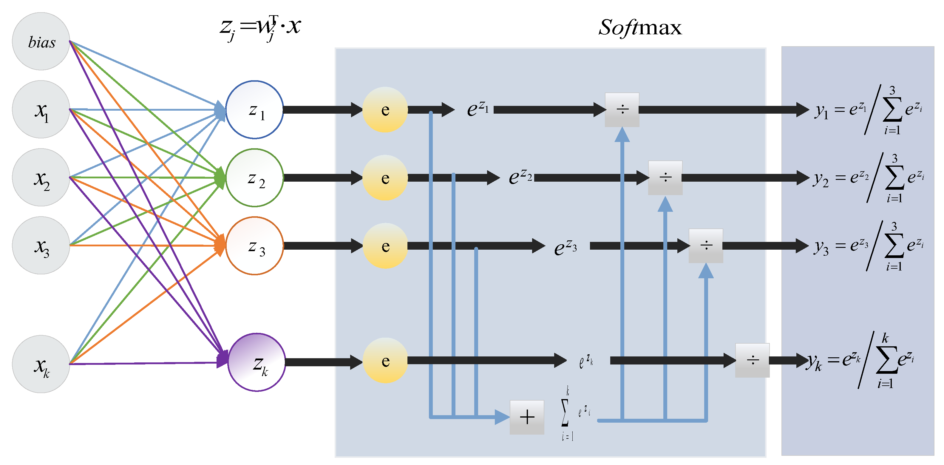
The classification output layer contained fully connected and softmax layers. The fully connected layer was used to obtain the display expression of the classification, and the softmax function was used to calculate the classification result of malicious code y. The structure of the classification output layer is shown in Figure 9.
The fully connected layer multiplied the weight matrix by the input vector and added a bias to map n (−∞, +∞) real numbers to K (−∞, +∞) real numbers (fractions); Softmax mapped K real numbers. The real numbers of (−∞, +∞) were mapped to K (0,1) real numbers (probabilities) while ensuring that their sum was 1.
where y denotes the probability of classification into malicious family type I; w denotes the weight matrix of the fully connected layer; and b is the bias vector of class i; at time t, replace x with .
The softmax layer superimposed the input features linearly with the weights. The number of neurons in the softmax layer was set by the number of malicious code types.
4. Experiments and Analysis of Results
4.1. Experimental Setup
To test the performance of the malicious code classification method fusing TCN and BiGRU, the following experiments were implemented:
Experiment 1: Feature selection experiment
Experiment 2: TCN-BiGRU model performance analysis experiment
Experiment 3: Comparison experiments of different pooling methods
Experiment 4: Model ablation comparison experiment
Experiment 5: Comparison experiments of different classification algorithms.
4.2. Experimental Environment and Data Set
The experimental environment was a computer configured with Win10, Intel Core (TM)-9880H CPU @ 2.30 GHz, 64 GB RAM, Quadro RTX 4000 GPU; the programming environment was PyCharm2021.2.2, using the Python 3.7 language in a CUDA 11.0 accelerated environment. The neural network model used TensorFlow 2.4.1 and Keras 2.4.3 versions of the deep learning framework.
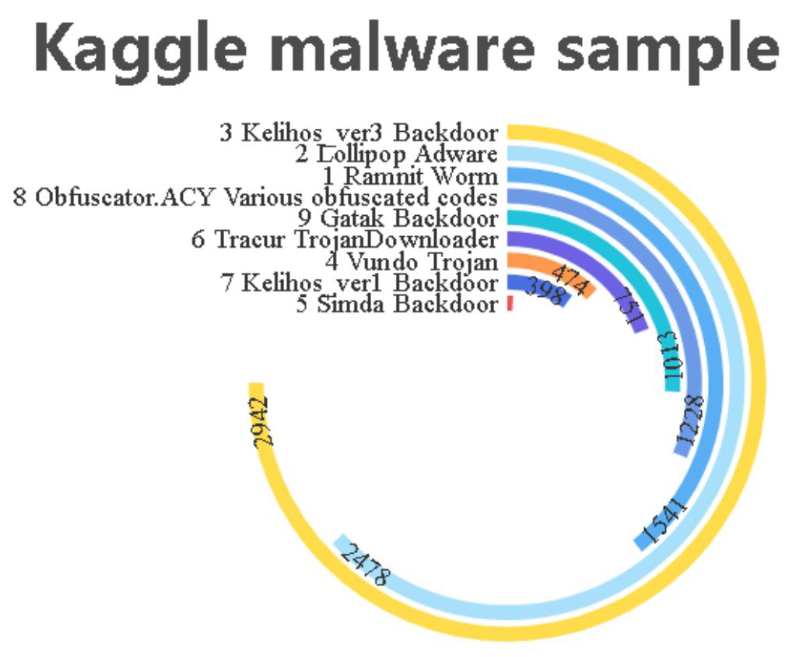
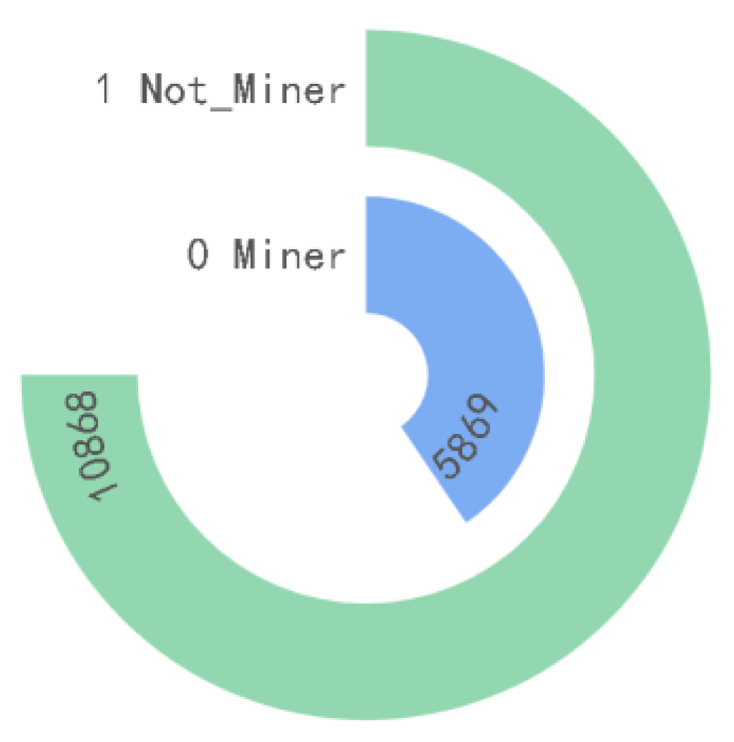
The experimental datasets were from the open-source dataset provided by Microsoft [15], and the PE samples were from the Datacon Open Data Project provided by Qianxin (China) [25]. The malicious code families in the dataset provided by Microsoft were divided into 9 categories, with 10,868 malware samples. Each sample file had two formats: .asm and .bytes; the PE samples provided by Qianxin had two categories, containing a large amount of mining-type malicious code and non-mining samples. These are the latest real samples captured from the existing network; thus, these samples are likely to contain a large number of shelling samples and resource obfuscation samples. To prevent samples’ mistaken execution from infecting the environment, the MZ and PE headers, as well as the import and export table parts, were removed. To ensure that the dataset samples have a certain level of diversity, similar samples were filtered. Therefore, in actual use, the MZ and PE headers were artificially added to extract the opcode features, and the samples were disassembled into .asm files using IDA tools. The family name, type number, number of samples, and expression number of the malware dataset used are shown in Figure 10 and Figure 11.
To fully evaluate our method, experiments were conducted on two different datasets according to different methods to fully validate the model. The first method used 9 malicious families in Kaggle malicious samples labeled 1–9, and the dataset was noted as 9-class-data. The second method used 0, 1 sub-table labeling on Datacon samples as sample labels, and the dataset was noted as 2-Class-Datacon; a five-fold cross-validation method was used to randomly divide the data into 10 parts, selecting 9 of these parts as the training set and 1 part as the test set.
4.3. Experimental Evaluation Criteria
The experiment selected common evaluation criteria in the field of malware classification detection: accuracy (Acc), precision (PR), recall (RR), and f1-score (F1) to evaluate the classification of the network. These criteria were calculated as follows:
where q is the number of samples; d is the number of categories; the value type is the processed one-hot code (string consisting of 0 or 1), and is the output value of the softmax function (). TP is the true class (meaning that malware was correctly classified as malware), FN is the false negative class (meaning that malware was incorrectly classified as normal software), FP is the false positive class (meaning that normal software was incorrectly classified as malware), and TN is the true negative class (meaning that normal software was correctly classified as normal software).
Model performance was presented using a visual representation of the confusion matrix, as shown in Table 2.
4.4. Feature Selection Experiments
After obtaining the opcode sequence, the n-gram method was used for feature extraction of the instruction file from the .asm file. The frequency f of the instruction n-gram in the .asm file was calculated as the feature and then used as input.
Normalization pre-processes the values of the frequency of the feature extracted from the n-gram of the malicious code, and the one-hot encoding method pre-processes the values of the malicious family categories. For example, the Ramnit family can be represented as 000000001.
In the experiment, the feature extraction was first performed by selecting N = 3, and then the instruction frequency threshold was selected as 300. Then, the test was conducted by increasing the value at 200 intervals, and the highest value selected was 1100. The experimental results showed that when instruction frequency increased, classification accuracy showed a trend of first rising and then decreasing, and the classification effect was best when the frequency was selected as 700, as shown in the lower panel of Figure 12.
In the experiments on change in the N value, the comparison experiment of N value was conducted using the frequency with the best effect in the instruction frequency experiment, i.e., a frequency of 700. As the N value increased, classification accuracy showed a trend similar to that of frequency, which also showed a trend of increasing and then decreasing. Through analysis of the experimental results, the classification effect was best at N = 3, and the experimental results are shown in the upper panel of Figure 13. Therefore, in subsequent experiments with the classification model, N = 3 was selected as the feature for input, and a frequency of 700 was selected as the input to the model.
For the byte code feature, the byte sequence with a length of fewer than 1500 bytes frequency was selected, then the experiment was conducted by increasing the frequency at an interval of 1000, and sequences with no more than 4500 in length were selected for the experiment. The experiment found that accuracy gradually decreased, so sequences within a length of 1000 were selected for training. The experiment then found that accuracy decreased compared to sequences within a length of 1500; thus, in subsequent features, we selected byte code with lengths below a 1500 bytes frequency for the fusion experiment.
4.5. TCN-BiGRU Model Performance Analysis Experiments
In the TCN-BiGRU model, the choice of some hyperparameters in the model could impact the experimental results. A single feature (n-gram method) was used in tuning the model to optimize model parameters. Two hyperparameters, the number of filters and the number of convolutional kernels, were selected among the optimization class parameters, and the number of BiGRU layers and the number of neurons per layer were selected as variables from the model class parameters. The number of model iterations was set at 50, the dilation coefficient in TCN was exponentially increased by 2, the dilation coefficient was set to (1, 2), the optimization algorithm was chosen as Adamax, and the learning rate was set at 0.002. To avoid the overfitting problem, a dropout layer was added, and the value was taken as 0.2. To make the experimental data more accurate and valid, a five-fold cross-validation method was used. The prediction data obtained from the experiments regarding the classification of malicious code families when setting a different number of filters, the number of convolutional kernels, and the number of neurons are shown in Table 3, Table 4 and Table 5, respectively.
Using the grid search algorithm, parameter search experiments were conducted for the filters (5, 7, 10, 15, 20) and the number of convolutional kernels (2, 3, 4, 5, 6) to finally determine the optimal parameter settings for the model, as shown in Table 4.
According to the values of each parameter obtained from the above experiments, the fusion of two features with N = 3, frequency = 700 and the first 1500 byte sequences was performed again using the TCN-BiGRU classification model.
The confusion matrix for the classification of the 9-class-data dataset is shown in Figure 14, with “Real label” on the vertical axis indicating true malicious code and “Prediction” on the horizontal axis indicating the prediction made by the model.
Table 5 shows in more detail the precision, recall, and FN-score (N = 1) of the predictions for each category. Note that for the Lollipop class, Vundo class, and Simda class, the classification is 100%. In the Kelihos_ver1 class, the classification is poor, with an accuracy of only 94%, while the remainder reached more than 99%. The family class Kelihos_ver1 belongs to the backdoor virus type in the broad category, while there are three families that are all backdoor viruses. Their poor classification was probably due to confusion with similar families.
Table 6 details the precision, recall, and fN-score (N = 1) for each category of predictions on the 2-Class-Datacon dataset. The table shows that the results were better for the Not_Miner classification on the 2-Class-Datacon dataset, with an accuracy greater than 96% and recall at 97%. The overall accuracy of the 2-Class-Datacon dataset was slightly worse, probably due to the presence of many shelled samples and resource confusion as this dataset was collected from the current network. As for whether model generalization ability was good on the 2-Class-Datacon dataset, model ablation was set, and different comparison tests were performed for verification.
4.6. Model Ablation Experiments
To verify the detection effect of the model proposed, model ablation experiments were performed. Under the same experimental conditions, TCN, GRU, TCN-GRU, and our model were compared on two different datasets to detect the corresponding results of each model for various indexes of the dataset. The detection results are shown in Table 6.
Observe from Table 7 that the proposed model significantly improved the classification effect of malicious samples, with accuracy up to 99.72% and 96.54% on the two datasets, respectively. The 9-Class-Datacon dataset has an accuracy improvement of 0.36%, 0.36%, and 0.18% using TCN, GRU, and TCN-GRU, respectively. The accuracy of the 2-Class-Datacon dataset was improved by 1.92%, 0.84%, and 1.02% using TCN, GRU, and TCN-GRU, respectively. Observing the results of the accuracy, completeness, and F1 values of the two datasets on the three models TCN, GRU, and TCN-GRU, it was found that the proposed TCN-BiGRU model outperformed TCN, GRU, and TCN-GRU in all indexes, thus verifying that the combination of both TCN and BiGRU in the model improved the detection effect for malicious code.
4.7. Comparison Experiments of Different Pooling Methods
To solve the problem of insufficient feature extraction abilities of the model, this study proposed a pooling fusion method that simultaneously averaged and maximized the pooling of data and performed parallel pooling. This section presents a comparison experiment on the effect of different pooling methods on the performance of malicious code classification. The model adopted four schemes: no pooling, average pooling, maximum pooling, and pooling fusion. The classification accuracy for both datasets is shown in Table 8.
From Table 8, observe that the method using pooling fusion has higher detection accuracy compared with schemes that perform average pooling or maximum pooling alone. By using pooling fusion to combine these two features and complement each other, we better reflected the nature of the network attack data and obtain higher identification accuracy. This experiment demonstrated that our pooling fusion method can significantly improve the ability of the model to extract features.
4.8. Comparison Experiments for Classification Algorithms
Regarding model performance, comparative experiments were conducted with reference to existing literature. Comparison experiments were done on the 9-Class-data dataset with reference to the relevant literature [9,10,26,27,28]. Experimental results are shown in Table 8. Among the five comparative studies, two focused on machine learning, one was related to gene sequence classification, and the remaining two concerned deep learning models. Burnaev et al. [26] used opcode features and grayscale map features, which were extracted and later detected by svm for classification. Narayanan et al. [27] processed grayscale graphs converted from malware, downscaling the features by PCA, and then classifying them using the machine learning model known as K nearest neighbor. Drew et al. [28] used a genetic detection method similar to Strand to classify text. Gibert et al. [10] extracted byte and opcode sequences, and then used a classifier composed of two CNNs for classification. Yan et al. [11] extracted features via a CNN model for grayscale maps and LSTM model for opcode features, then fused the results for classification. These methods produced good results, but there remained a gap between them and the method of this study. Under the accuracy evaluation criterion, our proposed TCN-BiGRU model integrating opcode and byte features achieved 99.72% accuracy; the accuracy values of the five comparison studies were all below 99.72%. Therefore, our proposed model incorporating both features and fusing TCN and BiGRU performed best.

Table 8.
9-class-data dataset_model comparison.
| Model | No Pooling | Average Pooling |
|---|---|---|
| One-class SVM [26] | Opcode + Grayscale map | 92% |
| PCA and kNN [27] | Grayscale map | 96.6% |
| Strand Gene Sequence [28] | Asm sequence | 98.59% |
| Orthrus [10] | Byte + Opcode | 99.24% |
| MalNet [11] | Opcode + Grayscale map | 99.36% |
| Model in this paper | Opcode + Byte | 99.72% |
For the 2-Class-Datacon dataset, we referred to the literature [29,30,31] to perform comparison experiments with the results shown in Table 9. Among these three comparison studies, one was on integration learning, one was on deep learning, and one was on machine learning. Guo et al. [29] extracted grayscale maps of malicious samples, extracts feature with different parameters for GIST descriptors, and then adopted the KNN and random forest algorithms to integrate classification by voting algorithm. Saadat et al. [30] also processed malicious sample images; it first pre-trained a good convolutional neural network model and then used the Xgboost algorithm for classification. Liu et al. [31] extracted the assembly instructions of malware samples. The assembly instructions were then pre-processed and downscaled using the LDA algorithm and were finally trained with the random forest algorithm for classification. These methods produced good results, but there remain gaps between them and the method proposed in this paper. Under the ACC evaluation criterion, our TCN-BiGRU model integrating opcode and byte features reached 96.54% accuracy; the ACC values of the three comparison papers were all under 96.54%. After the above comparative experiments on two datasets, it was proved that our proposed model integrating both features and fusing TCN and BiGRU performed best and had strong generalization capability.
5. Conclusions
Threats to cyberspace security are increasing, and classification of the massive number of viruses has become an increasingly critical issue. This study proposed a static classification model of malicious code fused with TCN and BiGRU to extract and integrate the opcode features and byte features of malicious code. The model focusd on the potential features of the data and obtained the long-term dependencies existing in the sequences through a BiGRU network in both directions. It showed several advantages, such as high classification detection rate, anti-shelling, and obfuscation on both datasets. It also showed good generalizability and adaptability to high data volume requirements. However, the method used for feature extraction was relatively simple and did not bring out the full performance of the features. In follow-up work, we will use a natural language classification model to further process the samples.
Author Contributions
X.W.: conceptualization, methodology, writing—original draft; Y.S.: formal analysis, writing—review and editing; Z.M.: conceptualization; X.H.: formal analysis; C.C.: methodology. All authors have read and agreed to the published version of the manuscript.
Funding
This work is supported by the National Science Foundation of China (61806219, 61703426 and 61876189), the National Science Foundation of Shaanxi Provence (2021JM-226), the Young Talent fund of the University and Association for Science and Technology in Shaanxi, China (20190108, 20220106), and the Innovation Capability Support Plan of Shaanxi, China (2020KJXX-065).
Institutional Review Board Statement
Not applicable.
Informed Consent Statement
Not applicable.
Data Availability Statement
All data used in this paper can be obtained by contacting the authors of this study.
Conflicts of Interest
The authors declare no conflict of interest.
References
- Zhao, J.; Zhang, S.; Liu, B.; Cui, B. Malware detection using machine learning based on the combination of dynamic and static features. In Proceedings of the 27th International Conference on Computer Communication and Networks (ICCCN), Hangzhou, China, 11 October 2018. [Google Scholar]
- Guo, H.; Wu, J.T.; Huang, S.G.; Pan, Z.L.; Shi, F.; Yan, Z.H. Research on malware detection based on vector features of assembly instructions. Inf. Secur. Res. 2020, 6, 113–121. [Google Scholar]
- Raff, E.; Sylvester, J.; Nicholas, C. Learning the pe header, malware detection with minimal domain knowledge. In Proceedings of the 10th ACM Workshop on Artificial Intelligence and Security; Association for Computing Machinery: New York, NY, USA, 2017; pp. 121–132. [Google Scholar]
- Zhao, S.; Ma, X.; Zou, W.; Bai, B. DeepCG: Classifying metamorphic malware through deep learning of call graphs. In Proceedings of the International Conference on Security and Privacy in Communication Systems; Springer: Berlin, Germany, 2019; pp. 171–190. [Google Scholar]
- Santos, I.; Brezo, F.; Ugarte-Pedrero, X.; Bringas, P.G. Opcode sequences as representation of executables for data-mining-based unknown malware detection. Inf. Sci. 2013, 227, 64–82. [Google Scholar] [CrossRef]
- Kang, B.; Yerima, S.Y.; McLaughlin, K.; Sezer, S. N-opcode Analysis for Android Malware Classification and Categorization. In Proceedings of the 2016 International Conference on Cyber Security and Protection of Digital Services (Cyber Security), London, UK, 9 July 2016. [Google Scholar]
- Pascanu, R.; Stokes, J.W.; Sanossian, H.; Marinescu, M.; Thomas, A. Malware classification with recurrent networks. In Proceedings of the 2015 IEEE International Conference on Acoustics, Speech and Signal Processing (ICASSP), South Brisbane, QLD, Australia, 19–24 April 2015; pp. 1916–1920. [Google Scholar]
- Kwon, I.; Im, E.G. Extracting the Representative API Call Patterns of Malware Families Using Recurrent Neural Network. In Proceedings of the International Conference on Research in Adaptive and Convergent Systems; Association for Computing Machinery: New York, NY, USA, 2017; pp. 202–207. [Google Scholar]
- Messay-Kebede, T.; Narayanan, B.N.; Djaneye-Boundjou, O. Combination of Traditional and Deep Learning based Architectures to Overcome Class Imbalance and its Application to Malware Classification. In Proceedings of the NAECON 2018-IEEE National Aerospace and Electronics Conference, Dayton, OH, USA, 23–26 July 2018; pp. 73–77. [Google Scholar]
- Gibert, D.; Mateu, C.; Planes, J. Orthrus: A Bimodal Learning Architecture for Malware Classification. In Proceedings of the 2020 International Joint Conference on Neural Networks (IJCNN), Glasgow, UK, 19–24 July 2020; pp. 1–8. [Google Scholar]
- Yan, J.; Qi, Y.; Rao, Q. Detecting malware with an ensemble method based on deep neural network. Secur. Commun. Netw. 2018, 2018, 7247095. [Google Scholar] [CrossRef] [Green Version]
- Narayanan, B.N.; Davuluru, V.S.P. Ensemble Malware Classification System Using Deep Neural Networks. Electronics 2021, 9, 721. [Google Scholar] [CrossRef]
- Ahmadi, M.; Ulyanov, D.; Semenov, S.; Trofimov, M.; Giacinto, G. Novel Feature Extraction, Selection and Fusion for Effective Malware Family Classification. In Proceedings of the 6th ACM Conference on Data and Application Security and Privacy; Association for Computing Machinery: New York, NY, USA, 2016; pp. 183–194. [Google Scholar]
- Zhang, Y.; Huang, Q.; Ma, X.; Yang, Z.; Jiang, J. Using Multi-features and Ensemble Learning Method for Imbalanced Malware Classification. In Proceedings of the 2016 IEEE Trustcom/BigDataSE/ISPA, Tianjin, China, 23–26 August 2016; pp. 965–973. [Google Scholar]
- Bai, J.R.; Wang, J.F. Improving malware detection using multiview ensemble learning. Secur. Commun. Netw. 2016, 9, 4227–4241. [Google Scholar] [CrossRef] [Green Version]
- Bai, S.; Kolter, J.Z.; Koltun, V. An empirical evaluation of generic convolutional and recurrent networks for sequence modeling. arXiv 2018, arXiv:1803.01271. [Google Scholar]
- Fan, Y.Y.; Li, C.J.; Yi, Q.; Li, B.Q. Classification of Field Moving Targets Based on Improved TCN Network. Comput. Eng. 2021, 47, 106–112. [Google Scholar]
- Yating, G.; Wu, W.; Qiongbin, L.; Fenghuang, C.; Qinqin, C. Fault Diagn-osis for Power Converters Based on Optimized Temporal Convolutional Network. IEEE Trans. Instrum. Meas. 2020, 70, 1–10. [Google Scholar] [CrossRef]
- Huang, Q.; Hain, T. Improving Audio Anomalies Recognition Using Temporal Convolutional Attention Network. In Proceedings of the ICASSP 2021 IEEE International Conference on Acoustics, Speech and Signal Processing (ICASSP), Toronto, ON, Canada, 6–11 June 2021; pp. 6473–6477. [Google Scholar]
- Zhu, R.; Liao, W.; Wang, Y. Short-term prediction for wind power based on temporal convolutional network. Energy Rep. 2020, 6, 424–429. [Google Scholar] [CrossRef]
- Xu, Z.; Zeng, W.; Chu, X.; Cao, P. Multi-Aircraft Trajectory Collaborative Prediction Based on Social Long Short-Term Memory Network. Aerospace 2021, 8, 115. [Google Scholar] [CrossRef]
- Liu, Y.; Ma, J.; Tao, Y.; Shi, L.; Wei, L.; Li, L. Hybrid Neural Network Text Classification Combining TCN and GRU. In Proceedings of the 2020 IEEE 23rd International Conference on Computational Science and Engineering (CSE), Guangzhou, China, 29 December–1 January 2020; pp. 30–35. [Google Scholar]
- Sun, Y.C.; Tian, R.L.; Wang, X.F. Emitter signal recognition based on improved CLDNN. Syst. Eng. Electron. 2021, 43, 42–47. [Google Scholar]
- Wang, Y.; Liao, W.L.; Chang, Y.Q. Gated Recurrent Unit Network-Based Short-Term Photovo-ltaic Forecasting. Energies 2018, 11, 2163. [Google Scholar] [CrossRef] [Green Version]
- Qi An Xin Technology Research Institute. DataCon: Multidomain Large-Scale Competition Open Data for Security Research. Available online: https://datacon.qianxin.com/opendata (accessed on 11 November 2021). (In Chinese).
- Burnaev, E.; Smolyakov, D. One-class SVM with privileged information and its application to malware detection. In Proceedings of the 2016 IEEE 16th International Conference on Data Mining Workshops (ICDMW), Barcelona, Spain, 12–15 December 2016; pp. 273–280. [Google Scholar]
- Narayanan, B.N.; Djaneye-Boundjou, O.; Kebede, T.M. Performance analysis of machine learning and pattern recognition algorithms for malware classification. In Proceedings of the 2016 IEEE National Aerospace and Electronics Conference (NAECON) and Ohio Innovation Summit (OIS), Dayton, OH, USA, 25–29 July 2016; pp. 338–342. [Google Scholar]
- Drew, J.; Hahsler, M.; Moore, T. Polymorphic malware detection using sequence classifcation methods and ensembles: BioSTAR 2016 Recommended Submission. EURASIP J. Inf. Secur. 2017, 2017, 2. [Google Scholar] [CrossRef]
- Guo, H.; Huang, S.; Zhang, M. Classification of malware variant based on ensemble learning. In International Conference on Machine Learning for Cyber Security; Springer: Cham, Switzerland, 2020; pp. 125–139. [Google Scholar]
- Saadat, S.; Joseph Raymond, V. Malware classification using CNN-Xgboost model. In Artificial Intelligence Techniques for Advanced Computing Applications; Springer: Singapore, 2021; pp. 191–202. [Google Scholar]
- Liu, Y.; Wang, Z.; Hou, Y. A method for feature extraction of malicious code based on probabilistic topic models. J. Compute. Res. Dev. 2019, 56, 2339–2348. [Google Scholar]
Figure 1.
Causal convolution.

Figure 2.
Dilated convolution.

Figure 3.
Residual block.

Figure 4.
Gated recurrent unit.

Figure 5.
Malware detection model structure.

Figure 6.
Original opcode sequence.

Figure 7.
Opcode sequence after pre-processing.

Figure 8.
TCN-BiGRU model.

Figure 9.
The classification output layer.

Figure 10.
Kaggle malware sample.

Figure 11.
Datacon sample.

Figure 12.
Experiment on the selection of N value and frequency.

Figure 13.
Sequence length selection experiment.

Figure 14.
Confusion matrix.

Table 1.
Operation codes.
| Category | Operation Codes |
|---|---|
| Data move | mov, movzx, push, pop, lea, xchg |
| Arithmetic/logic | add, sub, inc, dec, imul, or, xor, shl, shr, ror, rol |
| Control flow | jmp, jz, cmp, jnb, call, retf, retn |
| Other | nop |
Table 2.
Confusion Matrix.
| Location | Real Label | |
|---|---|---|
| For Malware | For Not Malware | |
| Malware | TP | FP |
| Not malware | FN | TN |
Table 3.
Parameter setting of model.
| Model Parameter | Real Label |
|---|---|
| Batch size setting | 64 |
| Optimizer | Adamax |
| Optimizer learning rate | 0.002 |
| Epoch setting | 50 |
| Number of TCN filters | 7 |
| Number of TCN convolution kernels | 4 |
| TCN dilation coefficient | (1, 2) cc |
| Number of BiGRU units | 32\32 |
| Dropout rate | 0.2 |
Table 4.
Parameter setting of model.
| Malicious Code Family | Precision | Recall | F1-Score |
|---|---|---|---|
| 1 | 0.99 | 1.00 | 1.00 |
| 2 | 1.00 | 1.00 | 1.00 |
| 3 | 0.99 | 1.00 | 1.00 |
| 4 | 1.00 | 1.00 | 1.00 |
| 5 | 1.00 | 1.00 | 1.00 |
| 6 | 0.99 | 1.00 | 0.99 |
| 7 | 0.94 | 1.00 | 0.97 |
| 8 | 0.99 | 0.99 | 0.99 |
| 9 | 0.99 | 0.99 | 0.99 |
| accuracy | - | - | 0.99 |
| Overall | 99.55% | 99.54% | 99.54% |
Table 5.
Parameter setting of model.
| Malicious Code Family | Precision | Recall | F1-Score |
|---|---|---|---|
| 0 | 0.94 | 0.93 | 0.93 |
| 1 | 0.96 | 0.97 | 0.96 |
| accuracy | - | - | 0.95 |
| Overall | 96.37% | 96.63% | 96.50% |
Table 6.
Ablation experiment of model.
| Model | Dataset | Accuracy | Precision | Recall | F1-Score |
|---|---|---|---|---|---|
| TCN | 9-class-data | 99.36% | 99.37% | 99.36% | 99.36% |
| 2-class-Datacon | 94.62% | 95.98% | 95.81% | 95.89% | |
| GRU | 9-class-data | 99.36% | 99.29% | 99.35% | 99.32% |
| 2-class-Datacon | 95.7% | 95.8% | 95.72% | 95.76% | |
| TCN-GRU | 9-class-data | 99.54% | 99.46% | 99.54% | 99.50% |
| 2-class-Datacon | 95.52% | 95.62% | 95.63% | 95.62% | |
| TCN-BiGRU | 9-class-data | 99.72% | 99.55% | 99.54% | 99.54% |
| 2-class-Datacon | 96.54% | 96.37% | 96.63% | 96.50% |
Table 7.
Accuracy for different pooling methods.
| Dataset | No Pooling | Average Pooling | Maximum Pooling | Pooling Fusion |
|---|---|---|---|---|
| 9-class-data | 99.45% | 99.54% | 99.45% | 99.72% |
| 2-class-Datacon | 94.92% | 95.10% | 95.28% | 96.54% |
Publisher’s Note: MDPI stays neutral with regard to jurisdictional claims in published maps and institutional affiliations. |
© 2022 by the authors. Licensee MDPI, Basel, Switzerland. This article is an open access article distributed under the terms and conditions of the Creative Commons Attribution (CC BY) license (https://creativecommons.org/licenses/by/4.0/).
Share and Cite
MDPI and ACS Style
Wu, X.; Song, Y.; Hou, X.; Ma, Z.; Chen, C. Deep Learning Model with Sequential Features for Malware Classification. Appl. Sci. 2022, 12, 9994. https://0-doi-org.brum.beds.ac.uk/10.3390/app12199994
AMA Style
Wu X, Song Y, Hou X, Ma Z, Chen C. Deep Learning Model with Sequential Features for Malware Classification. Applied Sciences. 2022; 12(19):9994. https://0-doi-org.brum.beds.ac.uk/10.3390/app12199994
Chicago/Turabian StyleWu, Xuan, Yafei Song, Xiaoyi Hou, Zexuan Ma, and Chen Chen. 2022. "Deep Learning Model with Sequential Features for Malware Classification" Applied Sciences 12, no. 19: 9994. https://0-doi-org.brum.beds.ac.uk/10.3390/app12199994
Note that from the first issue of 2016, this journal uses article numbers instead of page numbers. See further details here.