

Improving Streaming Video with Deep Learning-Based Network Throughput Prediction

Department of Computer Networks and Systems, Silesian University of Technology, Akademicka 16, 44-100 Gliwice, Poland
Appl. Sci. 2022, 12(20), 10274; https://0-doi-org.brum.beds.ac.uk/10.3390/app122010274
Submission received: 15 September 2022
/
Revised: 7 October 2022
/
Accepted: 9 October 2022
/
Published: 12 October 2022
(This article belongs to the Special Issue Advance in Digital Signal, Image and Video Processing)
Abstract
:Video streaming represents a significant part of Internet traffic. During the playback, a video player monitors network throughput and dynamically selects the best video quality in given network conditions. Therefore, the video quality depends heavily on the player’s estimation of network throughput, which is challenging in the volatile environment of mobile networks. In this work, we improved the throughput estimation using prediction produced by LSTM artificial neural networks (ANNs). Hence, we acquired data traces from 4G and 5G mobile networks and supplied them to two deep LSTM ANNs, obtaining a throughput prediction for the next four seconds. Our analysis showed that the ANNs achieved better prediction accuracy compared to a naive predictor based on a moving average. Next, we replaced the video player’s default throughput estimation based on the naive predictor with the LSTM output. The experiment revealed that the traffic prediction improved video quality between 5% and 25% compared to the default estimation.
1. Introduction
Highly variable packet delays, packet losses and fluctuating mobile network bandwidth make streaming a video challenging. Although modern mobile networks offer high bandwidth, the nature of wireless transmission—inherent variability in signal strength, interference, noise, and user mobility—results in high throughput variability. To overcome this unstable network environment, content providers encode video into multiple versions at different bit rates and split them into segments. A video player periodically downloads the segments, concatenates them and delivers a continuous video stream to a user. During the playback, the player can request a different version of the segments to adapt the video bit rate to the current network conditions. This video delivery concept is called dynamic adaptive streaming over HTTP (DASH).
The rate-adaptation algorithm is a significant element of a DASH system because the player has to estimate network conditions, including available throughput to ensure proper quality of experience (QoE). The measurement of network throughput, usually based on the moving average, often differs from real throughput. Because of this difference, streaming algorithms can be too conservative and download a video of much lower quality than the throughput allows, or too aggressive and download content of too high quality in given network conditions. A solution to this problem is to predict the future network throughput. As the video segment is usually several seconds long, the prediction is short-term and does not rely on seasonality. Prediction can improve the efficiency of bit rate selection, which translates to lower startup delay and offers better mid-stream bit rate adaptation. Researchers estimate that the applied prediction achieves between 68% and 89% of the optimal quality. The exact numbers are dependent on the playback algorithms employed in a DASH player [1].
In our work, we predict throughput using traces from 4G and 5G networks from static and mobile usage scenarios. In the next step, we replace the default methods of throughput estimation in three DASH algorithms with the obtained predicted results. Finally, we show that the DASH algorithms achieve better performance when equipped with prediction compared with reliance only on an average of network measurements. Our approach does not require any modification to network protocols or the DASH standard and its components. The solution only affects users’ players where a more elaborate algorithm based on LSTM artificial neural networks (ANNs) replaces the default throughput estimation. With the information provided by the player’s measurement module, the algorithm can estimate the expected throughput for the next few seconds. Because an LSTM ANN requires some computation needed to learn and continually update its knowledge, this process increases the usage of memory and CPU of a video player.
Taking the above into account, the contributions of the paper are: the prediction of 5G network throughput at the application level in static and mobile scenarios; the comparison of the prediction quality with the 4G trace; the usage of stacked uni- and bidirectional LSTM ANNs versions for the prediction, and the application of the prediction made by an LSTM ANN to improve quality of video for three DASH players.
In the next section, we describe the related works. In Section 3, we present the video streaming model, adaptation strategies of video playback and video quality measurement. Section 4 shows the prediction model, LSTM ANNs, used for the prediction, data characteristics, prediction results and the prediction influence on the video quality. The last section concludes the paper.
2. Related Works
The literature on network throughput prediction is extensive and usually focuses on the Internet traffic, which aggregates flows generated by a whole spectrum of applications. The authors of [2] show a comprehensive review of prediction methods and compare some of them. A number of research studies used linear regression, autoregressive integrated moving average (ARIMA), ARIMA with an explanatory variable (ARIMAX), multiple linear regression, support vector regression, GARCH processes and many other techniques derived from statistics. These methods are conventionally called traditional and are considered descriptive in nature, aimed at analyzing datasets with finite, countable, and explainable predictors. The authors of [3] made a comprehensive comparison of the traditional methods using a 3G/HSPA data set.
The newer prediction schemes based on machine learning are sometimes used in accordance or opposition to the traditional methods, and there is an ongoing debate about their accuracy and computational requirements [4]. ANNs, considered a non-traditional approach, play a role in network traffic prediction mainly due to their universality and accuracy. Historically, the popularity gained simple ANNs with a single hidden layer because versions with multiple layers, called deep ANNs, were harder to train. After researchers overcame the training issues, deep ANNs became popular and gradually replaced single-layered ANNs as a tool for the solution of more complex problems. Because deep ANNs added more complexity and nonliterary to the network traffic model, their prediction accuracy increased. Oliveira’s comparative study [5] discusses both approaches in the context of network traffic prediction.
From the variety of deep ANNs, LSTM ANNs are one of the possible choices and are applied readily due to their capability to capture long-range dependencies characteristic of aggregated network traffic, i.e., traffic composed of multiple flows. For example, an LSTM ANN was used to identify recurrent patterns of various metrics to predict traffic in cellular networks in [6]. The work focuses on long-horizon prediction counted in days. In [7], the authors enhanced their LSTM-based prediction with an autocorrelation function, which captured the traffic cycles on a daily scale with a prediction span between 5 and 60 min. In [8], the authors proposed to remove extreme values by scaling a traffic trace. Their LSTM ANN had four hidden layers with a time window set to 32 units or more. The authors did not provide a prediction horizon; however, the data granularity was more than one minute.
In the case of multimedia applications, the prediction of a single traffic flow is more important and challenging than aggregated traffic [9]. A single flow, especially if transmitted through an unstable mobile environment, can have much variability and sudden changes compared with an aggregated trace smoothed by statistical multiplexing. Hence, the models of the aggregated traffic are usually not suitable for describing a single flow generated by a DASH system streaming video segments in an ON–OFF fashion, which contributes to significant bursts in the transmission. As single-flow prediction is a more challenging task, there are fewer works dedicated to this topic, and their authors focus mainly on a short-time prediction span. In [10], the authors applied LSTM and gated recurrent units (GRU) ANNs to predict traffic flow obtained from a sensor network for a five-minute time horizon. They achieved better results compared with the ARIMA processes. A comparative study [11] showed that for cellular network traffic, LSTM provides better prediction than a stacked autoencoder. Unfortunately, the authors did not provide information about the traffic traces used in the experiment.
Except for the historical throughput, an LSTM ANN sometimes operates on additional data to improve the results; for example, the authors of [12] used a complex LSTM ANN with five hidden layers and a multivariate dataset containing information about all downlink and uplink traffic for a given base station. Other works use a meta-learning scheme, including a set of predictors, each optimized to predict a particular kind of traffic. The study by He et al. [9] applied this technique to improve traffic scheduling in base stations with a prediction horizon set to 100 ms. The authors of [13] stated that, for the prediction of flow throughput, the best result was achieved by a random forest technique, which outperformed a deep ANN. They tested different time windows spanning from 0.03s to 4s on nearly 1 million flows containing traces from miscellaneous networks and applications. In addition to flow history data, the study used other attributes related to TCP: window size, window scale or segments retransmissions. Azari et al. in [14] analyzed the effect of different parameters of an LSTM ANN and ARIMA on prediction accuracy. The simulation demonstrated the superiority of LSTM over ARIMA, especially for longer time series. The paper [15] employs the same methods and concludes that historical traffic is the most important feature when predicting future network throughput. However, the authors also state that relying only on the throughput alone leads to worse performance compared to the methods using more inputs. Another short-term prediction is proposed in [16], where He et al. evaluated the ARIMA and LSTM for the prediction of both single and multiple flows taking into account video and non-video traffic. Using a prediction span between 10 and 100 ms, they found that LSTM ANNs achieved good results at the cost of more training computations.
DASH algorithms usually implement a simple throughput prediction based on an average of past measurements. Advanced solutions try to optimize video playback by employing more elaborate prediction techniques. Some researchers state that the playback algorithms fed with an accurate estimation of network throughput outperform those that do not apply predictive methods, while others observe that prediction alone is not sufficient and should be combined with other techniques, e.g., buffer control [1]. In [17], the authors focus on inaccuracies in throughput measurements occurring due to idle periods between the chunks causing sub-optimal adaptation decisions. The authors show that a simple prediction scheme based on adaptive filtering can improve the quality of the streaming video. Raca et al. in [18] compared several prediction schemes, among them support vector machines, random forest and LSTM ANN, and applied them to a single DASH algorithm. Interestingly, the authors reported that a DASH player supported by the best predictor achieved nearly the same performance as in the case of the ideal prediction. In addition to application data, the model relied on network data, reaching as deep as the physical layer, which may be a reason behind the extraordinary high accuracy of the prediction. To improve the video quality, in [19], the authors propose active queue management (AQM). The AQM uses LSTM to predict the router’s queue delay, which temporarily stores DASH packets. Increasing queue delay triggers removal of the packets in the queue. This, in turn, forces traffic sources to reduce their transmission rate and induces a video player to decrease the video-bit rate before the network stalls, which allows for smoother video playback. In [20], we proposed employing (F)ARIMA processes, shallow ANNs and an recursive auto-encoder to enhance the performance of a DASH system.
In this work, we operate on traces gathered from 4G and 5G networks. To date, the analysis of the traffic generated by the latter network has limited coverage in the literature. We rely only on application-level throughput measurements; therefore, the proposed solution does not require modifications to network infrastructure or the TCP stack. Consequently, our work shows the impact of the prediction on video QoE without the support of any other information, which is hard to gather and requires profound changes in a DASH system. Contrary to the majority of the works, which aim at either short or long time horizons, our prediction span is 4 s, which is suitable for a DASH system.
3. Theoretical Background
3.1. Video Streaming Model
We model the video stream as a set of consecutive data segments , where is the amount of data measured in bytes and . Every segment contains L seconds of video encoded with a given bit rate; hence, the total length of the video is seconds. A video player obtains from a server a video segment encoded with a bit rate (bit/s), where and are the lower and upper bound, respectively, of the bit rate levels. A user considers a video with a higher bit rate as having better quality compared to its lower bit rate version.
A video player downloads video segments and places them in its buffer, where they wait for a playback. At the time , the player starts to download the video segment . Its downloading time is a function of the bit rate and averaged network throughput . At the time , the video player completes the download of the segment . At time , where , the video player starts to download the next segment . At the time , the player’s buffer stores time units of video. The maximum buffer capacity depends on the video player implementation. If (bit/s) is the average network throughput at time , then:
where
During the video playback, the amount of data in the player’s buffer fluctuates. The buffer increases by L seconds after a player downloads the segment , while it decreases when a user watches the video. Hence, the evolution of the buffer is described as:
If , the buffer becomes empty, which freezes the video.
3.2. Adaptation Strategies
At the time , a video player, which has only information of the past network throughput , selects the bit rate . To estimate the future throughput , the player may use a predictor defined as . Except the throughput, a player may also take into account its buffer level. Having the information about the network and a buffer state, the player selects the next segment quality, see Figure 1, as follows:
In our work, we presented three exemplary methods of the video bit rate selection. The first method is based on the simplified version of the algorithm implemented in the MSS video player, which is described in [21]. The second approach employs the implementation of ExoPlayer—a video player for Android developed by Google [22]. The third solution is described in [23], and we will further refer to it as Tian2016.
The first algorithm selects a video bit rate as follows
The buffer-based part of the algorithm selects the video bit rate considering the player’s buffer state. When the buffer level reaches , the system increases the bit rate (2a) by one level, denoted as . Similarly, when the playback drains the buffer below the threshold (2b), the player reduces the video quality by one level, denoted as . When the buffer level is between the thresholds and , the player estimates throughput and selects a corresponding quality level. If the estimated throughput is lower than the video bit rate , the player decreases video quality (2c). The bit rate remains unchanged (2d), when the estimated throughput is not sufficiently high. In the case when the bit rate surpasses the throughput by at least d bits/s, the player increases the video quality (2e). The parameter d marks a stripe of the throughput for which the player continues to download videos of the same quality. Hence, the parameter d stabilizes video quality and prevents frequent switches, which degrades content reception. The constants and define the lowest and the highest bit rates of video segments. We implemented this idea in the open-source software dash.js [24] and presented it in Figure 2. Taking the experiment’s parameters from [25], we set the player’s buffer size to 35 s and the thresholds and to 40% and 80% of the buffer size.
The second algorithm is a part of the ExoPlayer library. Its input parameters are a buffer size and throughput estimation. The algorithm calculates the video quality that fits in the currently available bandwidth according to the formula:
The algorithm scans the available qualities Q and selects the representation with the highest average bit rate lower than or equal to the estimated throughput r modified by a factor , as presented in (3a). The algorithm will switch to the best achievable video bit rate if it differs from the current bit rate, excluding two scenarios: network throughput increases but the buffer level remains low (3b) or network throughput decreases but the buffer level remains high (3c). For ExoPlayer, the default values for and are 10 and 25 s.
The third algorithm, which we will refer to as Tian2016, avoids video bit rate variability resulting from throughput fluctuations and estimation errors. Additionally, when the available network bandwidth remains higher for a longer time than the current video bit rate, the algorithm increases the video bit rate steadily and decreases it more aggressively when the throughput falls. A proportional-integral-derivative (PID) controller is responsible for the player’s decision regarding video bit rate selection. A PID implements a control loop with a feedback mechanism, which transfers the controller’s output value to the system input. The system adjusts its output by computing the difference between a set point and a measured process variable. The authors claim that their algorithm quickly responds to congestion level shifts and maintains a stable video rate during throughput variations. We took the parameters for the algorithm from [23] from sections V and VI-D.
As was stated earlier, a DASH system fragments a video into segments. The segment length L is usually between 2 and 10 s; for example, the MSS algorithm uses 2–5 s [25]. In our work, we set the video segment length to 4 s.
3.3. Quality Measures
DASH systems strive to achieve the best possible QoE by selecting optimal video bit rates in given network conditions. This selection involves a few conflicting issues. Firstly, a user expects that the streaming video will have the highest possible bit rate available for the given network throughput. Secondly, the playback should be smooth, which a player achieves by avoiding frequent bit rate changes. Thirdly, a player should minimize the times when the video freezes on a user’s screen due to the player’s buffer depletion. Having identified the three main components of QoE, namely bit rate, bit rated variation and rebuffering time, we combine them into a single measure, where the QoE is calculated as a weighted sum of the parameters of each video segment in the range from 1 to N:
where and are positive weights corresponding to video quality variations and rebuffering time. To count the buffer’s starvation periods, we introduce the penalty function and .
Video stalls disturb users more than bit rate switches do; thus, the value of is usually much higher than . A small indicates that bit rate switches are less nuisance for a user, while a large implies that the user is more concerned about rebuffering.
To obtain time- and video-independent measures with possibilities of comparison with different algorithms, we adapt from [26] a normalized QoE model
where QoE_ref is the QoE of another benchmark algorithm.
4. Prediction of Network Throughput
4.1. The Prediction Problem
We have measurements of the past throughput , and we are to predict the value of . Hence, we use a predictor , which takes the past throughput
The problem is to choose , which minimizes the difference between and .
Typically, a DASH algorithm predicts network throughput for the nearest future , using an average of past throughput measurements [27]
According to [28], DASH players apply the estimator (6) or its variation based on weighted, exponential or harmonic moving average. In our work, we improve the estimation by replacing the simple computation (6) with an LSTM ANN.
To measure the accuracy of the prediction algorithm, we chose the normalized root mean square error (NRMSE)
The NRMSE represents the squared difference between predictions and observed values divided by the number of observations N. An average of observed values normalizes the calculation result. The lower the NRMSE value, the better the model describes empirical data. The normalization allows us to compare predictions among traces with different throughput levels.
4.2. Long Short-Term Memory Networks
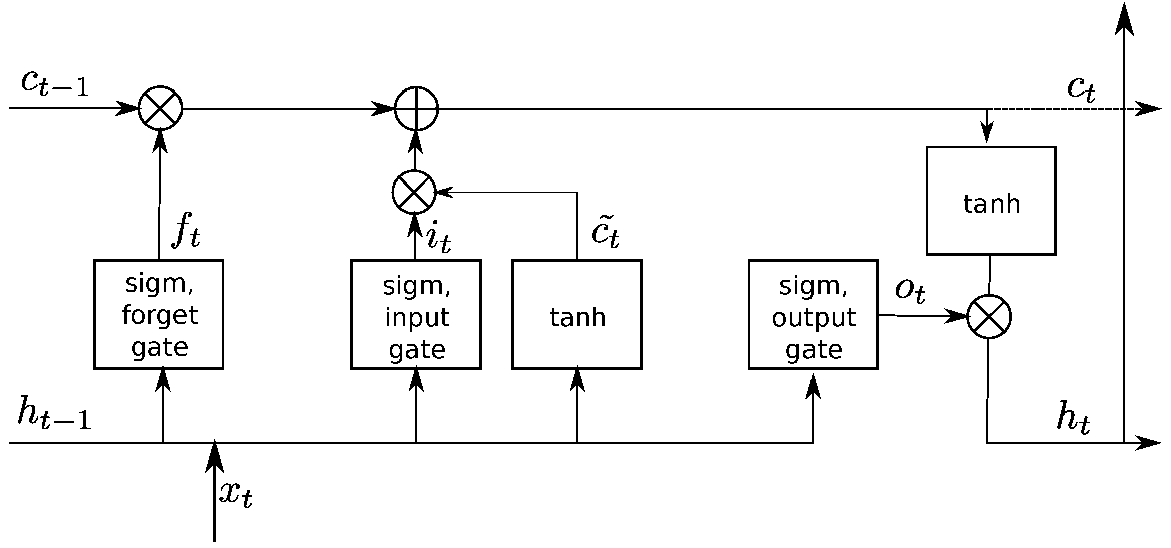
An LTSM is a recurrent ANN, which can learn long-range dependencies in data. LSTM ANNs respond to the short-term memory problem of recurrent ANNs. Namely, a recurrent ANN has difficulties retaining data from earlier computations because it misses information about long-memory dependencies. An LSTM ANN handles this problem by allowing its memory cells to select when to forget certain information, thus achieving the optimal time lags for time series problems. For this purpose, a network uses a memory block, which contains cells with self-connections, memorizing the temporary state and three adaptive, multiplicative gates (input, output and forget) to control information flow in the block—see Figure 3. The gates can learn to open and close, enabling LSTM memory cells to store data over long periods, which is desirable in time series prediction with long temporal dependency. Multiple memory blocks form a hidden layer. An LSTM ANN consists of an input layer, at least one hidden layer and an output layer.
An LSTM’s cell takes three inputs and generates two outputs:
where is an element of time series, is a cell’s memory signal from the previous time , and is a cell’s output signal at the previous time . At the time t, the cell generates two signals: —a cell’s state and —a cell’s output, which is passed to an upper ANN layer.
At every time step, the element of a time sequence enters the cell. Both output signals and leave the cell at time t and return to that same cell at a time . The cell can multiply or add signals, which are denoted by the symbols × and +. Cell gates also use two functions: sigm and tanh. The first represents the sigmoid function, which outputs numbers between zero and one (), describing how much of each signal to let through. The value of zero transfers nothing, while a value of one transfers everything. The second function represents the hyperbolic tangent ) and denotes which fraction of the candidate value updates the cell’s state .
An entering signal simultaneously reaches all three cell’s gates. The forget gate decides which part of the memory from the previous state transfers to the current state. The gate multiplies the signal using its weight and projects it into a unit interval using a sigmoid function
The remaining two gates determine which new information to store in the cell. Firstly, the input gate decides which values to update, transforming them into a unit interval. Next, the tanh layer creates a new candidate value and adds it to the cell state later.
Finally, the new state replaces the old one : the old state multiplies the forget gate value , and the candidate result multiplies the input gate value
Equation (8) controls the amount of information , which will form the state of the cell at the time t.
In the cell’s right-side, a multiplicative operation generates the output signal
which is the product of the actual memory signal computed in (8) and the signal
generated in the output gate. The output signal describes how much information the cell transmits to other cells at the next time point.
For our study, we use two architectures: stacked and sequence to sequence. The differences between these architectures are described in [29].
4.2.1. Stacked Unidirectional LSTM
An ANN can consist of multiple hidden layers, which include LSTM cells. In such a case, the output of one hidden layer is fed as the input into the subsequent hidden layer. Such deep ANN architecture allows progressively building up a higher level of representations of sequence data and mapping more complex, non-linear dependencies, which a single-layered, shallow network does not discover.
A special case is stacked architecture, where a hidden layer is multiplied and stacked on top of each other, creating a grid of cells, as shown in Figure 4. Cells composing the grid share their connections’ weights and biases. The outputs are forwarded as inputs to the next immediate layer above. The top layer produces , which corresponds to the expected unprocessed forecasts for the input time series. Each step of a training process calculates training error and accumulates it until the end of the time series , where is the actual value of the time series.
4.2.2. Stacked Bidirectional LSTM
A time series provided to an LSTM ANN is arranged chronologically: the information is passed in a positive direction from the time step to the time step t along the chain-like structure. However, it is also possible to process sequence data in both forward and backward directions. This idea is utilized in Bidirectional LSTM (BdLSTM) ANNs, which connect two hidden layers: a forward LSTM layer and a backward LSTM layer, to the same output layer, as illustrated in Figure 5. Thus, a BdLSTM ANN considers additionally backward dependencies, which pass information in a negative direction from the time step t to . This allows a BdLSTM ANN to capture more patterns, which a unidirectional LSTM could filter. The BdLSTM ANN computes its forward layer output iteratively from the positive sequence’s inputs from time to . Using the reversed inputs from time to , the BdLSTM calculates the backward layer output .
The standard LSTM updating method based on the equations presented in Section 4.2 computes both forward and backward layer outputs. A BdLSTM layer generates an output , calculated as
where the function is used to combine the two output sequences. Similar to the LSTM layer, the final output of a BdLSTM layer can be represented by , which is an expected unprocessed forecast.
Figure 5.
Bidirectional architecture of an LSTM network. BdLSTMs apply both forward and backward dependencies.
Figure 5.
Bidirectional architecture of an LSTM network. BdLSTMs apply both forward and backward dependencies.

4.3. Traffic Characteristics
The traffic traces were collected in Ireland by a large telecommunication operator. They include static and mobility scenarios and total roughly 21 h. We divided them into four sets: 5G, 4G, static and mobile, as listed in Table 1. A more detailed description of the traffic generation, capture methodology and properties of the traces can be found in [30] for 4G and in [31] for the 5G traffic.
Table 1 shows that the average rates of the 5G traces are about 50% higher than 4G traces for the static scenario. Furthermore, the 5G traces achieve nearly three times higher variation rates, reaching about 25 MB/s, compared to 4G traces, which obtain 9.6 MB/s. In the mobile scenario, the differences between 5G and 4G are lower—the average throughput of 5G traces is only 27% higher than the 4G traces. The authors of [30] explain these differences by the lack of 5G base stations across the driving routes where the traffic was captured. Despite this restriction, the upper limit for the variation range is still almost two times higher for 5G than 4G.
We use (1) to denote an average amount of traffic registered within a specified time. The length of a video segment is L, as stated in Section 3.1. A video player downloads segments at the rate ; hence, the player measures network throughput roughly every L seconds. In our model, we assumed .
4.4. Traffic Prediction with an LSTM ANN
For the time series prediction, an LSTM ANN uses a sliding window containing n most recent observations, as defined in (5). From every set of the traces listed in Table 1, we extracted ten overlapping sub-traces every 30 min. The models were trained on the first 10 min of each sub-trace and tested on its remaining part. We concatenated the obtained predictions, which allowed us to input their values into a video player and have uninterrupted playback.
For the prediction, we used a many-to-one architecture, where a throughput sequence is ANN’s input, and a single throughput value is a prediction. Firstly, we normalize the traffic flow sequence , i.e., remove trends and differentiate it obtaining , which is then delivered to the LSTM ANN. Both our LSTMs, unidirectional and bidirectional, consist of an input, two hidden and output layers. The top LSTM layer supplies its output to a conventional feed-forward ANN, which maps them into a single value that corresponds to an unprocessed prediction at time . Finally, we denormalize the output values from the feed-forward ANN, obtaining the prediction of network throughput at . This process and the structure of the LSTM ANN used for predicting traffic flow are presented in Figure 6.
An LSTM ANN minimizes the NRMSE defined in (7) through training, which iteratively changes the weights and biases of the network to decrease the differences between the model output and observed values. For this purpose, we chose Backpropagation Through Time (BPTT) algorithm. The BPTT unfolds an LSTM ANN and converts it into a feed-forward ANN to apply the backpropagation algorithm. Then, the backpropagation algorithm finds the gradient of the cost taking network parameters as the input, which in the case of an LSTM are the same for every unfolded time step. The algorithm aggregates the errors from the unfolded time steps, updates the weights and folds the ANN back. Due to good performance, relative simplicity and implementation in popular software, the BPTT is popularly used for the RNN ANNs, including their LSTM variants. More information about the algorithm and its comparison with others can be found in [32].
4.5. Model Validation
The prediction is more accurate for traces generated by static terminals compared with the mobile ones; see Figure 7. Furthermore, the traffic from 4G systems obtained a lower NRMSE than the 5G traces. These differences may result from the positive correlation between the prediction errors and variance of the traces. The traces generated by mobile scenarios have higher variation than the static ones, see Table 1. Additionally, the 5G traces, due to higher network bandwidth, achieved higher peak values. The variation of the results is roughly on the same level, except for the 5G mobile scenario where the NRMSEs have a higher range. Compared to a simple moving average, the LSTM predictions achieved lower NRMSE. The difference is particularly notable for the mobile and 5G scenarios. In all scenarios, the best result was obtained by the BdLSTM.
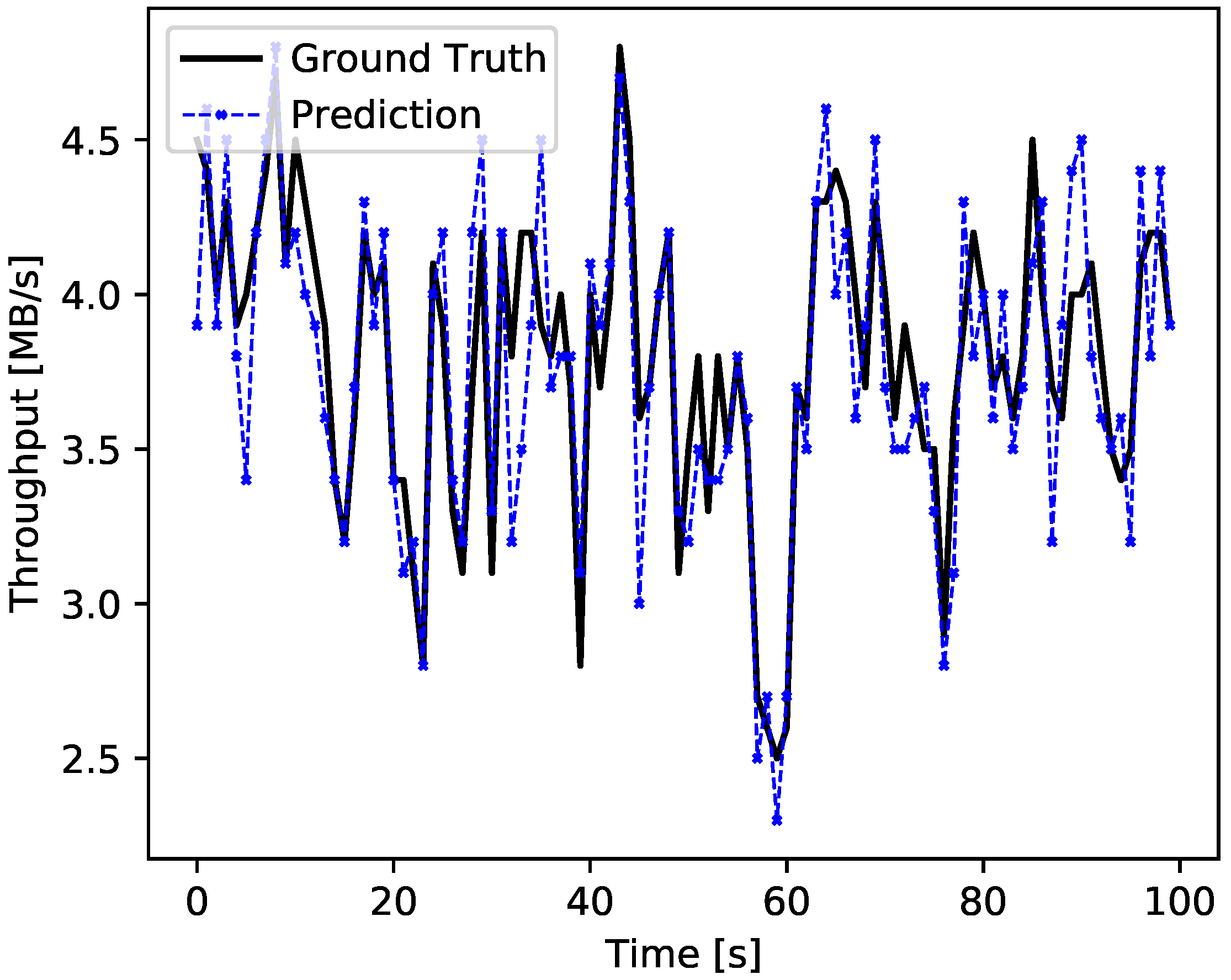
In Figure 8, we presented a fragment of the M5G trace to visualize the traffic characteristics and the prediction accuracy. The trace has an irregular structure without clearly identifiable patterns. The traffic frequently and abruptly changes its volume, producing oscillations between 2.5 and 5 MB/s. The prediction generally follows the traffic pattern relatively well; however, sometimes, it overestimates the scope of the oscillations, especially in the fragments where the traffic fluctuations have a higher frequency.
The prediction errors for the exemplary M5G trace have a normal distribution with a zero mean, as shown in Figure 9a. The errors are between −1.0 and 1.0 MB/s, and most do not exceed 0.5 MB/s. Compared with the case of the simple moving average shown in Figure 9b, its histogram is broader, and consequently, the errors have higher values than for the LSTM prediction.
Figure 8.
One-step prediction for the M5G trace. The prediction tends to overestimate the traffic oscillations, but the unidirectional LSTM ANN achieves better results than a naive predictor based on a simple moving average.
Figure 8.
One-step prediction for the M5G trace. The prediction tends to overestimate the traffic oscillations, but the unidirectional LSTM ANN achieves better results than a naive predictor based on a simple moving average.

Figure 9.
Distribution of prediction errors generated by (a) the unidirectional LSTM and (b) a simple moving average for the one-step prediction for M5G trace. The narrower prediction error interval for the LSTM ANN indicates fewer errors and better prediction accuracy.
Figure 9.
Distribution of prediction errors generated by (a) the unidirectional LSTM and (b) a simple moving average for the one-step prediction for M5G trace. The narrower prediction error interval for the LSTM ANN indicates fewer errors and better prediction accuracy.

4.6. Playback Algorithms Supported by Prediction
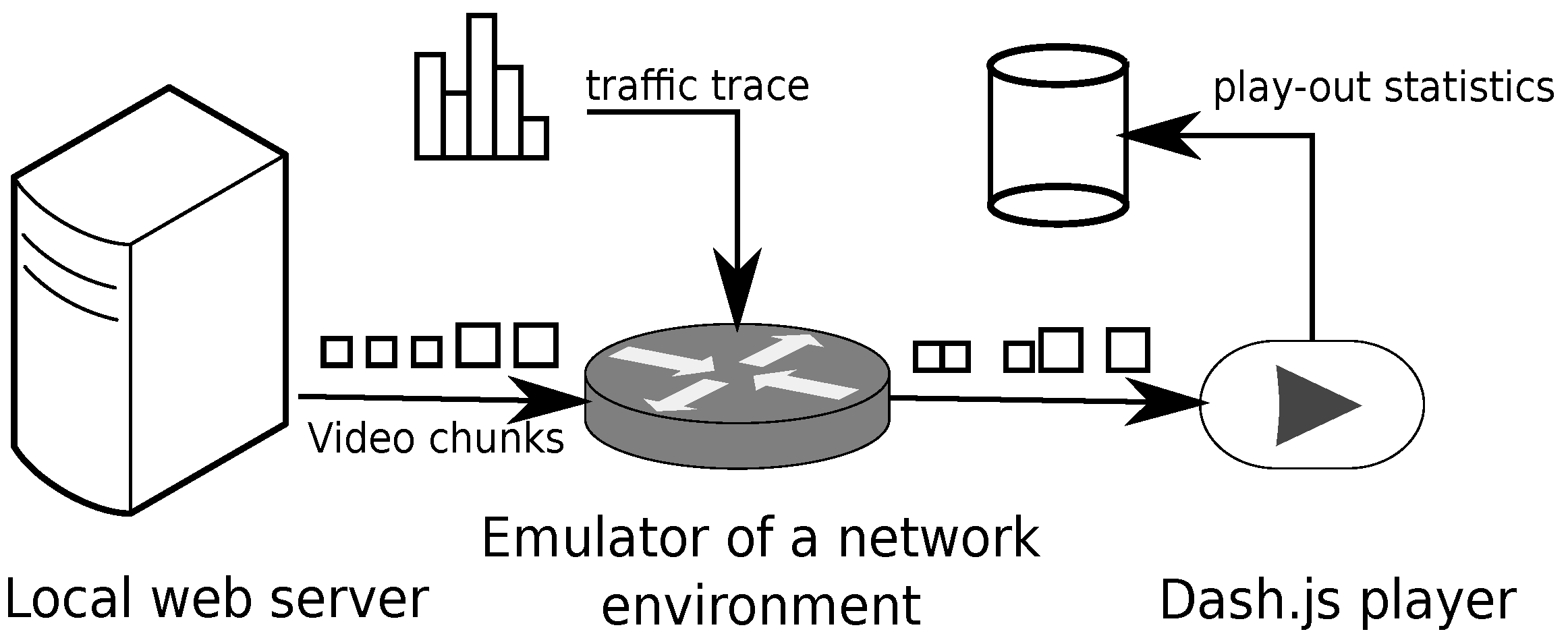
To assess the influence of the prediction on the quality of the video, we prepared a local media streaming system consisting of three Linux machines, as illustrated in Figure 10. The first machine ran a web server, the second one ran a traffic control facility netem, and the last one ran the dash.js player [24] in a Google Chrome browser. To emulate a mobile network, we used the netem module, which gave us control over bandwidth, packet delay and loss. For our experiments, we used the traffic from mobile environments examined in Section 4.3 as a network capacity trace, set a uniformly distributed delay from an interval [5 ms, 145 ms] and set a uniformly distributed packet loss from an interval [0.05%, 0.15%]. We placed six video files acquired from [33] at the web server and encoded them with 18 bit rates ranging from 0.1 to 20 MB/s. The server streamed the video to dash.js media player, which has an open-source code, which allows for the implementation and comparison of different playback algorithms.
The predicted throughput may integrate into the adaptation logic in two different ways. Firstly, it is possible to incorporate a prediction algorithm directly into a DASH player and replace its default throughput estimation algorithm. This approach requires translating the model into a native DASH player’s code or wrapping the model into a package, which the player calls an external dependency. In summary, it requires deep integration into the player’s implementation, which is challenging. In the second case, the prediction overwrites the measured throughput samples. The player acquires the information about throughput not directly from a network but from an output of the prediction model. This solution is easier to implement as it only requires minimal amendment of the player’s code; hence, we replaced the default throughput estimation with the predicted values, see Figure 11. As we mentioned in Section 3.2, we also overwrote the default playback algorithm implemented in the plug-in using the simplified versions of MSS, ExoPlayer and Tian algorithms.
Figure 12 shows a fragment of the performance of the MSS algorithm in its original version and the modified version with the support of the prediction made by a unidirectional LSTM. Both versions operate on the M5G trace from the set presented in Table 1. Compared with the original version, the prediction-supported algorithm switches its bit rates less often and more quickly recovers from bandwidth drops; nevertheless, its average bit rate is similar. Consequently, the less frequent switching of bit rates in the prediction-based version does not come at the cost of a lower bit rate.
Figure 13 compares nQoE (4) between the LSTM prediction and simple moving average. The nQoE is higher from about 5% to over 20%, depending on a DASH player and streaming scenario. In the case of MSS and ExoPlayer, the average improvement is mostly between 10% and 15%. For static traces generated by the 4G system, this value is closer to 10%; for mobile scenarios, the improvement is about 17%. The mobile use case obtains better results on average, but the higher nQoE variation indicates that the refinement is not uniform but depends on network conditions. Throughput in mobile scenarios, especially involving the 5G network, has higher variability (see Table 1); therefore, some parts of the traces may be harder to predict. The poorer performance of the default prediction based on moving average can also contribute to better relative improvement. For Tian, the resulting pattern is similar, but the gain is a few percent lower than in the other two algorithms. The more complex algorithm based on a PID controller and less reliance on direct throughput estimation probably reduces the benefits of the prediction. Comparing the LSTM versions, the algorithms with support of the BdLSTM have slightly better scores for the MSS and ExoPlayer algorithms. In the case of Tian, the results are roughly the same.
4.7. Discussion of the Results
Our analysis shows that an LSTM ANN obtains better prediction accuracy compared with a naive predictor based on a moving average. The prediction achieved the best results for traffic registered by fixed terminals. The traffic acquired from mobile equipment, especially that operating on a 5G network, had a more irregular structure and was harder to predict for both the LSTM ANN and a moving average. However, for mobile traces, the accuracy of the prediction made by the moving average deteriorates even faster than the accuracy of an LTSM ANN. From the two LSTM versions we tested, the BdLSTM shows slightly better prediction accuracy compared to the unidirectional LSTM. Although we used an NRMSE (7), comparison with other research is not easy, as their NRMSE values differ significantly across different works. For instance, in [9], the NRMSE ranges between about 0.1 and 5.5 depending on an LSTM ANN and a data set used for the prediction, whereas in [12], the NRMSE is below 0.1 for all experiments. It is also unclear how the authors normalized their errors as they did not specify explicit mathematical formulas in their works. In other mentioned works in Section 2, e.g., [6,7,8,10], the authors provided non-normalized and non-comparative mean square error measures of prediction errors. Sometimes this measure is normalized as in [34] (normalized mean absolute error) or [13] (relative MSE) but is non-comparative with NRMSE without additional data.
Exemplary DASH algorithms supported by throughput prediction achieved better performance than their versions with default throughput estimators. Most gained the MSS and ExoPlayer playback strategies, while the results for Tian were lower. An explanation is the degree of complexity of the examined approaches. The first two algorithms rely heavily on rate estimation and use for this purpose moving averages, while the buffer measurements play a supportive role. In the case of Tian, the algorithm uses primarily the buffered video time as a feedback signal, while the expected throughput is estimated using support vector regression. This shift of focus results in a lower impact of prediction on the algorithm performance.
To our best knowledge, there is only a single work with which we can directly compare the results because every research uses its own set of measures. In our work, the quality improvement is between 5% and 25%, while for the perfect throughput prediction, Raca et al. [35] reached 55% using a similar nQoE (4) measure. The authors built a perfect estimator by looking explicitly into the future values of time series and applied it to three algorithms: ExoPlayer, Elastic [36] and Arbiter+ [37]. Similarly to our case, the simpler algorithm ExoPlayer profited the most from the prediction. The prediction gave a less impressive nQoE increase for the two other, more complex algorithms.
5. Conclusions
In this work, we improved the performance of adaptive streaming algorithms employing LSTM ANNs that predicted network throughput. As a result, the system provides higher video quality without longer buffering times or a higher frequency of bit rate changes. The improvement is more significant in 5G networks; nevertheless, advanced playback algorithms gain less from throughput prediction. The best results achieved relatively simple strategies based on throughput and buffer measurement. The improvement is not uniform across the usage scenario and depends on network conditions. The prediction gain was smaller for a more complex playback algorithm supported by the proportional-integral-derivative controller. From the two tested LSTM versions, the bidirectional LSTM gained a slightly better prediction score.
Our approach does not require modifications of the network infrastructure or the TCP stack. Unlike proprietary solutions, DASH has an open specification and leaves the implementation of the playback logic to third parties; thus, our solution can be integrated with adaptation algorithms. The prediction model relies only on past throughput measurement and works without additional network information, which can be hard to acquire. Therefore, the prediction accuracy and the quality improvement are less impressive than in some cited works, which support their prediction with additional data.
We identified several potential paths for further investigation. Firstly, the traffic models can be improved, as some authors report that the best results are usually obtained by hybrid techniques. It will be interesting to investigate how to leverage the additional information to increase the prediction accuracy, as more elaborate approaches may better adjust to network data and provide better input for adaptive algorithms. Secondly, there is room to extend our prediction beyond the current single video chunk horizon. Thirdly, one can investigate the optimal length of the training, test sets and a time horizon that provides the best prediction. Finally, we would like to move from the offline analysis to an online prediction made by a mobile device, which measures the throughput in real-time and provides information about battery, memory and processor usage.
Funding
The work was carried out within the statutory research project of the Department of Computer Networks and Systems.
Institutional Review Board Statement
Not applicable.
Informed Consent Statement
Not applicable.
Data Availability Statement
Publicly available datasets were analyzed in this study. The data can be found here https://www.ucc.ie/en/misl//research/datasets/ivid_4g_lte_dataset/ (accessed on 5 October 2022) and here https://github.com/uccmisl/5Gdataset (accessed on 5 October 2022).
Conflicts of Interest
The authors declare no conflict of interest.
References
- Zou, X.K.; Erman, J.; Gopalakrishnan, V.; Halepovic, E.; Jana, R.; Jin, X.; Rexford, J.; Sinha, R.K. Can Accurate Predictions Improve Video Streaming in Cellular Networks? In Proceedings of the 16th International Workshop on Mobile Computing Systems and Applications, ACM, Santa Fe, NM, USA, 12–13 February 2015; pp. 57–62. [Google Scholar]
- Katris, C.; Daskalaki, S. Comparing forecasting approaches for Internet traffic. Expert Syst. Appl. 2015, 21, 8172–8183. [Google Scholar] [CrossRef]
- Liu, Y.; Lee, J.Y. An Empirical Study of Throughput Prediction in Mobile Data Networks. In Proceedings of the 2015 IEEE Global Communications Conference (GLOBECOM), San Diego, CA, USA, 6–10 December 2015; pp. 1–6. [Google Scholar]
- Makridakis, S.; Spiliotis, E.; Assimakopoulos, V. Statistical and Machine Learning forecasting methods: Concerns and ways forward. PLoS ONE 2018, 13, e0194889. [Google Scholar] [CrossRef] [PubMed] [Green Version]
- Oliveira, T.P.; Barbar, J.S.; Soares, A.S. Computer network traffic prediction: A comparison between traditional and deep learning neural networks. Int. J. Big Data Intell. 2016, 3, 28–37. [Google Scholar] [CrossRef]
- Dalgkitsis, A.; Louta, M.; Karetsos, G.T. Traffic forecasting in cellular networks using the lstm rnn. In Proceedings of the 22nd Pan-Hellenic Conference on Informatics, Athens, Greece, 29 November–1 December 2018; pp. 28–33. [Google Scholar]
- Zhuo, Q.; Li, Q.; Yan, H.; Qi, Y. Long short-term memory neural network for network traffic prediction. In Proceedings of the 2017 12th International Conference on Intelligent Systems and Knowledge Engineering (ISKE), Nanjing, China, 24–26 November 2017; pp. 1–6. [Google Scholar] [CrossRef]
- Alsaade, F.W.; Hmoud Al-Adhaileh, M. Cellular Traffic Prediction Based on an Intelligent Model. Mob. Inf. Syst. 2021, 2021, 6050627. [Google Scholar] [CrossRef]
- He, Q.; Moayyedi, A.; Dan, G.; Koudouridis, G.P.; Tengkvist, P. A Meta-Learning Scheme for Adaptive Short-Term Network Traffic Prediction. IEEE J. Sel. Areas Commun. 2020, 38, 2271–2283. [Google Scholar] [CrossRef]
- Fu, R.; Zhang, Z.; Li, L. Using LSTM and GRU neural network methods for traffic flow prediction. In Proceedings of the 2016 31st Youth Academic Annual Conference of Chinese Association of Automation (YAC), Wuhan, China, 11–13 November 2016; pp. 324–328. [Google Scholar] [CrossRef]
- Cao, S.; Liu, W. LSTM Network Based Traffic Flow Prediction for Cellular Networks. In Simulation Tools and Techniques; Song, H., Jiang, D., Eds.; Springer International Publishing: Cham, Switzerland, 2019; Volume 295, pp. 643–653. [Google Scholar] [CrossRef]
- Trinh, H.D.; Giupponi, L.; Dini, P. Mobile traffic prediction from raw data using LSTM networks. In Proceedings of the 2018 IEEE 29th Annual International Symposium on Personal, Indoor and Mobile Radio Communications (PIMRC), Bologna, Italy, 9–12 September 2018; pp. 1827–1832. [Google Scholar]
- Labonne, M.; López, J.; Poletti, C.; Munier, J.B. Short-Term Flow-Based Bandwidth Forecasting using Machine Learning. arXiv 2020, arXiv:2011.14421. [Google Scholar]
- Azari, A.; Papapetrou, P.; Denic, S.; Peters, G. Cellular traffic prediction and classification: A comparative evaluation of LSTM and ARIMA. In Proceedings of the International Conference on Discovery Science, Split, Croatia, 28–30 October 2019; pp. 129–144. [Google Scholar]
- Yue, C.; Jin, R.; Suh, K.; Qin, Y.; Wang, B.; Wei, W. LinkForecast: Cellular Link Bandwidth Prediction in LTE Networks. IEEE Trans. Mob. Comput. 2018, 17, 1582–1594. [Google Scholar] [CrossRef]
- He, Q.; Koudouridis, G.P.; Dán, G. A comparison of machine and statistical time series learning for encrypted traffic prediction. In Proceedings of the 2020 International Conference on Computing, Networking and Communications (ICNC), Big Island, HI, USA, 17–20 February 2020; pp. 714–718. [Google Scholar]
- Bentaleb, A.; Timmerer, C.; Begen, A.C.; Zimmermann, R. Performance Analysis of ACTE: A Bandwidth Prediction Method for Low-latency Chunked Streaming. ACM Trans. Multimed. Comput. Commun. Appl. 2020, 16, 1–24. [Google Scholar] [CrossRef]
- Raca, D.; Zahran, A.H.; Sreenan, C.J.; Sinha, R.K.; Halepovic, E.; Jana, R.; Gopalakrishnan, V. On Leveraging Machine and Deep Learning for Throughput Prediction in Cellular Networks: Design, Performance, and Challenges. IEEE Commun. Mag. 2020, 58, 11–17. [Google Scholar] [CrossRef]
- Santos, C.E.M.; da Silva, C.A.G.; Pedroso, C.M. Improving Perceived Quality of Live Adaptative Video Streaming. Entropy 2021, 23, 948. [Google Scholar] [CrossRef] [PubMed]
- Biernacki, A. Traffic prediction methods for quality improvement of adaptive video. Multimed. Syst. 2018, 24, 531–547. [Google Scholar] [CrossRef] [Green Version]
- Zambelli, A. IIS Smooth Streaming Technical Overview; Microsoft Corporation: Albuquerque, NM, USA, 2009. [Google Scholar]
- ExoPlayer. 2022. Available online: https://github.com/google/ExoPlayer (accessed on 5 October 2022).
- Tian, G.; Liu, Y. Towards Agile and Smooth Video Adaptation in HTTP Adaptive Streaming. IEEE/ACM Trans. Netw. 2016, 24, 2386–2399. [Google Scholar] [CrossRef]
- (DASH-IF). JavaScript Reference Client. 2022. Available online: https://reference.dashif.org/dash.js/ (accessed on 5 October 2022).
- Famaey, J.; Latré, S.; Bouten, N.; Van de Meerssche, W.; De Vleeschauwer, B.; Van Leekwijck, W.; De Turck, F. On the merits of SVC-based HTTP adaptive streaming. In Proceedings of the Integrated Network Management (IM 2013), Ghent, Belgium, 27–31 May 2013; pp. 419–426. [Google Scholar]
- Belda, R.; de Fez, I.; Arce, P.; Guerri, J.C. Look ahead to improve QoE in DASH streaming. Multimed. Tools Appl. 2020, 79, 25143–25170. [Google Scholar] [CrossRef]
- Li, Z.; Zhu, X.; Gahm, J.; Pan, R.; Hu, H.; Begen, A.C.; Oran, D. Probe and adapt: Rate adaptation for http video streaming at scale. IEEE J. Sel. Areas Commun. 2014, 32, 719–733. [Google Scholar] [CrossRef] [Green Version]
- Bentaleb, A.; Taani, B.; Begen, A.C.; Timmerer, C.; Zimmermann, R. A Survey on Bitrate Adaptation Schemes for Streaming Media Over HTTP. IEEE Commun. Surv. Tutorials 2019, 21, 562–585. [Google Scholar] [CrossRef]
- Hewamalage, H.; Bergmeir, C.; Bandara, K. Recurrent Neural Networks for Time Series Forecasting: Current Status and Future Directions. Int. J. Forecast. 2021, 37, 388–427. [Google Scholar] [CrossRef]
- Raca, D.; Quinlan, J.J.; Zahran, A.H.; Sreenan, C.J. Beyond throughput: A 4G LTE dataset with channel and context metrics. In Proceedings of the 9th ACM Multimedia Systems Conference, Amsterdam, The Netherlands, 12–15 June 2018; pp. 460–465. [Google Scholar] [CrossRef]
- Raca, D.; Leahy, D.; Sreenan, C.J.; Quinlan, J.J. Beyond throughput, the next generation: A 5G dataset with channel and context metrics. In Proceedings of the 11th ACM Multimedia Systems Conference, Istanbul, Turkey, 8–11 June 2020; pp. 303–308. [Google Scholar] [CrossRef]
- Shrestha, A.; Mahmood, A. Review of Deep Learning Algorithms and Architectures. IEEE Access 2019, 7, 53040–53065. [Google Scholar] [CrossRef]
- Zabrovskiy, A.; Feldmann, C.; Timmerer, C. Multi-codec DASH dataset. In Proceedings of the 9th ACM Multimedia Systems Conference, Amsterdam, The Netherlands, 12–15 June 2018; pp. 438–443. [Google Scholar] [CrossRef]
- Kim, M. Network traffic prediction based on INGARCH model. Wirel. Netw. 2020, 26, 6189–6202. [Google Scholar] [CrossRef]
- Raca, D.; Zahran, A.H.; Sreenan, C.J.; Sinha, R.K.; Halepovic, E.; Jana, R.; Gopalakrishnan, V.; Bathula, B.; Varvello, M. Incorporating Prediction into Adaptive Streaming Algorithms: A QoE Perspective. In Proceedings of the 28th ACM SIGMM Workshop on Network and Operating Systems Support for Digital Audio and Video, Amsterdam, The Netherlands, 12–15 June 2018; pp. 49–54. [Google Scholar] [CrossRef]
- De Cicco, L.; Caldaralo, V.; Palmisano, V.; Mascolo, S. ELASTIC: A client-side controller for dynamic adaptive streaming over HTTP (DASH). In Proceedings of the 2013 20th International Packet Video Workshop, San Jose, CA, USA, 12–13 December 2013; pp. 1–8. [Google Scholar]
- Zahran, A.H.; Raca, D.; Sreenan, C.J. Arbiter+: Adaptive rate-based intelligent http streaming algorithm for mobile networks. IEEE Trans. Mob. Comput. 2018, 17, 2716–2728. [Google Scholar] [CrossRef]
Figure 1.
Adaptation strategy for video. A video player chooses the quality of video, taking into account the prediction of network throughput and its buffer state.
Figure 1.
Adaptation strategy for video. A video player chooses the quality of video, taking into account the prediction of network throughput and its buffer state.

Figure 2.
An example operation of a simplified version of the MSS algorithm. At times and , network throughput is high enough to increase the video bit rate (2e). At , the buffer level, which is above the threshold, allows increasing the video bit rate again (2a). At times and , network throughput drops, which causes the video bit rate to decrease (2c). At time , the buffer level drops below the threshold, and the video bit rate is reduced again (2b). After , network throughput is not high enough to increase the video-bit rate (2d).

Figure 3.
Structure of LSTM memory block: is an input signal at the time t, and represent cell states at the previous and actual t times, and are output signals of the cell at and t times, b represents the bias. The symbol × represents the multiplication and + summation of signals.
Figure 3.
Structure of LSTM memory block: is an input signal at the time t, and represent cell states at the previous and actual t times, and are output signals of the cell at and t times, b represents the bias. The symbol × represents the multiplication and + summation of signals.

Figure 4.
Stacked architecture—a hidden layer is multiplied and stacked on top of each other creating a grid of cells.
Figure 4.
Stacked architecture—a hidden layer is multiplied and stacked on top of each other creating a grid of cells.

Figure 6.
Architecture of the LSTM ANN used for network throughput prediction.

Figure 7.
NRMSE of the analyzed prediction models for different traces. Every box on the plot represents predictions made on ten overlapping sub-traces every 30 minutes, which were extracted from traces listed in Table 1.
Figure 7.
NRMSE of the analyzed prediction models for different traces. Every box on the plot represents predictions made on ten overlapping sub-traces every 30 minutes, which were extracted from traces listed in Table 1.

Figure 10.
Experiment setup includes a web server, the netem module and the dash.js video player. The connection between the emulated network and the server has fixed parameters. The netem module shapes the traffic between the emulated network and the DASH player, providing variable transmission time of video segments.

Figure 11.
The architecture of the dash.js reference player. The modified estimation module acquires information about network throughput from the LSTM ANN. The MSS, ExoPlayer and Tian algorithms replaced the player’s default playback logic.
Figure 11.
The architecture of the dash.js reference player. The modified estimation module acquires information about network throughput from the LSTM ANN. The MSS, ExoPlayer and Tian algorithms replaced the player’s default playback logic.

Figure 12.
Performance of MSS algorithm without and with support of traffic prediction. Throughput prediction eliminates some of the video bit rate drops observed at the beginning, end and approximately the 20th min of the trace. However, as the prediction sometimes overestimates the throughput, the bit rate unnecessarily switches to a higher level at about the 20th min of the trace.

Figure 13.
The relative improvement of the nQoE metric across different HAS algorithms and network traces with respect to the no-prediction: (a) MSS, LSTM, (b) ExoPlayer, LSTM, (c) Tian, LSTM, (d) MSS, BdLSTM, (e) ExoPlayer, BdLSTM, and (f) Tian, BdLSTM. The nQoE metrics are normalized to the no-prediction case set to 0% improvement. The scenarios with traces from the mobile environment obtain, on average, better results, but their variation is also higher.


Publisher’s Note: MDPI stays neutral with regard to jurisdictional claims in published maps and institutional affiliations. |
© 2022 by the author. Licensee MDPI, Basel, Switzerland. This article is an open access article distributed under the terms and conditions of the Creative Commons Attribution (CC BY) license (https://creativecommons.org/licenses/by/4.0/).
Share and Cite
MDPI and ACS Style
Biernacki, A. Improving Streaming Video with Deep Learning-Based Network Throughput Prediction. Appl. Sci. 2022, 12, 10274. https://0-doi-org.brum.beds.ac.uk/10.3390/app122010274
AMA Style
Biernacki A. Improving Streaming Video with Deep Learning-Based Network Throughput Prediction. Applied Sciences. 2022; 12(20):10274. https://0-doi-org.brum.beds.ac.uk/10.3390/app122010274
Chicago/Turabian StyleBiernacki, Arkadiusz. 2022. "Improving Streaming Video with Deep Learning-Based Network Throughput Prediction" Applied Sciences 12, no. 20: 10274. https://0-doi-org.brum.beds.ac.uk/10.3390/app122010274
Note that from the first issue of 2016, this journal uses article numbers instead of page numbers. See further details here.