

Structure-Function Coupling Reveals Seizure Onset Connectivity Patterns
by
 , ,
, ,
Christina Maher
1,2,* ,
,
Arkiev D’Souza
2,3,
Michael Barnett
2,4,5,
Omid Kavehei
1,
Chenyu Wang
2,3,5 and
Armin Nikpour
4,6 1
School of Biomedical Engineering, Faculty of Engineering, The University of Sydney, Darlington, NSW 2008, Australia
2
Brain and Mind Centre, The University of Sydney, Camperdown, NSW 2050, Australia
3
Translational Research Collective, Faculty of Medicine and Health, The University of Sydney, Camperdown, NSW 2050, Australia
4
Department of Neurology, Royal Prince Alfred Hospital, Camperdown, NSW 2050, Australia
5
Sydney Neuroimaging Analysis Centre, Camperdown, NSW 2050, Australia
6
Central Clinical School, Faculty of Medicine and Health, The University of Sydney, Camperdown, NSW 2050, Australia
*
Author to whom correspondence should be addressed.
Appl. Sci. 2022, 12(20), 10487; https://0-doi-org.brum.beds.ac.uk/10.3390/app122010487
Submission received: 15 September 2022
/
Revised: 7 October 2022
/
Accepted: 12 October 2022
/
Published: 18 October 2022
(This article belongs to the Special Issue Advances in Neuroimaging Data Processing)
Abstract
:The implications of combining structural and functional connectivity to quantify the most active brain regions in seizure onset remain unclear. This study tested a new model that may facilitate the incorporation of diffusion MRI (dMRI) in clinical practice. We obtained structural connectomes from dMRI and functional connectomes from electroencephalography (EEG) to assess whether high structure-function coupling corresponded with the seizure onset region. We mapped individual electrodes to their nearest cortical region to allow for a one-to-one comparison between the structural and functional connectomes. A seizure laterality score and expected onset zone were defined. The patients with well-lateralised seizures revealed high structure-function coupling consistent with the seizure onset zone. However, a lower seizure lateralisation score translated to reduced alignment between the high structure-function coupling regions and the seizure onset zone. We illustrate that dMRI, in combination with EEG, can improve the identification of the seizure onset zone. Our model may be valuable in enhancing ultra-long-term monitoring by indicating optimal, individualised electrode placement.
1. Introduction
The assessment of patients with focal epilepsy using a combination of structural data derived from diffusion MRI (dMRI) and functional data from electroencephalography (EEG) is gaining increased appeal [1,2,3]. In the brain, structural connectivity refers to an anatomical link between two or more brain regions. Connnectomes generated from diffusion MRI, can represent the strength of structural connectivity between specific brain regions. Functional connectivity is inferred from the spatio-temporal relationship between electrophysiological signals from two or more structurally discrete regions [4]. Structural connectivity is believed to give rise to functional and network behaviour [5]. In a mechanistic sense, the composition of white matter can be expected to influence the flow of activity and connectivity between neuronal populations. Therefore, if EEG functions as a tool to observe the flow of activity, the connectivity measurements from EEG can be presumed to closely resemble connectivity measurements from structural MRI. In epilepsy, structure-function coupling is proposed to have a role in identifying seizure propagation patterns [6,7], seizure generalisation [1] and predicting post-surgery seizure freedom [8,9]. Diffusion MRI derived tractography, in conjunction with EEG, can enable the quantification of structural connectivity between different brain regions. However, in epilepsy, dMRI is held to be in the experimental realm [2]. Therefore, though there is consensus on the significance of structural connectivity information in patient diagnosis, the utility of dMRI as a routine clinical test has not been realised. Additional research is needed to investigate the value of dMRI in combination with routinely collected data such as EEG. Further, the feasibility of user-friendly tools for deploying dMRI pipelines must be assessed.
Several works employ functional MRI (fMRI) to represent functional connectivity [10,11,12] alongside structural connectivity from dMRI. However, given EEG is routinely collected in epilepsy clinics, it may be a more accessible and practical alternative to fMRI, which has inherent, poor temporal resolution relative to EEG. White matter connectivity and information flow between specific brain regions has been linked to scalp EEG characteristics in healthy populations [13,14]. Further, EEG has been used to produce an individualised connectivity fingerprint that is robust across recordings [15], rendering its utility as a patient-specific, analytical network measure that can address the heterogeneous nature of focal epilepsy.
Discerning the seizure onset pattern and epileptogenic zone has been shown to improve the prognosis of post-surgical outcomes [16], and EEG and dMRI can aid this goal. A study on the role of scalp EEG in predicting post-surgical seizure outcomes showed abnormal MRI was valuable in ambiguous cases containing bilateral interictal epileptiform discharges [17], suggesting MRI may enhance prediction of seizure freedom. In another study of seven patients being evaluated for epilepsy, lesional and non-lesional MRIs were combined with high and low frequency bands from high density EEG (HDEEG) [18]. The Authors showed that the absence of structural support was related to significantly reduced functional connectivity in high frequency bands. Moreover, high frequency oscillations observed on scalp EEG are increasingly recognised as a hallmark of lesional epilepsy [19]. These works highlight the advantages of combining dMRI with EEG to detect aberrations that may typically only be partly revealed by one modality.
The majority of works that blend multimodal information from dMRI and EEG focus on source localisation techniques [20,21,22], using a digitiser to map electrode coordinates to the scalp which can be time-consuming. Others produced an automated, individualised localisation tool to map electrodes from high density EEG (HDEEG) to the scalp only, without extending the mapping to the cortex [23]. Many prior works favoured the combination of stereo EEG with dMRI [6,9,24,25], or only explored normal (non-ictal) awake EEG data with dMRI [26].
Several methods for electrical source localisation, which utilise a range of forward and inverse solutions, have been proposed and evaluated [27,28,29]. Thus the current study is distinguished from those prior works for the following reasons. We aimed to understand whether a patient-specific, structure-function coupling pattern could be observed without requiring manual digitisation of electrodes or applying one of the several forward and inverse solutions. We sought to apply our existing model [30], which maps cortex regions to individual electrodes, to a larger cohort. We specifically examined the seizure onset period (regardless of wakefulness state). Lastly, we aimed to validate the feasibility of our model as a clinically translatable method to leverage the potential of dMRI, with the view of elevating it to the established state currently held by structural MRI (i.e., T1) [31]. The dMRI component of our tool was designed to be deployed on a clinician’s computer, allowing straightforward data processing from new patients (with ethics approval).
The contribution of this work is twofold: a. We extend the application of our spatial mapping model to a new patient cohort, highlighting consistent between-patient variance in region to electrode mapping, and b. We add to the growing body of research showing that connectivity data derived from structural MRI may augment scalp EEG observations for certain patients; acting as an additional tool during the diagnosis stage.
2. Materials and Methods
2.1. Participants and Data
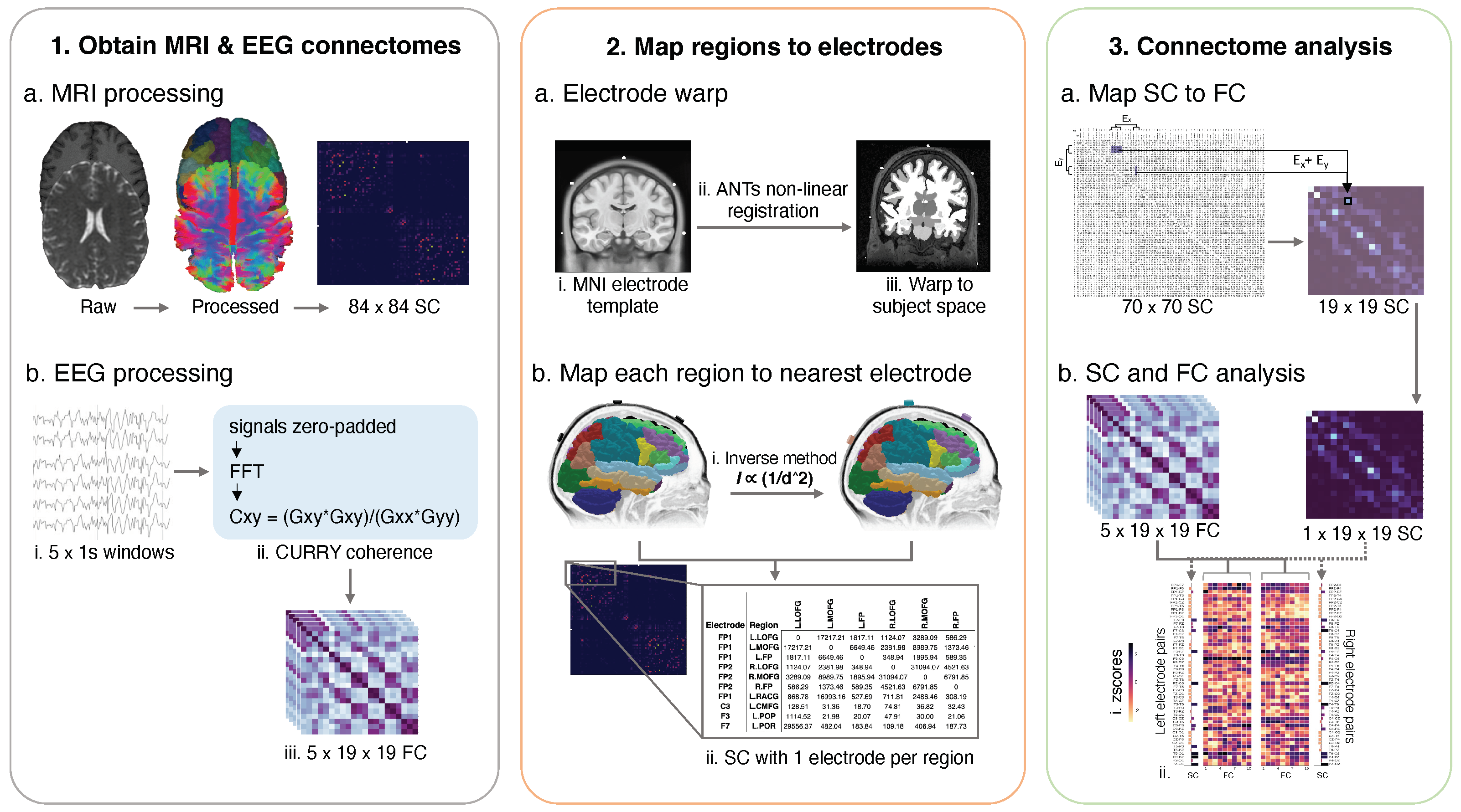
Nine adults with focal epilepsy were recruited from the Comprehensive Epilepsy Centre at the Royal Prince Alfred Hospital (RPAH, Sydney, Australia), and MRI was performed at the Brain and Mind Centre (Sydney, Australia). Inclusion criteria were adults diagnosed with focal epilepsy, aged 18–60, presenting without surgery, with a minimum of two recorded seizures, and who were willing and able to comply with the study procedures for the duration of their participation. Exclusion criteria were pregnant women and individuals with intellectual disabilities. Ethical approval was obtained from the RPAH Local Health District (RPAH-LHD) ethics committee (see Institutional Review Statement in Section 5). The entire data processing and analysis consisted of several consecutive steps, depicted in Figure 1.
2.2. Image Acquisition
Image acquisition was described previously [33]. Briefly, all scans were acquired on the same GE DiscoveryTM MR750 3T scanner (GE Medical Systems, Milwaukee, WI, USA). The following sequences were acquired for each participant: Pre-contrast 3D high-resolution T1-weighted image (0.7 mm isotropic) using fast spoiled gradient echo (SPGR) with magnetisation-prepared inversion recovery pulse (TE/TI/TR=2.8/450/7.1 ms, flip angle = 12); and axial diffusion-weighted imaging (2 mm isotropic, TE/TR = 85/8325 ms) with a uniform gradient loading (b = 1000 s/mm2) in 64 directions and 2 b0 s. An additional b0 image with reversed phase-encoding was also acquired for distortion correction [34].
2.3. Image Processing to Obtain Structural Connectomes
The T1 images were processed using a modified version of Freesurfer’s recon-all (v6.0) [35], alongside an in-house skull-stripping tool (Sydney Neuroimaging Analysis Centre). Each subject was inspected, and minor segmentation errors were manually corrected. A 5 tissue-type (5TT) image [36] was generated using MRtrix3 [37]. The T1 image was registered to the mean image; the warp was used to register the 5TT image, and the DK [32] parcellation image to the diffusion image.
Diffusion image processing was conducted using MRtrix3 [37]. The diffusion pre-processing included motion and distortion correction [34,38], bias correction using ANTs [39]. The dhollander algorithm [40] was used to estimate the response functions of the white matter, grey matter, and cerebral spinal fluid, from which constrained spherical deconvolution was used to estimate the fibre orientation distributions using MRtrix3Tissue [37]. The intensity of the white matter fibre orientation distributions was normalised [37], and used for anatomically constrained whole-brain tractography [41] (along with the registered 5TT image). The tractography specifications were as follows: 15 million tracks were generated, iFOD2 probabilistic fibre tracking [42], dynamic seeding [43], maximum length 300 mm, backtrack selected and crop at grey-matter-white-matter interface selected. For quantitative analysis, the corresponding weight for each streamline in the tractogram was derived using SIFT2 [43]. The streamlines and corresponding SIFT2 weights were used to create a weighted, undirected structural connectome (“SC”) using the registered parcellation image. All image processing steps are shown in Figure 1 (Step 1, a).
2.4. EEG Acquisition
The EEG recordings were derived from ward recordings conducted during the patients’ stay at the RPAH. The EEG was recorded using Compumedics hardware and software. The ward nurse applied the individual electrodes to the patient’s head in the standard 10/20 format using the gold standard measurement process. Once the routine clinical recording was complete, the raw EEG files were obtained, and the seizure segments annotated by the EEG technician and reviewed by a senior neurologist. All seizures were then analysed in Curry 8 (“Curry”, Compumedics Neuroscan) to obtain the functional connectomes. Curry is a neuroimaging software suite that allows the combination and analysis of multimodal data and is optimised for evaluating epilepsy-related data.
2.5. EEG Processing to Obtain Functional Connectomes
Curry was used to pre-process the EEG and obtain the sensor-based coherence matrices which represented the functional connectomes. First, we applied Curry’s automated artifact reduction and filtering tool to obtain a clean signal. Next, Curry’s coherence calculation process (shown in Figure 1, Step 1, b, ii) was used to generate coherence matrices for the first five seconds of each seizure. Specifically, using one-second non-overlapping windows starting from the annotated seizure onset time, the coherence matrices were computed from the cross-spectral densities and auto-spectral densities and of the channels x and y, using the equation
/. The resulting coherence matrices were 21 × 21; row and column headers represented single electrodes. The reference electrodes and their corresponding scores were then removed, resulting in 19 × 19 matrices, which were used as the functional connectomes (“FC”, Figure 1, Step 1, b, iii). Therefore, each electrode pair’s corresponding value was a composite of the normalised maximum similarity between the waveforms and the time-shift (delay) when the maximum similarity occurred. The electrode pair value represented the highest percentage of coherence achieved by that electrode pair in the one-second window after factoring in the signal time lag between the two electrodes.
2.6. Mapping Cortical Regions to the Nearest Electrode
This section details the processes in Step 2 of Figure 1, where we used our previously described method [30] to create a subject-specific electrode warp and map each subject’s cortical regions from the DK atlas to the nearest electrode. First, using the ANTs nonlinear registration tool, 21 electrodes in the standard MNI template space were warped to each participant’s T1 image that had been registered to the diffusion image space (Figure 1 Step 2, a, i–iii). Next, we applied our inverse square method, which incorporates the inverse square equation shown in Figure 1 (Step 2, b, i) to produce a subject-specific, one-to-one mapping of each cortical region to its nearest electrode. The inputs were each subject’s electrode warp and the cortical structure labels from Step 1. The inverse square equation holds that the light intensity of a source is inversely proportional to the square of the distance from the source. Thus, the inverse square method enabled the consideration of MRI voxel intensity in assessing the distance of each cortical region from each electrode’s centre. Voxel intensity may represent the cortex’s topological arrangement, endorsing postulation of the EEG signal strength from a given region relative to that region’s distance from the scalp. The matrix in Figure 1, (Step 2, b, ii) depicts each region with one electrode name assigned—this electrode was the closest to that region. Subcortical regions (such as the hippocampus) were not assigned electrodes as their physical distance from the scalp and positioning below other cortical regions deemed them inaccessible for accurate measurement; thus they were removed from the analysis.
2.7. Mapping the Structural Connectome to the Functional Connectome
To enable the direct, one-to-one comparison of the values in the structural and functional connectomes, the structural connectome was first condensed to match the size of the functional connectomes (from 70 × 70 to 19 × 19). Only the upper triangle of the structural connectome was used in the calculation. The output file shown in Figure 1 (Step 2, b, ii) provided the electrode names and corresponding regions (and their values) for the new structural matrix. To calculate the new value for a given electrode pair in the condensed structural connectome, the values for all regions between that given electrode pair were summed. An example is provided in Figure 1, (Step 3, a), where all values between electrodes Fz (“E”) and Fp2 (“E”) are coloured in purple. The total sum of all values between E and E was used as the new value for Fz-Fp2 (black square) in the condensed structural connectome. Once new values were computed for all electrode pairs, the diagonal line (self correlations) was removed from the structural and functional connectomes, and the connectomes were converted to a 1D array for statistical analysis.
2.8. Statistical Analysis of Structure-Function Coupling
To test whether the laterality of the strong connections matched each patient’s diagnosis, we first split the structural and functional connectomes into left and right hemispheres (Figure 1, Step 3, b) and removed cross-hemisphere electrode pairs. For example, if an electrode pair contained two electrodes in the left hemisphere (i.e., FP1-F3) or one left hemisphere and one central electrode (FP1-Fz), the electrode pair was kept. All electrode pairs that crossed from one hemisphere to the other (i.e., F3-F4) were removed. To test whether the highly connected electrode pairs from the structural and functional connectomes were congruent, we first computed the z-scores for all electrode pairs from all connectomes (Figure 1, Step 3, b, i). The z-score arrays were: a. 1 × 1D array per hemisphere for the structural connectome and b. 5 × 1D arrays (for each 1 s time window) per seizure, per hemisphere for the functional connectomes. Lastly, the structural and functional zscores from each hemisphere were displayed in parallel format for analysis (Figure 1, Step 3, b, ii).
To preserve only the most robust connections to represent high coherence between two electrodes, a z-score threshold of 2 (i.e., two standard deviations from the mean) was chosen for the structural connectome, and a threshold of 1.8 was chosen for the functional connectomes. Next, the z-scores from both connectome types were compared per one-second window from each seizure. If the same electrode pair from the structural and functional connectomes contained a z-score between 1.8 and 2 (or greater than 2), that electrode pair was classified as showing high structure-function coupling (termed “coupled electrode pairs”).
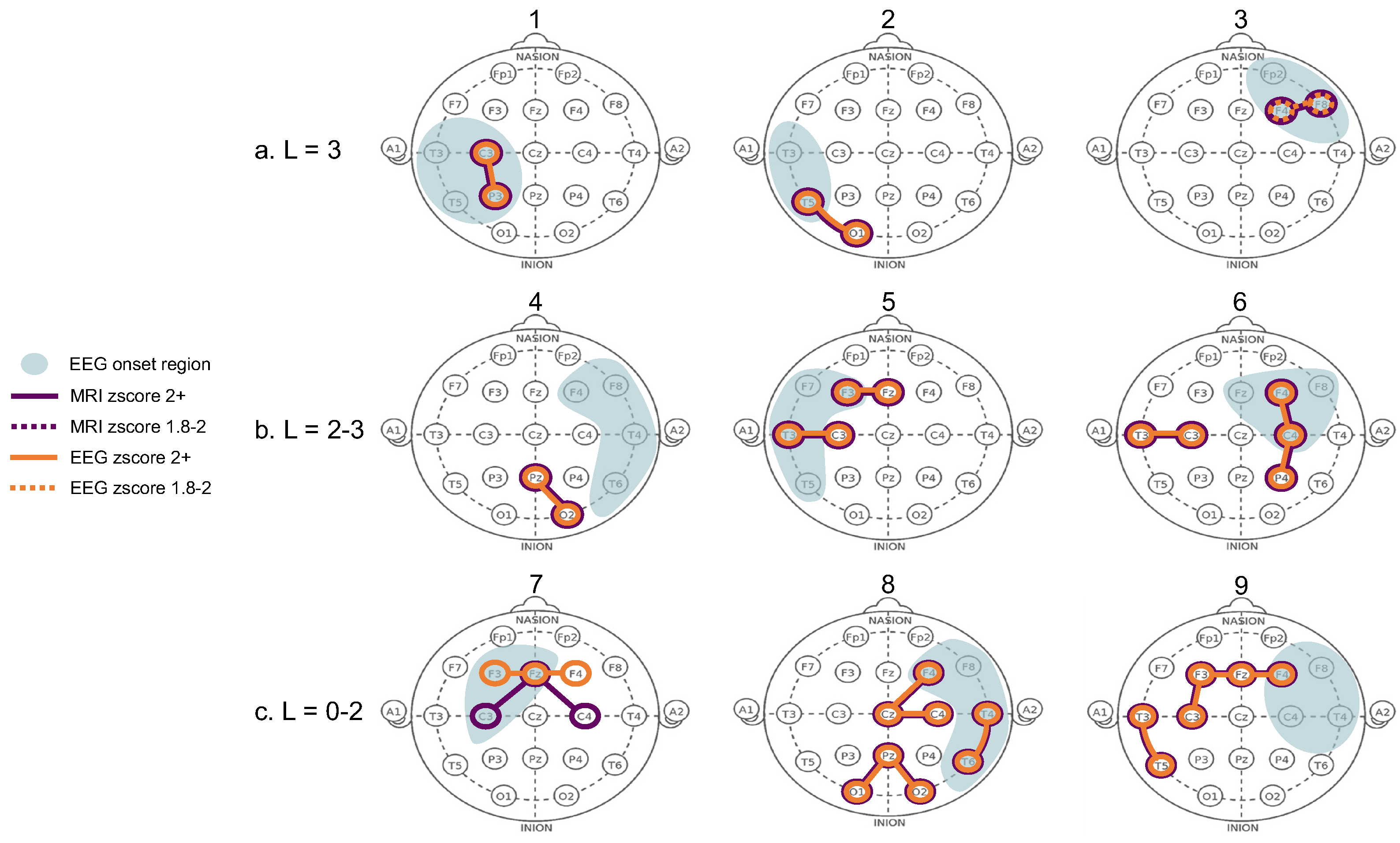
The senior neurologist provided a “laterality” score for each patient based on whether the most frequently observed seizure onset zone was consistently restricted to one hemisphere. A laterality score of zero represented poorly lateralised seizures, whilst highly lateralised seizures received a score of three. If overall, the patient had late-lateralising seizures, they were classified as being non-lateralised at onset (i.e., a score of 0–1). Each patient was also assigned an “expected onset zone”, predicated on the most frequently observed onset zone observed in all of a patient’s recorded seizures, including seizures that were poorly or non-lateralised. The neurologist reviewed the raw EEG to confirm whether the electrode pair with high structure-function coupling was congruent with the expected seizure onset zone. All z-scores and statistical analyses were produced in SPSS v28 (Armonk, NY, USA: IBM Corp).
3. Results
3.1. Demographics
Nine patients (6F, mean age 38.8 ± 11.28) were included in this study after meeting the inclusion criteria. The patient characteristics, including seizure onset zone, are shown in Table 1. Three of the nine patients presented with highly lateralised seizures; the other six had a mixture of highly lateralised and poorly lateralised seizures. All patients were diagnosed with focal epilepsy; two had experienced frequent focal to bilateral tonic-clonic (FBTC) seizures, whilst another three had infrequent FBTC seizures (experienced more than one year prior to the EEG recording).
3.2. Electrode-Region Mapping
The regions that displayed the most variance in electrode mapping across all nine patients are listed in Table 2 according to the Freesurfer region names. The majority of the variance appeared to be in the temporal regions. Manual inspection of the warped electrodes on each patient’s scalp, which were overlaid on the cortex regions, indicated that individual scalp and cortex morphology contributed to the model’s determination of the nearest electrode for a given region.
3.3. Structure-Function Coupling
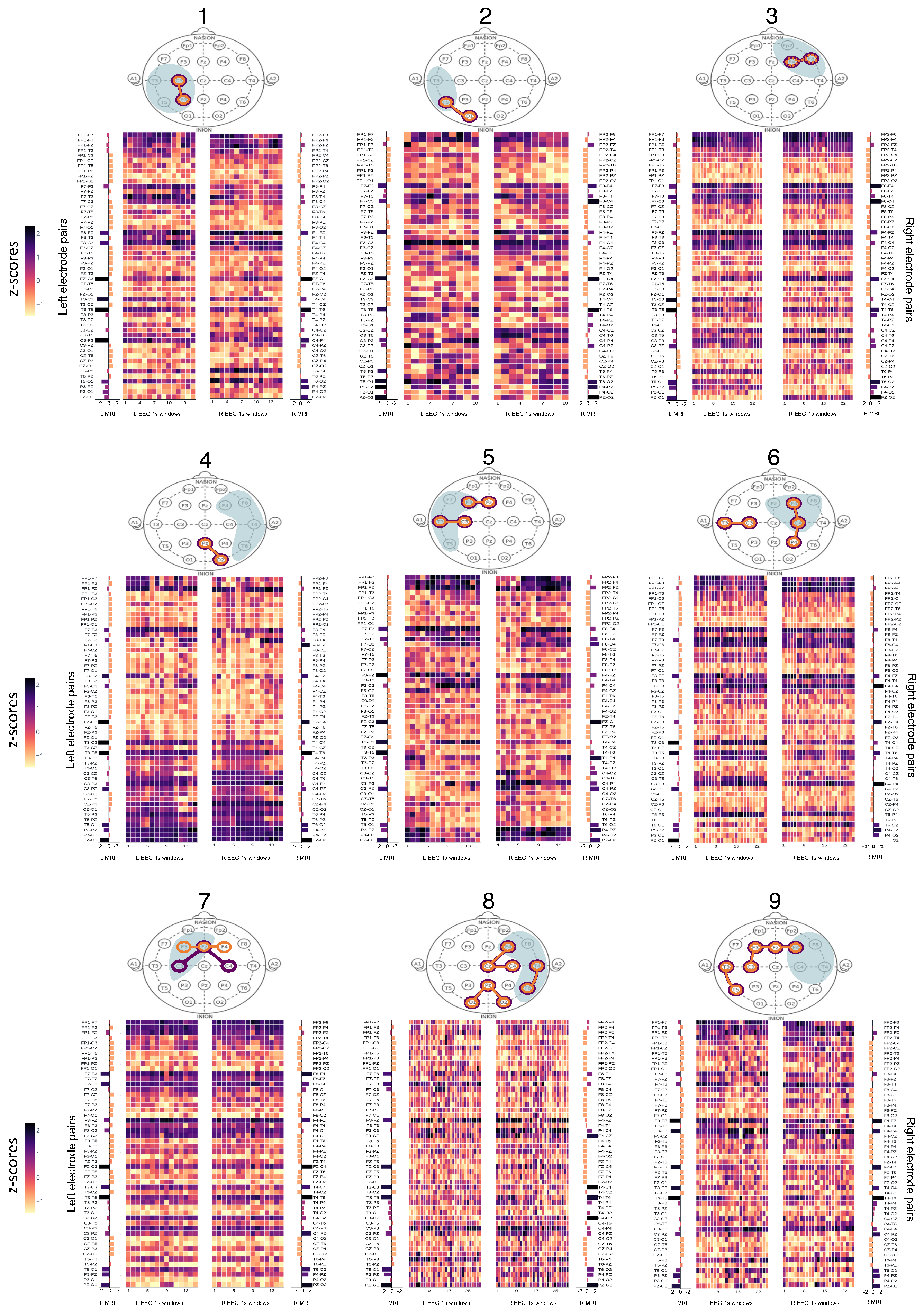
The structure-function coupling observed in the nine patients revealed three distinct groups with the following features. The first group (Patients 1–3, Figure 2a) had the highest laterality scores (L = 3), with coupled electrode pairs that consistently overlapped with the seizure onset zone. The second group (Patients 4–6, Figure 2b) had less well-lateralised seizures (L = 2–3), and the coupled electrode pairs overlapped with the onset side but not the exact zone. In Patient 4, only two out of three seizures were highly lateralised (L = 3) while the third was not (L = 2), and the electrode pair (PZ-O2) that did not overlap with the exact seizure onset zone was observed on the poorly lateralised seizure. Patient 4 also had three single electrodes from highly connected MRI and EEG pairs that overlapped inside the seizure onset zone (shown in heatmaps in Figure A1). Patients 5 and 6 were less well lateralised, and highly coupled electrode pairs were present both within and outside the seizure onset zone. In Patient 6, the electrode pair T3-C3 overlapped with the expected onset zone of the one poorly lateralised seizure. The third group (Patients 7–9, Figure 2c) were considered non-lateralised for most of their seizures. These patients generally displayed highly coupled electrode pairs that were inconsistent with the expected onset zone or had only a single overlapping MRI and EEG electrode rather than a pair (Patient 7). Figure 2 contains a condensed interpretation of the detailed results for each patient, shown in Appendix A. The overlapping electrode pairs with MRI z-scores (>2) and EEG z-scores (>1.8) are displayed. The most common seizure onset zone for each patient is also displayed.
4. Discussion
In this study, we obtained structural and functional connectomes from nine patients to investigate whether our model could uncover the structure-function coupling during seizure onset. We also examined the pattern and congruence of the structure-function coupling with the expected seizure onset zone. The first key finding was that patients with well-lateralised seizures displayed high structural-functional congruence consistent with the expected seizure onset zone. The second key finding was that patients who were not well-lateralised had varying coupled electrodes that were not consistently in the onset zone. The results indicate that for well-lateralised patients, connectivity data derived from dMRI can be a valuable tool to augment routine EEG observations. However, the dMRI should be interpreted in the context of other routinely collected data from the patient.
Our findings offer some compelling evidence for the use of dMRI in clinical practice. Firstly, in patients with high structure-function coupling in the expected onset zone, dMRI may provide additional support to the EEG observations. A recent work used intracranial EEG (iEEG) and dMRI to explore the relation between structure-function coupling and post-surgery seizure freedom [9]. The Authors showed that patients who achieved post-surgery seizure freedom had higher structure-function coupling pre-surgery. However, access to iEEG may not be feasible in the initial diagnosis stage. Additionally, the diagnostic yield of low-density scalp EEG (25 electrodes) has been suggested to be comparable to high-density EEG (256 electrodes) [44]. Taken together, our findings suggest that our model may be used during the diagnosis stage to determine the suitability of surgery for newly-diagnosed patients. Notably, we provide evidence that high structure-function coupling was present for patients regardless of whether they had previously experienced an FBTC seizure. Our finding suggests that a history of infrequent FBTC seizures (present in Patients 1 and 3) does not preclude the patient from having well-lateralised structure-function coupling.
Secondly, in the patients with poorly lateralised seizures, the structure-function coupling was more predominant in the ipsilateral hemisphere. However, the presence of structure-function coupling in the contralateral hemisphere was unsurprising, given their laterality score. In these patients, dMRI may provide additional information that can guide the placement of additional electrodes in longer ward recordings. However, a more extensive structure-function coupling model may be needed to understand whether the poor laterality can be attributed to the equally high structural connectivity in both hemispheres or some other biophysical phenomenon. Further, our model demonstrated a specific region with high structure-function coupling for Patient 8, who was initially considered poorly lateralised on EEG. Such cases highlight that dMRI may offer endorsement of a specific onset zone to support an otherwise inconclusive EEG recording.
Interestingly, the presence of high structure-function coupling in an electrode pair containing a middle electrode (FZ, CZ, PZ) was observed in several patients with a seizure laterality score of 2 or lower. For example, patients 5, 7, 8 and 9 had at least one middle electrode in the electrode pairs that showed high structure-function coupling. Their poor seizure lateralisation could be due to the electrophysiological activity beneath the middle electrode, which may drive the contralateral seizure propagation.
Given the scope of the current work, some methodological considerations may aid the interpretation of the results. Firstly, the mapping method did not appear to impact the results as well-lateralised patients had a similar number of variances in the electrode-to-region mapping as the less well-lateralised patients, for whom the structural data provided little additional information. However, laterality alone may not account for the results from patients who displayed high structure-function coupling congruent with the expected onset zone. Our selection of time window and bandwidth may have impacted the coherence score. The one-second window was perhaps not brief enough to capture the highly coherent initial EEG activity. We observed high coherence in the ipsilateral hemisphere at the 0–100 millisecond (ms) scale for some patients. The lengthy time window may have confounded this high coherence.
Further, the proposition that microscopic signal aberrations in EEG may not be observed from a macroscopically normal EEG signal is worth considering [2]. The uncertainty of empirical, visual evaluation of EEG to localise the seizure onset zone has been shown [45]. Thus, in the current work, the true onset zone for some individuals may not be observable on the raw EEG, yet may have been captured in the processed EEG coherence data. However, such postulations must be verified using high-definition EEG or intracranial/stereo EEG. Alternatively, since we combined microscopic MRI and EEG data, it is also possible that our model captured the genuine seizure onset zone. Supposing the seizure began in a different region, it could have fused in millisecond time with other active regions and thus was visually revealed in a different region on the raw EEG. Such an explanation is conceivable for individuals with FBTC or multi-onset seizures and is a topic for future investigation.
Lastly, it is feasible that the structural topology has a diminished relationship with the functional activity in some individuals. Numerous mechanisms mould the seizure propagation pathways, and within-patient variance has been shown [46]. Lateralisation may be inextricably linked to the seizure duration. However, based on our experimental design (i.e., time window selection) and modest sample size, it was not plausible to extrapolate any biophysical mechanisms that may be in force. The individuals in the third group may have less well-defined circuits, or a different epileptic pattern, i.e., multi-onset or deep structural connections or functional activity, that was not captured in the connectome reconstruction or on the scalp EEG. These concepts are the subject of ongoing work to further elaborate on this feasibility study and better explain the individual differences in the outcomes.
Although our methodology may explain some of the findings, potential limitations were inevitable. The generalisation of the results is limited by the small sample size, endorsing the need to extend this work to a larger cohort. The placement of the electrodes in the electrode warp and automated mapping cannot be deemed identical to the original, physical placement of the electrodes during the EEG recording. The electrode warp placements represented the expected actual electrode placement during the recording. This work highlights the possible variation inherent in demystifying the electrical signals captured on scalp EEG. There is an intrinsic between-patient variance in cortex and scalp morphology and thickness. The nature of the clinical procedure introduces further variance through the measurement estimation of different technicians during the application and re-application of electrodes.
The Curry sensor coherence algorithm is confined to broadband frequencies and does not compute coherence from narrow-band frequencies. Further, the Curry algorithm does not consider the spatial, topographical, morphological or biophysical implications of the scalp signal; it is calculated purely on the raw EEG wave. Therefore, our inverse square mapping method was constrained in accounting for the spatial and biophysical properties of the scalp signal measurements. It is possible that the single neurologist’s assessment of the congruency results may introduce bias. Future work will include evaluation of the EEG data by several neurologists blinded to the methodology, and an inter-rater reliability assessment (such as the Kappa statistic). Lastly, lack of control data restricts the distinction between the structure-function coupling in seizures and normal coupling in resting state or non-ictal periods.
Indeed, linking brain structure and function remains an imperfect science, confounded by individual differences in structure-function coupling [47]. Therefore extending this study to a larger cohort, with the addition of control data, is the subject of ongoing work in our lab. The inclusion of pre-ictal and cross-hemisphere connectivity data will enable further comparison and quantification of the active electrodes across varying brain states. Additionally, using coherence matrices derived from open source software could provide a point of comparison to Curry’s sensor coherence maps. Despite these restrictions, our work provides evidence that dMRI is a promising additional tool to classify patients for further investigation or surgical candidature. Our model may be practical in identifying the most active locations for sub-scalp electrodes and the patients who could benefit from ultra long-term monitoring. We show that all regions of high connectivity are not necessarily the best place for sub-scalp electrodes. We present a feasible method to distinguish patients, and patient-specific brain regions, that may be candidates for sub-scalp electrodes. With further refinement, our method could be utilised in identifying the optimal position for sub-scalp electrode placement, removing the need for more invasive EEG methods.
5. Conclusions
In conclusion, this study utilised a model to spatially map scalp electrodes to the nearest brain region and compare the structural and functional connectivity in nine patients with focal epilepsy. We showed that not all highly connected structural regions result in highly connected scalp EEG in the same region. Our findings suggest that seizures may follow strong connections intermittently and might only do so in well-lateralised patients and not for every seizure. Less well-lateralised patients displayed some high structure-function coupling in the ipsilateral hemisphere, but this was inconsistent. Our findings contribute to the evidence supporting the use of dMRI in clinical practice, which can guide patient-specific electrode placement and enhance the detection of the seizure onset zone. Future work will include comparisons with open source software and the addition of interictal and control data.
Author Contributions
Conceptualisation, C.M., C.W. and A.N.; methodology, C.M., C.W. and A.N.; clinical data acquisition, C.M. and A.N.; data curation, C.M. and A.D.; diffusion imaging pipeline, implementation and analysis, C.M., A.D. and C.W.; statistical analysis, C.M. and C.W.; manuscript writing, C.M.; manuscript revision and editing C.M., A.D., M.B., O.K., C.W. and A.N.; clinical advisory and results interpretation, A.N. All authors have read and agreed to the published version of the manuscript.
Funding
This research received no specific external funding.
Institutional Review Board Statement
All research and methods were performed in accordance with the Declaration of Helsinki, and the relevant guidelines and regulations prescribed by the RPAH-LHD and ethics committees. The study was approved by the Ethics Committee from the RPAH Local Health District (RPAH-LHD). The protocol number and ethics approval ID for the MRI data are X14-0347 and HREC/14/RPAH/467. The protocol number and ethics approval ID for the EEG data are X19-0323 and 2019/ETH11868.
Informed Consent Statement
The requirement for informed consent was waived in the approved ethics for the EEG data (protocol number and approval ID are X19-0323 and 2019/ETH11868) since only de-identified EEG data was acquired. Written informed consent was obtained from all participants who attended the Brain and Mind Centre for an MRI scan, as per the approved MRI ethics (protocol number and approval ID are X14-0347 and HREC/14/RPAH/467).
Data Availability Statement
The datasets generated and/or analysed during the current study are not publicly available because they are RPAH patients and can only be accessed by authorised individuals named on the approved ethics. However, de-identified, processed data can be made available upon request to the corresponding author, and subject to approval from the governing ethics entities at the RPAH and The University of Sydney.
Acknowledgments
The Authors acknowledge all staff at the Comprehensive Epilepsy Centre at the RPAH, particularly Maricar Senturias (RN/ACNC Epilepsy), who assisted with patient recruitment. The Authors acknowledge the radiology staff at i-MED Radiology for their assistance in obtaining the MRI data. The Authors acknowledge the research funding support from UCB Australia Pty Ltd. C.M. acknowledges scholarship support from the Nerve Research Foundation, University of Sydney. A.D. acknowledges funding from St. Vincent’s Hospital. O.K. acknowledges the partial support provided by The University of Sydney through a SOAR Fellowship and Microsoft’s partial support through a Microsoft AI for Accessibility grant. CW acknowledges research funding from the Nerve Research Foundation, University of Sydney.
Conflicts of Interest
The Authors declare no conflict of interest. The funders had no role in the design of the study; in the collection, analyses, or interpretation of data; in the writing of the manuscript; or in the decision to publish the results.
Appendix A
Figure A1.
Heatmaps of z-scores from MRI and EEG connectomes. L: Left, R: Right. Patients are numbered 1–9 above each “head” and their respective connectomes are shown below the “head” map in the same grouping as Figure 2 in the main text. The “EEG 1s windows” depict the left and right side of each EEG connectome, split into 1 s windows. The structural (MRI) connectomes are split into left and right sides (“L MRI” and “R MRI”) and positioned alongside the matching EEG connectome side (i.e., left MRI next to left EEG connectome). The left and right electrode pairs are listed next to the respective side of the connectome.

References
- Weng, Y.; Larivière, S.; Caciagli, L.; Vos de Wael, R.; Rodríguez-Cruces, R.; Royer, J.; Xu, Q.; Bernasconi, N.; Bernasconi, A.; Thomas Yeo, B.; et al. Macroscale and microcircuit dissociation of focal and generalized human epilepsies. Commun. Biol. 2020, 3, 1–11. [Google Scholar] [CrossRef] [PubMed]
- Zijlmans, M.; Zweiphenning, W.; van Klink, N. Changing concepts in presurgical assessment for epilepsy surgery. Nat. Rev. Neurol. 2019, 15, 594–606. [Google Scholar] [CrossRef] [PubMed]
- Babaeeghazvini, P.; Rueda-Delgado, L.M.; Gooijers, J.; Swinnen, S.P.; Daffertshofer, A. Brain Structural and Functional Connectivity: A Review of Combined Works of Diffusion Magnetic Resonance Imaging and Electro-Encephalography. Front. Hum. Neurosci. 2021, 15, 585. [Google Scholar] [CrossRef] [PubMed]
- Friston, K.J. Functional and effective connectivity in neuroimaging: A synthesis. Hum. Brain Mapp. 1994, 2, 56–78. [Google Scholar] [CrossRef]
- Honey, C.J.; Sporns, O.; Cammoun, L.; Gigandet, X.; Thiran, J.P.; Meuli, R.; Hagmann, P. Predicting human resting-state functional connectivity from structural connectivity. Proc. Natl. Acad. Sci. USA 2009, 106, 2035–2040. [Google Scholar] [CrossRef] [PubMed] [Green Version]
- Shah, P.; Ashourvan, A.; Mikhail, F.; Pines, A.; Kini, L.; Oechsel, K.; Das, S.R.; Stein, J.M.; Shinohara, R.T.; Bassett, D.S.; et al. Characterizing the role of the structural connectome in seizure dynamics. Brain 2019, 142, 1955–1972. [Google Scholar] [CrossRef]
- Vattikonda, A.N.; Hashemi, M.; Sip, V.; Woodman, M.M.; Bartolomei, F.; Jirsa, V.K. Identifying spatio-temporal seizure propagation patterns in epilepsy using Bayesian inference. Commun. Biol. 2021, 4, 1–13. [Google Scholar] [CrossRef] [PubMed]
- Lascano, A.M.; Perneger, T.; Vulliemoz, S.; Spinelli, L.; Garibotto, V.; Korff, C.M.; Vargas, M.I.; Michel, C.M.; Seeck, M. Yield of MRI, high-density electric source imaging (HD-ESI), SPECT and PET in epilepsy surgery candidates. Clin. Neurophysiol. 2016, 127, 150–155. [Google Scholar] [CrossRef] [PubMed] [Green Version]
- Sinha, N.; Duncan, J.S.; Diehl, B.; Chowdhury, F.A.; de Tisi, J.; Miserocchi, A.; McEvoy, A.W.; Davis, K.A.; Vos, S.B.; Winston, G.P.; et al. Intracranial EEG structure-function coupling predicts surgical outcomes in focal epilepsy. arXiv 2022, arXiv:2204.08086. [Google Scholar] [CrossRef]
- Chiang, S.; Stern, J.M.; Engel, J., Jr.; Haneef, Z. Structural–functional coupling changes in temporal lobe epilepsy. Brain Res. 2015, 1616, 45–57. [Google Scholar] [CrossRef]
- O’Muircheartaigh, J.; Keller, S.S.; Barker, G.J.; Richardson, M.P. White matter connectivity of the thalamus delineates the functional architecture of competing thalamocortical systems. Cereb. Cortex 2015, 25, 4477–4489. [Google Scholar] [CrossRef] [PubMed] [Green Version]
- Morgan, V.L.; Sainburg, L.E.; Johnson, G.W.; Janson, A.; Levine, K.K.; Rogers, B.P.; Chang, C.; Englot, D.J. Presurgical temporal lobe epilepsy connectome fingerprint for seizure outcome prediction. Brain Commun. 2022, 4, fcac128. [Google Scholar] [CrossRef] [PubMed]
- Gong, J.; Luo, C.; Chang, X.; Zhang, R.; Klugah-Brown, B.; Guo, L.; Xu, P.; Yao, D. White matter connectivity pattern associate with characteristics of scalp EEG signals. Brain Topogr. 2017, 30, 797–809. [Google Scholar] [CrossRef] [PubMed]
- Deslauriers-Gauthier, S.; Lina, J.M.; Butler, R.; Whittingstall, K.; Gilbert, G.; Bernier, P.M.; Deriche, R.; Descoteaux, M. White matter information flow mapping from diffusion MRI and EEG. NeuroImage 2019, 201, 116017. [Google Scholar] [CrossRef] [Green Version]
- Sadaghiani, S.; Brookes, M.J.; Baillet, S. Connectomics of human electrophysiology. NeuroImage 2022, 247, 118788. [Google Scholar] [CrossRef] [PubMed]
- Lagarde, S.; Buzori, S.; Trebuchon, A.; Carron, R.; Scavarda, D.; Milh, M.; McGonigal, A.; Bartolomei, F. The repertoire of seizure onset patterns in human focal epilepsies: Determinants and prognostic values. Epilepsia 2019, 60, 85–95. [Google Scholar] [CrossRef] [PubMed] [Green Version]
- Fitzgerald, Z.; Morita-Sherman, M.; Hogue, O.; Joseph, B.; Alvim, M.K.; Yasuda, C.L.; Vegh, D.; Nair, D.; Burgess, R.; Bingaman, W.; et al. Improving the prediction of epilepsy surgery outcomes using basic scalp EEG findings. Epilepsia 2021, 62, 2439–2450. [Google Scholar] [CrossRef] [PubMed]
- Chu, C.J.; Tanaka, N.; Diaz, J.; Edlow, B.L.; Wu, O.; Hämäläinen, M.; Stufflebeam, S.; Cash, S.S.; Kramer, M.A. EEG functional connectivity is partially predicted by underlying white matter connectivity. Neuroimage 2015, 108, 23–33. [Google Scholar] [CrossRef] [PubMed] [Green Version]
- Cserpan, D.; Gennari, A.; Gaito, L.; Lo Biundo, S.P.; Tuura, R.; Sarnthein, J.; Ramantani, G. Scalp HFO rates are higher for larger lesions. Epilepsia Open 2022, 7, 496–503. [Google Scholar] [CrossRef]
- Samadzadehaghdam, N.; Makkiabadi, B.; Masjoodi, S.; Mohammadi, M.; Mohagheghian, F. A new linearly constrained minimum variance beamformer for reconstructing EEG sparse sources. Int. J. Imaging Syst. Technol. 2019, 29, 686–700. [Google Scholar] [CrossRef]
- Rubega, M.; Carboni, M.; Seeber, M.; Pascucci, D.; Tourbier, S.; Toscano, G.; Van Mierlo, P.; Hagmann, P.; Plomp, G.; Vulliemoz, S.; et al. Estimating EEG source dipole orientation based on singular-value decomposition for connectivity analysis. Brain Topogr. 2019, 32, 704–719. [Google Scholar] [CrossRef] [PubMed] [Green Version]
- Neugebauer, F.; Antonakakis, M.; Unnwongse, K.; Parpaley, Y.; Wellmer, J.; Rampp, S.; Wolters, C.H. Validating EEG, MEG and combined MEG and EEG beamforming for an estimation of the epileptogenic zone in focal cortical dysplasia. Brain Sci. 2022, 12, 114. [Google Scholar] [CrossRef] [PubMed]
- Zagorchev, L.; Brueck, M.; Fläschner, N.; Wenzel, F.; Hyde, D.; Ewald, A.; Peters, J. Patient-specific sensor registration for electrical source imaging using a deformable head model. IEEE Trans. Biomed. Eng. 2020, 68, 267–275. [Google Scholar] [CrossRef] [PubMed]
- Proix, T.; Bartolomei, F.; Guye, M.; Jirsa, V.K. Individual brain structure and modelling predict seizure propagation. Brain 2017, 140, 641–654. [Google Scholar] [CrossRef] [PubMed] [Green Version]
- Jirsa, V.K.; Proix, T.; Perdikis, D.; Woodman, M.M.; Wang, H.; Gonzalez-Martinez, J.; Bernard, C.; Bénar, C.; Guye, M.; Chauvel, P.; et al. The virtual epileptic patient: Individualized whole-brain models of epilepsy spread. Neuroimage 2017, 145, 377–388. [Google Scholar] [CrossRef] [PubMed]
- Varatharajah, Y.; Berry, B.; Joseph, B.; Balzekas, I.; Pal Attia, T.; Kremen, V.; Brinkmann, B.; Iyer, R.; Worrell, G. Characterizing the electrophysiological abnormalities in visually reviewed normal EEGs of drug-resistant focal epilepsy patients. Brain Commun. 2021, 3, fcab102. [Google Scholar] [CrossRef] [PubMed]
- Asadzadeh, S.; Rezaii, T.Y.; Beheshti, S.; Delpak, A.; Meshgini, S. A systematic review of EEG source localization techniques and their applications on diagnosis of brain abnormalities. J. Neurosci. Methods 2020, 339, 108740. [Google Scholar] [CrossRef] [PubMed]
- Sharma, P.; Seeck, M.; Beniczky, S. Accuracy of interictal and ictal electric and magnetic source imaging: A systematic review and meta-analysis. Front. Neurol. 2019, 10, 1250. [Google Scholar] [CrossRef] [Green Version]
- Birot, G.; Spinelli, L.; Vulliémoz, S.; Mégevand, P.; Brunet, D.; Seeck, M.; Michel, C.M. Head model and electrical source imaging: A study of 38 epileptic patients. NeuroImage Clin. 2014, 5, 77–83. [Google Scholar] [CrossRef]
- Maher, C.; D’Souza, A.; Zeng, R.; Wang, D.; Barnett, M.; Kavehei, O.; Armin, N.; Wang, C. Automated method to map cortical brain regions to the nearest scalp electroencephalography electrode. Epilepsia 2021, 62, 238–239. [Google Scholar]
- Rados, M.; Mouthaan, B.; Barsi, P.; Carmichael, D.; Heckemann, R.A.; Kelemen, A.; Kobulashvili, T.; Kuchukhidze, G.; Marusic, P.; Minkin, K.; et al. Diagnostic value of MRI in the presurgical evaluation of patients with epilepsy: Influence of field strength and sequence selection: A systematic review and meta-analysis from the E-PILEPSY Consortium. Epileptic Disord. 2022, 24, 323–342. [Google Scholar] [CrossRef] [PubMed]
- Desikan, R.S.; Ségonne, F.; Fischl, B.; Quinn, B.T.; Dickerson, B.C.; Blacker,, D.; Buckner, R.L.; Dale, A.M.; Maguire, R.P.; Hyman, B.T.; et al. An automated labeling system for subdividing the human cerebral cortex on MRI scans into gyral based regions of interest. NeuroImage 2006, 31, 968–980. [Google Scholar] [CrossRef] [PubMed]
- Maher, C.; D’Souza, A.; Zeng, R.; Barnett, M.; Kavehei, O.F.; Nikpour, A.; Wang, C. White matter alterations in focal to bilateral tonic-clonic seizures. Front. Neurol. 2022, 13, 972590. [Google Scholar] [CrossRef]
- Andersson, J.L.; Sotiropoulos, S.N. An integrated approach to correction for off-resonance effects and subject movement in diffusion MR imaging. NeuroImage 2016, 125, 1063–1078. [Google Scholar] [CrossRef] [Green Version]
- Fischl, B. Freesurfer. Neuroimage 2012, 62, 774–781. [Google Scholar] [CrossRef] [Green Version]
- Smith, R.; Skoch, A.; Bajada, C.J.; Caspers, S.; Connelly, A. Hybrid surface-volume segmentation for improved anatomically-constrained tractography. In Proceedings of the OHBM Annual Meeting, Virtual, 23 June–3 July 2020; pp. 1–5. [Google Scholar]
- Tournier, J.D.; Smith, R.; Raffelt, D.; Tabbara, R.; Dhollander, T.; Pietsch, M.; Christiaens, D.; Jeurissen, B.; Yeh, C.H.; Connelly, A. MRtrix3: A fast, flexible and open software framework for medical image processing and visualisation. NeuroImage 2019, 202, 116137. [Google Scholar] [CrossRef] [PubMed]
- Smith, S.M.; Jenkinson, M.; Woolrich, M.W.; Beckmann, C.F.; Behrens, T.E.; Johansen-Berg, H.; Bannister, P.R.; De Luca, M.; Drobnjak, I.; Flitney, D.E.; et al. Advances in functional and structural MR image analysis and implementation as FSL. NeuroImage 2004, 23, S208–S219. [Google Scholar] [CrossRef] [PubMed] [Green Version]
- Tustison, N.J.; Avants, B.B.; Cook, P.A.; Zheng, Y.; Egan, A.; Yushkevich, P.A.; Gee, J.C. N4ITK: Improved N3 bias correction. IEEE Trans. Med. Imaging 2010, 29, 1310–1320. [Google Scholar] [CrossRef] [Green Version]
- Dhollander, T.; Raffelt, D.; Connelly, A. Unsupervised 3-tissue response function estimation from single-shell or multi-shell diffusion MR data without a co-registered T1 image. In Proceedings of the ISMRM Workshop on Breaking the Barriers of Diffusion MRI. ISMRM, Lisbon, Portugal, 12–16 September 2016; Volume 5. [Google Scholar]
- Smith, R.E.; Tournier, J.D.; Calamante, F.; Connelly, A. Anatomically-constrained tractography: Improved diffusion MRI streamlines tractography through effective use of anatomical information. NeuroImage 2012, 62, 1924–1938. [Google Scholar] [CrossRef]
- Tournier, J.D.; Calamante, F.; Connelly, A. Improved probabilistic streamlines tractography by 2nd order integration over fibre orientation distributions. In Proceedings of the International Society for Magnetic Resonance in Medicine, Stockholm, Sweden, 1–7 May 2010; p. 1670. [Google Scholar]
- Smith, R.E.; Tournier, J.D.; Calamante, F.; Connelly, A. SIFT2: Enabling dense quantitative assessment of brain white matter connectivity using streamlines tractography. NeuroImage 2015, 119, 338–351. [Google Scholar] [CrossRef]
- Justesen, A.B.; Foged, M.T.; Fabricius, M.; Skaarup, C.; Hamrouni, N.; Martens, T.; Paulson, O.B.; Pinborg, L.H.; Beniczky, S. Diagnostic yield of high-density versus low-density eeg: The effect of spatial sampling, timing and duration of recording. Clin. Neurophysiol. 2019, 130, 2060–2064. [Google Scholar] [CrossRef] [PubMed]
- Davis, K.A.; Devries, S.P.; Krieger, A.; Mihaylova, T.; Minecan, D.; Litt, B.; Wagenaar, J.B.; Stacey, W.C. The effect of increased intracranial EEG sampling rates in clinical practice. Clin. Neurophysiol. 2018, 129, 360–367. [Google Scholar] [CrossRef] [PubMed]
- Schroeder, G.M.; Chowdhury, F.A.; Cook, M.J.; Diehl, B.; Duncan, J.S.; Karoly, P.J.; Taylor, P.N.; Wang, Y. Multiple mechanisms shape the relationship between pathway and duration of focal seizures. Brain Commun. 2022, 4, fcac173. [Google Scholar] [CrossRef] [PubMed]
- Suárez, L.E.; Markello, R.D.; Betzel, R.F.; Misic, B. Linking structure and function in macroscale brain networks. Trends Cogn. Sci. 2020, 24, 302–315. [Google Scholar] [CrossRef]
Figure 1.
Schematic of data processing and analysis steps. To obtain the structural connectomes (“SC”, Step 1, a), the dMRI was processed, and anatomically-constrained probabilistic tractography was conducted as outlined in Section 2.3. Cortical regions of interest were based on the Desikan-Killiany (DK) [32] atlas. To obtain the functional connectomes (“FC”), the first 5 s of a given seizure were selected using one-second windows. Each one-second window was processed using Curry’s sensor coherence algorithm (Step 1, b, ii), producing a 21 × 21 coherence matrix. The reference electrodes were removed before statistical analysis, resulting in a 19 × 19 coherence matrix which was used as the functional connectome. In Step 2, the ANTs non-linear registration tool was used to warp electrodes in the MNI template space to the subject space, creating a subject-specific electrode warp (a, i–iii). To produce a subject-specific, one-to-one map of each cortical region to its nearest electrode, we applied our inverse square method (b, i). The inputs were each subject’s electrode warp and cortical region labels from Step 1. The result was a structural connectome with an electrode name corresponding to each of the 70 regions, i.e., F7/L.LOFG (b, ii). In Step 3 (a), the 70 × 70 structural connectome was condensed to match the dimensions of the functional matrix (19 × 19). Specifically, the values of all regions corresponding to a given electrode pair were summed, and the total value was used as the connectivity value for that same electrode pair in the new condensed structural connectome. Lastly, z-scores were computed for all connectivity values in the structural and functional connectomes (b, i,ii) and the statistical analysis was conducted.

Figure 2.
Highly connected electrode pairs in structural and functional connectome. Each “head” shows a schematic of the electrode pairs for each of the nine patients (numbered 1–9 above each head). The “L” value represents each patient’s overall seizure lateralisation score based on their available recorded seizures. A score of zero represented poorly lateralised seizures, whilst highly lateralised seizures received a score of three. The patients’ seizures stratified them into three categories: patients 1–3 had high laterality, patients 4–6 had some seizures that were well lateralised, while others were not, and patients 7–9 had poor laterality in all seizures. The purple lines (and circled electrodes) represent the electrode pairs that displayed strong connectivity (z-scores > 2) in the structural (MRI) connectome. The orange lines (and circled electrodes) represent the electrode pairs that displayed strong connectivity (z-scores > 2) in the functional (EEG) connectome. Dotted lines in either colour represent a z-score of 1.8–2. The blue shading represents the most frequently observed seizure onset zone for a given patient, as observed from their ward EEG recordings. If a seizure did not have a specific onset region within the first 5 s, it was considered non-lateralised, even if it displayed late-lateralisation. Purple and orange circled electrodes in the blue shaded areas represent high structure-function coupling in the seizure onset zone.


Table 1.
Characteristics of patients.
| Patient | Sex | Classification | MRI Diagnosis | Onset Age | Age at MRI | Duration | Drug Res. | Handedness |
|---|---|---|---|---|---|---|---|---|
| 1 | F | Left fronto-temporal | Normal | 49 | 53 | 4 | Y | R |
| 2 | M | Left fronto-temporal | HS | 21 | 49 | 28 | Y | L |
| 3 | F | Right frontal | Normal | 38 | 48 | 10 | N | R |
| 4 | F | Right temporal | Normal | 16 | 29 | 13 | Y | U |
| 5 | M | Left fronto-temporal | Normal | 16 | 31 | 15 | Y | R |
| 6 | F | Left occipital | Normal | 12 | 47 | 35 | Y | R |
| 7 | F | Left fronto-temporal | Normal | 35 | 48 | 13 | N | R |
| 8 | M | Right fronto-temporal | Normal | 15 | 33 | 18 | Y | R |
| 9 | M | Right temporal | Normal | 22 | 29 | 7 | Y | R |
Key: L: left, R: right, U: unknown; † HS: hippocampal sclerosis; ‡ slight enlargement of right amygdala.
Table 2.
Between patient region variance in the region to electrode mapping.
| Subject No. | 1 | 2 | 3 | 4 | 5 | 6 | 7 | 8 | 9 |
|---|---|---|---|---|---|---|---|---|---|
| Region Name | |||||||||
| L. rostralanteriorcingulate | FP1 | FP1 | FP1 | FZ | F3 | FP1 | FZ | FP1 | FP1 |
| R. rostralanteriorcingulate | FP2 | FP2 | FP2 | FZ | FP2 | FP2 | FZ | F4 | FP2 |
| L. parsopercularis | F3 | F7 | F7 | F3 | F7 | F7 | T3 | F7 | F3 |
| R. parsopercularis | F8 | F8 | F8 | F8 | F8 | F8 | F4 | T4 | F4 |
| L. insula | T3 | F7 | T3 | F7 | T3 | T3 | T3 | T3 | T3 |
| R. insula | T4 | F8 | F8 | F8 | F8 | T4 | C4 | T4 | T4 |
| L. inferiortemporal | T5 | T5 | T5 | T5 | T3 | T5 | T5 | T3 | T5 |
| R. inferiortemporal | T6 | T4 | T6 | T6 | T4 | T6 | T6 | T4 | T6 |
| L. lateralorbitofrontal | FP1 | F7 | F7 | F7 | F7 | F7 | F7 | F7 | F7 |
| R. lateralorbitofrontal | FP2 | F8 | F8 | F8 | F8 | F8 | F4 | F8 | FP2 |
| L. cuneus | O1 | O1 | O1 | O1 | O1 | O1 | PZ | O1 | O1 |
| R. cuneus | O2 | O2 | O2 | PZ | O2 | O2 | PZ | O2 | O2 |
| L. transversetemporal | T3 | T3 | T3 | C3 | T3 | T3 | T3 | T3 | T3 |
| R. transversetemporal | T4 | T4 | T4 | C4 | T4 | T4 | T4 | T4 | T4 |
| L. caudalanteriorcingulate | FZ | FZ | FZ | FZ | F3 | FZ | FZ | F3 | FZ |
| R. caudalanteriorcingulate | FZ | FZ | FZ | FZ | FZ | FZ | FZ | F4 | FZ |
| L. isthmuscingulate | PZ | PZ | PZ | CZ | PZ | PZ | PZ | PZ | PZ |
| R. isthmuscingulate | PZ | PZ | PZ | CZ | PZ | PZ | PZ | PZ | PZ |
| R. bankssts | T6 | T6 | T4 | T6 | T4 | T6 | T6 | T6 | T6 |
| R. superiorfrontal | FZ | FZ | FZ | FZ | FZ | FZ | FZ | CZ | FZ |
| R. caudalmiddlefrontal | C4 | C4 | C4 | F4 | C4 | C4 | C4 | C4 | C4 |
| R. temporalpole | F8 | F8 | F8 | F8 | F8 | F8 | F8 | T4 | F8 |
| L. supramarginal | C3 | P3 | C3 | C3 | C3 | C3 | C3 | C3 | C3 |
| L. superiorparietal | P3 | PZ | PZ | PZ | PZ | PZ | PZ | PZ | PZ |
Key: L: left, R: right, bankssts: banks of the superior temporal sulcus.
Publisher’s Note: MDPI stays neutral with regard to jurisdictional claims in published maps and institutional affiliations. |
© 2022 by the authors. Licensee MDPI, Basel, Switzerland. This article is an open access article distributed under the terms and conditions of the Creative Commons Attribution (CC BY) license (https://creativecommons.org/licenses/by/4.0/).
Share and Cite
MDPI and ACS Style
Maher, C.; D’Souza, A.; Barnett, M.; Kavehei, O.; Wang, C.; Nikpour, A. Structure-Function Coupling Reveals Seizure Onset Connectivity Patterns. Appl. Sci. 2022, 12, 10487. https://0-doi-org.brum.beds.ac.uk/10.3390/app122010487
AMA Style
Maher C, D’Souza A, Barnett M, Kavehei O, Wang C, Nikpour A. Structure-Function Coupling Reveals Seizure Onset Connectivity Patterns. Applied Sciences. 2022; 12(20):10487. https://0-doi-org.brum.beds.ac.uk/10.3390/app122010487
Chicago/Turabian StyleMaher, Christina, Arkiev D’Souza, Michael Barnett, Omid Kavehei, Chenyu Wang, and Armin Nikpour. 2022. "Structure-Function Coupling Reveals Seizure Onset Connectivity Patterns" Applied Sciences 12, no. 20: 10487. https://0-doi-org.brum.beds.ac.uk/10.3390/app122010487
Note that from the first issue of 2016, this journal uses article numbers instead of page numbers. See further details here.