
Road Extraction Based on Improved Convolutional Neural Networks with Satellite Images

1
School of Software Engineering, Chengdu University of Information Technology, Chengdu 610225, China
2
Sichuan Province Engineering Technology Research Center of Support Software of Informatization Application, Chengdu 610225, China
3
School of Automation, University of Electronic Science and Technology of China, Chengdu 610054, China
*
Authors to whom correspondence should be addressed.
Appl. Sci. 2022, 12(21), 10800; https://0-doi-org.brum.beds.ac.uk/10.3390/app122110800
Submission received: 30 September 2022
/
Revised: 15 October 2022
/
Accepted: 19 October 2022
/
Published: 25 October 2022
(This article belongs to the Special Issue Advances in Artificial Intelligence for Perception Augmentation and Reasoning)
Abstract
:Deep learning has been applied in various fields for its effective and accurate feature learning capabilities in recent years. Currently, information extracted from remote sensing images with the learning methods has become the most relevant research area for its developed precision. In terms of developing segmentation precision and reducing calculation power consumption, the improved deep learning methods have received more attention, and the improvement of semantic segmentation architectures has been a popular solution. This research presents a learning method named D-DenseNet with a new structure for road extraction. The methods for the improvement are divided into two stages: (1) alternate the consecutive dilated convolutions number in the structure of the network (2) the stem block is arranged as the initial block. So, dilated convolution can obtain more global context information through the whole network. Further, the D-DenseNet restructures D-LinkNet by taking DenseNet as its backbone instead of ResNet, which can expand the receptive field and accept more feature information. The D-DenseNet is effective because of its 119 M model size and 57.96% IoU on the processing test data and 99.3 M modes size and 66.26% on the public dataset, which achieved the research objective for reducing model size and developing segmentation precision—IoU. The experiment indicates that the D-Dense block and the stem block are effective for developing road extraction, and the appropriate number of convolution layers is also essential for model evaluation.
1. Introduction
Recently, deep learning technology has been popular for its significant effects on the image field, such as image classification [1], information extraction [2], prediction [3] and semantic segmentation [4]. Convolutional neural networks (CNNs) are accepted as the most effective method for image processing, and adaptations of convolutional networks have been used to solve semantic segmentation problems. Image classification is a relatively easy task in computer vision, because it only needs to classify one image that contains one target object into the given set of categories, while prediction is difficult, because it needs to focus on pixel-level and contextual reasoning [5]. Many application areas adopted these CNNs, since they have better accuracy and efficiency. Convolutional kernel size is closely related to the receptive field, a key parameter for semantic segmentation accuracy. In terms of the kernel size problem, dilated convolution was proposed for expanding the receptive field [6], which is suitable for dense prediction without a reduction in resolution, coverage and parameters. D-LinkNet [7] is a popular method, and its backbone is based on LinkNet with ResNet [8], which can match the image processing requirements without losing the image pixel contents. Further, many networks were proposed based on D-LinkNet that can obtain better accuracy for information extraction from various kinds of images, and deeper CNNs are more effective for some special image tasks.
Generally, more attention has been given to the structure of CNNs, and layers are added for network efficiency. Farabet et al. proposed a Laplacian pyramid for transforming the input images [9]. Pinheiro et al. presented a coarse-to-fine method to process multi-scale inputting images [10]. Further, an encoder–decoder structure was popular for its effectiveness, and many networks preferred to adopt such multi-scale context processing [11,12,13]. In addition, some networks for semantic segmentation showed effectiveness with a similar structure to that of the encoder–decoder structure [14]. The structure of CNNs has been adjusted in various methods and has become an effective way to improve the corresponding networks.
Many networks were improved by adjusting various enlarging rates of various kernel sizes. In addition, different structures of images can be plugged into the mode [15]. Consequently, an improved method was proposed by adjusting the kernel size with multiscale context aggregation to develop the road extraction precision [16].
Low-level road extraction from satellite images presents many difficult tasks for mapping complex scenes in the remote sensing field. For instance, roads are always narrow and only occupy a tiny part of the whole image, so capturing this global feature is a difficult job. Further, different kinds of roads have different surface features, such as diverse roads, expressways, urban roads, mountain roads, and country roads. In addition, road areas are covered with trees, cars and shadows in satellite images. The above factors make automated extraction of roads from satellite images a difficult task. Many researchers had applied deep learning method to information extraction with the remote sensing images, and proposed effective results [17,18,19]. Further, classification has been given more attention in the deep learning field [20,21]. Obviously, road extraction can be taken as a classification problem, and each pixel is distinguished as in or out of a road [7]. In this research, an improved network has been proposed combining dilated convolution layers and previous layers in a building block, and D-LinkNet and the D-Dense block are also introduced in networks for low-level road extraction. Meanwhile, the advantage of dilated convolution and the D-Dense block can come with challenges. Further, the presented network has been tested through controlled experiments with the research dataset and the public dataset. The experiments show that the improved networks with the D-Dense block can develop pixel-level accuracy for semantic segmentation, and model size and IoU are better than that of other models after comparison.
2. Methods
From Section 1, network construction for semantic segmentations involves four basic parts—the encoder, the decoder, the center part and the skip connection. First, the encoder inputs images and extracts feature by stacking convolutional and pooling layers. Second, the decoder restores the detailed features and expands feature maps with deconvolutional layers. Third, the center part can be taken as a model for expanding the receptive field, creating ensembles of features and obtaining simultaneous information. Finally, the skip connection is responsible for reusing the feature maps to recover information from the decoder path. The key factor in terms of accuracy is the design of the encoder path and the decoder path. So, in Section 2, it is necessary to introduce the design of CNNs.
2.1. Review of CNNs
The whole convolutional network can be constructed by stacking many layers, such as the convolutional layer, batch normalization (BN) [22], rectified linear units (ReLUs) [23], pooling [24], and dropout [25]. Set as the output of the layer. For CNNs, is taken as a non-linear transformation, , to the output of the former layer, [26]
where is an integrated function including BN, ReLUs, pooling, dropout, or convolution (Conv). The degradation problem of CNNs would become more serious if the network depth is deeper because of a vanishing gradient, which has been documented by normalized initialization [27,28,29] and intermediate normalization layers [22].
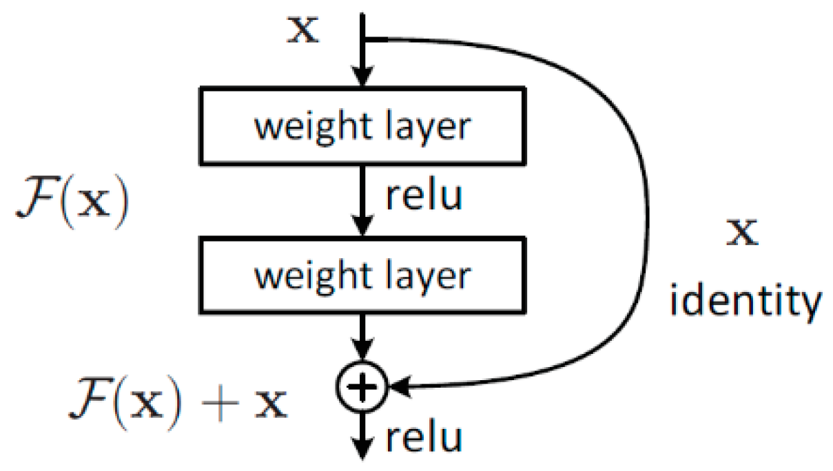
In terms of the above problems and training suitable deeper networks, many researchers introduced various structure networks, such as highway networks [30], stochastic depth [31], and FractalNets [32]. The advantage of these networks is to solve the problem by using a shortcut connection between the input and the output without more non-linear transformations. The authors of [33] introduce a residual block (Figure 1) and plug a skip connection to summarize the input and the output. can be expressed as:
where is the repetition (2 or 3 times) of a block combined with BN, followed by ReLUs and a Conv. With the shortcut connection, the gradient can flow from the deep layer to the shallow layer in the backpropagation, which can avoid a vanishing gradient. So, a network with more than one thousand layers with residual blocks can achieve the convergence aim.
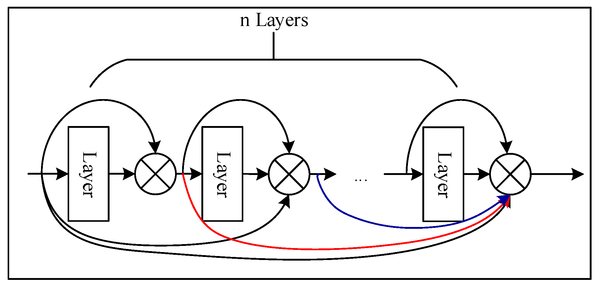
In terms of promoting the flow of information and gradients through the whole network, DenseNets [34] introduces a new connection pattern among layers (Figure 2). The dense block connects each layer in feed-forward fashion instead of the residual block. The feature maps of all preceding layers can be taken as inputs, and the inputs are put into the subsequent layers by concatenation. Different from ResNets, the network combined all feature maps by concatenation instead of summation, to avoid impeding information flow. Consequently, the layer obtains the outputs of the total preceding layers, , which are taken as inputs, and the output can be expressed as:
where indicates the concatenation of the feature maps in layers . So, is a composite function with BN, followed by ReLUs and a Conv. Because of its dense connectivity, DenseNets can exploit the network potential through feature reuse. Then, the output dimension for each layer, , has feature maps, and refers to the growth rate parameter, which can be set to a small value (e.g., ) [26].
Figure 2 shows that an input, , may be the input image at the initial position of the network or the end of the last layer, and an output feature map, , with channels is computed by applying the transformation function, . Further, is stacked to the previous feature map, , by concatenation (i.e., ) and taken as input to the next layer. The similar operation is repeated times and presents a dense block with feature maps (Figure 3).
The concatenation operation can bring more inputs, because convolution has been introduced in the network as a bottleneck layer before each convolution for decreasing the number of input feature maps [20,29], which can develop computational efficiency. So, the dense block adopts a bottleneck design and produces feature maps, and can be referred to as BN-ReLU-Conv()-BN-ReLU-Conv().
2.2. The Construction of the D-Dense Block
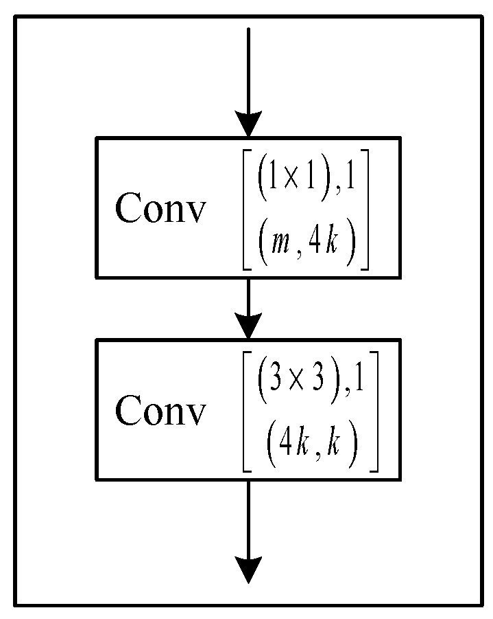
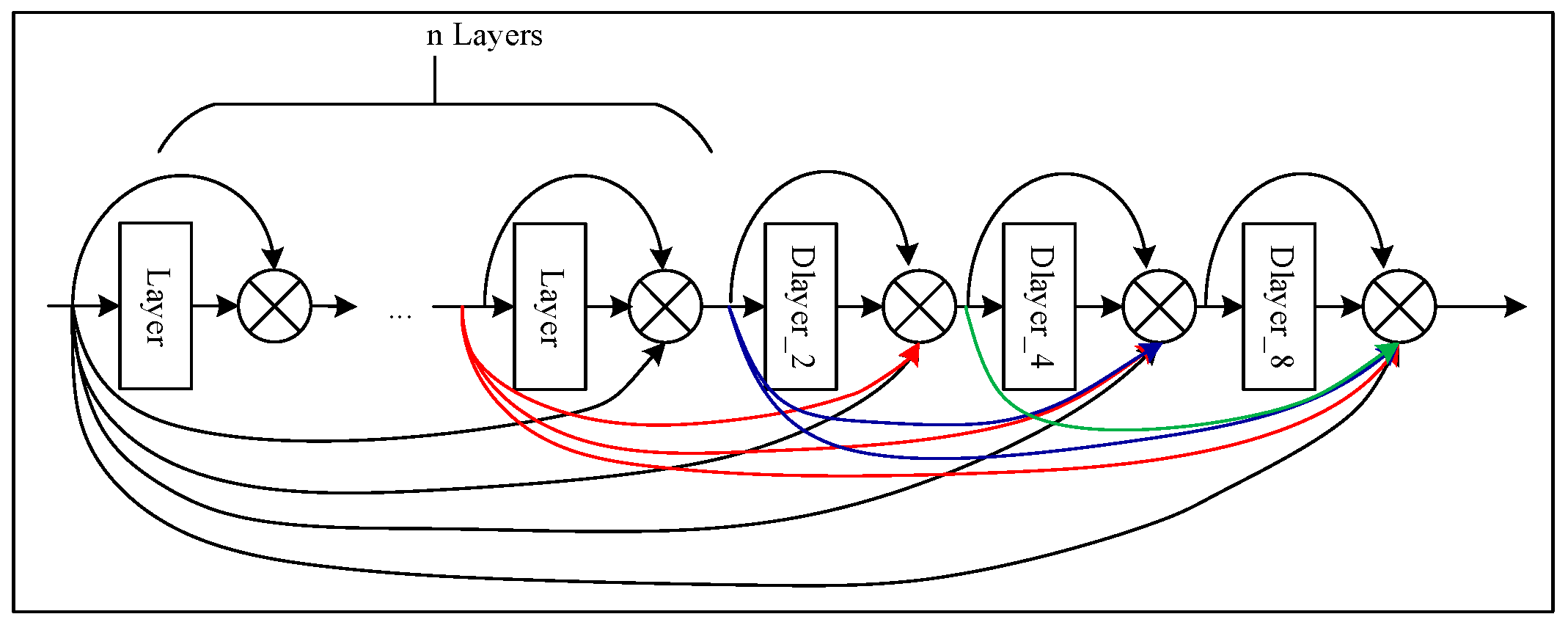
Three consecutive dilated convolution layers are plugged after the original dense block, and each layer has its expanding rate (2, 4 and 8) (Figure 4). Each dilated convolution is set as BN-ReLU-Conv (1 × 1)-BN-ReLU-D_Conv. The computing process iterates n plus 3 times, then the D-Dense block generates feature maps by using channels (n + 3) × k.
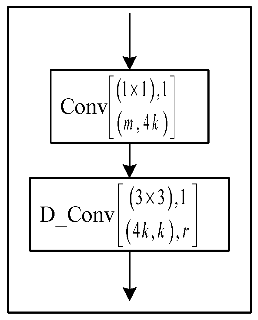
Each D-layer structure is shown in Figure 5. Here, r represents the expanding rate of dilated convolution.
2.3. The Structure of the Stem Block
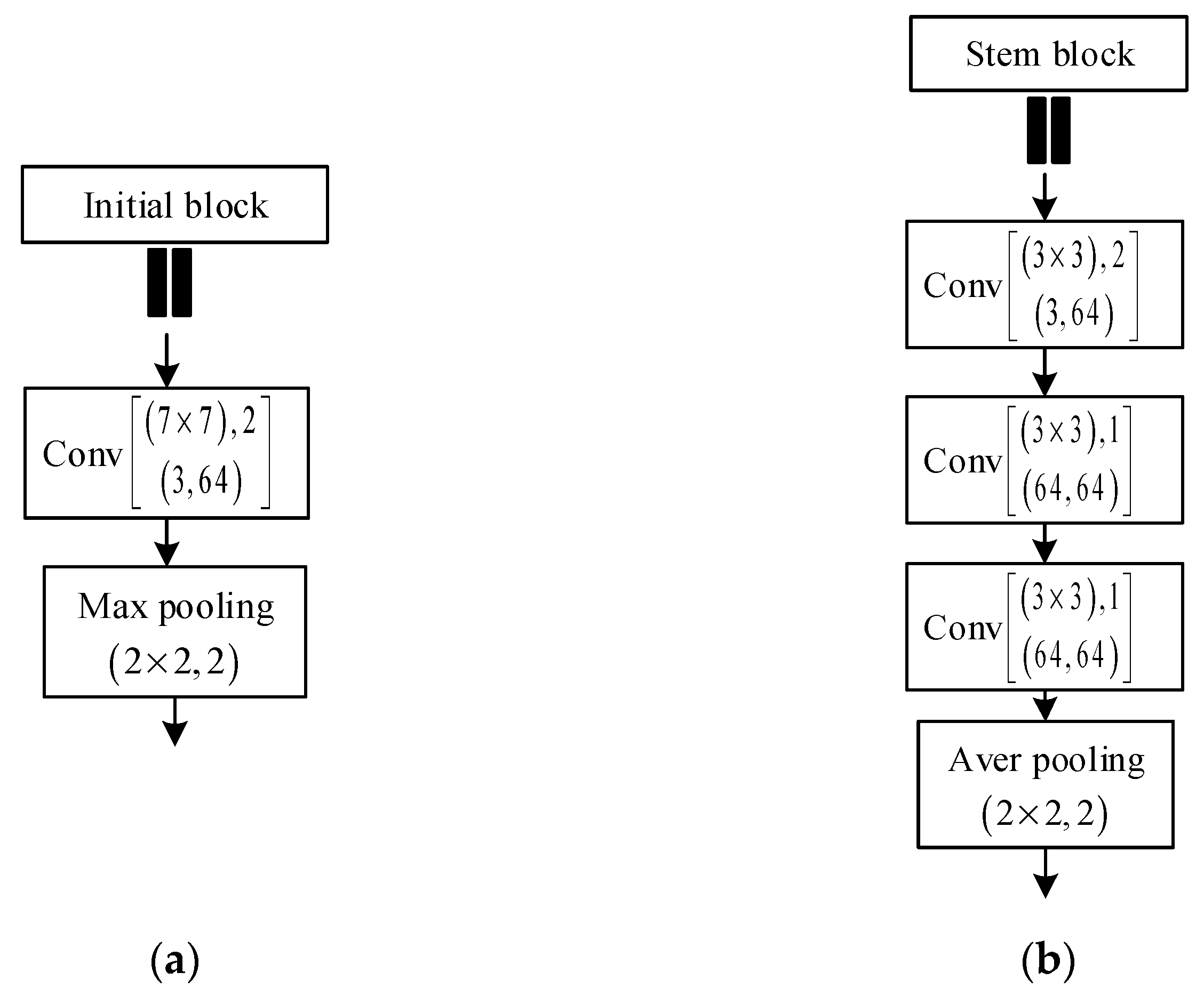
The encoder path can be listed as follows: first, an initial block operates; second, convolution performs on the input image with a kernel and 2 strides with max pooling. Further, the output channels are set as 64, and the stem block is arranged instead of the initial block [35,36,37,38]. The stem block is set as three convolution layers (3 × 3) and one mean pooling layer (2 × 2). There are 2 strides in the first convolution layer compared with only 1 of others. Meanwhile, the output channels for each convolution layers are set as 64. The authors of [38] have demonstrated that the initial block would lose information after two operations of consecutive down-sample, which is unable to recover the marginal feature in the decoder phase. Since the stem block is good at detecting objects, even small objects, the stem block is arranged as the initial position through the encoder phase. The differences between initial and stem blocks are shown in Figure 6.
2.4. Architecture of Semantic Segmentation Network
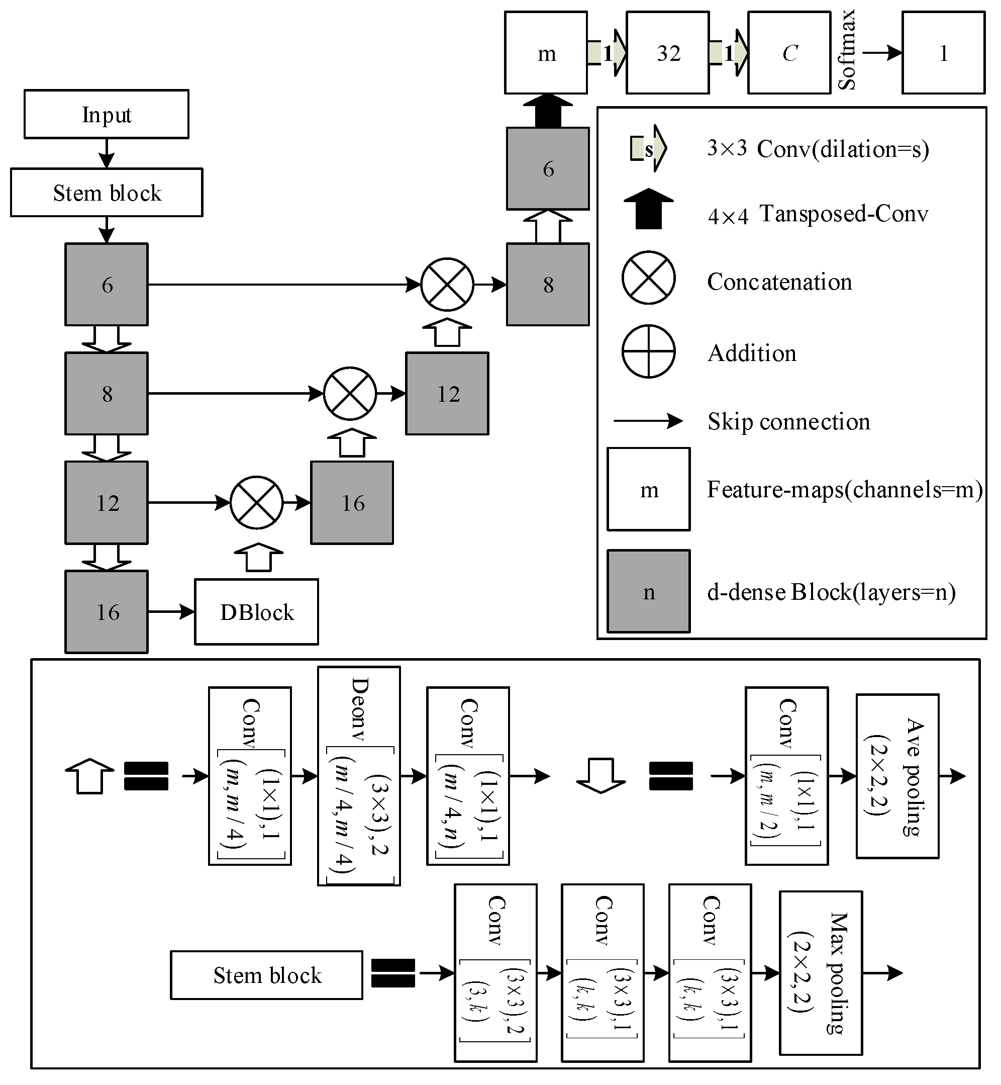
Here, the improved CNN with D-Dense block construction is named D-DenseNet (Figure 7). We introduce D-Block, the center part of D-LinkNet, into our improved network. Further, the proposed network uses a DenseNet backbone and took stem as the initial block.
The symbol in Figure 7 indicates that convolution kernel size is , stride is , the input channel is and the output channel is . The Conv in Figure 7 indicates BN-ReLU—Conv except the final convolution layer. In addition, Deconv is BN-ReLU-Transposed-Conv.
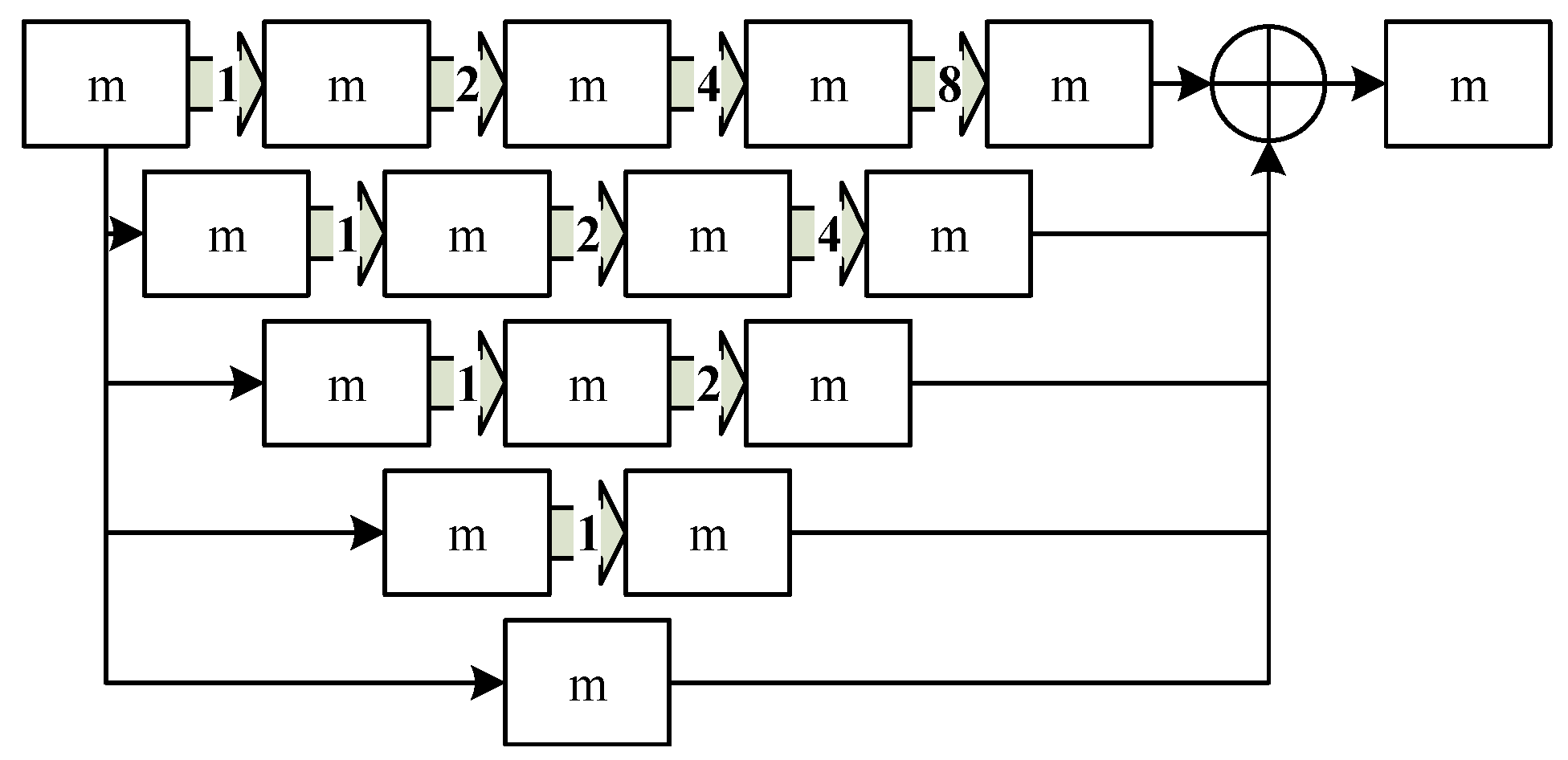
D-Block contains four steps (Figure 8): the dilated convolution of 2 cascade modes and 2 parallel modes. Meanwhile, different dilated convolutions have different expanding rates. Further, each path presents different receptive fields, and the multi-scale context information can be obtained.
3. Experiments
The research experiments are performed on the processing dataset and the public Massachusetts Road Dataset [39], respectively. The deep learning framework selects TensorFlow as the platform to train and test the relative networks. In addition, two sets of NVIDIA GTX 2080 Ti GPU are bridged to guarantee computing power.
3.1. Datasets
The method is evaluated with the processing team dataset from the WorldView-4 satellite, including 6736 training images with a spatial resolution of 0.31 m and 1012 similar test images. After data augmentation including color jittering, horizontal flip and vertical flip, the image is processed as 1024 × 1024. Finally, this research obtains 47,152 training images.
Further, we train and test the D-DenseNet on the Massachusetts Road Dataset [39] with 1108 training images, 14 validation images and 49 test images. Since the image size is , we cut the images into 1024 × 1024 because of memory limitations. The area in an image is labeled as the foreground for roads and the background for other. Then, the data are processed for the experiment.
3.2. Hybrid Loss Function
In previous research, only cross-entropy loss was applied for training models, which is defined as:
Here, means categories. and indicate the label and prediction vectors, respectively. The hybrid loss function can be defined as:
Here, represents regularization loss in the improved network. indicates binary cross-entropy loss with training images. represents the prediction result, while is the label image. In addition, shows the difference between prediction and label images on the pixel level. indicates the weight (set to approximately 0.7) in terms of total loss.
3.3. Implementation Details
The method from [40] is selected as our optimizer. During the training period, the learning rate is set as 0.0001, which would be decreased 10 times after the loss value, decreasing slowly. In addition, the batch size in the training phase is set as 2.
4. Results and Discussion
4.1. Results on the Processing Datesets
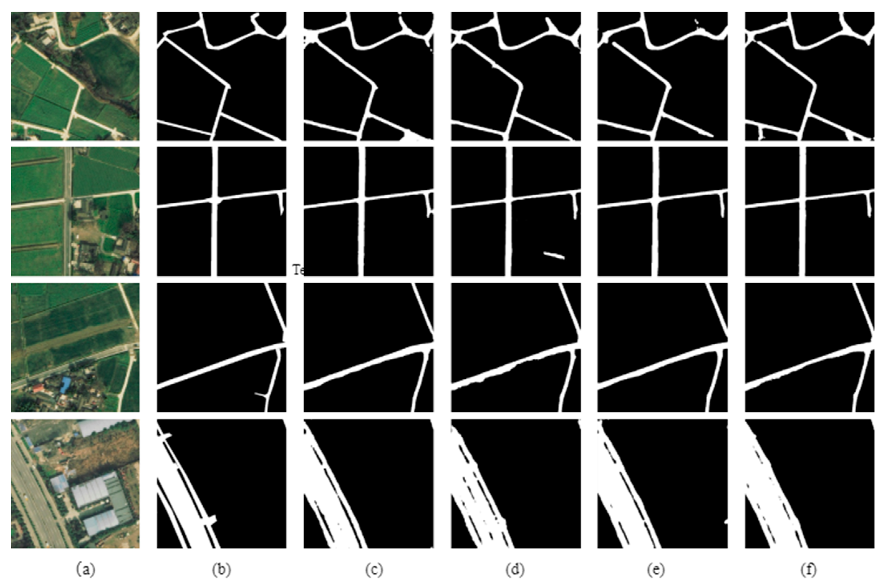
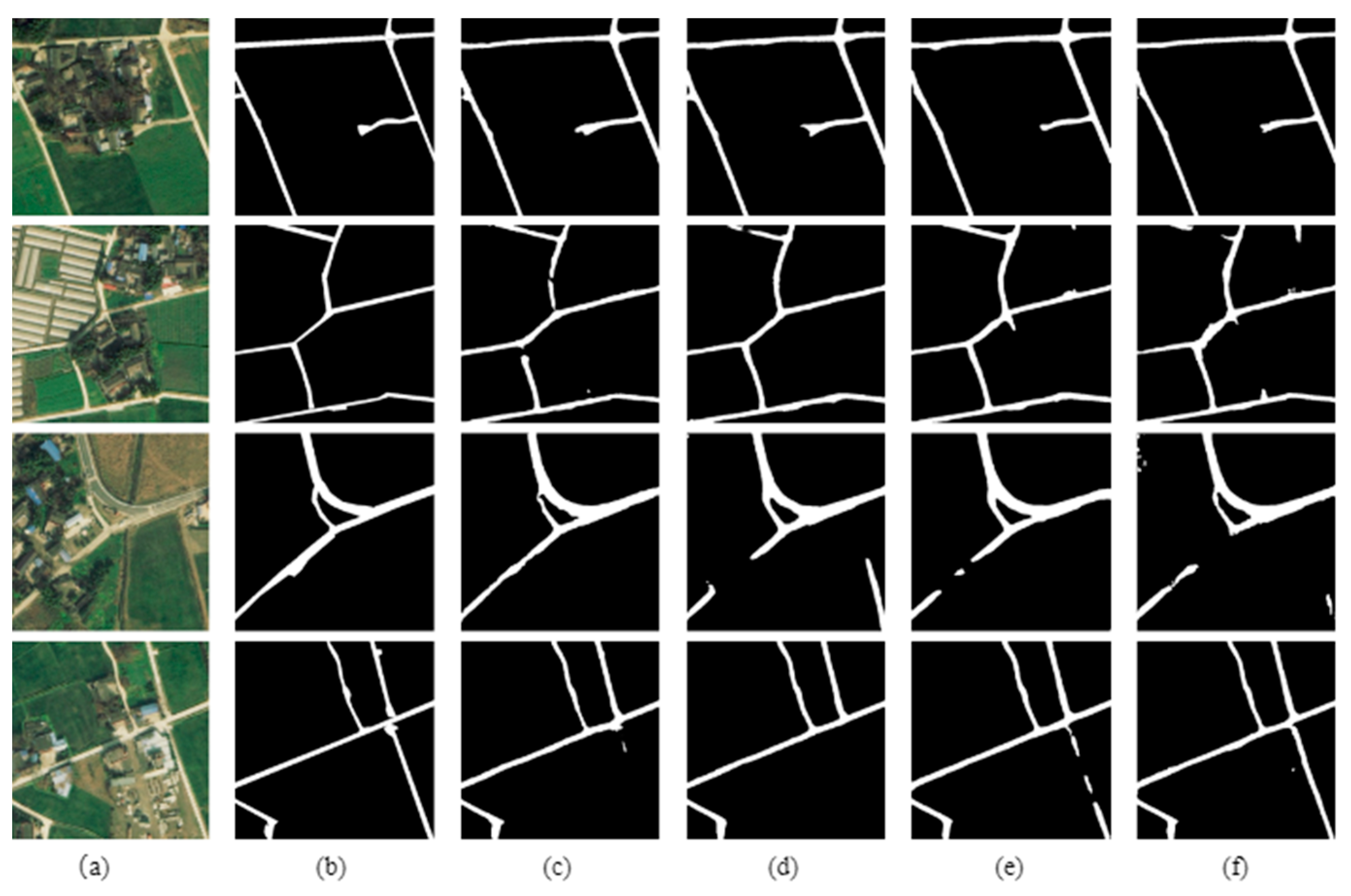
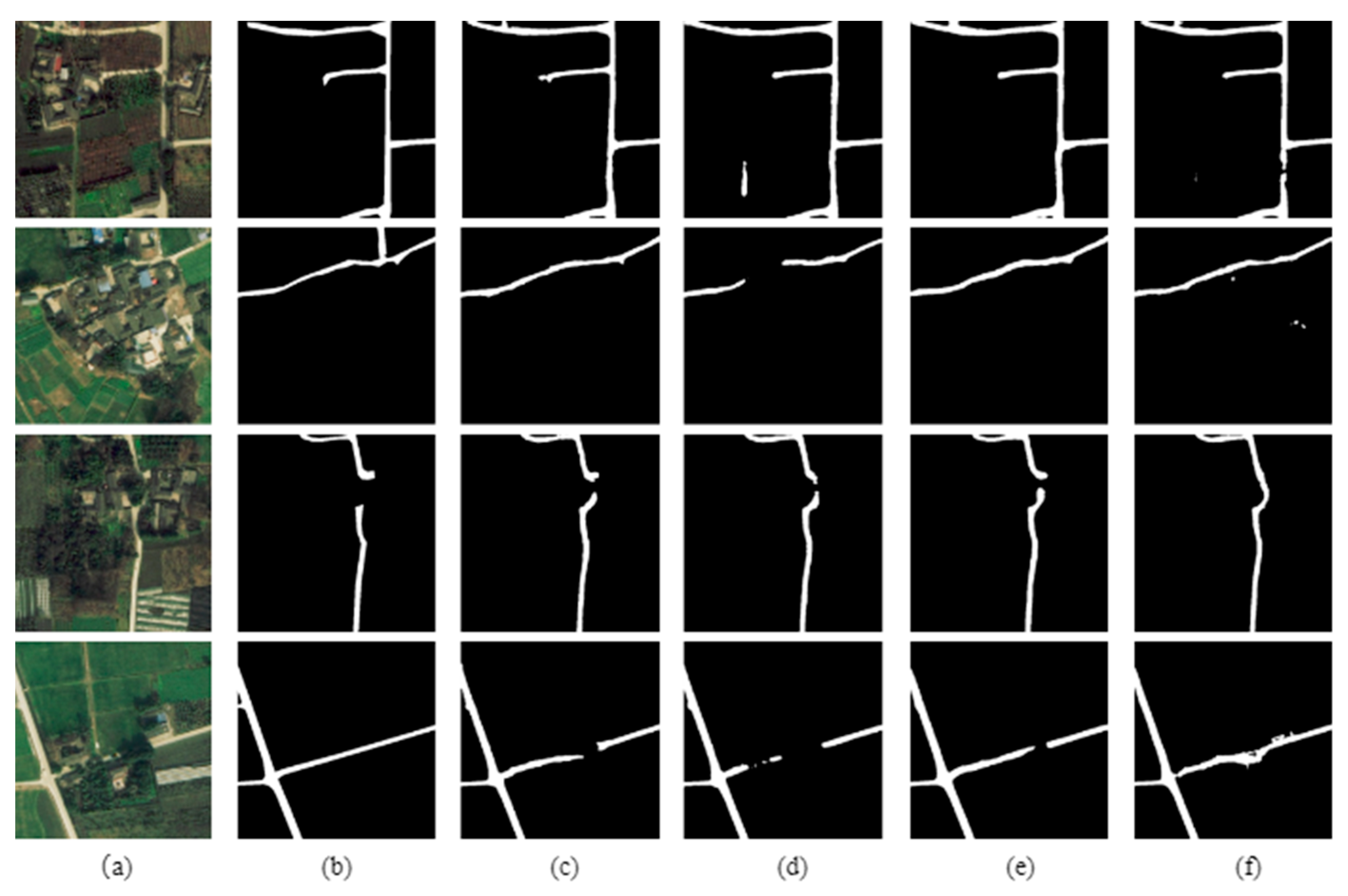
The processing dataset is divided into simple, general and complex scenes, following the position of the image contents. The three-level samples are shown in Figure 9, Figure 10 and Figure 11, respectively.
The road areas are highlighted in the simple scenes, and only a tiny part of the road areas is covered by shadows. The road areas around the building groups and some parts of the road areas are covered by buildings, trees and shadows in the general scenes. Greenhouses and buildings have similar features to the road, which will affect road area extraction. Large parts of the road are sheltered by trees and shadows in the complex scenes, which increases the difficulty of road extraction. The objective of these experiments is to obtain the model size and IoU of each network with different layers. Then, we can determine whether the proposed network is effective for precision (IoU) and computing power consumption (model size).
All networks selected in this research have effective performance for road extraction in the simple scenes. The road areas are extracted precisely and almost closed to the labels. We selected four networks to extract roads from satellite images. In the experiment, the number of layers for D-LinkNet is 101, while, for other networks, the number of layers is set as 24. In the simple scenes, the difference is not obvious. For Figure 10, all networks did not recognize the highlighted greenhouses or highlighted buildings as road areas. However, there are several road interruptions because of the shelters, especially in the third-row images. Only D-LinkNet (101) can extract the road areas covered by trees. In contrast to the fourth-column results and the fifth-column results in Figure 11, we find that the effect of the stem block is better prediction than that of the initial block. In addition, long distance road areas can also connect according to the context, while D-DenseNet (k = 24) + stem block is the best.
In terms of the improvement of road extraction accuracy for the improved network, various networks with D-Block are shown in Figure 7. The model size and IoU score of different networks are shown in Table 1. D-LinkNet (k = m) indicates that the selected network is constucted with a residual block and an encoder path has m convolutional layers, DenseNet (k = m) indicates that the network was constructed with the dense block and the growth_rate is m, and D-DenseNet (k = m) indicates that the network was constructed with the D-Dense block and the growth_rate is m. These networks built on the dense block have a smaller model size and a higher IoU score than those with a residual block. Further, the networks with a stem block have a smaller model size and a higher IoU score than that of the networks with an initial block. A smaller model scale can make the computation more efficient. The results show that D-DenseNet shows better performance with a similar model size.
4.2. Results Using the Public Dataset
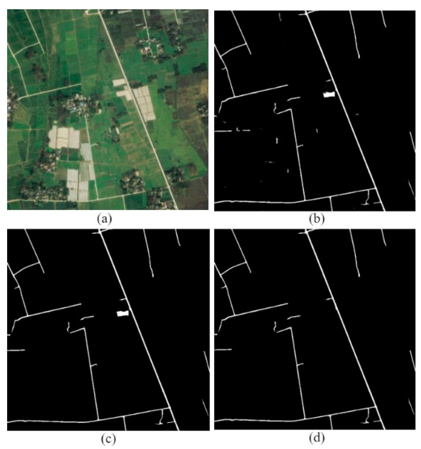
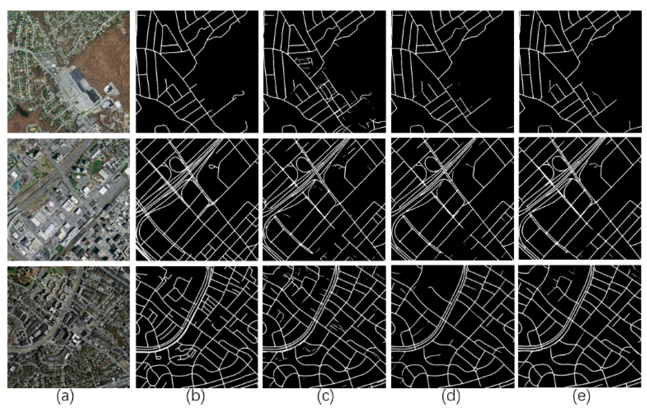
To further verify the effectiveness of the proposed improved network, the Massachusetts Roads Dataset was also applied for network evaluation. The test images are divided into two levels—general and complex scenes—following the position of the image contents. The sample results of the two-level images are shown in Figure 12 and Figure 13.
For the complicated scenes (Figure 13), the road area includes various-level roads and flyover roads, which would seriously affect the results from each network model. However, D-DenseNet (k = 24) + stem block + D-Block shows better performance for extraction including for the shadow-covered road.
After the experiments of model training and test, D-LinkNet, DenseNet and D-DenseNet model size and IoU index were collected (Table 2). We found that the model size of the network (the Dense-block and the D-Dense block) is much smaller than of those with the initial block. Further, a lower size obtains higher IoU scores. In addition, the improved D-DenseNet (k = 24) with D-Block has higher IoU scores than other networks, as shown in Table 2.
5. Conclusions
Deep learning has been applied in various fields, and road extraction was developed with convolutional neural networks. This research proposes improved networks, D-DenseNets, for reducing model size and increasing IoU scores. For the structure of the improved networks, a D-Dense block module was proposed according to the dense connection structure. In addition, D-DenseNet was constructed for semantic segmentation by using D-LinkNet as the center part with a D-Dense block. Meanwhile, D-DenseNet also introduced a stem block instead of an initial block for obtaining more detailed information. The two datasets were used to build and evaluate. Low-level road extraction from the team dataset of the WorldView-4 satellite showed that D-DenseNet (k = 24) + stem block has the highest IoU score and a smaller size compared with the selected models. Further, the results from public datasets showed that D-DenseNet not only the best IoU scores and a smaller size, but better performance for extraction in complicated scenes. The two experiment results show that the proposed D-DenseNet based on the D-Dense block shows better performance than the original D-LinkNet and DenseNet in terms of IoU scores and model size. So, the improved network can be applied for low-level road extraction.
In terms of model size and IoU scores, the function of each part of the network is the next research area, and each hyperparameter in the training phase should be carefully considered. Meanwhile, some postprocessing methods should be introduced to improve the quality of output images, which are still necessary for further processing to improve the presentation quality of low-level road extraction.
Author Contributions
Conceptualization, L.H.; formal analysis, L.H. and Y.L.; funding acquisition, D.T.; investigation, B.P.; methodology, Y.L.; resources, Y.L.; software, B.P.; supervision, D.T.; validation, B.P.; writing—original draft, L.H.; writing—review and editing, L.H. and D.T. All authors have read and agreed to the published version of the manuscript.
Funding
The Key Projects from the Ministry of Science and Technology of China (No. 2020YFA0608203); the Science & Technology Plan Project of Sichuan Province (NO 2021YFS0335).
Institutional Review Board Statement
Not applicable.
Informed Consent Statement
Not applicable.
Data Availability Statement
The data in the research is available. Please contact the corresponding author by sending e-mail to [email protected].
Conflicts of Interest
The authors declare no conflict of interest.
References
- Zheng, W.; Liu, X.; Yin, L. Research on image classification method based on improved multi-scale relational network. PeerJ Comput. Sci. 2021, 7, e613. [Google Scholar] [CrossRef] [PubMed]
- Wei, Y.; Zhang, K.; Ji, S. Simultaneous Road Surface and Centerline Extraction From Large-Scale Remote Sensing Images Using CNN-Based Segmentation and Tracing. IEEE Trans. Geosci. Remote Sens. 2020, 58, 8919–8931. [Google Scholar] [CrossRef]
- Wu, X.; Liu, Z.; Yin, L.; Zheng, W.; Song, L.; Tian, J.; Yang, B.; Liu, S. A Haze Prediction Model in Chengdu Based on LSTM. Atmosphere 2021, 12, 1479. [Google Scholar] [CrossRef]
- Zheng, W.; Yin, L. Characterization inference based on joint-optimization of multi-layer semantics and deep fusion match-ing network. PeerJ Comput. Sci. 2022, 8, e908. [Google Scholar] [CrossRef] [PubMed]
- Simonyan, K.; Zisserman, A. Very deep convolutional networks for large-scale image recognition. arXiv 2014, arXiv:1409.1556. [Google Scholar]
- Yu, F.; Koltun, V. Multi-scale context aggregation by dilated convolutions. arXiv 2015, arXiv:1511.07122. [Google Scholar]
- Zhou, L.; Zhang, C.; Wu, M. D-linknet: Linknet with pretrained encoder and dilated convolution for high resolution satel-lite imagery road extraction. In Proceedings of the IEEE Conference on Computer Vision and Pattern Recognition Work-Shops, San Juan, PR, USA, 17–19 June 1997; pp. 182–186. [Google Scholar]
- Chaurasia, A.; Culurciello, E. LinkNet: Exploiting Encoder Representations for Efficient Semantic Segmentation. arXiv 2017, arXiv:1707.03718v1. [Google Scholar]
- Farabet, C.; Couprie, C.; Najman, L.; LeCun, Y. Learning hierarchical features for scene labeling. IEEE Trans. Pattern Anal. Mach. Intell. 2013, 35, 1915–1929. [Google Scholar] [CrossRef] [Green Version]
- Pinheiro, P.H.O.; Collobert, R. Recurrent convolutional neural networks for scene labeling. Proc. Mach. Learn. Res. 2014, 32, 82–90. [Google Scholar]
- Badrinarayanan, V.; Kendall, A.; Cipolla, R. Segnet: A deep convolutional encoder-decoder architecture for image segmenta-tion. IEEE Trans. Pattern Anal. Mach. Intell. 2017, 39, 2481–2495. [Google Scholar] [CrossRef]
- Chen, L.C.; Papandreou, G.; Kokkinos, I.; Murphy, K.; Yuille, A.L. Deeplab: Semantic image segmentation with deep convolutional nets, atrous convolution, and fully connected crfs. IEEE Trans. Pattern Anal. Mach. Intell. 2018, 40, 834–848. [Google Scholar] [CrossRef] [PubMed] [Green Version]
- Lin, G.; Milan, A.; Shen, C.; Reid, I. RefineNet: Multi-path refinement networks with identity mappings for high-resolution se-mantic segmentation. arXiv 2016, arXiv:1611.06612. [Google Scholar]
- Chen, L.C.; Zhu, Y.; Papandreou, G.; Schroff, F.; Adam, H. Encoder-decoder with atrous separable convolution for semantic image segmentation. In Proceedings of the European Conference on Computer Vision (ECCV), Munich, Germany, 8–14 September 2018; pp. 801–818. [Google Scholar]
- Zhao, H.; Shi, J.; Qi, X.; Wang, X.; Jia, J. Pyramid scene parsing network. In Proceedings of the IEEE Conference on Computer Vision and Pattern Recognition, Honolulu, HI, USA, 21–26 July 2017; pp. 2881–2890. [Google Scholar]
- Li, Y.; Peng, B.; He, L.; Fan, K.; Tong, L. Road Segmentation of Unmanned Aerial Vehicle Remote Sensing Images Using Adversarial Network With Multiscale Context Aggregation. IEEE J. Sel. Top. Appl. Earth Obs. Remote Sens. 2019, 12, 2279–2287. [Google Scholar] [CrossRef]
- Zhou, M.; Sui, H.; Chen, S.; Wang, J.; Chen, X. BT-RoadNet: A boundary and topologically-aware neural network for road extraction from high-resolution remote sensing imagery. ISPRS J. Photogramm. Remote Sens. 2020, 168, 288–306. [Google Scholar] [CrossRef]
- Chen, Z.; Wang, C.; Li, J.; Xie, N.; Han, Y.; Du, J. Reconstruction Bias U-Net for Road Extraction From Optical Remote Sens-ing Images. IEEE J. Sel. Top. Appl. Earth Obs. Remote Sens. 2021, 14, 2284–2294. [Google Scholar] [CrossRef]
- Dey, M.S.; Chaudhuri, U.; Banerjee, B.; Bhattacharya, A. Dual-Path Morph-UNet for Road and Building Segmentation From Satellite Images. IEEE Geosci. Remote Sens. Lett. 2021, 19, 1–5. [Google Scholar] [CrossRef]
- Zheng, W.; Tian, X.; Yang, B.; Liu, S.; Ding, Y.; Tian, J.; Yin, L. A few shot classification methods based on multiscale relational networks. Appl. Sci. 2022, 12, 4059. [Google Scholar] [CrossRef]
- Geng, Q.; Zhang, H.; Qi, X.; Huang, G.; Yang, R.; Zhou, Z. Gated Path Selection Network for Semantic Segmentation. IEEE Trans. Image Process. 2021, 30, 2436–2449. [Google Scholar] [CrossRef]
- Ioffe, S.; Szegedy, C. Batch normalization: Accelerating deep network training by reducing internal covariate shift. arXiv 2015, arXiv:1502.03167. [Google Scholar]
- Glorot, X.; Bordes, A.; Bengio, Y. Deep sparse rectifier neural networks. In Proceedings of the Fourteenth International con-Ference on Artificial Intelligence and Statistics, Fort Lauderdale, FL, USA, 11–13 April 2011; pp. 315–323. [Google Scholar]
- LeCun, Y.; Bottou, L.; Bengio, Y.; Haffner, P. Gradient-based learning applied to document recognition. Proc. IEEE 1998, 86, 2278–2324. [Google Scholar] [CrossRef]
- Srivastava, N.; Hinton, G.; Krizhevsky, A.; Sutskever, H.; Salakhutdinov, R. Dropout: A simple way to prevent neural networks from overfitting. J. Mach. Learn. Res. 2014, 15, 1929–1958. [Google Scholar]
- Jégou, S.; Drozdzal, M.; Vazquez, D.; Romero, A.; Bengio, Y. The one hundred layers tiramisu: Fully convolutional densenets for semantic segmentation. In Proceedings of the IEEE Conference on Computer Vision and Pattern Recognition Workshops, Honolulu, HI, USA, 21–26 July 2017; pp. 11–19. [Google Scholar]
- Cun, Y.L.; Bottou, L.; Orr, G.; Muller, K. Efficient backprop. In Neural Networks: Tricks of the Trade; Springer: Berlin/Heidelberg, Germany, 2012; pp. 9–48. [Google Scholar]
- Glorot, X.; Bengio, Y. Understanding the difficulty of training deep feedforward neural networks. In Proceedings of the Thirteenth International Conference on Artificial Intelligence and Statistics, Sardinia, Italy, 13–15 May 2010; pp. 249–256. [Google Scholar]
- He, K.; Zhang, X.; Ren, S.; Sun, J. Delving deep into rectifiers: Surpassing human-level performance on imagenet classification. In Proceedings of the IEEE International Conference on Computer Vision, Santiago, Chile, 7–13 December 2015; pp. 1026–1034. [Google Scholar]
- Srivastava, R.K.; Greff, K.; Schmidhuber, J. Highway networks. arXiv 2015, arXiv:1505.00387. [Google Scholar]
- Huang, G.; Sun, Y.; Liu, Z.; Sedra, D.; Weinberger, K.Q. Deep networks with stochastic depth. In European Conference on Computer Vision; Springer: Berlin/Heidelberg, Germany, 2016; pp. 646–661. [Google Scholar]
- Larsson, G.; Maire, M.; Shakhnarovich, G. Fractalnet: Ultra-deep neural networks without residuals. arXiv 2016, arXiv:1605.07648. [Google Scholar]
- He, K.; Zhang, X.; Ren, S.; Sun, J. Deep residual learning for image recognition. In Proceedings of the IEEE Conference on Computer Vision and Pattern Recognition, Las Vegas, NV, USA, 27–30 June 2016; pp. 770–778. [Google Scholar]
- Huang, G.; Liu, Z.; Van Der Maaten, L.; Weinberger, K.Q. Densely connected convolutional networks. In Proceedings of the IEEE Conference on Computer Vision and Pattern Recognition, Honolulu, HI, USA, 21–26 July 2017; pp. 4700–4708. [Google Scholar]
- Szegedy, C.; Vanhoucke, V.; Ioffe, S.; Shlens, J.; Wojna, Z. Rethinking the inception architecture for computer vision. In Proceedings of the IEEE Conference on Computer Vision and Pattern Recognition, Las Vegas, NV, USA, 27–30 June 2016; pp. 2818–2826. [Google Scholar]
- Szegedy, C.; Ioffe, S.; Vanhoucke, V.; Alemi, A.A. Inception-v4, inception-resnet and the impact of residual connections on learning. In Proceedings of the Thirty-First AAAI Conference on Artificial Intelligence 2017, San Francisco, CA, USA, 4–9 February 2017. [Google Scholar]
- Shen, Z.; Liu, Z.; Li, J.; Jiang, Y.G.; Chen, Y.; Xue, X. Dsod: Learning deeply supervised object detectors from scratch. In Proceedings of the IEEE Inter-national Conference on Computer Vision, Venice, Italy, 22–29 October 2017; pp. 1919–1927. [Google Scholar]
- Zhou, P.; Ni, B.; Geng, C.; Hu, J.; Xu, Y. Scale-transferrable object detection. In Proceedings of the IEEE Conference on Computer Vi-sion and Pattern Recognition, Salt Lake City, UT, USA, 18–23 June 2018; pp. 528–537. [Google Scholar]
- Demir, I.; Koperski, K.; Lindenbaum, D.; Pang, G.; Huang, J.; Basu, S.; Hughes, F.; Tuia, D.; Raskar, R. Deepglobe 2018: A challenge to parse the earth through satellite images. In Proceedings of the 2018 IEEE/CVF Conference on Computer Vision and Pattern Recognition Workshops (CVPRW), Salt Lake City, UT, USA, 18–22 June 2018; pp. 172–17209. [Google Scholar]
- Kingma, D.P.; Ba, J. Adam: A method for stochastic optimization. arXiv 2014, arXiv:1412.6980. [Google Scholar]
Figure 1.
The structure of the residual block [33].
Figure 1.
The structure of the residual block [33].

Figure 2.
The structure of the dense block.

Figure 3.
The structure of each layer.

Figure 4.
D-Dense block construction.

Figure 5.
The construction of the D-layer.

Figure 6.
Relation between initial and stem blocks: (a) the initial block; (b) the stem block.

Figure 7.
The proposed network construction with the D-Dense block.

Figure 8.
The construction of D-Block.

Figure 9.
Results in the simple scenes: (a) original images; (b) labels; (c) D-LinkNet (101); (d) DenseNet (k = 24) + initial block; (e) DenseNet (k = 24) + stemblock; (f) D-DenseNet (k = 24) + stem block.
Figure 9.
Results in the simple scenes: (a) original images; (b) labels; (c) D-LinkNet (101); (d) DenseNet (k = 24) + initial block; (e) DenseNet (k = 24) + stemblock; (f) D-DenseNet (k = 24) + stem block.

Figure 10.
Results in the general scenes: (a) original images; (b) labels; (c) D-LinkNet (101); (d) DenseNet (k = 24) + initial block; (e) DenseNet (k = 24) + stem block; (f) D-DenseNet (k = 24) + stem block.
Figure 10.
Results in the general scenes: (a) original images; (b) labels; (c) D-LinkNet (101); (d) DenseNet (k = 24) + initial block; (e) DenseNet (k = 24) + stem block; (f) D-DenseNet (k = 24) + stem block.

Figure 11.
Results in the complex scenes: (a) original images; (b) labels; (c) D-LinkNet (101); (d) DenseNet (k = 24) + initial block; (e) DenseNet (k = 24) + stem block; (f) D-DenseNet (k = 24) + stem block.
Figure 11.
Results in the complex scenes: (a) original images; (b) labels; (c) D-LinkNet (101); (d) DenseNet (k = 24) + initial block; (e) DenseNet (k = 24) + stem block; (f) D-DenseNet (k = 24) + stem block.

Figure 12.
Results in the general scenes: (a) original image; (b) label; (c) D-LinkNet; (d) DenseNet (k = 24) + stem block.
Figure 12.
Results in the general scenes: (a) original image; (b) label; (c) D-LinkNet; (d) DenseNet (k = 24) + stem block.

Figure 13.
Results in the complicated scenes: (a) original image; (b) label; (c) D-LinkNet; (d) DenseNet (k = 24) + stem block; (e) D-DenseNet (k = 24) + stem block + D-Block.
Figure 13.
Results in the complicated scenes: (a) original image; (b) label; (c) D-LinkNet; (d) DenseNet (k = 24) + stem block; (e) D-DenseNet (k = 24) + stem block + D-Block.


Table 1.
Results on our test set of different models.
| Model’s Description | Model Size (MB) | IoU (%) |
|---|---|---|
| D-LinkNet (50) + Initial Block + D-Block | 792 | 51.370 |
| D-LinkNet (101) + Initial Block + D-Block | 980 | 52.360 |
| DenseNet (k = 24) + Initial Block + D-Block | 82.6 | 55.420 |
| DenseNet (k = 32) + Initial Block + D-Block | 139 | 53.390 |
| DenseNet (k = 24) + Stem Block + D-Block | 81.7 | 55.580 |
| DenseNet (k = 32) + Stem Block + D-Block | 137 | 54.610 |
| D-DenseNet (k = 24) + Stem Block + D-Block | 119 | 57.960 |
| D-DenseNet (k = 32) + Stem Block + D-Block | 152 | 57.650 |
Table 2.
Results using the public dataset for selected models.
| Model’s Description | Model Size (MB) | IoU (%) |
|---|---|---|
| D-LinkNet (101) + initial block + D-Block | 1.070 | 63.10 |
| DenseNet (k = 24) + stem block + D-Block | 82.4 | 64.38 |
| DenseNet (k = 32) + stem block + D-Block | 111 | 63.02 |
| D-DenseNet (k = 24) + stem block + D-Block | 99.3 | 66.28 |
| D-DenseNet (k = 32) + stem block + D-Block | 169 | 65.25 |
Publisher’s Note: MDPI stays neutral with regard to jurisdictional claims in published maps and institutional affiliations. |
© 2022 by the authors. Licensee MDPI, Basel, Switzerland. This article is an open access article distributed under the terms and conditions of the Creative Commons Attribution (CC BY) license (https://creativecommons.org/licenses/by/4.0/).
Share and Cite
MDPI and ACS Style
He, L.; Peng, B.; Tang, D.; Li, Y. Road Extraction Based on Improved Convolutional Neural Networks with Satellite Images. Appl. Sci. 2022, 12, 10800. https://0-doi-org.brum.beds.ac.uk/10.3390/app122110800
AMA Style
He L, Peng B, Tang D, Li Y. Road Extraction Based on Improved Convolutional Neural Networks with Satellite Images. Applied Sciences. 2022; 12(21):10800. https://0-doi-org.brum.beds.ac.uk/10.3390/app122110800
Chicago/Turabian StyleHe, Lei, Bo Peng, Dan Tang, and Yuxia Li. 2022. "Road Extraction Based on Improved Convolutional Neural Networks with Satellite Images" Applied Sciences 12, no. 21: 10800. https://0-doi-org.brum.beds.ac.uk/10.3390/app122110800
Note that from the first issue of 2016, this journal uses article numbers instead of page numbers. See further details here.