An Interpretable Machine Learning Approach for Hepatitis B Diagnosis

Abstract

Hepatitis B is a potentially deadly liver infection caused by the hepatitis B virus. It is a serious public health problem globally. Substantial efforts have been made to apply machine learning in detecting the virus. However, the application of model interpretability is limited in the existing literature. Model interpretability makes it easier for humans to understand and trust the machine-learning model. Therefore, in this study, we used SHapley Additive exPlanations (SHAP), a game-based theoretical approach to explain and visualize the predictions of machine learning models applied for hepatitis B diagnosis. The algorithms used in building the models include decision tree, logistic regression, support vector machines, random forest, adaptive boosting (AdaBoost), and extreme gradient boosting (XGBoost), and they achieved balanced accuracies of 75%, 82%, 75%, 86%, 92%, and 90%, respectively. Meanwhile, the SHAP values showed that bilirubin is the most significant feature contributing to a higher mortality rate. Consequently, older patients are more likely to die with elevated bilirubin levels. The outcome of this study can aid health practitioners and health policymakers in explaining the result of machine learning models for health-related problems.

1. Introduction

Hepatitis B, a liver infection caused by the hepatitis B virus (HBV), has remained a public health issue globally [1,2,3]. HBV is spread when an infected person or a virus carrier has fluid contact with someone who is not infected. Recent studies show that HBV is 100 times more infectious than HIV/AIDS and remains the primary cause of liver cancer [4]. HBV has infected one out of every three persons, amounting to two billion people globally [1,3]. About 1.5 million people get infected annually, and over 300 million are chronically infected [1,2]. An estimated 820,000 people die annually from complications associated with HBV, and an average of two people die each minute from HBV [1,3,5]. Although enormous progress has been made on HPV vaccinations, many African and Asian countries are still regarded as high-endemicity areas, with the HPV prevalence in West Africa estimated at 8.83% [6]. Meanwhile, the high endemicity in developing countries was attributed to the low vaccinations among people over 18 years of age [7].

People infected with HBV need adequate treatment to remain healthy and alive. Despite effective prophylactic vaccine and diagnostic efforts, HBV remains a significant public health crisis with a high death toll  [8,9,10]. In recent times, antivirals have been shown to eliminate HBV infection, but cessation of therapy can lead to a rebound of the virus [10]. Early detection can help reduce its debilitating effects and minimize the risk of transmission through contact with an infected person’s blood and bodily fluids [11].

Conventional medical approaches to classify patients infected with HBV use different biochemical and virological factors to infer liver damage and viral activity [12]. Studies have also shown that other traditional statistical methods can predict acute and chronic HBV with clinical data [13,14,15]. Such predictions with the conventional statistical method could be biased due to the multicollinearity issue for high-dimensional medical data. Furthermore, in complex viral disease situations, where basic laboratory tests may not be a sufficient insight into the clinical history and patient progression, using advanced analytics, such as machine learning (ML) algorithms, may offer numerous advantages. These algorithms help unlock insights into the pathogen and host factors that can represent novel biomarkers for therapeutic and prognostic strategies. ML algorithms can identify patterns that show unknown relationships between covariates to be made about future events. However, machine learning algorithms have gained considerable attention in the medical health domain and have been used to address different medical-related problems [16,17,18,19,20]. Machine learning algorithms have been used effectively as a classification method to extract information from medical data to make accurate predictions for HBV diagnosis [21,22,23,24].

Many studies have utilized machine learning (ML) models to predict hepatitis B on clinical datasets. Tian et al. [25] applied several ML models for a better prognosis among patients suffering from chronic hepatitis B. The models were based on logistic regression (LR), decision tree (DCT), extreme gradient boosting (XGBoost), and random forest (RF). The study concluded that the ML models were effective and showed better predictive performance on available clinical data. In a similar study, Wübbolding et al. [26] applied the supervised, embedded ML methods using LR, support vector machine (SVM), and stochastic gradient descent (SGD) at several time points. The experimental results showed that SVM performed exceedingly well and obtained the best cross-validation accuracy. In an attempt to increase the accuracy of ML classifiers on a hepatitis B vaccination status dataset, Putri et al. [27] considered Synthetic Minority Oversampling Technique (SMOTE) to obtain balanced data and applied RF and Naïve Bayes (NB) for the prediction task. The result showed that the RF was more efficient for the prediction.

Predicting hepatitis B in clinical datasets is not only limited to conventional ML classifiers. Even several deep-learning methods have been proposed to address this issue. Kamimura et al. [28] used the deep neural network (DNN) to predict hepatitis B surface level antigen levels against statistical techniques. The study demonstrated that DNN offered better performance than statistical methods in predicting clinical outcomes. For a time-series forecasting of hepatitis B incidence, Xia et al. [29] applied three deep learning algorithms based on Long Short-Term Memory (LSTM) prediction model, Recurrent Neural Network (RNN) prediction model, and Back Propagation Neural Network (BPNN). The study concluded that deep learning techniques offered a significant predictive forecast for hepatitis incidences and could assist decision makers in disease control and management. However, to the best of our knowledge, the use of model interpretability in HPV detection studies is still limited.

Several ML studies in the literature did not consider model explainability; hence, the model outcomes cannot be adequately understood by medical practitioners and health policymakers. Meanwhile, interpreting ML models to understand the features that cause HBV infection could be beneficial in real-world applications and for stakeholders in the health sector. Consequently, the main contributions of this study include 1. building and optimizing ML algorithms toward effective HBV detection and diagnosis, 2. Introducing model explainability using SHapley Additive exPlanations (SHAP), a game-based theoretical approach aimed at explaining and visualizing the predictions of the ML models, 3. interpreting and ranking the HPV causative features. In essence, this study seeks to understand why a machine learning model makes a prediction and what features contribute to the decision. The machine learning algorithms used to develop HPV detection models include decision trees, logistic regression, support vector machine (SVM), random forest, XGBoost, and AdaBoost.

The remainder of the manuscript is organized as follows. Section 2 describes the proposed methods for data collection, pre-processing, and models used. Section 3 presents some experimental results. Section 4 presents the model interpretation. In Section 5, the discussion of this paper is presented. This study concludes in Section 6.

2. Materials and Methods

In this part, we present the dataset, the methods of data collection, and data prepossessing and describe some models used in this study.

2.1. Data Collection

The dataset used for this study was downloaded from the University of California Irvine (UCI) Machine Learning Repository [30,31]. The choice of the UCI Machine Learning Repository was because they maintain their datasets as a service to the machine learning community. The selection of hepatitis datasets from the UCI Machine Learning Repository in this work is strictly by choice, considering the scarcity of relevant data in this area of study. The dataset contains the demography and clinical records of 155 hepatitis B patients with 20 unique features. The features include class (died or lived), age, gender (male or female), steroid, antivirals, fatigue, malaise, anorexia, liver_big, and liver_firm. Others are spleen_palable, spiders, ascites, varices, bilirubin, alk_Phosphate, sgot, albumin, protime, and histology.

Table 1. Dataset description.

S/N	Attribute	Type	Description
1	Class = “Died”, “Lived”	Nominal	Patients that died or survived
2	Age	Numeric	Patient’s age
3	Gender	Nominal	Male or Female
4	Steroid	Nominal	Increases HBV replication
5	Antivirals	Nominal	Drugs to stop or slow replication of HBV
6	Fatigued	Nominal	Impairment of functional capabilities due to HBV
7	Malaise	Nominal	State of discomfort and unwell
8	Anorexia	Nominal	Loss of appetite
9	Liver_big	Nominal	Enlarged liver
10	Liver_firm	Nominal	Enlarged liver
11	Spleen_palable	Nominal	Enlarged spleen
12	Spiders	Nominal	Abnormal collection of blood vessels clustered near the skin surface
13	Ascites	Nominal	Abnormal accumulation of fluids in the abdomen
14	Varices	Nominal	Enlarged veins
15	Bilirubin	Numeric	Yellowship pigment formed after the breakdown of red blood cells.
16	Alk_Phosphate	Numeric	Used for screening fibrosis levels
17	Sgot	Numeric	Liver enzyme
18	Albumin	Numeric	Protein made by the liver
19	Protime	Numeric	Protein made by the liver
20	Histology	Nominal	Microscopy study of the liver

summarizes the description of the attributes. Next, we discuss the data processing technique used.

2.2. Data Preprocessing

In this study, the nested cross-validation (nested CV) procedure is employed to estimate the skill of the models. The nested CV is an essential method in the application of ML for medical diagnosis because of the limited data available for training ML models in the healthcare domain [32]. The nested cross-validation method is a double cross-validation technique, where the k-fold cross-validation for model hyperparameter tuning is nested inside the k-fold cross-validation for model selection. Model selection without nested CV applies the same data to tune the model and evaluate performance, which could result in data leakage and overfitting.

The k-fold cross-validation method entails training a model using all folds except one and testing the trained model using the holdout fold. Assuming that the combination of folds used to fit the model is called the training dataset and the held-out fold is the test dataset, then each training dataset is coupled with the grid search optimization technique to obtain the best hyperparameter combination for the model. Meanwhile, another k-fold cross-validation is employed to evaluate the hyperparameter combinations, and it divides the previously obtained training dataset into k-folds [33]. Therefore, the nested CV approach ensures that the grid search process does not result in a model that overfits the original dataset and results in a less biased performance estimate of the optimized model.

Meanwhile, a patient’s medical record contains a lot of information about the patient’s medical history. Hence, a medical record that has not been prepared or processed for this type of study can be highly unstructured and contain much redundant information. This type of redundant information could affect the machine learning model. To overcome this challenge, preprocessing the hepatitis dataset becomes increasingly essential. The dataset used in this study contains missing values, and the listwise deletion technique is applied to handle the missing data. Since the rows with missing values are few, listwise deletion would be an effective method to avoid bias in the dataset [34].

Secondly, the min-max normalization [35] is applied for effective feature scaling. The technique is employed to normalize the data, which is necessary when dealing with distance and gradient descent-based algorithms, such as SVM and logistic regression, respectively. Meanwhile, the normalization is not applied on all the samples in the dataset to avoid data leakage, but rather a modeling pipeline is used, which defines a sequence of data preparation steps to be performed that end with fitting and evaluating the model. The modeling pipeline is obtained using the scikit-learn pipeline module [36], ensuring the normalization is fit on the training set only. The normalization is performed as follows:

• Fit the scaler using training data, i.e., using the fit() function to estimate the minimum and maximum values.
• Apply the scale to the training dataset, i.e., using the transform() function to normalize the data that would be used to train the model.
• Subsequently, apply only the scale on the test set.

Data leakage is avoided since the data preprocessing method is applied on the training data and applied to the training and testing sets inside the cross-validation process.

2.3. Machine Learning Classifiers

This section presents a brief overview of the ML classifiers used in this study, including decision trees, logistic regression, SVM, random forest, XGBoost, and AdaBoost. The classifiers were selected due to their popularity and regular usage in several disease detection tasks.

2.3.1. Decision Tree

Decision trees are a variety of ML algorithms inspired by the human brain’s decision-making process. Decision trees belong to the supervised machine learning category and have been popularly used for classification problems. The decision tree usually begins with a node that branches into potential outcomes, giving it a tree-like structure [37,38]. It begins with a root node and ends with a leaf node, representing the attribute that best divides the data and the outcome, respectively [39]. Furthermore, the learning process begins with attribute selection, achieved by an attribute selection measure (ASM) that splits the data and assigns weight and rank to the various features. The Gini index and entropy are the commonly used ASM techniques, and they compute the information gain of the various features and build the tree in a top-down recursive manner [40]. The Gini index and entropy estimate the degree of impurity of a node. Different decision tree-based algorithms exist, including ID3, C4.5, and classification and regression tree (CART). However, the CART algorithm is employed in this study. The CART algorithm uses the Gini index measure in building the decision tree [20]. Given a dataset with J labels, and $i\in 1,2,\dots ,J$, the Gini index is computed using:

$$Gini=1-\sum _{i=1}^J{P}_i^2$$

(1)

where $P_i$ is the probability that a sample would be classified into a specific class.

2.3.2. Logistic Regression

Logistic regression is a supervised learning algorithm that predicts the probability of the occurrence of a binary event, such as if a person is sick or healthy. It is also referred to as binomial logistic regression, as it is mainly used to predict a dichotomous target variable based on one or more predictor variables [41,42].

$$log\left({\displaystyle \frac{\pi }{1-\pi }}\right)={\beta }_0+{\beta }_1{x}_1+{\beta }_2{x}_2+\dots {\beta }_m{x}_m$$

(2)

where $\pi$ is the likelihood of a particular outcome, such as the presence or absence of HPV, ${\beta }_i$ represents the regression coefficients, and $x_i$ denotes the predictor variables [20].

2.3.3. Support Vector Machine

The support vector machine is a supervised learning algorithm that can be used for classification and regression applications [38,43]. The main goal of the SVM algorithm is to compute the optimal accessible surface to separate negative and positive examples in the data using the empirical risk minimization method. The algorithm attempts to compute a decision boundary [44]. Assuming that we have a training set of N linearly separable examples and a feature vector x having d dimensions, for a dual optimization problem where $\alpha ϵR^N$ and $y\in \{1,-1\}$, the SVM’s solution can be minimized using:

$$\underset{a}{maximize}\sum _{i=1}^n{\alpha }_i-\frac{1}{2}\sum _{i=1}^n{\alpha }_i{\alpha }_j{y}_i{y}_j(X_i^T,X_j)$$

(3)

$$\mathrm{subject}\mathrm{to}{\alpha }_i\ge 0\mathrm{and}\sum _{i=1}^n{\alpha }_i{y}_i=0$$

(4)

The traditional SVM has the ability to separate a linear dataset using one hyperplane in binary classification problems. However, for handling nonlinear datasets with a multiclass target variable, kernel functions are employed to project the data onto a higher dimension space where they can be linearly separable by a single hyperplane [45]. Popular kernel functions include the radial basis function (RBF), polynomial, sigmoid, and Gaussian kernels.

2.3.4. Random Forest

Random forest is an ensemble algorithm that operates by building a multitude of decision trees during training time [46]. It can be applied to both classification and regression problems. For classification problems, the algorithm outputs the class selected by a majority of the decision trees. In contrast, the algorithm outputs the mean prediction of the various decision trees for regression problems. The random forest algorithm rectifies the decision tree’s overfitting issue [47]. Furthermore, the algorithm constructs individual trees using different bootstrap samples, and the more trees in the forest, the better the accuracy [48]. Furthermore, the random forest automatically performs feature selection, which is a significant improvement over conventional decision tree algorithms [49]. For a specific test sample x having C number of classes, the final ensemble prediction of the T number of trees can be computed using:

$$H_T\left(x\right)=argma{x}_j\sum _{k=1}^{K}I(h_k\left(x\right)=j),forj=1,\dots ,C$$

(5)

2.3.5. XGBoost

Extreme gradient boosting is a decision tree-based ensemble learning algorithm that uses the gradient boosting framework. The XGBoost effectively builds boosted decision trees, and these trees are split into classification and regression trees [50]. Meanwhile, like every ensemble, the main principle behind this algorithm is the combination of many weak learners to form a strong classifier. However, this algorithm outperforms other ensemble classifiers due to its speed, robustness, and parallelism [51]. The XGBoost usually achieves better accuracy than other ensemble algorithms and has won many data science competitions [52,53]. An integral part of the XGBoost algorithm is the introduction of a regularization term in the loss function to prevent overfitting [54]:

$$L_M\left(F\left(x_i\right)\right)=\sum _{i=1}^{n}L(y_i,F\left(x_i\right))+\sum _{m=1}^M\Omega \left(h_m\right)$$

(6)

where $F\left(x_i\right)$ denotes the prediction on the $i-th$ sample at the $M-th$ training cycle, $L(\ast )$ is the loss function, and $\Omega \left(h_m\right)$ is the regularization term. Furthermore, the algorithm utilizes a second-order Taylor approximation of the objective function. Hence, Equation (6) becomes:

$$L_M\cong \sum _{i=1}^n\lceil g_i{f}_m\left(x_i\right)+\frac{1}{2}{h}_i{f}_m^2\left(x_i\right)\rceil +\Omega \left(h_m\right)$$

(7)

where $g_i$ and $h_i$ are first and second-order derivatives of the loss function. Let $I_j$ denote the examples in leaf node j; then, the final loss value can be computed by adding the loss values of the different leaf nodes. Therefore, the objection function is computed using:

$$L_M=\sum _{j=1}^T\left[\sum _{iϵI_j{g}_i}{\omega }_j+\frac{1}{2}(\sum _{iϵI_j{h}_i+\lambda }){\omega }_j^2\right]+{\gamma }^T$$

(8)

2.3.6. AdaBoost

Adaptive boosting is an ensemble algorithm that constructs a strong classifier via the linear combination of weak classifiers. The AdaBoost algorithm begins with a base learner, mostly a decision tree, and weighting all the training samples equally. At every iteration, the weights of all the instances are updated, and the weights of the correctly predicted samples are decreased while the weights of incorrectly predicted samples are increased [37]. Therefore, wrongly predicted samples have higher weights in subsequent training rounds, which ensures the algorithm pays more attention to these samples. The final prediction is obtained through the weighted sum of the predictions from the various base models [40]. Assuming $D=\{(x_1,y_1),\dots ,(x_i,y_i),\dots ,(x_n,y_n)\}$ represents the training set, where $y_i$ represents the class label of sample $x_i$, and $y_i=-1,+1$, the weights are assigned to every example in D at each iteration [55]. Given $t=\{1,\dots ,T\}$ number of iterations and $h_t$ (x) weak classifiers that are trained using the base learner L, then the sample weight $D_1$ and weight update $D_{t+1}$ are computed using:

$$D_1\left(i\right)=\frac{1}{n},i=1,2,\dots ,n$$

(9)

$$D_{t+1}\left(i\right)=\frac{D_t\left(i\right)}{Z_t}exp(-{\alpha }_t{y}_i{h}_t\left(x_i\right)),i=1,2,\dots ,n$$

(10)

where $Z_t$ represents a normalization parameter and ${\alpha }_t$ is the weight of the classifier $h_t\left(x\right)$. The classifier weight ${\alpha }_t$ measures the importance of $h_t\left(x\right)$ when calculating the final ensemble prediction. Meanwhile, the samples that are wrongly predicted in $h_t\left(x\right)$ are assigned higher weights in the $t+1$ training round [56,57]. The goal of the weak classifiers is to minimize the error rate ${ϵ}_t$:

$${ϵ}_t=P[h_t\left(x_i\right)\ne y_i]=\sum _{i=1}^n{D}_i\left(i\right)I[h_t\left(x_i\right)\ne y_i]$$

(11)

Finally, after the given number of training rounds, the ensemble classifier is achieved using:

$$H\left(x\right)=sign(\sum _{t=1}^T{\alpha }_t{h}_t\left(x\right))$$

(12)

2.4. SHapley Additive exPlanations

SHAP, also known as SHapley Additive exPlanations, is regarded as one of the most popular state of the art machine learning explainable tools [58,59,60]. This approach was coined using principles of game theory to describe the performance of a machine learning model. It was first applied to the machine learning domain by Štrumbelj and Kononenko [61] and has been applied to many diverse studies [60,62,63,64]. Several variants of SHAP, such as Kernel SHAP, Deep SHAP and Tree-based SHAP, are able to provide good explanations for machine learning models. For example, the tree-based SHAP works well with the following machine learning models. For example, random forest, decision trees, and gradient-boosted trees, such as XGBoost and CatBoost.

To describe the performance of a model, SHAP uses a linear addition of input variables, also known as an additive feature attribution method. Given a model with input variables x = ($x_1$,$x_2$,$x_3$,…,$x_n$), the explanation model $g\left(x^{!}\right)$ for an originally used model $f\left(x\right)$ is given as:

$$f\left(x\right)=g\left(x^{!}\right)={\theta }_0+\sum _{i=1}^M{\theta }_i{x}_i^{!}$$

(13)

where ${\theta }_0$ is the constant value and M represent the number of input features. A SHAP value is an average of the marginal contributions of all possible combinations. SHAP values have shown to guarantee consistency in explanations for individual predictions of models [64]. Another advantage of SHAP is its ability to determine if individual features are positive or negative. Similarly, each SHAP value shows the usefulness of a variable. In our case, if a variable has a higher SHAP value, it positively impacts a model’s prediction of the presence of HPV, compared to a lower value. SHAP works for both classification and regression problems [65].

2.5. Proposed HPV Detection Method

The proposed HPV detection method comprises multiple steps summarized in this section. The dataset is preprocessed using the listwise deletion and min-max normalization techniques discussed in Section 2.2. The algorithms discussed in Section 2.3 are used to build machine-learning models. Lastly, the SHAP tool is employed to explain the model’s predictions. The scikit-learn [66], an ML library for Python programming, was used in building the models. All the experiments were carried out using a computer with the following specifications: Intel(R) Core(TM) i7-113H @ 3.30 GHz, 4 Core(s), and 16 GB RAM.

Meanwhile, hyperparameter values are vital in training efficient machine learning models. The hyperparameters control the learning process, and using the right set of hyperparameters could result in highly efficient models that can effectively classify unseen data. Therefore, this study employs the Grid Search technique to perform hyperparameter optimization. The Grid Search technique is chosen because it is the most intuitive hyperparameter tuning method and guarantees optimal hyperparameter identification [67]. The Grid Search trains the model for all hyperparameter combinations and uses the best model to make predictions on unseen samples. The hyperparameters optimized for the various algorithms are decision tree (max_depth, max_leaf_nodes, min_samples_split, and max_features), logistic regression (solver, penalty, and C), SVM (gamma, C, kernel), random forest (n_estimators, max_depth, criterion), AdaBoost (n_estimators and learning_rate), XGBoost (max_depth, n_estimators, learning_rate, L1 (reg_alpha), and L2 (reg_lambda) regularization rates).

2.6. Performance Evaluation Metrics

The performance evaluation metrics used in this study include balanced accuracy, a type of accuracy that account for the class imbalance. Accuracy, the most popular performance evaluation metric, shows the fraction of predictions the classifier got correctly [68]. Accuracy focuses on the number of correctly classified test samples with respect to the total number of test instances. In medical diagnosis, where the cost of misclassifying a sick patient as healthy is more than that of classifying a healthy patient as sick, using the accuracy metric would not be sufficient [69]. Furthermore, when reporting the performance of classifiers trained using imbalanced data, the accuracy metric can be misleading, and balanced accuracy is a better metric in such instances. Balanced accuracy does not mislead when the dataset is imbalanced, as it considers both the negative and positive classes. It can be defined as the arithmetic mean of specificity and sensitivity. A model with a balanced accuracy closer to 1 implies the model is capable of correctly predicting the test instances. Hence, we employed balanced accuracy, sensitivity, and specificity. Sensitivity, also called true positive rate (TPR), measures the model’s ability to detect patients with the disease. Meanwhile, specificity, also called true negative rate (TNR), measures the model’s ability to detect people who do not have the disease [70]. The mathematical representation of the performance evaluation metrics is shown below:

$$Accuracy=\frac{TP+TN}{TP+TN+FP+FN}$$

(14)

$$Sensitivity=\frac{TP}{TP+FN}$$

(15)

$$Specificity=\frac{TN}{TN+FP}$$

(16)

$$BalancedAccuracy=\frac{Sensitivity+Specificity}{2}$$

(17)

where TP, TN, FP, FN represent true positive, true negative, false positive, and false negative, respectively. True positive is when a positive test sample is classified as positive, while false positive is when a negative test sample is classified as positive. True negative is when a negative test sample is classified as negative, while false negative is when a positive test sample is classified as negative [71]. Furthermore, the receiver operating characteristic (ROC) curve and the area under the ROC curve (AUC) are significant metrics used to show the performance of ML classifiers. Hence, we utilized both metrics in this study to further demonstrate the ML models’ performance. The ROC curve is a graph of TPR versus FPR at various threshold values, while the AUC is a summary of the ROC curve, indicating the classifier’s ability to distinguish between healthy (negative) and sick (positive) patients. The higher the AUC value, the better the classifier distinguishes between both classes [72].

3. Results

This section presents and discusses the experimental results obtained in the study. The performance of the classification algorithms was evaluated with the following measures: balanced accuracy, sensitivity, specificity, and AUC. The experimental results of the various classifiers are shown in

Table 2. Performance measures of the classifiers.

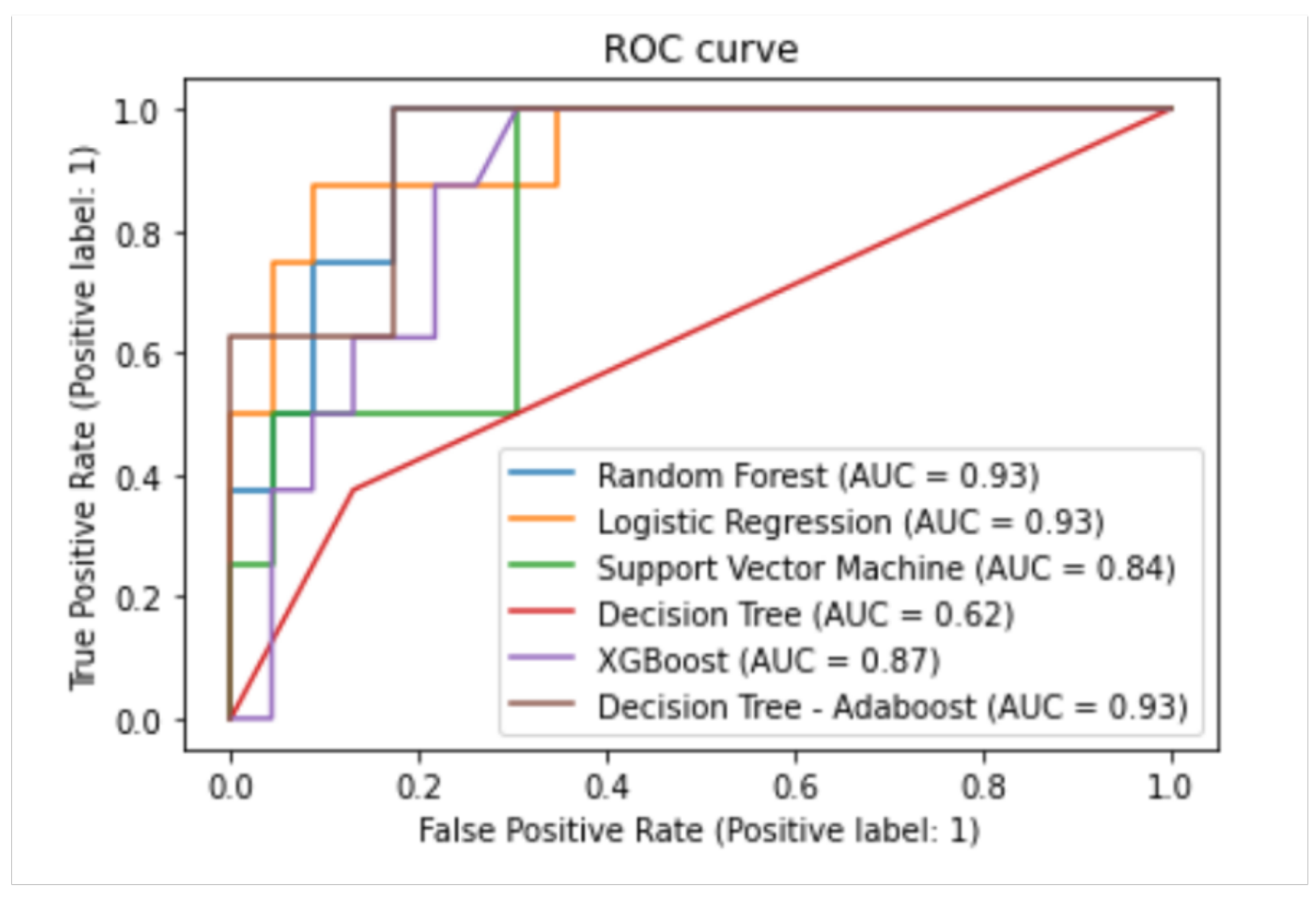
Algorithm	Balanced Accuracy (%)	Specificity (%)	Sensitivity (%)	AUC (%)
Decision Tree	73	80	66	62
Logistic Regression	82	89	74	93
Support Vector Machine	73	67	80	84
Random Forest	86	90	82	93
Adaboost	92	91	93	93
XGBoost	90	92	88	87

and were obtained using the 10-fold cross-validation procedure. Meanwhile, the hyperparameters of the classifiers were tuned to ensure optimal performance. Furthermore, the min–max normalization technique, discussed in Section 2.2, was used to preprocess the data.

According to the balanced accuracy, sensitivity, and specificity values shown in Table 2, the Adaboost classifier achieved the best classification performance with a balanced accuracy, specificity, and sensitivity of 92%, 91%, and 93%, respectively. Meanwhile, both the decision tree and SVM obtained balanced accuracy of 73%, thereby having the least performance. Moreover, from the results, it can be observed that the ensemble classifiers achieved better performance than the conventional classifiers, with the Adaboost achieving the best-balanced accuracy, followed by XGBoost and Random forest. These performances can be attributed to their robust learning process, which involves building multiple base models and the application of a combination rule, such as majority voting, to make the final prediction. Furthermore, Figure 1 shows the various classifiers’ ROC curves and AUC values.

The ROC curve shows the trade-off between sensitivity and specificity. The more the models get closer to the top-left corner, the better the model is at detecting the positive and negative classes in the data. In contrast, models with a ROC curve close to the diagonal line indicate a model that randomly predicts the class. From the ROC curves, the Adaboost achieved a better AUC than the other models, as depicted in Figure 1. The AUC quantifies the ROC curve and indicates the size of the plot that is located under the curve. Therefore, models with an AUC closer to 1 are usually preferred, implying that they can distinguish between the positive and negative classes. The AUC of the Random Forest, Logistic Regression, and AdaBoost were better at 0.93 over the XGBoost, Support Vector Machine, and Decision Tree at 0.87, 0.84, and 0.62, respectively.

4. Interpretability

The ability to understand how a model predicted an outcome is extremely important. Since it was crucial to select features that were useful for the model to make predicted outcomes, we used the decision tree algorithm for this task. The Adaboost algorithm was used in SHAP because the model recorded the highest performance in terms of balanced accuracy of 93%. The SHAP values were derived from the training data, which are used to deduce how a model learned a mapping of features to a prediction.

For our work, the model explanation shows how some features contribute to pushing the model output from the “base” value to the predicted value for the first prediction. The base value is the average of the outcome variable in the training set. The higher value of 1 is an indication that a patient died from hepatitis B, with features such as Albumin, Sgot, Age, Histology, and Bilirubin levels indicating a strong likelihood. It is important to note that red shows a higher value in the prediction, and blue is an indication of a lower value. An example of SHAP values for four instances is presented in Figure 2. A more similar density scatter plot is presented in Figure 3.

In Figure 3, the feature is determined on the y-axis, and the SHAP values are presented on the x-axis. Colors are representations of the values of the features from low to high. Here, as the intensity of the red color increases, the value of the features increases. Conversely, as the intensity of the blue color increases, the value of the features decreases. We can see that Bilirubin has the greatest variability in SHAP values. A high Bilirubin level positively contributes to a high mortality rate. This is closely followed by high ascites levels. Age is another interesting feature. It should be noted that older patients are more likely to die when they have high levels of bilirubin, ascites, alkaline, and malaise levels. Gender has the opposite impact. Hepatitis B can affect any gender, which may not necessarily contribute to higher mortality rates. This is followed by fatigued, spleenP, anorexia, and liverF levels.

5. Discussion

A great deal of improvements has been made in diagnosing, detecting, and preventing hepatitis B. From clinical, statistical, and machine learning, these improvements focus on providing a lasting solution to the menace of HBV. Differentiating hepatitis B from hepatitis caused by other viral agents may not be clinically possible except through laboratory confirmation of the diagnosis.

Different biochemical and virological factors can be used to identify liver damage and viral activity in a patient infected with hepatitis B [12]. This diagnosis can differentiate between acute and chronic hepatitis B infections. However, research has shown that statistical methods can predict acute and chronic HBV using clinical data. For instance, in Jinjin et al. [73], clinical data of 1373 patients with acute deterioration of HBV chronic liver disease were used to identify the clinical characteristics of HBV. The statistical model produces a prognostic score for the onset of Acute-on-chronic liver failure. Jinjin et al. [73] suggest that statistical methods can accurately predict HBV-related chronic liver disease and can be used as a guide for clinical management [73]. Similarly, with the hepatitis B dataset, we used machine learning algorithms, such as decision trees, logistic regression, SVM, random forest, XGBoost, and AdaBoost, to identify patterns and features that show unique relationships between covariates. Our result corroborates with the work in [74] that indicates that machine learning can identify and predict the risk of HBV.

Unlike other studies that use machine learning to diagnose HBV, such as [74,75,76], the decision tree classifier identified bilirubin as having the highest variability in SHAP values (see Figure 1). Since bilirubin is produced from the breakdown of red blood cells in the human body. A higher bilirubin level suggests liver disease or damage, indicating the presence of HBV or other problems. The interpretation of the machine learning model increases the model’s efficacy transparency and promotes increased confidence in the approach, especially for the medical practitioner or health policy maker. In addition to the bilirubin identified by the decision tree model, other features contributing to HBV death include high ascites levels, age, alkaline, and malaise levels, as summarised in Figure 2. Such information can be helpful to health practitioners or health policymakers in making decisions at a glance from the visualized model interpretation summary.

A similar study in [77] used the CRISP-ML method to determine the interpretability level required by stakeholders for a successful real-world solution. CRISP-ML approach differs from our study because it was used to develop an interpretation requirement for data diversity problems and to manage the unstructured nature of data in the healthcare domain. Similarly, we compared our work with the state-of-the-art machine learning models used for hepatitis B predictability, as summarized in

Table 3. Comparison with other studies.

Reference	Method	Model Explainability
Tian et al. [25]	XGBoost, LR, RF and DCT	✗
Khan et al. [79]	SVM	✗
Vijayalakshmi et al. [80]	SGD	✗
Kamimura et al. [28]	DNN	✗
Putri et al. [27]	RF, NB	✗
Chen et al. [81]	RF	✗
Bar-lev et al. [82]	LR, RF and NN	✗
Wu et al. [83]	CNN	✗
Wübbolding et al. [26]	LR, SVM and SGD	✗
Kim et al. [78]	GBM	✓
Xia et al. [29]	LSTM, RNN and BPNN	✗
Wei et al. [84]	DCT, RF and GB	✗
Alamsyah and Fadila [85]	SVM	✗
Our work	RF, LR, SVM, DCT, AdaBoost, and XGBoost	✓

. Of the studies reviewed, only the work of Kim et al. [78] considered model explainability to the Gradient Boosting Machine (GBM) algorithm. The remaining studies never considered this option.

The more the feature of a dataset increases, the better the performance of the model. One major limitation of this study is the lack of available large data size for hepatitis B. However, our study focused more on the interpretability of the model. In the future, we recommend an increased clinical dataset size for hepatitis B to assist in improving the performance of the machine learning model, especially during the model training time.

6. Conclusions

This study used demographic and clinical records of patients obtained from the UCI Machine Learning Repository and applied the SHAP interpretable machine learning approach to predict hepatitis B. AdaBoost achieved an accuracy score of 92%, among other models. We used the AdaBoost classifier for model explainability, and it showed that bilirubin was the most significant feature. This result indicated that a high bilirubin level positively contributed to a high mortality rate. Furthermore, our model showed that older patients are more likely to die when they have high bilirubin levels. Conversely, the gender variable had the opposite impact. Hepatitis B can affect any gender, but it may not necessarily contribute to higher mortality rates. Our study can be helpful for health practitioners and health policymakers in explaining the result of machine learning models to solve health-related problems.

References

- Hepatitis B Foundation: Hepatitis B Facts and Figures. 2019. Available online: https://deepai.org/machine-learning-glossary-and-terms/neural-network (accessed on 25 May 2022).
- Brouwer, W.; Chan, H.; Brunetto, M.; Martinot-Peignoux, M.; Arends, P.; Cornberg, M.; Cherubini, B.; Thompson, A.; Liaw, Y.; Marcellin, P.; et al. Good Practice in using HBsAg in Chronic Hepatitis B Study Group (GPs-CHB Study Group). Repeated Measurements of Hepatitis B Surface Antigen Identify Carriers of Inactive HBV During Long-term Follow-up. Clin. Gastroenterol. Hepatol. 2016, 10, 1481–1489. [Google Scholar] [CrossRef] [Green Version]
- WHO Fact Sheet: Hepatitis B—Symptoms. 2020. Available online: https://www.who.int/news-room/fact-sheets/detail/hepatitis-b (accessed on 30 April 2022).
- Mayo Clinic: Hepatitis B—Symptoms. 2020. Available online: https://shorturl.at/nuzV7 (accessed on 30 April 2022).
- Shu, S.; William, C.W.; Zhuoru, Z.; Dan, D.C.; Jason, J.O.; Polin, C.; Fanpu, J.; Man-Fung, Y.; Guihua, Z.; Wai-Kay, S.; et al. Cost-effectiveness of universal screening for chronic hepatitis B virus infection in China: An economic evaluation. Lancet Glob. Health 2022, 10, e278–e287. [Google Scholar] [CrossRef]
- Tesfa, T.; Hawulte, B.; Tolera, A.; Abate, D. Hepatitis B virus infection and associated risk factors among medical students in Eastern Ethiopia. PLoS ONE 2021, 16, e0247267. [Google Scholar] [CrossRef]
- Nguyen, M.H.; Wong, G.; Gane, E.; Kao, J.H.; Dusheiko, G. Hepatitis B virus: Advances in prevention, diagnosis, and therapy. Clin. Microbiol. Rev. 2020, 33, e00046-19. [Google Scholar] [CrossRef] [PubMed]
- Hu, J.; Protzer, U.; Siddiqui, A. Revisiting hepatitis B virus: Challenges of curative therapies. J. Virol. 2019, 93, e01032-19. [Google Scholar] [CrossRef] [PubMed] [Green Version]
- Lazarus, J.V.; Block, T.; Bréchot, C.; Kramvis, A.; Miller, V.; Ninburg, M.; Pénicaud, C.; Protzer, U.; Razavi, H.; Thomas, L.A.; et al. The hepatitis B epidemic and the urgent need for cure preparedness. Nat. Rev. Gastroenterol. Hepatol. 2018, 15, 517–518. [Google Scholar] [CrossRef] [PubMed]
- Bartenschlager, R.; Urban, S.; Protzer, U. Towards curative therapy of chronic viral hepatitis. Z. Gastroenterol. 2019, 57, 61–73. [Google Scholar] [CrossRef]
- Chen, Y.; Luo, Y.; Huang, W.; Hu, D.; Zheng, R.Q.; Cong, S.Z.; Meng, F.K.; Yang, H.; Lin, H.J.; Sun, Y.; et al. Machine-learning-based classification of real-time tissue elastography for hepatic fibrosis in patients with chronic hepatitis B. Comput. Biol. Med. 2017, 89, 18–23. [Google Scholar] [CrossRef]
- Tai, W.; He, L.; Zhang, X.; Pu, J.; Voronin, D.; Jiang, S.; Zhou, Y.; Du, L. Characterization of the receptor-binding domain (RBD) of 2019 novel coronavirus: Implication for development of RBD protein as a viral attachment inhibitor and vaccine. Cell. Mol. Immunol. 2020, 17, 613–620. [Google Scholar] [CrossRef] [Green Version]
- Strother, H.W.; David, B.D. Estimation of the probability of an event as a function of several independent variables. Biometrika 1967, 54, 167–179. [Google Scholar]
- Uttreshwar, G.S.; Ghatol, A. Hepatitis B Diagnosis Using Logical Inference And Generalized Regression Neural Networks. In Proceedings of the 2009 IEEE International Advance Computing Conference, Patiala, India, 6–7 March 2009; pp. 1587–1595. [Google Scholar] [CrossRef]
- Wang, H.; Liu, Y.; Huang, W. Random forest and Bayesian prediction for Hepatitis B virus reactivation. In Proceedings of the 2017 13th International Conference on Natural Computation, Fuzzy Systems and Knowledge Discovery (ICNC-FSKD), Guilin, China, 29–31 July 2017; pp. 2060–2064. [Google Scholar] [CrossRef]
- Agbele, K.K.; Oriogun, P.K.; Seluwa, A.G.; Aruleba, K.D. Towards a model for enhancing ICT4 development and information security in healthcare system. In Proceedings of the 2015 IEEE International Symposium on Technology and Society (ISTAS), Dublin, Ireland, 11–12 November 2015; pp. 1–6. [Google Scholar]
- Ho, T.K. Random decision forests. In Proceedings of the 3rd International Conference on Document Analysis and Recognition, Montreal, QC, Canada, 14–16 August 1995; Volume 1, pp. 278–282. [Google Scholar] [CrossRef]
- Aruleba, K.; Obaido, G.; Ogbuokiri, B.; Fadaka, A.O.; Klein, A.; Adekiya, T.A.; Aruleba, R.T. Applications of Computational Methods in Biomedical Breast Cancer Imaging Diagnostics: A Review. J. Imaging 2020, 6, 105. [Google Scholar] [CrossRef]
- Aruleba, R.T.; Adekiya, T.A.; Ayawei, N.; Obaido, G.; Aruleba, K.; Mienye, I.; Aruleba, I.; Ogbuokiri, B. COVID-19 Diagnosis: A Review of Rapid Antigen, RT-PCR and Artificial Intelligence Methods. Bioengineering 2022, 3, 153. [Google Scholar] [CrossRef]
- Mienye, I.D.; Obaido, G.; Aruleba, K.; Dada, O.A. Enhanced Prediction of Chronic Kidney Disease Using Feature Selection and Boosted Classifiers. In International Conference on Intelligent Systems Design and Applications; Springer: Cham, Switzerland, 2022; pp. 527–537. [Google Scholar]
- Xiaolu, T.; Yutian, C.; Yutao, H.; Pi, G.; Mengjie, L.; Wangjian, Z.; Zhicheng, D.; Xiangyong, L.; Yuantao, H. Using Machine Learning Algorithms to Predict Hepatitis B Surface Antigen Seroclearance. Comput. Math. Methods Med. 1967, 2019, 2019. [Google Scholar]
- Akbar, K.W.; Peter, D.R.H. Machine learning in medicine: A primer for physicians. Am. J. Gastroenterol. 2010, 105, 1224–1226. [Google Scholar]
- Rohan, G.; Devesh, S.; Mehar, S.; Swati, T.; Rashmi, K.A.; Pravir, K. Artificial intelligence to deep learning: Machine intelligence approach for drug discovery. Mol. Divers 2021, 25, 1315–1360. [Google Scholar]
- Qing-Hai, Y.; Lun-Xiu, Q.; Marshonna, F.; Ping, H.; Jin, W.K.; Amy, C.P.; Richard, S.; Yan, L.; Ana, I.R.; Yidong, C.; et al. Predicting hepatitis B virus–positive metastatic hepatocellular carcinomas using gene expression profiling and supervised machine learning. Nat. Med. 2003, 9, 416–423. [Google Scholar]
- Tian, X.; Chong, Y.; Huang, Y.; Guo, P.; Li, M.; Zhang, W.; Du, Z.; Li, X.; Hao, Y. Using machine learning algorithms to predict hepatitis B surface antigen seroclearance. Comput. Math. Methods Med. 2019, 2019, 6915850. [Google Scholar] [CrossRef]
- Wübbolding, M.; Lopez Alfonso, J.C.; Lin, C.Y.; Binder, S.; Falk, C.; Debarry, J.; Gineste, P.; Kraft, A.R.; Chien, R.N.; Maasoumy, B.; et al. Pilot study using machine learning to identify immune profiles for the prediction of early virological relapse after stopping nucleos (t) ide analogues in HBeAg-negative CHB. Hepatol. Commun. 2021, 5, 97–111. [Google Scholar] [CrossRef] [PubMed]
- Putri, V.; Masjkur, M.; Suhaeni, C. Performance of SMOTE in a random forest and naive Bayes classifier for imbalanced Hepatitis-B vaccination status. J. Physics: Conf. Ser. 2021, 1863, 012073. [Google Scholar] [CrossRef]
- Kamimura, H.; Nonaka, H.; Mori, M.; Kobayashi, T.; Setsu, T.; Kamimura, K.; Tsuchiya, A.; Terai, S. Use of a Deep Learning Approach for the Sensitive Prediction of Hepatitis B Surface Antigen Levels in Inactive Carrier Patients. J. Clin. Med. 2022, 11, 387. [Google Scholar] [CrossRef]
- Xia, Z.; Qin, L.; Ning, Z.; Zhang, X. Deep learning time series prediction models in surveillance data of hepatitis incidence in China. PLoS ONE 2022, 17, e0265660. [Google Scholar] [CrossRef] [PubMed]
- Dua, D.; Graff, C.; UCI Machine Learning Repository. University of California, Irvine, School of Information and Computer Sciences. 2017. Available online: http://archive.ics.uci.edu/ml (accessed on 1 July 2022).
- Mgboh, U.; Ogbuokiri, B.; Obaido, G.; Aruleba, K. Visual Data Mining: A Comparative Analysis of Selected Datasets. In International Conference on Intelligent Systems Design and Applications; Springer: Cham, Switzerland, 2020; pp. 377–391. [Google Scholar]
- Scheda, R.; Diciotti, S. Explanations of Machine Learning Models in Repeated Nested Cross-Validation: An Application in Age Prediction Using Brain Complexity Features. Appl. Sci. 2022, 12, 6681. [Google Scholar] [CrossRef]
- Parvandeh, S.; Yeh, H.W.; Paulus, M.P.; McKinney, B.A. Consensus features nested cross-validation. Bioinformatics 2020, 36, 3093–3098. [Google Scholar] [CrossRef] [PubMed]
- Jones, I. Research Methods for Sports Studies; Routledge: London, UK, 2014. [Google Scholar]
- Patro, S.; Sahu, K.K. Normalization: A preprocessing stage. arXiv 2015, arXiv:1503.06462. [Google Scholar] [CrossRef]
- Sklearn Pipeline. 2022. Available online: https://scikit-learn.org/stable/modules/generated/sklearn.pipeline.Pipeline.html (accessed on 15 October 2022).
- Sevinç, E. An empowered AdaBoost algorithm implementation: A COVID-19 dataset study. Comput. Ind. Eng. 2022, 165, 107912. [Google Scholar] [CrossRef]
- Ogbuokiri, B.; Ahmadi, A.; Bragazzi, N.L.; Movahedi Nia, Z.; Mellado, B.; Wu, J.; Orbinski, J.; Asgary, A.; Kong, J. Public sentiments toward COVID-19 vaccines in South African cities: An analysis of Twitter posts. Front. Public Health 2022, 10, 987376. [Google Scholar] [CrossRef]
- Mienye, I.D.; Sun, Y.; Wang, Z. Prediction performance of improved decision tree-based algorithms: A review. Procedia Manuf. 2019, 35, 698–703. [Google Scholar] [CrossRef]
- Lee, S.J.; Tseng, C.H.; Yang, H.Y.; Jin, X.; Jiang, Q.; Pu, B.; Hu, W.H.; Liu, D.R.; Huang, Y.; Zhao, N. Random RotBoost: An Ensemble Classification Method Based on Rotation Forest and AdaBoost in Random Subsets and Its Application to Clinical Decision Support. Entropy 2022, 24, 617. [Google Scholar] [CrossRef]
- Wu, Y.; Zhang, Q.; Hu, Y.; Sun-Woo, K.; Zhang, X.; Zhu, H.; Li, S. Novel binary logistic regression model based on feature transformation of XGBoost for type 2 Diabetes Mellitus prediction in healthcare systems. Future Gener. Comput. Syst. 2022, 129, 1–12. [Google Scholar] [CrossRef]
- Ogbuokiri, B.; Ahmadi, A.; Nia, Z.M.; Mellado, B.; Wu, J.; Orbinski, J.; Ali, A.; Jude, K. Vaccine Hesitancy Hotspots in Africa: An Insight from Geotagged Twitter Posts. TechRxiv 2022. [Google Scholar] [CrossRef]
- Bokaba, T.; Doorsamy, W.; Paul, B.S. Comparative study of machine learning classifiers for modelling road traffic accidents. Appl. Sci. 2022, 12, 828. [Google Scholar] [CrossRef]
- Ghosh, M.; Sanyal, G. An ensemble approach to stabilize the features for multi-domain sentiment analysis using supervised machine learning. J. Big Data 2018, 5, 1–25. [Google Scholar] [CrossRef]
- Huang, M.W.; Chen, C.W.; Lin, W.C.; Ke, S.W.; Tsai, C.F. SVM and SVM ensembles in breast cancer prediction. PLoS ONE 2017, 12, e0161501. [Google Scholar] [CrossRef]
- Mienye, I.D.; Sun, Y. A Survey of Ensemble Learning: Concepts, Algorithms, Applications, and Prospects. IEEE Access 2022, 10, 99129–99149. [Google Scholar] [CrossRef]
- Mienye, I.D.; Sun, Y.; Wang, Z. An improved ensemble learning approach for the prediction of heart disease risk. Inform. Med. Unlocked 2020, 20, 100402. [Google Scholar] [CrossRef]
- Schonlau, M.; Zou, R.Y. The random forest algorithm for statistical learning. Stata J. 2020, 20, 3–29. [Google Scholar] [CrossRef]
- Lin, W.; Wu, Z.; Lin, L.; Wen, A.; Li, J. An ensemble random forest algorithm for insurance big data analysis. IEEE Access 2017, 5, 16568–16575. [Google Scholar] [CrossRef]
- Zheng, H.; Yuan, J.; Chen, L. Short-term load forecasting using EMD-LSTM neural networks with a Xgboost algorithm for feature importance evaluation. Energies 2017, 10, 1168. [Google Scholar] [CrossRef] [Green Version]
- He, J.; Hao, Y.; Wang, X. An interpretable aid decision-making model for flag state control ship detention based on SMOTE and XGBoost. J. Mar. Sci. Eng. 2021, 9, 156. [Google Scholar] [CrossRef]
- Cheong, Q.; Au-Yeung, M.; Quon, S.; Concepcion, K.; Kong, J.D. Predictive Modeling of Vaccination Uptake in US Counties: A Machine Learning–Based Approach. J. Med. Internet Res. 2021, 23, e33231. [Google Scholar] [CrossRef]
- Dhaliwal, S. Effective intrusion detection system using XGBoost. Information 2018, 9, 149. [Google Scholar] [CrossRef] [Green Version]
- Li, Y.; Chen, W. A comparative performance assessment of ensemble learning for credit scoring. Mathematics 2020, 8, 1756. [Google Scholar] [CrossRef]
- Zheng, H.; Xiao, F.; Sun, S.; Qin, Y. Brillouin Frequency Shift Extraction Based on AdaBoost Algorithm. Sensors 2022, 22, 3354. [Google Scholar] [CrossRef]
- Huang, X.; Li, Z.; Jin, Y.; Zhang, W. Fair-AdaBoost: Extending AdaBoost method to achieve fair classification. Expert Syst. Appl. 2022, 202, 117240. [Google Scholar] [CrossRef]
- Ding, Y.; Zhu, H.; Chen, R.; Li, R. An Efficient AdaBoost Algorithm with the Multiple Thresholds Classification. Appl. Sci. 2022, 12, 5872. [Google Scholar] [CrossRef]
- Nohara, Y.; Matsumoto, K.; Soejima, H.; Nakashima, N. Explanation of machine learning models using improved Shapley Additive Explanation. In Proceedings of the 10th ACM International Conference on Bioinformatics, Computational Biology and Health Informatics, Niagara Falls, NY, USA, 7–10 September 2019; pp. 546–546. [Google Scholar]
- Mangalathu, S.; Hwang, S.H.; Jeon, J.S. Failure mode and effects analysis of RC members based on machine-learning-based SHapley Additive exPlanations (SHAP) approach. Eng. Struct. 2020, 219, 110927. [Google Scholar] [CrossRef]
- García, M.V.; Aznarte, J.L. Shapley additive explanations for NO2 forecasting. Ecol. Inform. 2020, 56, 101039. [Google Scholar] [CrossRef]
- Strumbelj, E.; Kononenko, I. An efficient explanation of individual classifications using game theory. J. Mach. Learn. Res. 2010, 11, 1–18. [Google Scholar]
- Nohara, Y.; Matsumoto, K.; Soejima, H.; Nakashima, N. Explanation of machine learning models using shapley additive explanation and application for real data in hospital. Comput. Methods Programs Biomed. 2022, 214, 106584. [Google Scholar] [CrossRef]
- Pokharel, S.; Sah, P.; Ganta, D. Improved prediction of total energy consumption and feature analysis in electric vehicles using machine learning and shapley additive explanations method. World Electr. Veh. J. 2021, 12, 94. [Google Scholar] [CrossRef]
- Santos, R.N.; Yamouni, S.; Albiero, B.; Vicente, R.; A Silva, J.; FB Souza, T.; CM Freitas Souza, M.; Lei, Z. Gradient boosting and Shapley additive explanations for fraud detection in electricity distribution grids. Int. Trans. Electr. Energy Syst. 2021, 31, e13046. [Google Scholar] [CrossRef]
- Meddage, P.; Ekanayake, I.; Perera, U.S.; Azamathulla, H.M.; Md Said, M.A.; Rathnayake, U. Interpretation of Machine-Learning-Based (Black-box) Wind Pressure Predictions for Low-Rise Gable-Roofed Buildings Using Shapley Additive Explanations (SHAP). Buildings 2022, 12, 734. [Google Scholar] [CrossRef]
- Pedregosa, F.; Varoquaux, G.; Gramfort, A.; Michel, V.; Thirion, B.; Grisel, O.; Blondel, M.; Prettenhofer, P.; Weiss, R.; Dubourg, V.; et al. Scikit-learn: Machine learning in Python. J. Mach. Learn. Res. 2011, 12, 2825–2830. [Google Scholar]
- Elgeldawi, E.; Sayed, A.; Galal, A.R.; Zaki, A.M. Hyperparameter tuning for machine learning algorithms used for arabic sentiment analysis. Informatics 2021, 8, 79. [Google Scholar] [CrossRef]
- Chicco, D.; Jurman, G. The advantages of the Matthews correlation 609 coefficient (MCC) over F1 score and accuracy in binary classification 610 evaluation. BMC Genom. 2020, 21, 6. [Google Scholar] [CrossRef] [Green Version]
- Mienye, I.D.; Sun, Y. Performance analysis of cost-sensitive learning methods with application to imbalanced medical data. Inform. Med. Unlocked 2021, 25, 100690. [Google Scholar] [CrossRef]
- Trevethan, R. Sensitivity, specificity, and predictive values: Foundations, pliabilities, and pitfalls in research and practice. Front. Public Health 2017, 5, 307. [Google Scholar] [CrossRef]
- Mienye, I.D.; Sun, Y. Improved heart disease prediction using particle swarm optimization based stacked sparse autoencoder. Electronics 2021, 10, 2347. [Google Scholar] [CrossRef]
- Namdar, K.; Haider, M.A.; Khalvati, F. A Modified AUC for Training Convolutional Neural Networks: Taking Confidence into Account. Front. Artif. Intell. 2021, 4, 582928. [Google Scholar] [CrossRef]
- Luo, J.; Liang, X.; Xin, J.; Li, J.; Li, P.; Zhou, Q.; Hao, S.; Zhang, H.; Lu, Y.; Wu, T.; et al. Predicting the Onset of Hepatitis B Virus–Related Acute-on-Chronic Liver Failure. Clin. Gastroenterol. Hepatol. 2022; in press. [Google Scholar] [CrossRef]
- Yarasuri, V.K.; Indukuri, G.K.; Nair, A.K. Prediction of Hepatitis Disease Using Machine Learning Technique. In Proceedings of the 2019 Third International conference on I-SMAC (IoT in Social, Mobile, Analytics and Cloud) (I-SMAC), Palladam, India, 12–14 December 2019; pp. 265–269. [Google Scholar] [CrossRef]
- Fatima, M.; Pasha, M. Survey of Machine Learning Algorithms for Disease Diagnostic. J. Intell. Learn. Syst. Appl. 2017, 9, 16. [Google Scholar] [CrossRef] [Green Version]
- Ali, N.; Srivastava, D.; Tiwari, A.; Pandey, A.; Pandey, A.K.; Sahu, A. Predicting Life Expectancy of Hepatitis B Patients using Machine Learning. In Proceedings of the 2022 IEEE International Conference on Distributed Computing and Electrical Circuits and Electronics (ICDCECE), Ballari, India, 23–24 April 2022; pp. 1–4. [Google Scholar] [CrossRef]
- Kolyshkina, I.; Simoff, S. Interpretability of Machine Learning Solutions in Public Healthcare: The CRISP-ML Approach. Front. Big Data 2021, 4, 660206. [Google Scholar] [CrossRef] [PubMed]
- Kim, H.Y.; Lampertico, P.; Nam, J.Y.; Lee, H.C.; Kim, S.U.; Sinn, D.H.; Seo, Y.S.; Lee, H.A.; Park, S.Y.; Lim, Y.S.; et al. An artificial intelligence model to predict hepatocellular carcinoma risk in Korean and Caucasian patients with chronic hepatitis B. J. Hepatol. 2022, 76, 311–318. [Google Scholar] [CrossRef] [PubMed]
- Khan, S.; Ullah, R.; Khan, A.; Ashraf, R.; Ali, H.; Bilal, M.; Saleem, M. Analysis of hepatitis B virus infection in blood sera using Raman spectroscopy and machine learning. Photodiagn. Photodyn. Ther. 2018, 23, 89–93. [Google Scholar] [CrossRef] [PubMed]
- Vijayalakshmi, C.; Mohideen, S.P. Predicting Hepatitis B to be acute or chronic in an infected person using machine learning algorithm. Adv. Eng. Softw. 2022, 172, 103179. [Google Scholar] [CrossRef]
- Chen, S.; Zhang, Z.; Wang, Y.; Fang, M.; Zhou, J.; Li, Y.; Dai, E.; Feng, Z.; Wang, H.; Yang, Z.; et al. Using quasispecies patterns of hepatitis B virus to predict hepatocellular carcinoma with deep sequencing and machine learning. J. Infect. Dis. 2021, 223, 1887–1896. [Google Scholar] [CrossRef] [PubMed]
- Bar-Lev, S.; Reichman, S.; Barnett-Itzhaki, Z. Prediction of vaccine hesitancy based on social media traffic among Israeli parents using machine learning strategies. Isr. J. Health Policy Res. 2021, 10, 1–8. [Google Scholar] [CrossRef]
- Albogamy, F.R.; Asghar, J.; Subhan, F.; Asghar, M.Z.; Al-Rakhami, M.S.; Khan, A.; Nasir, H.M.; Rahmat, M.K.; Alam, M.M.; Lajis, A.; et al. Decision Support System for Predicting Survivability of Hepatitis Patients. Front. Public Health 2022, 10, 862497. [Google Scholar] [CrossRef]
- Wei, R.; Wang, J.; Wang, X.; Xie, G.; Wang, Y.; Zhang, H.; Peng, C.Y.; Rajani, C.; Kwee, S.; Liu, P.; et al. Clinical prediction of HBV and HCV related hepatic fibrosis using machine learning. EBioMedicine 2018, 35, 124–132. [Google Scholar] [CrossRef] [Green Version]
- Alamsyah, A.; Fadila, T. Increased accuracy of prediction hepatitis disease using the application of principal component analysis on a support vector machine. J. Phys. Conf. Ser. 2021, 1968, 012016. [Google Scholar] [CrossRef]