Article

Building Networks with a New Cross-Bubble Transition Entropy for Quantitative Assessment of Mental Arithmetic Electroencephalogram

1
School of Mechanical Engineering, Xi’an Jiaotong University, Xi’an 710049, China
2
State Key Laboratory for Manufacturing Systems Engineering, Xi’an Jiaotong University, Xi’an 710049, China
*
Author to whom correspondence should be addressed.
Submission received: 20 September 2022 / Revised: 30 October 2022 / Accepted: 2 November 2022 / Published: 3 November 2022
(This article belongs to the Special Issue Advances in Neuroimaging Data Processing)

Abstract

:
The complex network nature of human brains has led an increasing number of researchers to adopt a complex network to assess the cognitive load. The method of constructing complex networks has a direct impact on assessment results. During the process of using the cross-permutation entropy (CPE) method to construct complex networks for cognitive load assessment, it is found that the CPE method has the shortcomings of ignoring the transition relationship between symbols and the analysis results are vulnerable to parameter settings. In order to address this issue, a new method based on the CPE principle is proposed by combining the advantages of the transition networks and the bubble entropy. From an interaction perspective, this method suggested that the node-wise out-link transition entropy of the cross-transition network between two time series is used as the edge weight to build a complex network. The proposed method was tested on the unidirectional coupled Henon model and the results demonstrated its suitability for the analysis of short time series by decreasing the influence of the embedding dimension and improving the reliability under the weak coupling conditions. The proposed method was further tested on the publicly available EEG dataset and showed significant superiority compared with the conventional CPE method.

1. Introduction

Different levels of cognitive demand can accommodate the complexity and variability of the everyday tasks and the environments, and can result in different cognitive loads [1,2,3]. Continuous high cognitive load will not only lead to inefficient work but also accidents that might lead to life-threatening consequences. In addition, it also has negative effects on physical and mental health, such as insomnia, decreased immunity, susceptibility to infection, and migraines [4,5,6,7,8]. As a practical necessity, the evaluation of cognitive load or mental load has become a hot topic of research. Therefore, it is of practical significance to design and build a system capable of detecting cognitive load. The use of such a system will not only make it possible to assess the impact of different tasks on the cognitive load, but more importantly, a timely and accurate estimate of cognitive load will help to determine the optimum level of mental load, in order to prevent accidents and make workers more compatible with the work environment. Conventionally, the measurement of cognitive load can be divided into subjective and objective measures [9]. Subjective measures are collected via interviews or questionnaires. They are usually unreliable due to the subjective opinions of the participants [10,11,12]. In contrast, objective measures that are mainly based on task performances or derived from physiological recordings are less intrusive to the task and independent of the participants’ opinion. With the development of technology, neurophysiological activities from brain, heart, and eye movement can be recorded and analyzed to reflect the mental state objectively in a noninvasive way [13]. Previous studies have confirmed that signals such as near-infrared spectroscopy (NIRS), functional magnetic resonance imaging (fMRI), electrocorticography (ECoG), or electroencephalography (EEG) are closely correlated with brain status and can provide a useful way to assess cognitive load [14,15,16,17,18]. Among these physiological signals, EEG has been widely concerned by researchers because of its high time resolution, noninvasiveness, convenience, security, cheapness, and portability [19,20].
In general, the EEG signal is nonstationary and nonlinear. Linear analysis techniques in the time–frequency domain can be used to detect rhythmic oscillations, but the contained nonlinear information cannot be effectively extracted [21]. Therefore, many scholars have attempted to extract various nonlinear parameters from EEG signals and combine them with the machine learning technique in order to effectively capture the subtle information related to the physiological states. Nilima Salankar et al. used the empirical mode decomposition (EMD) and the variational mode decomposition (VMD) to decompose the EEG signals, respectively, and then used the second-order difference plots for feature mining of the decomposed intrinsic modes. The results showed that alcoholic (A) and nonalcoholic (NA) subjects could be accurately classified when using short-duration EEG recordings [22]. Mohammad Shahbakhti et al. proposed extracting Katz and Higuchi’s fractal dimensions, dispersion entropy, and bubble entropy from the sub-band of a single-channel frontal EEG recording to construct the nonlinear feature set and then differentiate between the arousal and the sleep stage I [23]. Jose Kunnel Paul et al. used seven nonlinear parameters, including the sample entropy (SampEn), fractal dimension (FD), higher-order spectrum (HOS), maximum Lyapunov index (LLE), Kolmogorov complexity (KC), Hurst index (HE), and the band power of the EEG signal in sleep stage 2 and 3 as the features to classify between patients with fibromyalgia and healthy controls. The accuracy, sensitivity, and specificity of the classification results were 96.15%, 96.88%, and 95.65%, respectively [24]. The nonlinear parameters in the above-mentioned methods were taken from individual EEG channels and involve no information on the interaction between different channels. However, previous research has shown that the brain should be treated as a complex network system based on the many features it shares with networks of other biological and physical systems [25]. Complex network analysis is a powerful technique based on the graph theory that typically uses a small number of valid and reliable measures to capture the features of the brain network [26]. There is a growing interest in the cognitive load assessment through the construction of complex networks, and various methods have been proposed to convert time series into networks [27,28,29,30]. Complex networks constructed using different network construction algorithms may have distinct, significantly different properties [31]. A variety of methods have been proposed so far to define the concept of connectivity between nonlinearly coupling components and investigate the characteristics of the topological properties of networks. Among different methods, for example, the mutual information (MI) (including its time-delayed version) [32,33], transfer entropy (TE) [34], inner composition alignment (IOTA) [35] and cross-sample entropy (CSE) [36], the TE is widely used in particular as a nonparametric measure that does not rely on any assumption of some model and can capture the directional and dynamic interaction between the different components of a time series [37,38]. However, in practice, an unavoidable pitfall of TE is that robust estimation of the interactions requires long-term data recordings. In order to meet the need for interaction estimation using finite data samples, Shi et al. proposed the CPE by fusing inner composition alignment (IOTA) and permutation entropy, and validated it in financial time series analysis [39], noting that CPE was simple, stable, and efficient.
In the original CPE method, only the probability distribution of the symbols after coarse graining of the affected time series is considered during the calculation of entropy, ignoring the transition relationship between the symbols in the temporal domain. For example, given the symbolized set A = [2 2 4 3 5 1 2] and B = [1 2 2 5 3 2 4 ], the probability distributions of the elements in set A and set B are the same and, therefore, the original CPE method would obtain the same entropy value. In addition, like other nonlinear measures, the CPE method involves the manual selection of parameters to ensure the effectiveness of the results. In order to address these issues, a new method to construct the complex network based on the cross-transition network was proposed in this study to assess cognitive load. The novelty of the method lies in incorporating the advantages of transition network and bubble entropy [40] into the CPE to estimate the coupling strength of two time series from a cross-network perspective. The node-wise out-link transition entropy of two time series cross-transition networks was proposed as the edge weights between two time series to construct the complex network, and the network parameters were extracted as a quantitative measurement of the cognitive load. Referring to the symbolization process of the bubble entropy, the number of swaps required to sort the phase space reconstruction vectors of the affected time series in the ascending order was used instead of the number of intersections calculated by the OITA method in the original CPE. In order to verify the effectiveness of the proposed method, the unidirectional coupled Honen model with different coupling strengths was used, and the results were compared with those obtained using the original CPE. The proposed method and the original CPE method were further compared by constructing the complex network on the realistic EEG recordings from the mental arithmetic task. The significance of the selected network indicator and the capability of the proposed method to differentiate different levels of brain cognitive load were verified using the nonparametric permutation test.
The contributions of this paper are as follows.
1. Based on the cross-transition network, a novel method is proposed that reflects the information interaction between two time series in more detail.
2. The symbolization process with reference to the bubble entropy minimizes the effect of parameter setting on the analysis results.
3. The topological characteristics of complex networks constructed using the node-wise out-link transition entropy of cross-transition networks as the edge weights have the potential to provide useful indicators for physiological complex networks.
This paper is organized as follows. In Section 2, the implementation process of the proposed method in this study is described in detail. In Section 3, the CPE and the proposed method are used to analyze the unidirectional coupled Honen model with its parameters varied, respectively, and their performance is compared. Next, a realistic EEG dataset recorded during the mental arithmetic task is analyzed by constructing the complex networks using the two methods, respectively, in order to further demonstrate the effectiveness of the proposed method. The discussion and conclusions are given in Section 4 and Section 5.

2. Materials and Methods

In this section, the CPE method is briefly introduced, and then the detailed implementation process of the proposed method is described.

2.1. CPE

Based on the permutation entropy and IOTA, Shi et al. proposed the CPE to analyze the information interactions between financial time series [39]. The implementation process is as follows:
  • For two time series with the same length { x ( t ) } and { y ( t ) } , t = [ 1 , 2 , , N ] , their state vectors X t = [ x t , x t + τ , x t + 2 τ , , x t + ( d 1 ) τ ] and Y t = [ y t , y t + τ , y t + 2 τ , , y t + ( d 1 ) τ ] , t [ 1 , 2 , N ( d 1 ) τ ] , are obtained through the phase space reconstruction procedure using the delay parameter τ and the embedding dimension d .
  • Performing nondecreasing sort on state vector X t , and obtaining its position index π X . Rearranging the state vector Y t with the position index π X as the standard, and the result is recorded as G t = Y t ( π x ) .
  • Based on the principle of IOTA, the monotonicity is quantified by counting the number of intersection points of the horizontal lines which are drawn from each data point of G t and G t itself. The intersections number of the kth state vector is calculated using the following equation:
k t = i = 1 d 2 j = i + 1 d 1 Θ [ ( G t ( j + 1 ) G t ( i ) ) ( G t ( i ) G t ( j ) ) ]
where Θ [ x ] is the Heaviside function:
Θ [ x ] = { 1 ,   x > 0 0 ,   x 0
4.
According to this method, all state vectors of the time series are traversed, and the number of the intersections of each state vector can be expressed as a unique integer z , z [ 0 , R ] , R = ( d 1 ) ( d 2 ) / 2 is the maximum possible number of intersections. For all the R + 1 possible values for the integer z i , i = 0 , 1 , , R of intersection points k t in each state vectors, its probability can be obtained by
p ( z i ) = # { k t | k t = z i } N ( d 1 ) τ
where 1 t N ( d 1 ) τ , 0 i R , # is the number of elements in the set. Then, after obtaining the probability distribution set P = { p ( z i ) , i = 1 , , R } , CPE is defined as:
H x y ( d , τ ) = i = 0 R p ( z i ) log 2 p ( z i )
According to the above definition, the greater the coupling strength between the two time series, the smaller the CPE. For two random time series, the entropy value reaches the theoretical maximum log 2 ( R + 1 ) .

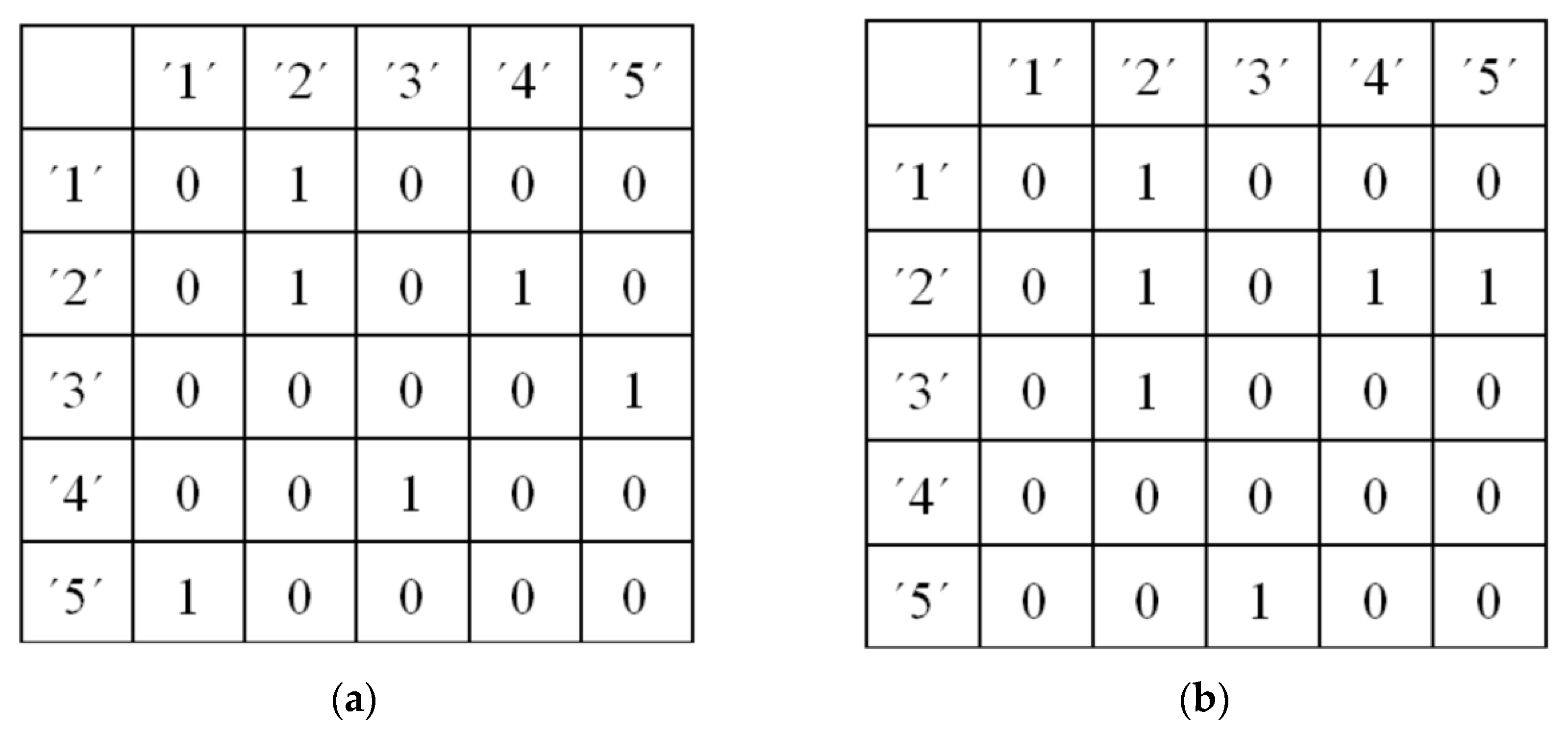
2.2. Cross-Bubble Transition Network (CBTN)

In the original CPE, the process of counting the intersection number of each state vector is essentially a symbolization of it. In the calculation of entropy, only the probability distribution of symbols is considered and the transition behavior between adjacent symbols is ignored. Therefore, the transition network is introduced, in which each symbol is taken as a node and a directional weighted complex network is constructed based on the temporal adjacency of the symbols, with the network weights being the number of transitions between nodes. In addition, to limit the impact of parameter selection on the analysis results, the symbolization process of the bubble entropy was referenced by replacing the intersection number corresponding to each state vector with the number of swaps necessary to sort the state vector in ascending order. The specific implementation process of the cross-bubble transition entropy (Algorithm 1) is as follows:
  • For two equal length time series { x ( t ) } and { y ( t ) } , t = [ 1 , 2 , , N ] , their state vectors X t = [ x t , x t + τ , x t + 2 τ , , x t + ( d 1 ) τ ] and Y t = [ y t , y t + τ , y t + 2 τ , , y t + ( d 1 ) τ ] , t [ 1 , 2 , , N ( d 1 ) τ ] , are obtained through the phase space reconstruction procedure using the delay parameter τ and the embedding dimension d . Here, following the parameter choice of bubble entropy, τ = 1 ;
  • Performing ascending sort on the state vector X t , and obtaining its position index π X t . The state vector Y t was rearranged using the position index π X t as a criterion and the result was recorded as G t = Y t ( π X t ) , t [ 1 , 2 , , N d + 1 ] ;
  • Sorting the elements in each state vector G t = Y t ( π X t ) , t [ 1 , 2 , , N d + 1 ] in ascending order, and calculating the necessary number of swaps S i , S i [ 0 , 1 , , d ( d 1 ) / 2 ] ; this is because the number of possible swaps in bubble sort for a d dimensional state vector is from 0 to d ( d 1 ) / 2 ;
  • Using S i , S i [ 0 , 1 , , d ( d 1 ) / 2 ] as network nodes, a directional weighted complex network W was constructed according to the temporal adjacency relationship of S i and the weight of the network W was the numbers of transition between nodes;
  • In order to reflect the connection relationship between nodes as much as possible, the node-wise out-link transition entropy (NOTE) of the adjacency matrix W was proposed to be used as an indicator parameter. The NOTE was obtained as follows.
The Shannon entropy of each row of the adjacency matrix W was calculated to obtain the local node out-link entropy S W i , which was used to measure the probability distribution of the output strengths of each node.
S W i = j = 0 ; j i D w i j log 2 ( w i j )
where D = d ( d 1 ) / 2 , w i j was the ratio of the output strength from node i to node j to all the output strengths of node i , j = 0 D w i j = 1 , and the normalized S W i was
H W i = S W i / S i , max
where S i , max = log 2 ( D + 1 ) was the normalization factor and kept the same for all nodes.
The node-wise out-link transition entropy of the adjacency matrix W was
H N O T E = i = 0 D p i H W i
where p i was the probability distribution of each node.
The pseudo-code of the proposed algorithm is illustrated as follows.
Algorithm 1. Cross-bubble transition entropy
CBTN ( x ( t ) , y ( t ) , d , τ )        // x ( t ) , y ( t ) are time series. d is embedding dimensions. τ is delay time.
1    performing phase space reconstruction on x ( t ) , y ( t ) to get
   X t = [ x t , x t + τ , x t + 2 τ , , x t + ( d 1 ) τ ] and Y t = [ y t , y t + τ , y t + 2 τ , , y t + ( d 1 ) τ ] , t [ 1 , 2 , , N ( d 1 ) τ ]
2    for t = 1   to   N ( d 1 ) τ
3    performing ascending sort on X t to get its position index π X t ,
4     Y t is rearranged according to π X t to get G t = Y t ( π X t ) ,
5     sorting G t in ascending order by bubble method and get swaps number S i ,
S i [ 0 , 1 , , d ( d 1 ) / 2 ] .     // d ( d 1 ) / 2 is the maximum swaps number
6    Using S i as network nodes,   by   temporal   adjacency   relationship   of   S i to construct a directed weighted complex network W .
7    for i = 0 to D         // D = d ( d 1 ) / 2
8     S W i = j = 0 ; j i D w i j log 2 ( w i j ) ,    // j = 0 D w i j = 1
9    normalizing S W i to get H W i = S W i / S i , max ,   // S i , max = log 2 ( D + 1 )
10   H N O T E = 0 .
11   for i = 0 to D            // D = d ( d 1 ) / 2
12    H N O T E = H N O T E + p i H W i .    // p i is the probability distribution of S i .
13   return H N O T E .
To demonstrate the performance of the NOTE to track the deterministic dynamical variation in time series, the values with the NOTE and the original CPE were obtained separately for the symbolized sets A = [2 2 4 3 5 1 2] and B = [1 2 2 5 3 2 4 ]. The probability distributions of the elements in the sets A and B were the same. The probability of individual elements sorted in an ascending order were [0.143, 0.428, 0.143, 0.143, 0.143]. The original CPE method would yield an entropy value of 2.128 for both sets. The directional weighted adjacency matrices constructed for the elements in sets A and B according to their temporal adjacency relationship are shown in Figure 1a,b, respectively. The two adjacency matrices exhibited distinct differences. The NOTE value of these two adjacency matrices was 0.1846 and 0.2925, respectively, which shows the different dynamical variations contained in the sets A and B.

3. Analysis and Results

In this section, in order to verify whether the CBTN can characterize the information interaction between two time series, it was first tested on the unidirectional coupled Honen model and its performance was compared with the original CPE method. Next, the complex network constructed by the CBTN was applied to the realistic EEG recordings during either the resting state or the mental arithmetic task in order to evaluate the performance of the proposed method in detecting the changes in the cognitive load.

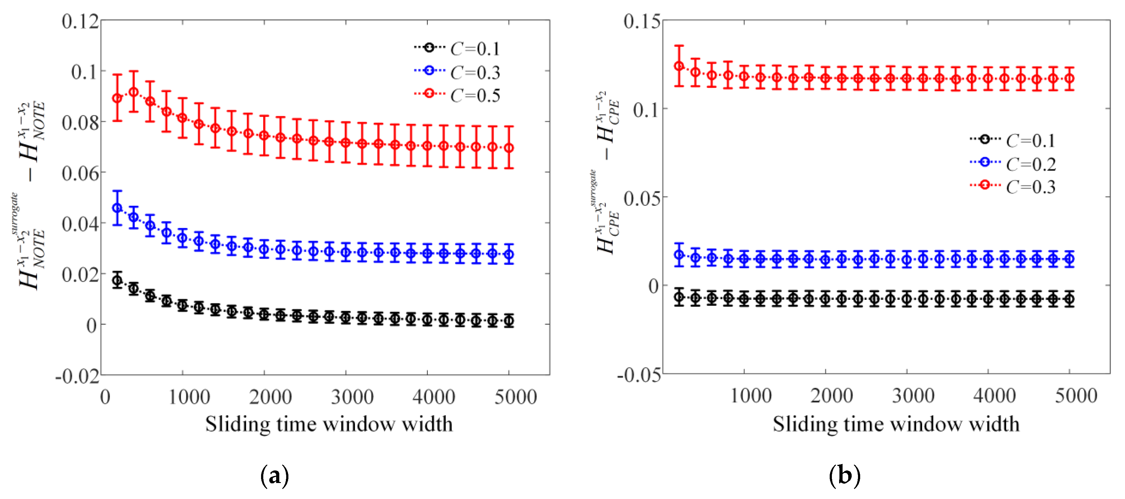
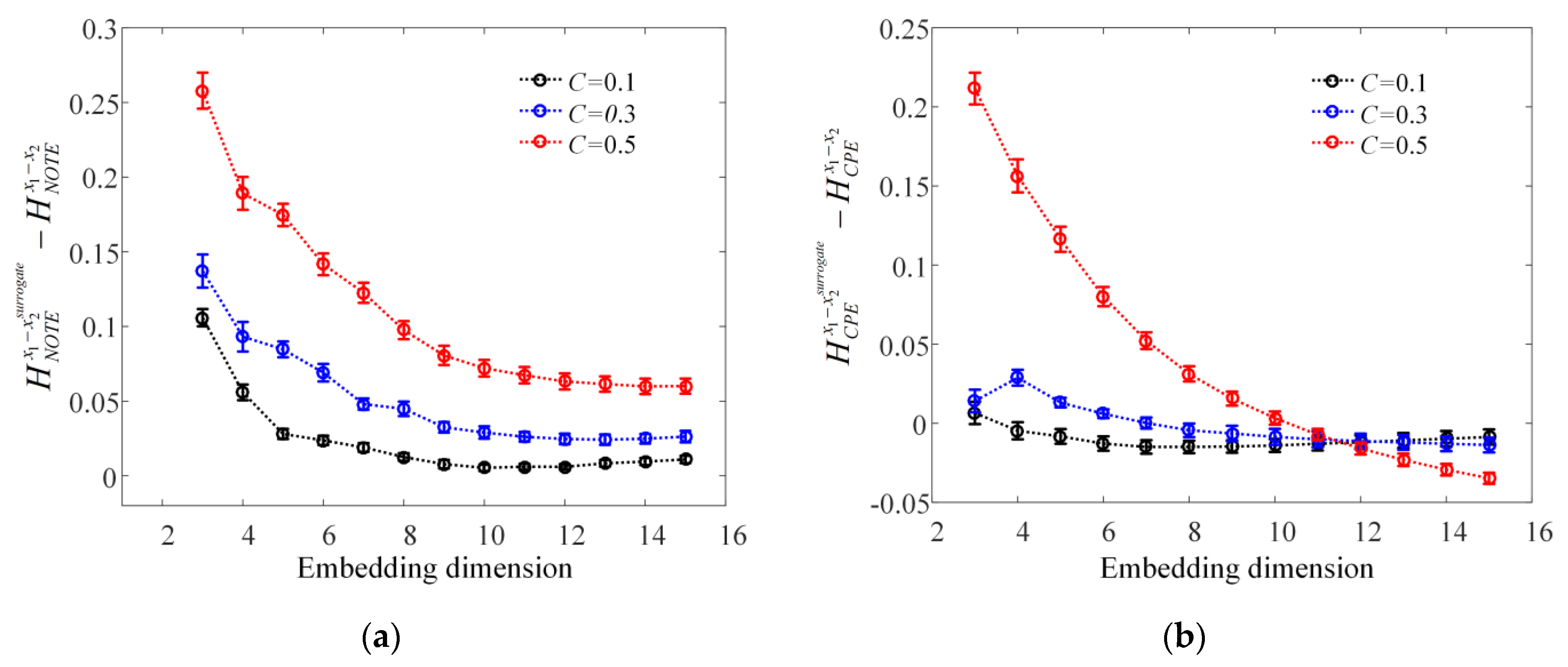
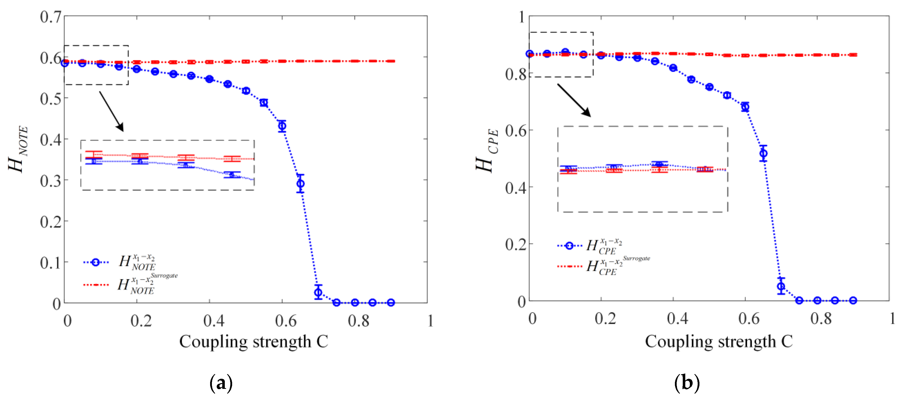
3.1. Analysis of Coupled Dynamic Model

The validity of the proposed method was first tested on signals generated using two Henon map unidirectional coupled subsystems with one as the driver subsystem 1 and the other as the responder subsystem 2. The equations of the system are expressed as follows:
{ x 1 t + 1 = 1.4 x 1 t 2 + 0.3 × y 1 t y 1 t + 1 = x 1 t x 2 t + 1 = 1.4 ( C × x 1 t + ( 1 C ) × x 2 t ) × x 2 t + 0.3 × y 2 t y 2 t + 1 = x 2 t
The parameter C is a coupling parameter varying from 0 to 1. When C is 0, the two subsystems are entirely independent and there is no definite dynamical behavior between them. When C is 1, the two subsystems are completely synchronized and there is a definite dynamical relationship between them. The values of x 1 1 , y 1 1 , x 2 1 and y 2 1 are initialized randomly in the range from 0 to 1. Then, 50,000 points are calculated according to (8) and the first 20,000 are discarded as the transients.
From the definition of CBTN, we can see that the unique parameter relevant to the CBTN is the embedding dimension d . The parameter d defines the embedding spatial dimension of a given time series. Another noteworthy issue is the appropriate signal length in order to obtain reliable results. One fact is that the signal length is limited, and the other is that the calculation process can only be performed in one window. The values of these two parameters determine whether the results of the analysis can be described or not and whether it is possible to extract the deep relationships hidden between the two time series. Here, the determination process of these two parameters is explained by analyzing the unidirectional coupled Honen model with the deterministic coupling relationship. It was selected because the theoretical value of each expected return can be calculated. Based on this theoretical value, it can be evaluated whether the result obtained with a specific parameter setting can converge reliably and stably to the expected value or not. In addition, in order to highlight the impact of the CBTN on the analysis result, the CPE results for the same objects were used as a comparison. When the CPE was used, the embedded dimension was 5 and the delay time was 2.
The appropriate signal length was determined by investigating the effect of the width of the analysis window on the results. For the time series x 1 and x 2 obtained using the unidirectional coupled Henon model under a certain coupling strength, the surrogate data x 2 S u r r o g a t e were first calculated by surrogating x 2 using iAAFT (iterative amplitude-adjusted Fourier transform with five iterations) to mimic the random coupling state. Next, the sliding time window with a fixed moving step of 500 samples was chosen to segment the paired time series x 1 and x 2 and x 1 and x 2 S u r r o g a t e . The purpose of using the sliding time window is to enhance the effect of data analysis. The width of the sliding window width was increased from 200 to 5000 samples with a step of 200 samples. With each window width, the coupling strength between x 1 and x 2 S u r r o g a t e and between x 1 and x 2 was calculated using the CBTN for individual sliding windows, obtaining the H N O T E x 1 x 2 S u r r o g a t e and H N O T E x 1 x 2 , respectively. The differences H N O T E x 1 x 2 S u r r o g a t e H N O T E x 1 x 2 were first calculated for individual windows and then averaged across windows as the measured difference. The same procedure was repeated for 30 times with each window width and then averaged across repetitions to obtain the average and standard deviation of the measured difference. The coupling strength between x 1 and x 2 was set to 0.1, 0.3, and 0.5, respectively, and the results are shown in Figure 2. Figure 2a shows the results of the CBTN method and Figure 2b shows the results of the CPE method. It can be found that the two methods can make a good distinction between different coupling strengths. The CPE method can reach a stable state when the window width is less than 1000 samples, and the CBTN method can reach a stable state when the window width is more than 2000 samples. It was speculated that the CPE was appropriate for the analysis of short time series when it was proposed. Therefore, the appropriate window width for the CBTN is 2000 samples. It should be noted that the differences H C P E x 1 x 2 S u r r o g a t e H C P E x 1 x 2 had a negative value with the CPE method when the coupling strength was 0.1. This is inconsistent with the theory and indicates that the CPE was not capable of differentiating the weak coupling state.
With the determined window width of 2000 samples, the impact of the embedding dimension d on the estimation of the coupling strength was further investigated using the same method as above. The dimension d varied from 3 to 15 with a step of 1. Figure 3 compares the results between the CBTN method and the CPE method. It can be seen that the results of CBTN method tended to be stable with the increase in the embedding dimension d . When the embedding dimension was greater than 10, the measured difference under three coupling strength levels basically reached a stable state. In contrast, the measured difference using the CPE method was greatly affected by the embedded dimension. Within the varying range of the embedded dimension, the measured difference under three coupling strength levels could reach a stable state. When the embedding dimension was greater than 11, the measured difference under the stronger coupling strength (C = 0.3) was even smaller than that under the weaker coupling strength (C = 0.1 and C = 0.2). These results demonstrated that the CBTN method can be less affected by the embedding dimension d compared with the CPE method. More specifically, the embedding dimension would have little influence when it is greater than a certain value. Accordingly, for the unidirectional coupled Henon model, the recommended embedding dimension d for the CBTN method was set to 10.
After the embedding dimension and the sliding window width were determined, the CBTN was used to analyze the unidirectional coupled Honen model under different coupling strengths C . Specifically, the coupling strength C increased from 0 to 0.9 with a step of 0.05. For a given coupling strength, the data of x 1 , x 2 and x 2 S u r r o g a t e within individual sliding windows were analyzed using the CBTN and CPE methods, respectively, to obtain the H N O T E x 1 x 2 , H C P E x 1 x 2 , H N O T E x 1 x 2 S u r r o g a t e and H C P E x 1 x 2 S u r r o g a t e . The procedure was also repeated 30 times under each coupling strength, and the mean value and the standard deviation across 30 repetitions were calculated. Figure 4 illustrates the average value of H N O T E x 1 x 2 , H C P E x 1 x 2 , H N O T E x 1 x 2 S u r r o g a t e and H C P E x 1 x 2 S u r r o g a t e across all repetitions under different coupling strength levels. In the figure, the dashed boxes indicated by the arrows are partial zooms of the analysis results. As can be seen from Figure 4, the greatest difference between the analytical results of CBTN and CPE was mainly in the part where the coupling strength was less than 0.2. In this part, the CBTN method gives correct analysis results, while the CPE calculation results are greater than the values under the random coupling state, which is inconsistent with the theory. The possible reason is the CPE method that is based on the probability distribution statistics of symbols cannot distinguish the interactions between time series under weak coupling conditions. In contrast, the proposed CBTN method has good detection capability of interactions between time series with a weak coupling strength.

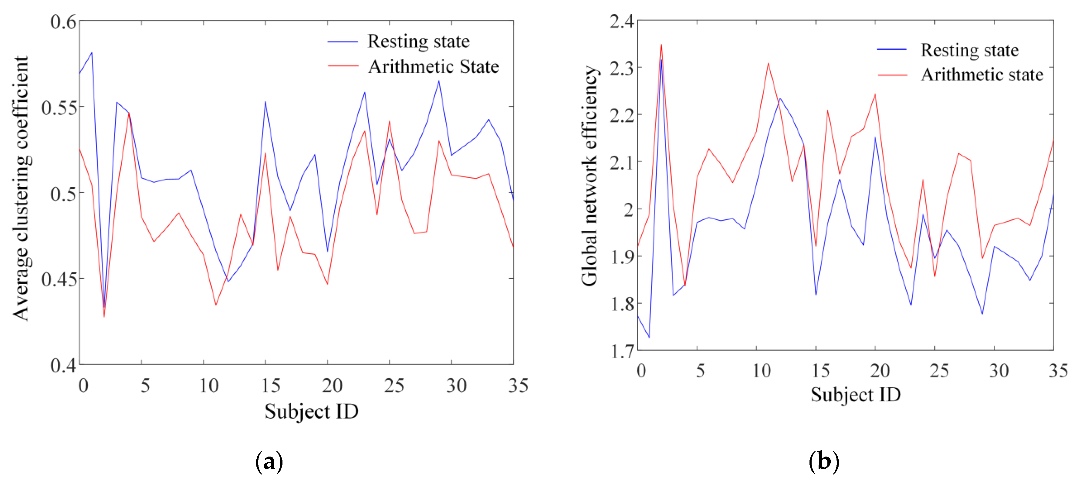
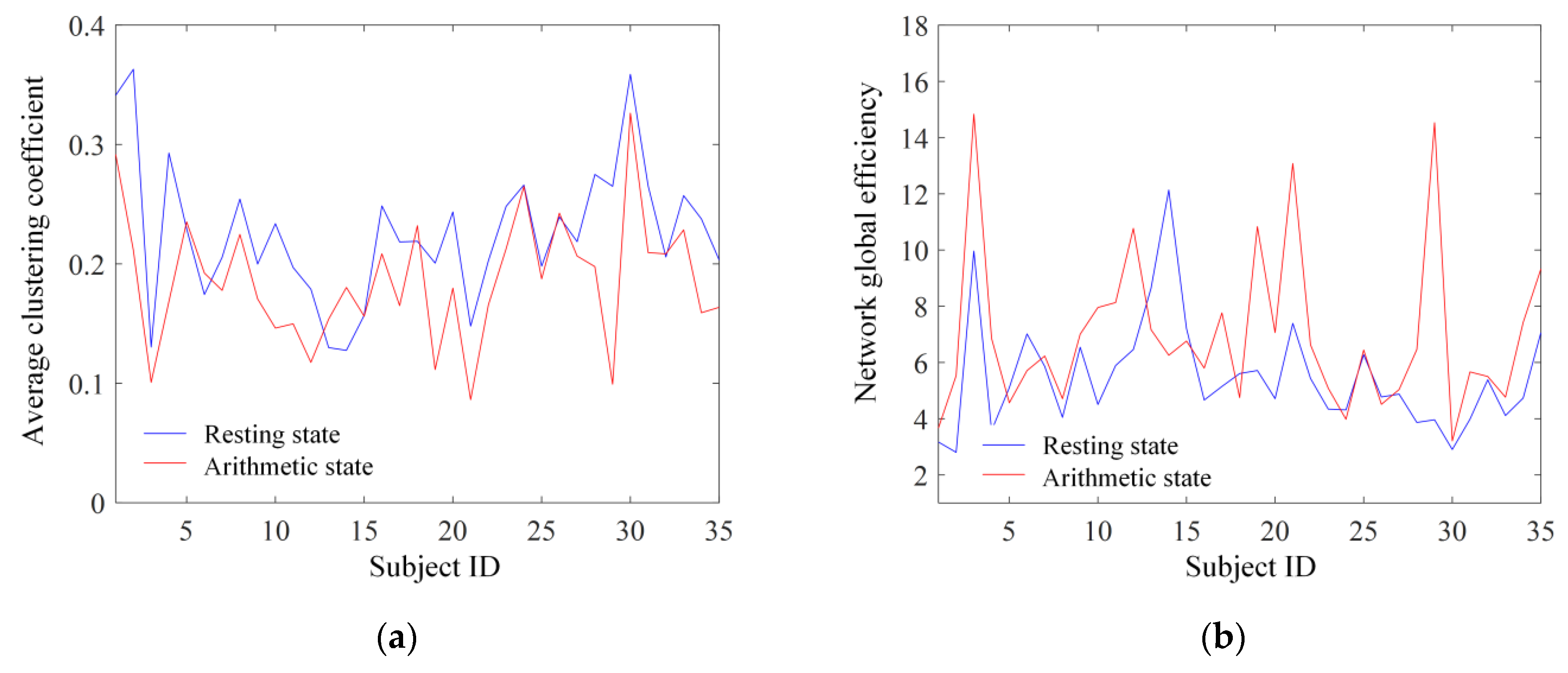
3.2. Analysis of Realistic EEG in Mental Arithmetic Tasks

In order to demonstrate the performance of the proposed CBTN method on realistic experimental data, the EEG signals of mental arithmetic tasks-dataset were used to distinguish the difference between the resting and the arithmetic states of the brain [41]. The dataset can be downloaded freely from the website: https://physionet.org/content/eegmat/1.0.0/, accessed on 23 January 2022. Electrodes were placed according to the international 10/20 scheme and the equipment used was the Neurocom monopolar EEG 23-channel system (Ukraine, XAI-MEDICA). The placement of the silver/silver chloride electrodes on the scalp was prefrontal (Fp1 and Fp2), frontal (F3, F4, Fz, F7, and F8), central (C3, C4, and Cz), parietal (P3, P4, and Pz), occipital (O1 and O2), and temporal (T3, T4, T5, and T6), all referenced to an interconnected ear reference electrode. The impedance between the electrodes and the scalp was less than 5 kΩ, and the sampling rate for each channel was 500 Hz. The acquired EEG signals were filtered using a high-pass filter with a cut-off frequency of 0.5 Hz, a low-pass filter with a cut-off frequency of 45 Hz, and a power line notch filter (50 Hz). The EEG data from 36 subjects (9 males and 27 females, aged 16–26 years) met the requirements for analysis, after a visual inspection of the filtered signals by neuroelectrophysiologists to remove data with poor signal quality. Subject 31 was not included because the length of the recordings was different from that of other subjects. The experiments involved mental arithmetic tasks and each experiment trial was divided into three phases: an adaptation period, a resting state and an arithmetic state. First, the subjects were acclimatized to the experimental conditions for 3 min. Afterwards, the subjects relaxed for 3 min with their eyes closed in the resting state. Finally, the subjects were asked to perform a succession of subtractions in 4 min, each consisting of a four-digit (subtracted number) and two-digit (subtracted number) succession. The two digits were given to the subject verbally and the arithmetic task was not allowed to be performed verbally, but finger movements were allowed. In order to minimize the effect of emotional fluctuations caused by the increased cognitive load of the subjects during intensive cognitive activity on the results of the EEG analysis, the last minute of the resting state and the first minute of the arithmetic state were selected for analysis. Neuroimaging studies showed that the prefrontal and frontal regions were significantly activated during the performance of arithmetic or cognitive tasks [42,43]. Therefore, EEG data collected from seven channels (FP1, FP2, F3, Fz, F4, F7, and F8) in the prefrontal and frontal lobes were used in this study, and the NOTE between any two channels was calculated using the CBTN method to construct an undirected weighted network with the NOTE as the edge weight. Network parameters were extracted from the constructed complex network as a quantitative evaluation indicator of cognitive load. Since the NOTE value is inversely correlated with the coupling strength, in the subsequent analysis, the NOTE values were reversely processed (1 minus the value of NOTE), so that they would adhere to our intuition.
EEG signals were first detrended using the singular value decomposition (SVD) method. Then, the detrended EEG signal was filtered using the harmonic wavelets in the frequency range of 1 to 42 Hz. The obtained resting and arithmetic state EEG signals from seven channels were segmented using a sliding time window with a width of 2000 samples and a moving step of 500 samples. Within each window, the NOTE was estimated between any two of the seven EEG channels using the CBTN method. With the NOTE value as the edge weight, the complex network was constructed and the average clustering coefficient and the global network efficiency of the complex network were calculated. Following the same procedure, all sliding windows were analyzed in turn to obtain the average aggregation coefficient sequence and the global network efficiency sequence of the subject in a state. Since the distribution of the obtained sequences were unknown, the nonparametric permutation test (1000 repeated arrangement sampling) was used to assess the significance between the same sequences in the two states of the subject. The significance level p was set to 0.05. As a comparison, the same operation was performed on this subject using the CPE method with an embedding dimension of 5 and a delay time of 8. The results of the significance analysis between the feature sequences for all the 35 subjects under the two method treatments are shown in Table 1. The values bolded in black in Table 1 indicate statistical insignificance between the two states. As can be seen from the results of the analysis in Table 1, the CBTN method is obviously superior to the CPE method.
In order to confirm whether there were group differences in the EEG signals between the resting and arithmetic states, the mean adjacency matrix of each subject was constructed using the CBTN, and the network parameters of the mean adjacency matrix were extracted for each subject. The same procedure was performed using the CPE as comparison. The EEG data within each sliding window were analyzed using the CBTN to build a complex network, and its adjacency matrix was obtained. All adjacency matrices from the same subject under the same state were averaged. The clustering coefficient and the global network efficiency of the average adjacency matrix were used as a feature for each subject. In this way, the feature in the two states was obtained for individual subjects. The results obtained for all subjects are shown in Figure 5. It can be seen that for most subjects, the mean clustering coefficient of the arithmetic state was smaller than that of the resting state and the global efficiency of the arithmetic state was greater than that of the resting state. This means that the network in the prefrontal area was more efficient and had enhanced information processing capacity during the arithmetic state. It also means an increased cognitive load during the arithmetic state. Figure 6 shows the analysis results of extracting the features of the complex network constructed by the CPE method under two states.
In order to verify whether there was significant difference between the two states at the group level, the results was statistically analyzed using a paired sample t-test. The significance level was set at p = 0.05, and statistical analysis was performed on IBM SPSS25.0. The results of the statistical analysis showed that there was a significant difference in the mean clustering coefficients (p = 0.0013) and in the global network efficiency (p = 0.0017) between the two states using the CBTN method (Figure 5). The results of the statistical analysis also showed that there was a significant difference in the mean clustering coefficients (p = 0.0056) and in the global network efficiency (p = 0.0061) between the two states using the CPE method. Although both methods can distinguish between the two states, the CBTN analysis was significantly better than the CPE analysis. This suggests that a complex network based on the CBTN using electrodes in the prefrontal and frontal lobe can distinguish well between the two cognitive states, demonstrating the validity of the CBTN method in practical applications.

4. Discussion

The aim of this study is to construct a complex network using multichannel EEG signals to enable the assessment of cognitive load. The method of constructing the network directly affects the reliability of the assessment. In the process of using CPE suitable for the analysis of short time series to construct complex networks, it was found that the CPE method suffered from the lack of differentiation ability caused by considering only the probability distribution of symbols and ignoring the transition relationship between symbols in the temporal domain. In addition, as a nonlinear analysis method, the choice of parameters in the CPE had a large impact on the analysis results. In order to alleviate these issues, the CBTN is proposed to measure the coupling relationship between two time series from the perspective of cross-transition networks. The innovation of the CBTN is that it combines the advantages of the transition network and the bubble entropy on the basis of the principle of CPE. The introduction of the transition network solved the problem of ignoring the transition relationship between symbols in the CPE method. The symbolization method with reference to bubble entropy made the analysis result less affected by the embedding dimension. The effectiveness of the method was verified via a comparison with the CPE method on the unidirectional coupled Henon model. Firstly, the results show that the CBTN method could achieve satisfactory results when the signal length reached 2000 samples, although this was slightly larger than that needed in the CPE method. This finding suggests that the CBTN is equally suitable for the analysis of short time series. Secondly, in the experiment study, the result tended to be stable for any coupling strength as long as the embedding dimension of the CBTN was greater than 10. This result indicates that the CBTN method is less affected by the coupling strength. Last, under weak coupling conditions, the CPE method failed to achieve the right results, while the CBTN could still obtain reliable results, indicating that the CBTN was able to uncover the weak coupling relationships between time series. These three properties ensure that the complex network constructed by the CBTN method outperformed the CPE in its ability to analyze cognitive load using EEG datasets. The results of the above analysis clearly demonstrate that the proposed method shows several advantages.
1. This method involves few parameters in use, and the value setting of the parameters has little influence on the analysis results.
2. The cross-transition network allows the method to be more sensitive to weak changes in the information interaction between two time series and is more suitable for analysis in weakly coupled conditions.
3. The normalization measures in the definition of node-wise out-link entropy minimize the impact of intersubject variation on the analysis results.
4. The implementation of the algorithm only involves the ranking of numbers and the probability distribution statistics of symbols, which is easy to be processed and implemented by a computer.
Although the study showed promising results, the limitation of this work should be considered. Firstly, the adjacency matrix of the cross-transition network was a static representation of information interaction between two time series in a period of time. This means that the method was explicitly time-dependent. The analysis of excessively long time series may have caused a reduction in the variation in the adjacency matrix, making identification less effective. This needs further study. Secondly, when using EEG datasets for cognitive load assessment, the electrodes used for analysis were determined subjectively only based on the findings of the neuroimaging, ignoring other aspects of the selection factors. As pointed out in the literature [44], in practical application, the practicality of electrode installation and the comfort of subjects should also be considered. Thirdly, the phase space reconstruction of the time series only considered the influence of the embedded dimension as a variable on the analysis results, and the time delay was set to 1 according to the bubble entropy. In the next research work, the comprehensive impact on the analysis results when these two parameters are variables will be studied in depth.

5. Conclusions

In this study, the advantages of the transition network and the bubble entropy were integrated based on the CPE method, and a new method to measure the coupling strength of two time series was proposed from the perspective of a cross-transition network. It was further used to build complex networks using the multichannel EEG recordings for cognitive load assessment. The results of the unidirectional coupled Honen model showed that this proposed method was not only suitable for the analysis of coupling strength between two short time series, but also had the advantages of being less affected by nonlinear parameters and sensitive to a weak coupling relationship. In addition, the proposed CBTN showed better performance in differentiating cognitive load than the CPE. The new method can be used for state evaluation based on multichannel physiological signals, such as brain state monitoring, quantitative evaluation of various types of mental diseases, and motion decoding based on multichannel electromyography (EMG). It also has an application potential in the financial research field.

Author Contributions

Conceptualization, X.C. and G.X.; methodology, X.C.; software, X.C. and X.Z.; validation, S.Z. and Z.T.; formal analysis, X.C.; investigation, X.C.; resources, S.Z.; data curation, X.C.; writing—original draft preparation, X.C.; writing—review and editing, X.C. and G.X.; visualization, X.Z.; supervision, G.X.; project administration, S.Z.; funding acquisition, S.Z. All authors have read and agreed to the published version of the manuscript.

Funding

This research was funded by the Scientific and Technological Innovation 2030, grant number: 2021ZD0204300 and the Xi’an City Innovation Capability Strengthening Basic Disciplines plan, grant number: 21RGSF0018 and the Key Projects in Shaanxi Province, grant number: 2021GXLH-Z-008).

Institutional Review Board Statement

Not applicable.

Informed Consent Statement

Not applicable.

Data Availability Statement

The raw data supporting the conclusions of this article will be made available by the authors, without undue reservation, to any qualified researcher.

Acknowledgments

We would like to thank all collaborators for their selfless help and guidance in research.

Conflicts of Interest

The authors declare no conflict of interest.

References

  1. Sweller, J. Cognitive load during problem solving: Effects on learning. Cogn. Sci. 1988, 12, 257–285. [Google Scholar] [CrossRef]
  2. Schnotz, W.; Kürschner, C. A reconsideration of cognitive load theory. Educ. Psychol. Rev. 2007, 19, 469–508. [Google Scholar] [CrossRef]
  3. Paas, F.; Tuovinen, J.E.; Tabbers, H.; Van Gerven, P.W. Cognitive load measurement as a means to advance cognitive load theory. In Educational Psychologist; Routledge, Taylor & Francis: London, UK, 2003; pp. 63–71. [Google Scholar]
  4. Useche, S.A.; Cendales, B.; Gómez, V. Measuring fatigue and its associations with job stress, health and traffic accidents in professional drivers: The case of BRT operators. EC Neurol. 2017, 4, 103–118. [Google Scholar]
  5. Soares, S.M.; Gelmini, S.; Brandao, S.S.; Silva, J. Workplace accidents in Brazil: Analysis of physical and psychosocial stress and health-related factors. RAM Rev. Adm. Mackenzie 2018, 19. [Google Scholar] [CrossRef]
  6. Burgess, D.J.; Phelan, S.; Workman, M.; Hagel, E.; Nelson, D.B.; Fu, S.S.; Widome, R.; van Ryn, M. The effect of cognitive load and patient race on physicians’ decisions to prescribe opioids for chronic low back pain: A randomized trial. Pain Med. 2014, 15, 965–974. [Google Scholar] [CrossRef] [PubMed] [Green Version]
  7. Hulbert, L.E.; Moisá, S.J. Stress, immunity, and the management of calves. J. Dairy Sci. 2016, 99, 3199–3216. [Google Scholar] [CrossRef] [Green Version]
  8. Yang, B.; Wang, Y.; Cui, F.; Huang, T.; Sheng, P.; Shi, T.; Huang, C.; Lan, Y.; Huang, Y.-N. Association between insomnia and job stress: A meta-analysis. Sleep Breath. 2018, 22, 1221–1231. [Google Scholar] [CrossRef]
  9. Heard, J.; Harriott, C.E.; Adams, J.A. A survey of workload assessment algorithms. IEEE Trans. Hum.-Mach. Syst. 2018, 48, 434–451. [Google Scholar] [CrossRef]
  10. Hart, S.G.; Staveland, L.E. Development of NASA-TLX (Task Load Index): Results of empirical and theoretical research. In Advances in Psychology; Elsevier: Amsterdam, The Netherlands, 1988; Volume 52, pp. 139–183. [Google Scholar]
  11. Reid, G.B.; Nygren, T.E. The subjective workload assessment technique: A scaling procedure for measuring mental workload. In Advances in Psychology; Elsevier: Amsterdam, The Netherlands, 1988; Volume 52, pp. 185–218. [Google Scholar]
  12. Hart, S.G. NASA-task load index (NASA-TLX); 20 years later. In Proceedings of the Human Factors and Ergonomics Society Annual Meeting, Los Angeles, CA, USA, 16–20 October 2006; pp. 904–908. [Google Scholar]
  13. Arico, P.; Borghini, G.; Di Flumeri, G.; Sciaraffa, N.; Colosimo, A.; Babiloni, F. Passive BCI in operational environments: Insights, recent advances, and future trends. IEEE Trans. Biomed. Eng. 2017, 64, 1431–1436. [Google Scholar] [CrossRef]
  14. Sibi, S.; Ayaz, H.; Kuhns, D.P.; Sirkin, D.M.; Ju, W. Monitoring driver cognitive load using functional near infrared spectroscopy in partially autonomous cars. In Proceedings of the 2016 IEEE Intelligent Vehicles Symposium (IV), Gothenburg, Sweden, 19–22 June 2016; pp. 419–425. [Google Scholar]
  15. Kadosh, R.C.; Kadosh, K.C.; Linden, D.E.; Gevers, W.; Berger, A.; Henik, A. The brain locus of interaction between number and size: A combined functional magnetic resonance imaging and event-related potential study. J. Cogn. Neurosci. 2007, 19, 957–970. [Google Scholar] [CrossRef]
  16. Murugesan, S.; Bouchard, K.; Chang, E.; Dougherty, M.; Hamann, B.; Weber, G.H. Hierarchical spatio-temporal visual analysis of cluster evolution in electrocorticography data. In Proceedings of the 7th ACM International Conference on Bioinformatics, Computational Biology, and Health Informatics, Seattle, WA, USA, 2–5 October 2016; pp. 630–639. [Google Scholar]
  17. Antonenko, P.; Paas, F.; Grabner, R.; Van Gog, T. Using electroencephalography to measure cognitive load. Educ. Psychol. Rev. 2010, 22, 425–438. [Google Scholar] [CrossRef]
  18. Örün, Ö.; Akbulut, Y. Effect of multitasking, physical environment and electroencephalography use on cognitive load and retention. Comput. Hum. Behav. 2019, 92, 216–229. [Google Scholar] [CrossRef]
  19. Tor, H.T.; Ooi, C.P.; Lim-Ashworth, N.S.; Wei, J.K.E.; Jahmunah, V.; Oh, S.L.; Acharya, U.R.; Fung, D.S.S. Automated detection of conduct disorder and attention deficit hyperactivity disorder using decomposition and nonlinear techniques with EEG signals. Comput. Methods Programs Biomed. 2021, 200, 105941. [Google Scholar] [CrossRef] [PubMed]
  20. Wiersma, M. Identifying workload levels with a low-cost EEG device using an arithmetic task. In Faculty of Science and Engineering; Macquarie University: Sydney, Australia, 2016. [Google Scholar]
  21. Acharya, U.R.; Chua, C.K.; Lim, T.-C.; Dorithy; Suri, J.S. Automatic identification of epileptic EEG signals using nonlinear parameters. J. Mech. Med. Biol. 2009, 9, 539–553. [Google Scholar] [CrossRef]
  22. Salankar, N.; Qaisar, S.M.; Paweł Pławiak, P.é.; Tadeusiewicz, R.; Hammad, M. EEG based alcoholism detection by oscillatory modes decomposition second order difference plots and machine learning. Biocybern. Biomed. Eng. 2022, 42, 173–186. [Google Scholar] [CrossRef]
  23. Shahbakhti, M.; Beiramvand, M.; Eigirdas, T.; Solé-Casals, J.; Wierzchon, M.; Broniec-Wójcik, A.; Augustyniak, P.; Marozas, V. Discrimination of Wakefulness from Sleep Stage I Using Nonlinear Features of a Single Frontal EEG Channel. IEEE Sens. J. 2022, 22, 6975–6984. [Google Scholar] [CrossRef]
  24. Paul, J.K.; Iype, T.; Dileep, R.; Hagiwara, Y.; Koh, J.W.; Acharya, U.R. Characterization of fibromyalgia using sleep EEG signals with nonlinear dynamical features. Comput. Biol. Med. 2019, 111, 103331. [Google Scholar] [CrossRef]
  25. Varela, F.; Lachaux, J.-P.; Rodriguez, E.; Martinerie, J. The brainweb: Phase synchronization and large-scale integration. Nat. Rev. Neurosci. 2001, 2, 229–239. [Google Scholar] [CrossRef]
  26. Bullmore, E.; Sporns, O. Complex brain networks: Graph theoretical analysis of structural and functional systems. Nat. Rev. Neurosci. 2009, 10, 186–198. [Google Scholar] [CrossRef]
  27. Shang, J.; Zhang, W.; Xiong, J.; Liu, Q. Cognitive load recognition using multi-channel complex network method. In Proceedings of the International Symposium on Neural Networks, Sapporo, Hakodate, Muroran, Japan, 21–26 June 2017; pp. 466–474. [Google Scholar]
  28. Kakkos, I.; Dimitrakopoulos, G.N.; Gao, L.; Zhang, Y.; Qi, P.; Matsopoulos, G.K.; Thakor, N.; Bezerianos, A.; Sun, Y. Mental workload drives different reorganizations of functional cortical connectivity between 2D and 3D simulated flight experiments. IEEE Trans. Neural Syst. Rehabil. Eng. 2019, 27, 1704–1713. [Google Scholar] [CrossRef]
  29. Shovon, M.; Islam, H.; Nandagopal, N.; Vijayalakshmi, R.; Du, J.T.; Cocks, B. Directed connectivity analysis of functional brain networks during cognitive activity using transfer entropy. Neural Process. Lett. 2017, 45, 807–824. [Google Scholar] [CrossRef]
  30. Suresh, K.; Ramasamy, V.; Daniel, R.; Chandra, S. Characterizing EEG Electrodes in Directed Functional Brain Networks Using Normalized Transfer Entropy and PageRank. In Handbook of Artificial Intelligence in Healthcare; Springer: Berlin/Heidelberg, Germany, 2022; pp. 27–49. [Google Scholar]
  31. Wang, J.; Wang, L.; Zang, Y.; Yang, H.; Tang, H.; Gong, Q.; Chen, Z.; Zhu, C.; He, Y. Parcellation-dependent small-world brain functional networks: A resting-state fMRI study. Hum. Brain Mapp. 2009, 30, 1511–1523. [Google Scholar] [CrossRef] [PubMed]
  32. Steuer, R.; Kurths, K., Jr.; Daub, C.O.; Weise, J.; Selbig, J. The mutual information: Detecting and evaluating dependencies between variables. Bioinformatics 2002, 18, S231–S240. [Google Scholar] [CrossRef] [PubMed] [Green Version]
  33. Vejmelka, M.; Paluš, M. Inferring the directionality of coupling with conditional mutual information. Phys. Rev. E 2008, 77, 026214. [Google Scholar] [CrossRef] [Green Version]
  34. Schreiber, T. Measuring information transfer. Phys. Rev. Lett. 2000, 85, 461. [Google Scholar] [CrossRef] [Green Version]
  35. Hempel, S.; Koseska, A.; Kurths, K., Jr.; Nikoloski, Z. Inner composition alignment for inferring directed networks from short time series. Phys. Rev. Lett. 2011, 107, 054101. [Google Scholar] [CrossRef] [Green Version]
  36. Liu, L.-Z.; Qian, X.-Y.; Lu, H.-Y. Cross-sample entropy of foreign exchange time series. Phys. A Stat. Mech. Its Appl. 2010, 389, 4785–4792. [Google Scholar] [CrossRef]
  37. Shu, Y.; Zhao, J. Data-driven causal inference based on a modified transfer entropy. Comput. Chem. Eng. 2013, 57, 173–180. [Google Scholar] [CrossRef]
  38. Kiwata, H. Relationship between Schreiber’s transfer entropy and Liang-Kleeman information flow from the perspective of stochastic thermodynamics. Phys. Rev. E 2022, 105, 044130. [Google Scholar] [CrossRef]
  39. Shi, W.; Shang, P.; Lin, A. The coupling analysis of stock market indices based on cross-permutation entropy. Nonlinear Dyn. 2015, 79, 2439–2447. [Google Scholar] [CrossRef]
  40. Manis, G.; Aktaruzzaman, M.D.; Sassi, R. Bubble Entropy: An Entropy almost Free of Parameters. IEEE Trans. Bio-Med. Eng. 2017, 64, 2711–2718. [Google Scholar]
  41. Zyma, I.; Tukaev, S.; Seleznov, I.; Kiyono, K.; Popov, A.; Chernykh, M.; Shpenkov, O. Electroencephalograms during mental arithmetic task performance. Data 2019, 4, 14. [Google Scholar] [CrossRef]
  42. Yu, J.; Pan, Y.; Ang, K.K.; Guan, C.; Leamy, D.J. Prefrontal cortical activation during arithmetic processing differentiated by cultures: A preliminary fNIRS study. In Proceedings of the 2012 Annual International Conference of the IEEE Engineering in Medicine and Biology Society, San Diego, CA, USA, 28 August–1 September 2012; pp. 4716–4719. [Google Scholar]
  43. Menon, V.; Mackenzie, K.; Rivera, S.M.; Reiss, A.L. Prefrontal cortex involvement in processing incorrect arithmetic equations: Evidence from event-related fMRI. Hum. Brain Mapp. 2002, 16, 119–130. [Google Scholar] [CrossRef] [PubMed]
  44. Shahbakhti, M.; Beiramvand, M.; Rejer, I.; Augustyniak, P.; Broniec-Wojcik, A.; Wierzchon, M.; Marozas, V. Simultaneous eye blink characterization and elimination from low-channel prefrontal EEG signals enhances driver drowsiness detection. IEEE J. Biomed. Health Inform. 2021, 26, 1001–1012. [Google Scholar] [CrossRef]
Figure 1. The directional weighted adjacency matrix constructed from the temporal adjacency relationship for symbol sets A and B. (a) The adjacency matrix for the symbolized set A; (b) The adjacency matrix for the symbolized set B.
Applsci 12 11165 g001
Figure 2. The results of the unidirectional coupled Henon model using CBTN and CPE for coupling analysis, respectively, at different coupling strengths C = 0.1 , 0.3 , 0.5 and when the sliding time window width is varied in steps of 200 samples within [200, 5000]. The values of the ordinate are H x 1 x 2 s u r r o g a t e H x 1 x 2 . x 2 s u r r o g a t e can be obtained by surrogating x 2 using the iAAFT method. (a) The results of coupling analysis using CBTN (30 repeated calculations); (b) The results of coupling analysis using CPE, d = 5 , τ = 2 (30 repeated calculations).
Applsci 12 11165 g002
Figure 3. At different coupling strengths C = 0.1 , 0.3 , 0.5 , the sliding time window width is fixed at 2000 samples, and the embedding dimension d is taken from 3 to 15; the results of unidirectional coupled Henon model using CBTN and CPE for coupling analysis, respectively. The values of ordinate are H x 1 x 2 s u r r o g a t e H x 1 x 2 . x 2 s u r r o g a t e can be obtained by surrogating x 2 using the iAAFT method. (a) The results of coupling analysis using CBTN (30 repeated calculations); (b) The results of coupling analysis using CPE, τ = 2 (30 repeated calculations).
Applsci 12 11165 g003
Figure 4. Coupling analysis results for the CBTN-based unidirectional coupled Henon model when the sliding time window is fixed at 2000 samples and the coupling strength C is varied in steps of 0.05 in the range [0, 0.9]. The values of the ordinate are H N O T E . The blue curve is the NOTE between x 1 and x 2 and the red curve is the NOTE between x 1 and x 2 s u r r o g a t e . x 2 s u r r o g a t e can be obtained by surrogating x 2 using the iAAFT method (all values in the graph are the result of 30 repeated calculations). (a) The results of coupling analysis using CBTN. (b) The results of coupling analysis using CPE, d = 5 , τ = 2 .
Applsci 12 11165 g004
Figure 5. The average clustering coefficient (a) and global network efficiency (b) of the average adjacency matrix constructed by the CBTN method for each subject.
Applsci 12 11165 g005
Figure 6. The average clustering coefficient (a) and global network efficiency (b) of the average adjacency matrix constructed by the CPE method for each subject.
Applsci 12 11165 g006
Table 1. Results of nonparametric permutation tests for each subject’s feature sequences in the resting and arithmetic states (1000 repeated arrangement sampling, significant level p = 0.05).
CBTNCPE
ACEGNEACEGNE
Subject 00000
Subject 10000
Subject 20.0040.00100
Subject 30000
Subject 40.9730.5400.6650
Subject 5000.5180.342
Subject 60000
Subject 70000
Subject 80000
Subject 90000
Subject 100000
Subject 110000
Subject 120.0050.01800
Subject 130000
Subject 140.6460.83200.018
Subject 150000
Subject 160000
Subject 170.1250.1580.3980.035
Subject 180000
Subject 190000
Subject 200000
Subject 210000
Subject 22000.0010.021
Subject 23000.1860.680
Subject 24000.0050.004
Subject 250.0110.0070.4830.603
Subject 26000.0490.08
Subject 270000
Subject 280000
Subject 290000
Subject 300000
Subject 32000.5910.895
Subject 330000
Subject 340000
Subject 350000
ACE (average clustering coefficients), GNE (global network efficiency). Non significant results are shown in bold.
Publisher’s Note: MDPI stays neutral with regard to jurisdictional claims in published maps and institutional affiliations.

