
OTSU Multi-Threshold Image Segmentation Based on Improved Particle Swarm Algorithm


1
School of Mechanical Engineering and Rail Transit, Changzhou University, Changzhou 213164, China
2
Jiangsu Province Engineering Research Center of High-Level Energy and Power Equipment, Changzhou University, Changzhou 213164, China
3
Key Laboratory of Noise and Vibration, Institute of Acoustics, Chinese Academy of Sciences, Beijing 100190, China
*
Author to whom correspondence should be addressed.
Appl. Sci. 2022, 12(22), 11514; https://0-doi-org.brum.beds.ac.uk/10.3390/app122211514
Submission received: 21 September 2022
/
Revised: 7 November 2022
/
Accepted: 9 November 2022
/
Published: 13 November 2022
(This article belongs to the Special Issue Scale Space and Variational Methods in Computer Vision)
Abstract
:In view of the slow convergence speed of traditional particle swarm optimization algorithms, which makes it easy to fall into local optimum, this paper proposes an OTSU multi-threshold image segmentation based on an improved particle swarm optimization algorithm. After the particle swarm completes the iterative update speed and position, the method of calculating particle contribution degree is used to obtain the approximate position and direction, which reduces the scope of particle search. At the same time, the asynchronous monotone increasing social learning factor and the asynchronous monotone decreasing individual learning factor are used to balance global and local search. Finally, chaos optimization is introduced to increase the diversity of the population to achieve OTSU multi-threshold image segmentation based on improved particle swarm optimization (IPSO). Twelve benchmark functions are selected to test the performance of the algorithm and are compared with the traditional meta-heuristic algorithm. The results show the robustness and superiority of the algorithm. The standard dataset images are used for multi-threshold image segmentation experiments, and some traditional meta-heuristic algorithms are selected to compare the calculation efficiency, peak signal to noise ratio (PSNR), structural similarity (SSIM), feature similarity (FSIM), and fitness value (FITNESS). The results show that the running time of this paper is 30% faster than other algorithms in general, and the accuracy is also better than other algorithms. Experiments show that the proposed algorithm can achieve higher segmentation accuracy and efficiency.
1. Introduction
Image segmentation is widely used as the basis of computer vision. Image segmentation refers to describing an image as a collection of some connected areas so that the image features are different in different areas. At present, image segmentation methods mainly include the threshold method, edge detection method, region method, morphological watershed method, and so on [1]. The threshold method is at the core of image segmentation applications because of its simple implementation and fast calculation speed [2]. Thresholds can be divided into two forms, namely, two-stage thresholds (BT) and multilevel thresholds (MT). The two-level threshold uses a single threshold to divide the image into two categories, and the multi-level threshold uses multiple thresholds to divide the image into more than two uniform segments [3]. The threshold can be determined by kapur entropy [4], Tsallis entropy [5], fuzzy entropy [6], and OTSU variance [7]. This method uses the information in the histogram and does not need any ground live to classify pixels. However, threshold policy is a time-consuming process, especially when increasing the number of thresholds. The running time will greatly increase, so this has become a problem that must be solved in future research.
Recently, Houssein et al. proposed an improved balance optimizer to solve the problem of imbalance between the exploration stage and the development stage of the balance optimizer, which solves the problem that the algorithm optimization is easy to fall into local optimization and shows the excellent performance of this algorithm [8]. Sharma, Sushmita, and others improved the original butterfly optimization algorithm by combining the mutualism and parasitic stages of the traditional butterfly algorithm and the symbiotic biological search algorithm. Using kapur entropy as the fitness function, they selected a group of benchmark images to find the optimal threshold. The results show that the improved butterfly algorithm is superior to other algorithms in all evaluation indicators [9]. In addition, Elaziz et al., in view of the shortcomings of the Harris Hawks Optimizer algorithm, proposed an improved version of the HHO algorithm, which solved the problem of poor search ability of traditional algorithms and makes it easy to fall into local optimization [10]. Zhang et al. proposed an improved PSO algorithm to solve the problem of premature convergence of traditional PSO and effectively realize adaptive image segmentation [11]. Zhao et al. proposed a cross strategy-based ant colony algorithm (CCACO) in order to solve the continuity problem of the ant colony algorithm, which uses Kapur entropy as the objective function for image segmentation. Experiments show that the proposed CCACO achieved excellent segmentation results in both low-threshold and high-threshold [12].
Of course, in the process of image segmentation, it is far from enough to rely only on threshold segmentation. Because of the low processing speed and segmentation accuracy of threshold segmentation, people will use optimization algorithms to optimize the segmentation process. Among many optimization algorithms, the meta-heuristic optimization algorithm is widely used because of its low cost, high accuracy, and fast speed. So far, various optimization algorithms have been introduced to deal with nonlinear and practical applications, such as genetic algorithm (GA) [13], particle swarm optimization (PSO) [14], whale optimization algorithm (WOA) [15], butterfly optimization algorithm (BOA) [9], sine cosine optimization algorithm (SCA) [16], crow optimization algorithm (CSA) [17], gray wolf optimization algorithm (GWO) [18], and bee colony optimization algorithm (ABC) [19]. In recent years, Raj et al. proposed the Whale Optimization Algorithm (WOA) to optimize TCSC and SVC reactive power planning for the problems of transmission loss and high operating costs. The results show that this method has fewer iterations, will not fall into local minimum, and has good convergence characteristics [15]. Shiva and Gudadappanavar proposed an opposite crow search algorithm for transmission loss, which has better performance in reducing active power and system operation cost [16]. In order to solve the problems of insufficient reactive power and unstable voltage of transmission lines, Babu and Kumar et al. proposed an improved sine cosine optimization algorithm, which uses the techniques of the sine cosine algorithm (SCA) and quasi inverse sine cosine algorithm (QOSCA) to minimize transmission losses and operating costs [17]. Xu et al. proposed an improved hunger game search algorithm (IHGS) for solar photovoltaic system parameter identification, which solved the problem of stability of the algorithm when solving the global optimal solution. It shows the feasibility and effectiveness of the improved HGS algorithm [20]. In addition, Trojovsky et al. proposed a new population-based optimization algorithm, the Pelican Algorithm (POA). This algorithm has high development and strong search ability [21]. Shabani and Asgarian put forward the search and rescue optimization algorithm (SAR) for the problem of single objective continuous optimization and demonstrated the feasibility of the algorithm through experiments [22]. Oliva and Elizabeth put forward a new solution to the problem that the traditional algorithm population is small and easy to fall into the local optimum. They used chaos mapping and opposite learning to initialize the solution of the given problem and improve the diversity of the population by constantly following the new initial population position through the interference operator. The experimental results show that the proposed method has high efficiency in dealing with the optimal solution problem [23].
In order to improve the performance of PSO on image threshold segmentation, a new OTSU multi-threshold segmentation method based on Improved PSO was proposed. The selection process of thresholds were optimized and compared with many classical PSO methods. The results show that our algorithm reduces the running time and improves the accuracy in threshold segmentation. The main contributions in this paper can be summarized as follows:
- (1)
- An Improved PSO algorithm is proposed, in which (a) chaos optimization was added to reduce premature convergence; (b) elite particle search strategy to particle swarm optimization algorithm was used to reduce optimization time and improve efficiency; (c) learning factors were improved to balance local search and global search.
- (2)
- Combining PSO with OTSU algorithm, a gray image segmentation algorithm based on improved particle swarm optimization is proposed. The proposed improved particle swarm optimization segmentation algorithm can search for a more accurate threshold, thus promoting better component division of gray-scale images.
- (3)
- Some classical test functions are selected to verify the robustness and development of the algorithm in solving single peak, multi-peak, and multi-peak fixed dimension functions.
- (4)
- Compared with the multi threshold segmentation of some standard algorithms, the performance of the improved PSO segmentation algorithm was verified, and the effectiveness of the algorithm on images was verified through multi-threshold image segmentation experiments on PASCAL 2012 dataset images. Experiments show that the method in this paper is faster than other meta heuristic algorithms in OTSU threshold segmentation, and PSNR FSIM and SSIM performance indicators verify that the algorithm in this paper has higher accuracy in image segmentation.
The rest of this paper is organized as follows: Section 2 summarizes the multi-threshold OTSU segmentation model. Section 3 describes the PSO algorithm. Section 4 proposes a multi-threshold segmentation algorithm based on the Improved PSO algorithm. Section 5 describes the experimental results of the segmentation method based on the improved particle swarm optimization. Section 6 presents conclusions and future work.
2. Multi-Threshold OTSU Segmentation Model
The OTSU image segmentation method is the maximum inter-class variance method, which aims to determine the optimal threshold for image segmentation. In OTSU, the image is divided into foreground and background by threshold, and the threshold with the largest class variance in the foreground and background regions is taken as the best segmentation threshold. Assume that the gray scale range is , representing L different gray levels in a digital image, whose size is pixels. Let be the proportion of grayscale i in the entire image, calculated as
where is the number of pixels with grayscale i. Let the threshold t divide the image into two parts, foreground and background.
where is the average grayscale of the image, which can be expressed as:
where and are the proportion of the foreground and background in the image, respectively, and and are the average grayscale of the image foreground and background, respectively. is the inter class variance, which can be expressed as:
when the interclass variance reaches the maximum, t is the optimal threshold. In the case of multiple thresholds, a threshold set of is the optimal combination of thresholds. The optimization problem can be expressed as:
The OTSU multi-threshold method uses the exhaustive method to solve the optimal thresholds combination with a total computational cost of O(). It can be seen that the computational cost will increase exponentially with the increase in the number of thresholds. In order to improve the efficiency of image segmentation, this paper proposes an improved particle swarm optimization algorithm to optimize the optimal threshold combination and then perform multi-threshold image segmentation.
3. Particle Swarm Algorithm
Particle swarm optimization (PSO) is a popular intelligent optimization algorithm [24] whose origins originate from the research on the predatory behaviors of birds. The PSO algorithm is similar to the genetic algorithm in that the solution of the objective function needs to be initialized randomly and optimized by iteration, without the crossover and mutation of chromosomes. Each particle is abstracted as a bird in the search space, which represents the solution of the optimization problem. The particle has two attributes: speed and position. The former represents the speed of movement and the latter represents the direction of movement. Substituting particle position information and velocity information into the fitness function to be optimized, the fitness value can be obtained. In the process of optimization, the particle determines its next motion through its own flight experience (individual extreme value) and group experience (group extreme value).
In a D-dimensional search space, the particle population size m, particle position , and velocity are initialized, where D = 1, m = 50, range of position X is [0, 255], and the range of velocity V is . Particle i individual extremes and Global Extremums is the optimal position currently searched by the particle, and is the optimal position currently searched by all of the particles. Over the course of each iteration, particles update their velocity and position according to the following equation:
where , , k is the number of iterations, and and are random numbers between ; these two parameters are used to maintain the diversity of the population. Furthermore, and are learning factors. Take , inertia weight reflects the ability of particles to inherit the previous velocity, with a linear decrement method, as follows:
where , , k is the number of iterations, is the total number of iterations, and .
4. Multi-Threshold Segmentation Algorithm Based on Improved PSO
The classical PSO algorithm is an effective method to deal with the optimization problem of threshold segmentation. However, due to the mechanism of particle swarm optimization algorithm, when used in image processing, a large number of calculations will make the image processing time longer, and premature convergence will fall into local optimization, thus reducing the overall work efficiency and affecting the accuracy of threshold segmentation. This paper proposes an improved particle swarm optimization algorithm to optimize OTSU multi-threshold image segmentation. The speed and accuracy of multi-threshold image segmentation are improved by optimizing the basic parameters of the particle swarm optimization algorithm and proposing an elite particle search strategy based on the classical particle swarm optimization algorithm.
4.1. Linear Optimization Learning Factor
For the problem of low segmentation accuracy of the classical particle swarm algorithm, a linear function is introduced in the process of parameter optimization of the particle swarm algorithm to update the learning factor of particles, and the changes in learning factors and affect individual and swarm particles to approach the optimal solution, respectively. Most of the search results from global search to local search are particles, and the centers of gravity of particle searches are also different at different stages. To mitigate this issue, this paper uses asynchronous linear decrement and asynchronous linear incrementing learning factors to balance global search and local search, so that the learning factor can change with the procedure of iterations. According to the characteristics of the PSO algorithm, in the early iterations, it is more likely to rely on the mobile experiences of particle individuals for global search, while in the later iteration, it mainly relies on the mobile experience of the group for local search. The PSO algorithm can enhance the global search ability by taking the larger value of the learning factor the smaller value of in the early iterations, and the smaller value of the larger value of in the later stages can enhance the local search ability. In order to better play the global search ability and local search ability at different stages and improve the accuracy of the segmentation, we use the asynchronous change learning factor. The formula is:
where and are the maximum and minimum values of the learning factor, , ; k and are the current number of iterations and the maximum number of iterations, respectively. The improved speed update formula is:
4.2. Elite Particle Search Strategy
In view of the low efficiency and slow speed of classical particle swarm optimization in multi-threshold segmentation, this paper improves classical particle swarm optimization by updating the speed and position of particles and proposes a search strategy for elite particles, which is divided into three steps. Firstly, the threshold segmentation contribution of each particle is calculated; secondly, 20% elite particles are selected according to the threshold segmentation contribution of each particle; and finally, the optimal solution of this iteration is found through chaos optimization.
In this paper, 20% of the particles are selected as elite particles according to the contribution. The contribution of each particle is obtained by comparing the fitness value of each particle with the fitness value of the global extremum in the current iteration. We calculated the distance difference between the location of a single particle and the location of the global limit particle. The closer the distance was to the optimal threshold, the greater the contribution to the optimization. Assuming that the global extremum particle is in each iteration, the distance difference between the location of a single particle and the location of the global extreme particle and the threshold segmentation contribution value of each single particle are obtained according to the following formula:
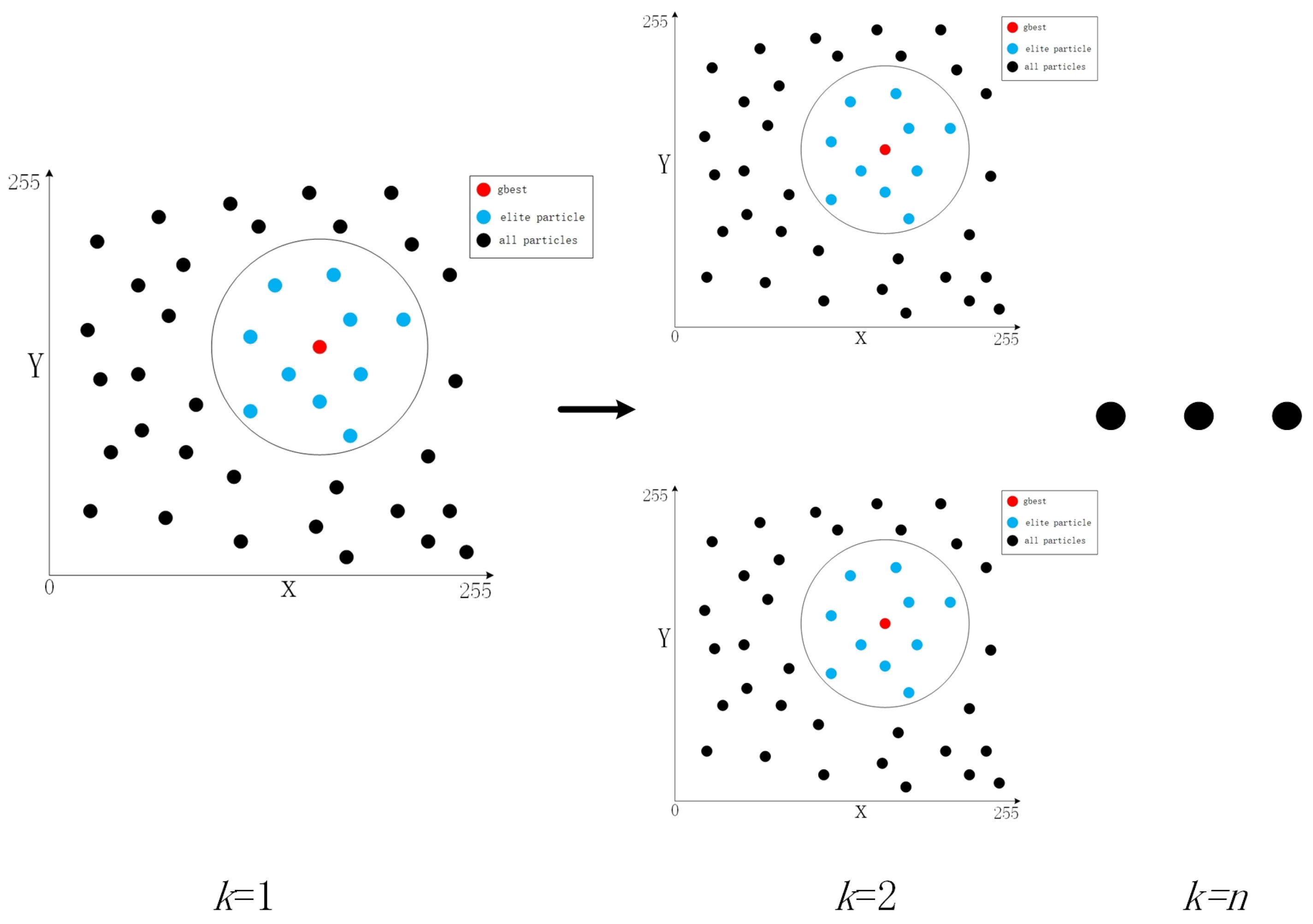
where z represents the distance between the individual particle of the ith particle and the particle individual, corresponding to the global extremum, is the x-axis of the particle individual, corresponding to the global extremum in the target search space, is the y-axis coordinate of the particle individual, corresponding to the global extremum in the target search space, is the x-axis of the i-th particle individual in the target search space, is the y-axis coordinate of the ith particle individual in the target search space, (actual contribution degree) is the threshold segmentation contribution of each particle, threshold segmentation contribution, and distance difference of z, which is inversely proportional. The closer the i-th particle individual is to the particle individual, corresponding to the global extreme value, the greater the contribution of the i-th particle individual to the threshold segmentation of this optimization. The top 20% of elite particles are selected in order of contribution from largest to smallest by threshold segmentation, reducing optimization time. For details, see Figure 1. Where the arrows represent the change in the number of thresholds, and the three circles indicate the optimization when the threshold is a different value.
Taking the gray value range of the segmented image as the coordinate range of x and y values, the black dot as all particles, and the central red dot as the global optimal solution of the current iteration, the search range can be reduced to a black circular region, that is, the region where the elite particles are located, and k is the number of threshold values. Each threshold requires a corresponding particle swarm to determine, while n threshold values require n particle swarms. In the same iteration, determine the global optimal particle of the n-particle swarm in turn.
Put the selected elite particles into chaos optimization. During each iteration, the is scrambled and used as the update position of the particles, which makes them search locally for the global optimal solution. The purpose is to increase the diversity of the population, enhance the local optimization ability of the algorithm, and realize the local depth search of the particle swarm algorithm. In order to solve the problem of premature convergence of particle swarm optimization algorithm and easy to fall into local optimization, so as to improve the accuracy of image segmentation chaos, the specific steps of chaos optimization elite particles are as follows:
Step 1. Set the number of chaotic iterations to M and map through Equation (15) to the defining domain of the Logistic equation [0, 1];
where, is the sequence element obtained by the first iteration, is the global extremum in the whole population, is the minimum value of the particle position, and is the maximum value of the particle position.
Step 2. is obtained after M iterations through Equation (16), and the chaotic sequence is obtained.
where is the sequence element obtained by the (n+1)-thi iteration, is the control parameter, and is the sequence element obtained by the M-th iteration.
Step 3. The chaotic sequence is inversely mapped back to the original solution space through Equation (17) to obtain the feasible solution sequence of chaotic variables
where is the sequence element obtained by the m-th iteration, .
Step 4. Calculate the fitness value of each feasible solution vector in the feasible solution sequence and retain the optimal vector, denoted as .
Step 5. Randomly select a particle from the current particle swarm and replace the position vector of the selected particle with a .
Step 6. Iterate until the maximum number of iterations is reached or gets a sufficiently satisfactory solution.
4.3. Our Method and Process
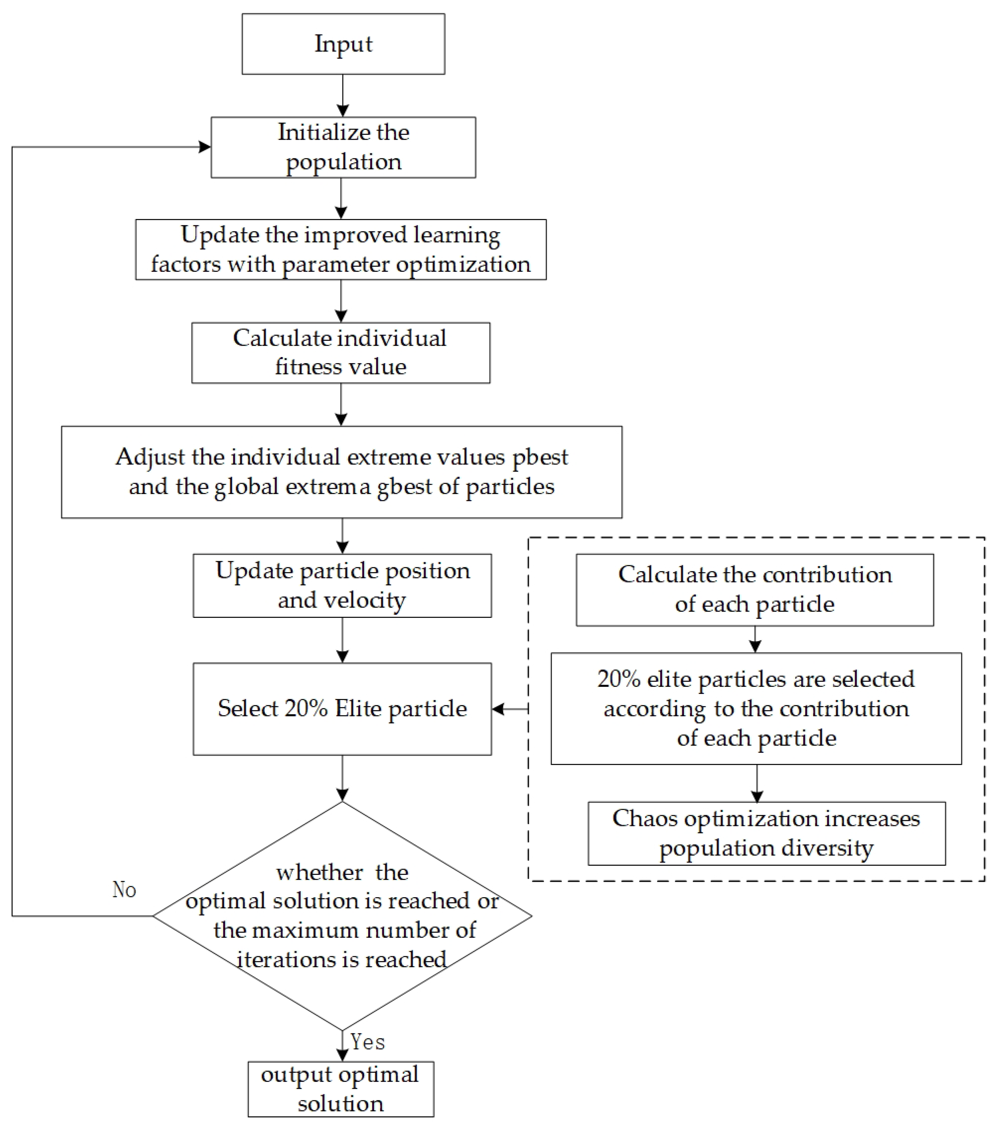
Compared with the classical particle swarm optimization algorithm, our improved particle swarm optimization algorithm is superior to the classical algorithm in terms of both speed and accuracy. At the same time, it also avoids the problem that the particle swarm optimization algorithm is prone to fall into local optimization, greatly improving the efficiency of image segmentation. The flow chart of our improved particle swarm optimization algorithm is shown in Figure 2.
To a certain extent, linear learning factors and elite particle search strategies are added to the classical particle swarm algorithm, which improves the problems of slow optimization speed, low precision, low efficiency, and easy optimization in the classical particle swarm. The detailed process based on the improved particle swarm algorithm is as follows:
Step 1. Set the parameters, which include the population size (m), dimension , velocity range , position range , and maximum number of iterations .
Step 2. Initialize the population. Initialize the dimensions and vectors of particle individuals according to the threshold number . The range of position vectors is [0255].
Step 3. Update and with asynchronous monotonically decreasing individual learning factor and asynchronous monotonically increasing social learning factor, and , instead of Equations (10) and (11) to individual, thereby improving the accuracy of particle optimization. Calculate the fitness values for individual particles, updating the individual extremums of particles and the global extremums of particles.
Step 4. Iteratively update the position of the particle individual and the speed of the particle individual.
Step 5. 20% elite particles are selected according to the threshold segmentation contribution of individual particles.
Step 6. Use chaotic iterative optimization to find the best fitness value for elite particles by comparing the chaotic optimization results.
Step 7. Determine whether the current number of chaotic iterations meets the set maximum number of chaos iterations or whether the chaos optimization reaches preset accuracy. If the current number of chaos iterations meets the maximum number of chaotic iterations or the chaos optimization reaches the set accuracy, go to step 8; otherwise, go to step 2.
Step 8. Map the optimal fitness value inversely back into the particle cluster group, calculate the fitness value of all particles in the particle cluster, and output the optimal solution if the set conditions are met; otherwise, go to step 1.
5. Experimental Analysis
5.1. Experimental Environment
Experiments demonstrate the effectiveness of our improved multi-threshold image segmentation algorithm. The test image is taken from the PASCAL 2012 data set [25]. The experimental environment consists of MATLAB 2018a, Windows 10, and an Intel(R) Core(TM) i5-5600H @ 2.4GHz CPU with 8GB of RAM. We set population size , maximum number of iterations , particle position range , velocity range , individual learning factor , and social learning factor .
5.2. Benchmark Function
This paper selects 12 standard test functions for comparative experiments to test the robustness, exploration, and development performance of the functions. These functions were derived from the CEC benchmark function [26], covering unimodal functions (F1–F4), multimodal functions (F5–F8), and fixed dimensional multimodal functions (F9–F12), all of which had minimum values. The algorithm compared with this paper uses the traditional meta-heuristic algorithms, which are whale optimization algorithm (WOA) [27], butterfly optimization algorithm [28], and particle swarm optimization algorithm [14]. In order to make a fair evaluation, this paper conducted 30 experiments on four optimization algorithms at the same time, and the experimental results less than are represented by 0.
Table 1 shows the selected test functions: Dim is the number of variables and N\A is unsolvable. Table 2 shows the average value and standard deviation of the benchmark function calculated by this method and the traditional meta heuristic algorithm. According to the data in Table 2, our method is robust in dealing with the mechanism of benchmark function, whether it is unimodal, multimodal, or a fixed-dimensional multimodal function. From Table 2, we can see that our method has better performance than WOA, BOA, and PSO. In particular, there is a smaller error in multimodal function, which shows that the method in this paper has better exploration capability. We found that our method did not find the global minimum in several functions, but the error was smaller than other algorithms. To sum up, our method was more exploitative and exploratory than other algorithms. The specific experiments are as follows:
5.3. Segmentation Experiment and Results
We took the optimization time and image segmentation quality to evaluate the performance of algorithms for comparison. The segmentation quality was evaluated with peak signal-to-noise ratio (PSNR) [29,30], structural similarity (SSIM) [31,32], and feature similarity (FSIM) [33,34], and fitness values of all algorithms were calculated. PSNR was used to evaluate the degree of image distortion, and the higher its value, the smaller the image distortion. SSIM evaluated image segmentation performance from image contrast and structural information. The larger the value, the better the performance. FSIM was used to evaluate the feature similarity between the original image and the segmented image. The larger the , the better the image segmentation quality.
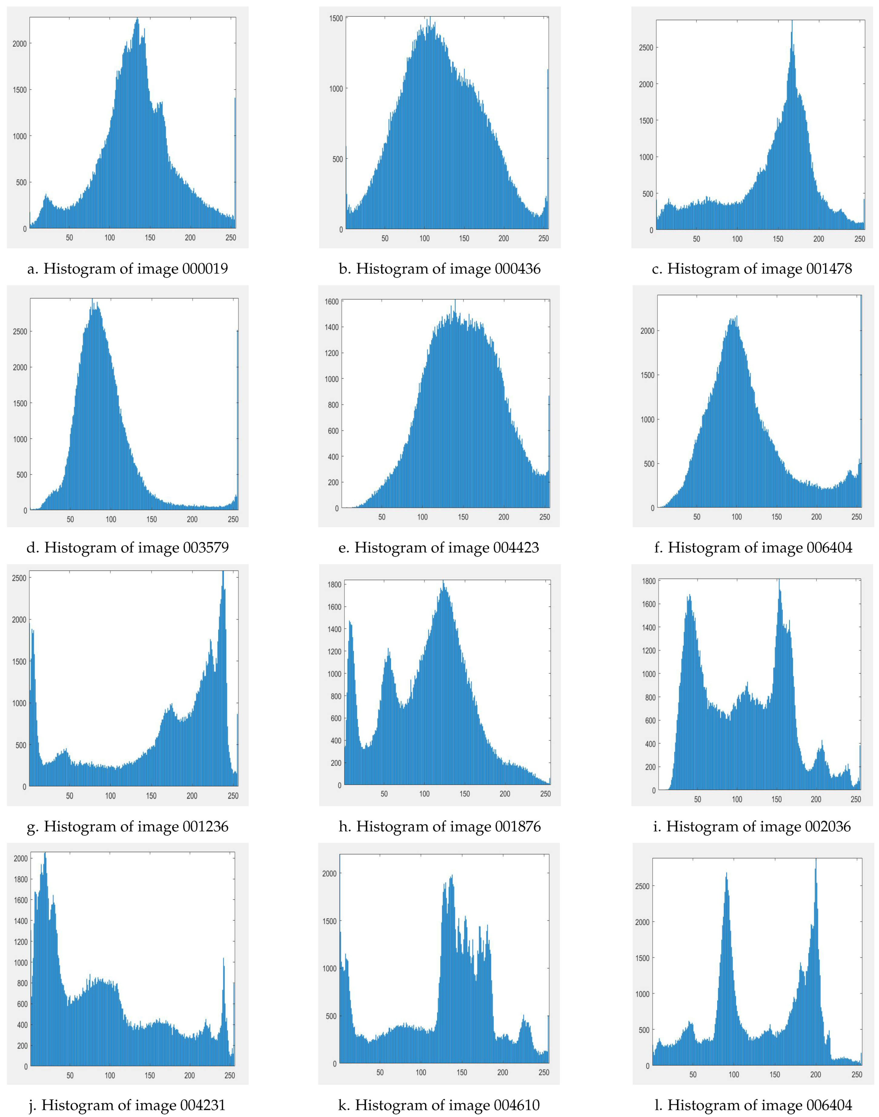
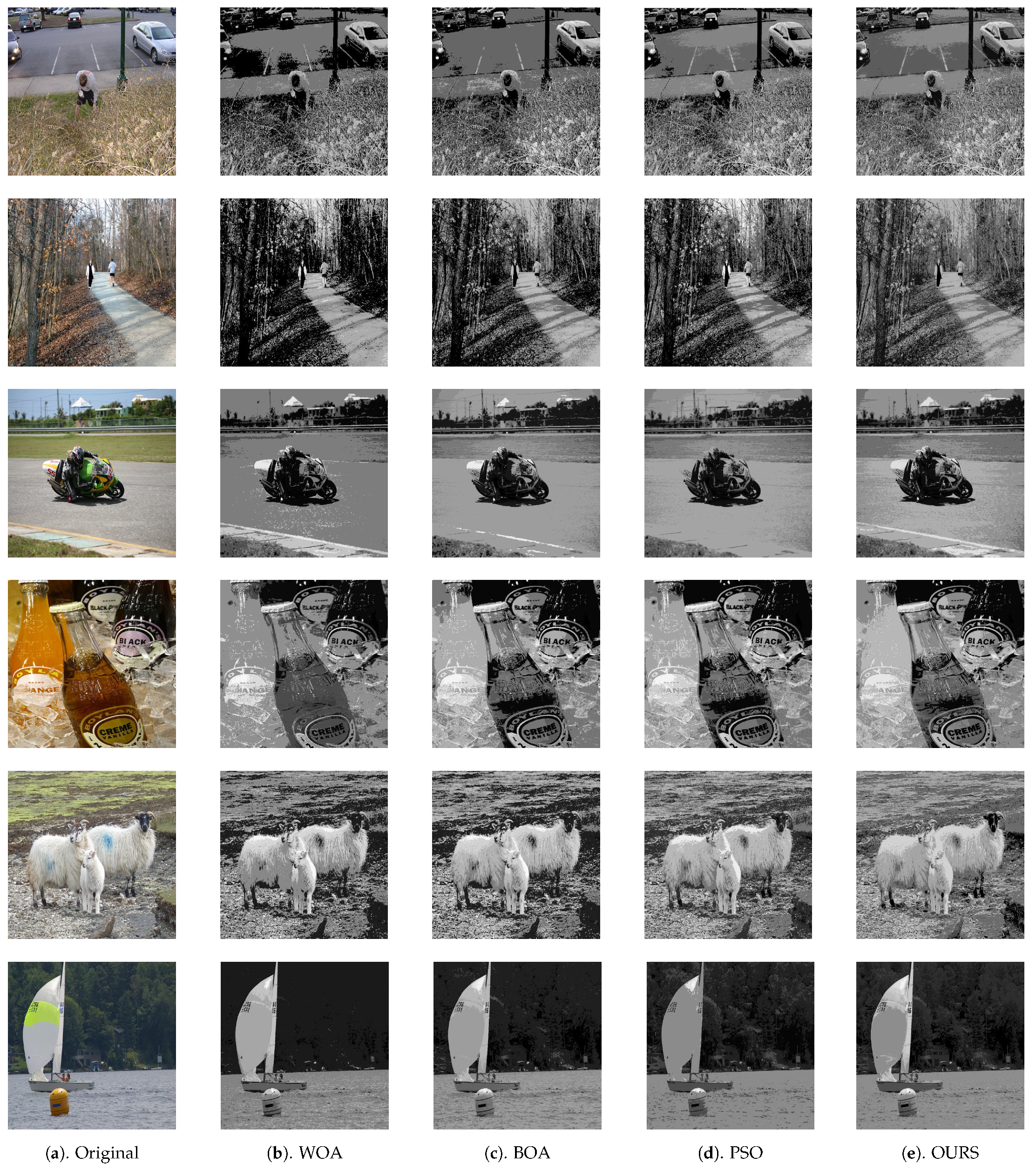
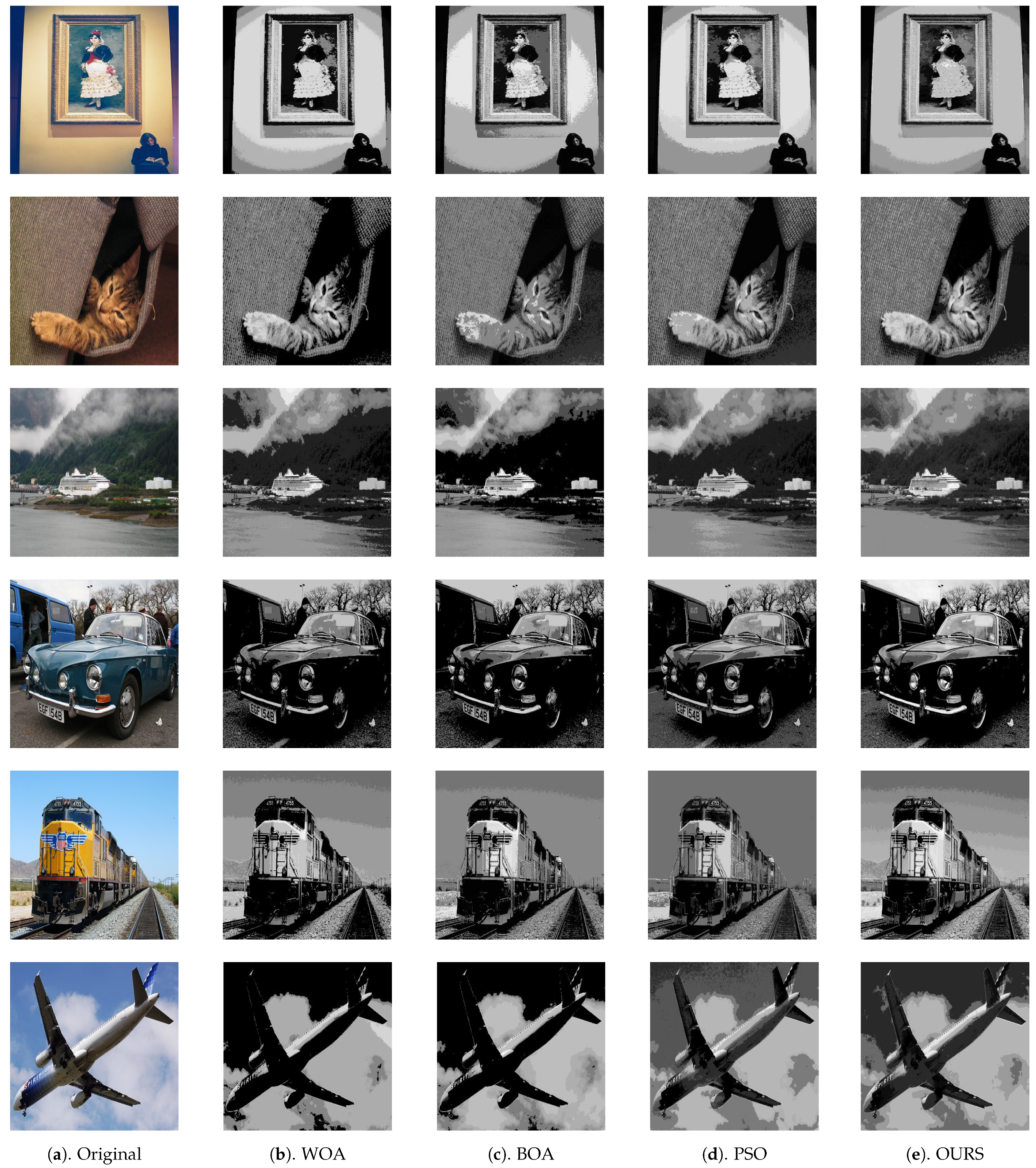
In this paper, the images in PASCAL 2012 [25] were selected as the experimental data set, including Figure 3a–f (numbered 000019, 000436, 001478, 003579, 004423, 006404). They were typical images with relatively centralized gray distribution and small inter class variance, while Figure 3g–l (numbered 001236, 001876, 002036, 004231, 004610, 006946) selected images with obvious differences in gray distribution, that is, the inter class variance was relatively large, as shown in Figure 3. Theoretically, the greater the number of segmentation thresholds, the greater the accuracy of the image segmentation. In order to quantitatively analyze the performance of segmentation, in the experiment, four groups of different segmentation thresholds were used. k is, 2, 4, 6, and 8 for index analysis. Our improved particle swarm optimization algorithm was compared with the classical particle swarm optimization algorithm [13], whale optimization algorithm [25], and butterfly optimization algorithm [26]. With several evaluation indicators, such as the classical particle swarm optimization algorithm, the whale optimization algorithm and the butterfly optimization algorithm are both bionic algorithms. The differences are that the whale optimization algorithm achieves the goal of searching by searching, surrounding, chasing, and attacking prey, while the butterfly algorithm locates the source of the target through its own perception. In this way, we can better understand the segmentation effect of the improved particle swarm optimization OTSU image segmentation method compared with other algorithms under different thresholds. Table 3, Table 4, Table 5, Table 6, Table 7, Table 8, Table 9 and Table 10 show the comparison results of PSNR, SSIM, FSIM, and fitness values, respectively. It can be seen that with the increase of the number of thresholds k, the distortion after image segmentation gradually decreases, which is closer to the original image. SSIM and FSIM gradually increase, and the segmentation performance gets better and better, which shows the advantages of multi-threshold image segmentation methods. To verify the universality of the algorithm in this paper, we randomly selected 100 images from the PASCAL 2012 dataset for the same experiment and listed the average values of the experimental parameters in Table 11. In addition, the algorithm that performs best on the evaluation criteria is marked in bold.
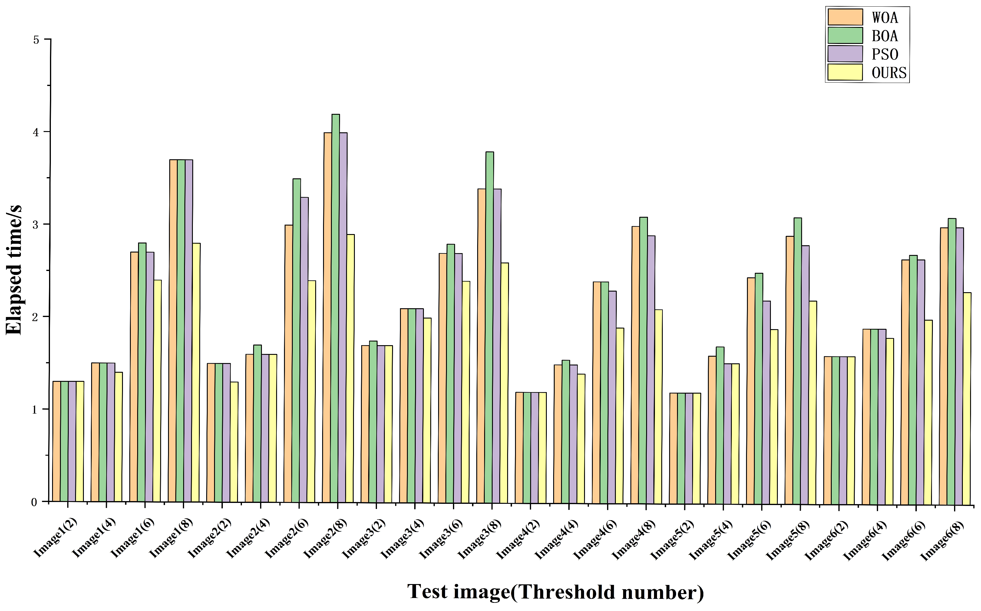
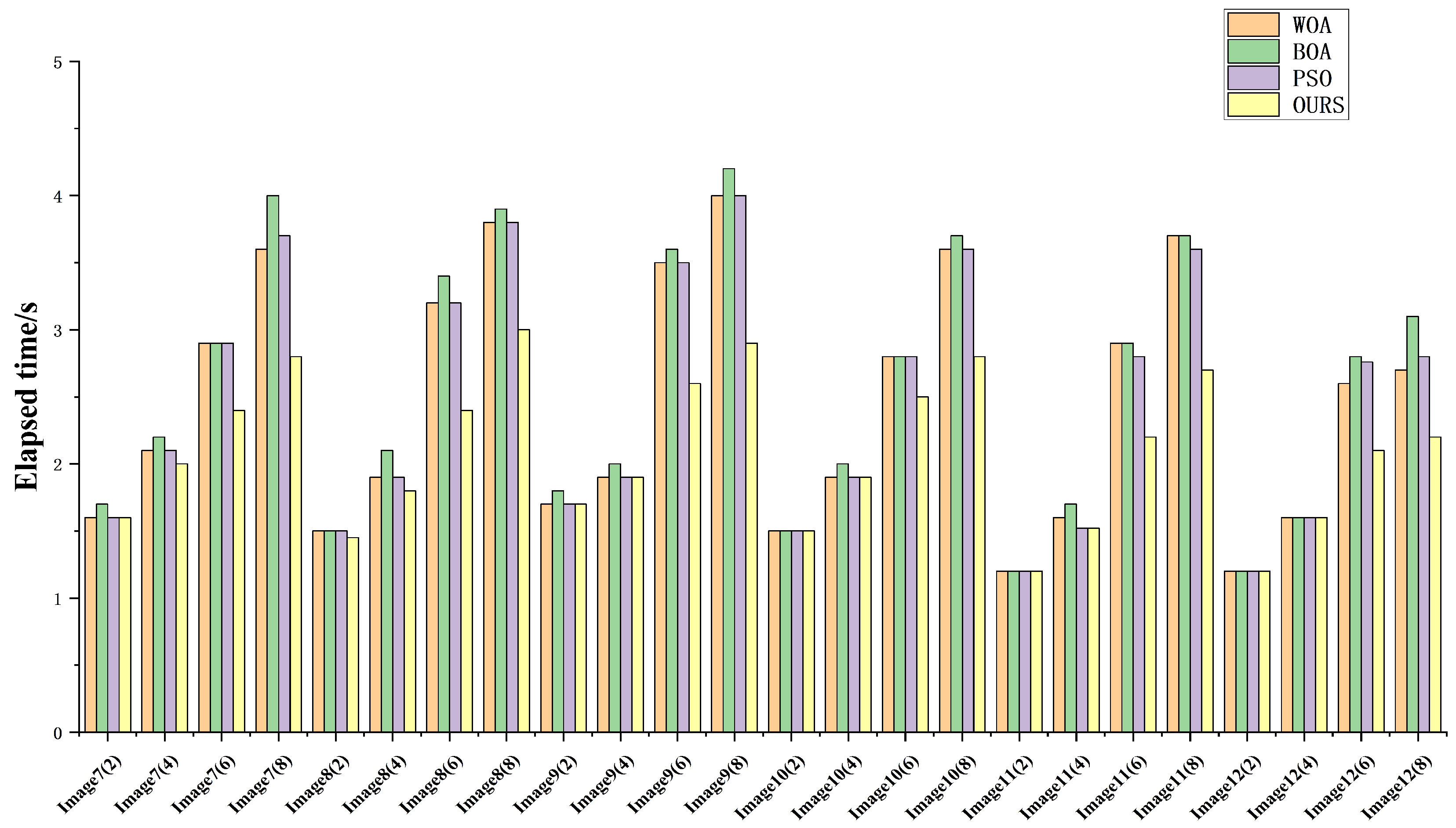
When the number of thresholds is small (k = 2 or k = 4), the PSNR, SSIM, and FSIM values of the improved particle swarm optimization algorithm are slightly better than other algorithms. However, after the threshold number increases (k = 6 or k = 8), the advantages of improved particle swarm optimization are reflected. The calculated PSNR, SSIM, and FSIM values were the highest among the four algorithms, which indicates that the segmentation, when the improved particle swarm algorithm solves the optimal threshold combination, has the highest similarity with the original image, and the optimization accuracy performance of the algorithm can be reflected. The algorithm runtime is shown in Figure 4 and Figure 5.
From Table 3, Table 4, Table 5, Table 6, Table 7, Table 8, Table 9 and Table 10, it can be seen that the segmentation effect of the proposed algorithm is better. Image 1 (000019) was selected as an example, and the PSNR value of the image, k = 8, was 21.3771, which was significantly better than other comparison algorithms. The SSIM value of the image was 0.7333, which was also slightly better than other algorithms, indicating that the image distortion is low and ensures the image quality after segmentation. Under the premise of maintaining the segmentation effect, it can be seen from Figure 4 that the running time of the proposed scheme was shorter than that of other algorithms, especially in the case of a large number of thresholds. When k = 8, the algorithm segmentation running time was shortened from 3.7 s to 2.8 s, which decreased by more than 30%, which greatly improved the running speed. To verify the universality of the algorithm in this paper, we randomly selected 100 images from the PASCAL 2012 dataset for parameter comparison tests. The experimental results show that our method ia faster and more accurate than other algorithms in terms of PSNR, SSIM, FSIM, and runtime parameters. Experimental results show that the proposed method can improve the segmentation accuracy and segmentation efficiency. Table 6 and Table 10 show the fitness values obtained by different algorithms under different thresholds. The segmented image is shown in Figure 6 and Figure 7.
6. Conclusions
This paper proposes an improved particle swarm optimization algorithm and applies it to the field of multi-threshold imaging. A new elite particle search strategy is introduced to narrow the scope of particle search, asynchronous monotone increasing social learning factor and asynchronous monotone decreasing individual learning factor are introduced to balance global and local search, and chaos optimization is introduced to increase population diversity. An optimal multi-threshold combination of image segmentation based on an improved particle swarm optimization algorithm is used for optimization, and multi-threshold image segmentation is realized. The test function proves that the algorithm has good development and exploration. The experimental results show that the proposed algorithm can achieve higher segmentation accuracy and efficiency.
Although our method has a faster speed and higher accuracy in image segmentation, compared with threshold segmentation methods, such as fuzzy entropy, our algorithm has a greater speed improvement, but the segmentation accuracy is slightly insufficient, which is one of the directions we will study in the future. Next, it is important to consider applying the improved particle swarm optimization algorithm to image segmentation and image processing in other fields (such as new material image processing, target detection, lightweight embedded robots, and other fields), study the ability of the algorithm to solve practical problems, and further enhance the practicability of the algorithm.
Author Contributions
Conceptualization, J.Z. (Jianfeng Zheng) and Y.G.; methodology, J.Z. (Jianfeng Zheng), Y.G. and Y.L.; software, Y.G.; validation, J.Z. (Jianfeng Zheng), Y.G. and J.Z. (Ji Zhang); formal analysis, Y.G. and H.Z.; investigation, Y.G. and Y.L.; resources, J.Z. (Jianfeng Zheng) and J.Z. (Ji Zhang); data curation, Y.G., Y.L. and H.Z.; writing—original draft preparation, Y.G.; writing—review and editing, J.Z. (Jianfeng Zheng) and Y.G.; visualization, Y.G.; supervision, J.Z. (Jianfeng Zheng) and J.Z. (Ji Zhang). All authors have read and agreed to the published version of the manuscript.
Funding
This research was funded by the Postgraduate Research & Practice Innovation Program of Jiangsu Province under the grant number [SJCX21_1282].
Institutional Review Board Statement
Not applicable.
Informed Consent Statement
Not applicable.
Data Availability Statement
Not applicable.
Conflicts of Interest
The authors declare no conflict of interest.
Abbreviations
The following abbreviations are used in this manuscript:
| PSO | Particle swarm algorithm |
| PSNR | Peak-Signal-to-Noise-Ratio |
| FSIM | Feature similarity |
| SSIM | Structural Similarity |
References
- Cheng, Y.; Li, B. Image Segmentation Technology and Its Application in Digital Image Processing. In Proceedings of the 2021 IEEE Asia-Pacific Conference on Image Processing, Electronics and Computers (IPEC), Dalian, China, 14–16 April 2021; pp. 1174–1177. [Google Scholar]
- Chakraborty, F.; Roy, P.K.; Nandi, D. Oppositional elephant herding optimization with dynamic Cauchy mutation for multilevel image thresholding. Evol. Intell. 2019, 12, 445–467. [Google Scholar]
- Abd Elaziz, M.; Oliva, D.; Ewees, A.A.; Xiong, S. Multi-level thresholding-based grey scale image segmentation using multi-objective multi-verse optimizer. Expert Syst. Appl. 2019, 125, 112–129. [Google Scholar]
- Upadhyay, P.; Chhabra, J.K. Kapur’s entropy based optimal multilevel image segmentation using crow search algorithm. Appl. Soft Comput. 2020, 97, 105522. [Google Scholar]
- Yazid, H.; Basah, S.N.; Rahim, S.A.; Safar, M.J.A.; Basaruddin, K.S. Performance analysis of entropy thresholding for successful image segmentation. Multimed. Tools Appl. 2022, 81, 6433–6450. [Google Scholar]
- Mahajan, S.; Mittal, N.; Pandit, A.K. Image segmentation using multilevel thresholding based on type II fuzzy entropy and marine predators algorithm. Multimed. Tools Appl. 2021, 80, 19335–19359. [Google Scholar] [CrossRef]
- Wu, B.; Zhou, J.; Ji, X.; Yin, Y.; Shen, X. An ameliorated teaching–learning-based optimization algorithm based study of image segmentation for multilevel thresholding using Kapur’s entropy and Otsu’s between class variance. Inf. Sci. 2020, 533, 72–107. [Google Scholar]
- Houssein, E.H.; Helmy, B.E.d.; Oliva, D.; Jangir, P.; Premkumar, M.; Elngar, A.A.; Shaban, H. An efficient multi-thresholding based COVID-19 CT images segmentation approach using an improved equilibrium optimizer. Biomed. Signal Process. Control 2022, 73, 103401. [Google Scholar]
- Sharma, S.; Saha, A.K.; Majumder, A.; Nama, S. MPBOA—A novel hybrid butterfly optimization algorithm with symbiosis organisms search for global optimization and image segmentation. Multimed. Tools Appl. 2021, 80, 12035–12076. [Google Scholar]
- Elaziz, M.E.A.; Heidari, A.A.; Fujita, H.; Moayedi, H. A competitive chain-based Harris Hawks Optimizer for global optimization and multi-level image thresholding problems. Appl. Soft Comput. 2020, 95, 106347. [Google Scholar] [CrossRef]
- Zhang, L.; Wang, J.; An, Z. FCM fuzzy clustering image segmentation algorithm based on fractional particle swarm optimization. J. Intell. Fuzzy Syst. 2020, 38, 3575–3584. [Google Scholar]
- Zhao, D.; Liu, L.; Yu, F.; Heidari, A.A.; Wang, M.; Oliva, D.; Muhammad, K.; Chen, H. Ant colony optimization with horizontal and vertical crossover search: Fundamental visions for multi-threshold image segmentation. Expert Syst. Appl. 2021, 167, 114122. [Google Scholar] [CrossRef]
- Holland, J.H. Adaptation in Natural and Artificial Systems: An Introductory Analysis with Applications to Biology, Control, and Artificial Intelligence; MIT Press: Cambridge, MA, USA, 1992. [Google Scholar]
- Shami, T.M.; El-Saleh, A.A.; Alswaitti, M.; Al-Tashi, Q.; Summakieh, M.A.; Mirjalili, S. Particle swarm optimization: A comprehensive survey. IEEE Access 2022, 10, 10031–10061. [Google Scholar] [CrossRef]
- Raj, S.; Bhattacharyya, B. Optimal placement of TCSC and SVC for reactive power planning using Whale optimization algorithm. Swarm Evol. Comput. 2018, 40, 131–143. [Google Scholar]
- Shiva, C.K.; Gudadappanavar, S.S.; Vedik, B.; Babu, R.; Raj, S.; Bhattacharyya, B. Fuzzy-Based Shunt VAR Source Placement and Sizing by Oppositional Crow Search Algorithm. J. Control. Autom. Electr. Syst. 2022, 33, 1576–1591. [Google Scholar]
- Babu, R.; Kumar, V.; Shiva, C.K.; Raj, S.; Bhattacharyya, B. Application of Sine–Cosine Optimization Algorithm for Minimization of Transmission Loss. Technol. Econ. Smart Grids Sustain. Energy 2022, 7, 6. [Google Scholar] [CrossRef]
- Heidari, A.A.; Mirjalili, S.; Faris, H.; Aljarah, I.; Mafarja, M.; Chen, H. Harris hawks optimization: Algorithm and applications. Future Gener. Comput. Syst. 2019, 97, 849–872. [Google Scholar] [CrossRef]
- Su, H.; Zhao, D.; Yu, F.; Heidari, A.A.; Zhang, Y.; Chen, H.; Li, C.; Pan, J.; Quan, S. Horizontal and vertical search artificial bee colony for image segmentation of COVID-19 X-ray images. Comput. Biol. Med. 2022, 142, 105181. [Google Scholar] [CrossRef] [PubMed]
- Xu, B.; Heidari, A.A.; Kuang, F.; Zhang, S.; Chen, H.; Cai, Z. Quantum Nelder-Mead Hunger Games Search for optimizing photovoltaic solar cells. Int. J. Energy Res. 2022, 46, 12417–12466. [Google Scholar]
- Trojovskỳ, P.; Dehghani, M. Pelican optimization algorithm: A novel nature-inspired algorithm for engineering applications. Sensors 2022, 22, 855. [Google Scholar] [CrossRef] [PubMed]
- Shabani, A.; Asgarian, B.; Gharebaghi, S.A.; Salido, M.A.; Giret, A. A new optimization algorithm based on search and rescue operations. Math. Probl. Eng. 2019, 2019, 2482543. [Google Scholar] [CrossRef]
- Oliva, D.; Elaziz, M.A. An improved brainstorm optimization using chaotic opposite-based learning with disruption operator for global optimization and feature selection. Soft Comput. 2020, 24, 14051–14072. [Google Scholar] [CrossRef]
- Sun, Y.; Yang, Y. An Adaptive Bi-Mutation-Based Differential Evolution Algorithm for Multi-Threshold Image Segmentation. Appl. Sci. 2022, 12, 5759. [Google Scholar]
- Shetty, S. Application of convolutional neural network for image classification on Pascal VOC challenge 2012 dataset. arXiv 2016, arXiv:1607.03785. [Google Scholar]
- Liang, J.J.; Suganthan, P.N.; Deb, K. Novel composition test functions for numerical global optimization. In Proceedings of the 2005 IEEE Swarm Intelligence Symposium, SIS 2005, Pasadena, CA, USA, 8–10 June 2005; pp. 68–75. [Google Scholar]
- Mirjalili, S.; Lewis, A. The whale optimization algorithm. Adv. Eng. Softw. 2016, 95, 51–67. [Google Scholar]
- Arora, S.; Singh, S. Butterfly optimization algorithm: A novel approach for global optimization. Soft Comput. 2019, 23, 715–734. [Google Scholar]
- Huynh-Thu, Q.; Ghanbari, M. Scope of validity of PSNR in image/video quality assessment. Electron. Lett. 2008, 44, 800–801. [Google Scholar]
- Hore, A.; Ziou, D. Image quality metrics: PSNR vs. SSIM. In Proceedings of the 2010 IEEE 20th International Conference on Pattern Recognition, Istanbul, Turkey, 23–26 August 2010; pp. 2366–2369. [Google Scholar]
- Wang, Z.; Bovik, A.C.; Sheikh, H.R.; Simoncelli, E.P. Image quality assessment: From error visibility to structural similarity. IEEE Trans. Image Process. 2004, 13, 600–612. [Google Scholar]
- Brunet, D.; Vrscay, E.R.; Wang, Z. On the mathematical properties of the structural similarity index. IEEE Trans. Image Process. 2011, 21, 1488–1499. [Google Scholar] [CrossRef] [PubMed]
- Sara, U.; Akter, M.; Uddin, M.S. Image quality assessment through FSIM, SSIM, MSE and PSNR—A comparative study. J. Comput. Commun. 2019, 7, 8–18. [Google Scholar] [CrossRef] [Green Version]
- Zhang, L.; Zhang, L.; Mou, X.; Zhang, D. FSIM: A feature similarity index for image quality assessment. IEEE Trans. Image Process. 2011, 20, 2378–2386. [Google Scholar]
Figure 1.
Particle swarm narrows the search range according to the contribution of particles.

Figure 2.
Improved particle swarm algorithm flowchart.

Figure 3.
Histogram distribution.

Figure 4.
Algorithm running time (Images a–f in Figure 3).
Figure 4.
Algorithm running time (Images a–f in Figure 3).

Figure 5.
Algorithm running time (Images g–l in Figure 3).
Figure 5.
Algorithm running time (Images g–l in Figure 3).

Figure 6.
When threshold , the original image and the segmented image of different algorithms are shown (images a–f in Figure 3).
Figure 6.
When threshold , the original image and the segmented image of different algorithms are shown (images a–f in Figure 3).

Figure 7.
When threshold , the original image and the segmented image of different algorithms are shown (images g–l in Figure 3).
Figure 7.
When threshold , the original image and the segmented image of different algorithms are shown (images g–l in Figure 3).


Table 1.
Benchmark Function.
| Test Function | Type | Dim | Range | |
|---|---|---|---|---|
| = | US | 30 | 0 | |
| = | US | 30 | 0 | |
| = | US | 30 | 0 | |
| = | US | 30 | 0 | |
| = | UN | 30 | 0 | |
| = | UN | 30 | 0 | |
| = | UN | 30 | 0 | |
| = | UN | 30 | 0 | |
| = | FDM | 2 | ||
| = | FDM | 2 | 0.398 | |
| = | FDM | 2 | 3 | |
| = | FDM | 4 | [0,10] |
Table 2.
Compare the mean and variance of different algorithms through benchmark functions.
| Function | Mean (WOA) | Std (WOA) | Mean (BOA) | Std (BOA) | Mean (PSO) | Std (PSO) | Mean (OURS) | Std (OURS) |
|---|---|---|---|---|---|---|---|---|
| 0 | 0 | 0 | 0 | 0 | 0 | |||
| 0 | 0 | 0 | 0 | 0.23241 | 0 | 0 | ||
| 0 | 0 | 0.43910 | 0.18334 | 5.61222 | 0.73845 | 0 | 0 | |
| 0.00511 | 0.00429 | 0.00935 | 0.00903 | 0.69190 | 0.21219 | 0.00149 | 0.00065 | |
| 0 | 0 | 0 | 0 | 2.10830 | 0.27572 | 0 | 0 | |
| 0 | 0 | 0 | 0 | 0.00105 | 0.00168 | 0 | 0 | |
| 0.02203 | 0.01070 | 0.69756 | 0.08152 | 4.41429 | 1.81612 | 0.03898 | 0.07815 | |
| 0 | 0 | 0.01205 | 0.01832 | 0.50179 | 0.24452 | 0 | 0 | |
| 0 | N\A | N\A | 0 | 0 | ||||
| 0.39790 | 0.54290 | 0.30599 | 0.39789 | 0 | 0.39789 | |||
| 3.00001 | 3.04893 | 0.05603 | 3 | 0 | 3.00017 | 0.00025 | ||
| 3.34554 | 0.38772 | 3.24476 | 0.12228 |
Table 3.
Comparison of PSNR in images a–f.
| Metric Name | Image | k | WOA | BOA | PSO | OURS |
|---|---|---|---|---|---|---|
| PSNR | Image1(000019) | 2 | 11.4924 | 12.6732 | 13.0284 | 13.7823 |
| 4 | 12.5075 | 13.7829 | 14.1673 | 14.7642 | ||
| 6 | 16.5389 | 17.2659 | 17.8454 | 19.6037 | ||
| 8 | 19.8595 | 20.4863 | 20.5269 | 21.3771 | ||
| Image2(000436) | 2 | 13.1415 | 13.7986 | 14.5376 | 14.1383 | |
| 4 | 14.1361 | 14.5284 | 15.3228 | 15.6705 | ||
| 6 | 17.9243 | 17.9988 | 18.3650 | 19.3411 | ||
| 8 | 18.5029 | 19.2229 | 20.9130 | 21.9703 | ||
| Image3(001478) | 2 | 13.3784 | 13.7194 | 13.7913 | 14.2379 | |
| 4 | 13.6647 | 14.1434 | 14.9181 | 15.4509 | ||
| 6 | 15.8758 | 16.4661 | 17.4344 | 18.6340 | ||
| 8 | 17.3109 | 17.6060 | 19.4388 | 20.3651 | ||
| Image4(003579) | 2 | 13.6386 | 13.5726 | 14.4871 | 15.9936 | |
| 4 | 14.3408 | 14.7052 | 15.6358 | 15.7378 | ||
| 6 | 15.9297 | 16.6595 | 17.2260 | 18.2881 | ||
| 8 | 16.6926 | 16.8525 | 17.4432 | 19.6017 | ||
| Image5(004423) | 2 | 15.1932 | 15.8189 | 15.5466 | 15.7275 | |
| 4 | 15.5115 | 16.2379 | 16.9289 | 16.8156 | ||
| 6 | 17.5728 | 18.8819 | 20.8917 | 21.7370 | ||
| 8 | 18.6900 | 19.9407 | 21.9854 | 23.3966 | ||
| Image6(006404) | 2 | 13.8768 | 13.8550 | 14.9768 | 14.9706 | |
| 4 | 14.6173 | 14.7452 | 14.8361 | 15.7539 | ||
| 6 | 16.5043 | 17.5922 | 18.7453 | 19.1893 | ||
| 8 | 17.8543 | 18.5252 | 20.7008 | 21.1228 |
Table 4.
Comparison of SSIM in images a–f.
| Metric Name | Image | k | WOA | BOA | PSO | OURS |
|---|---|---|---|---|---|---|
| SSIM | Image1(000019) | 2 | 0.4186 | 0.4628 | 0.4521 | 0.4955 |
| 4 | 0.4447 | 0.4559 | 0.5443 | 0.5968 | ||
| 6 | 0.4921 | 0.5161 | 0.6220 | 0.6973 | ||
| 8 | 0.6899 | 0.6930 | 0.7011 | 0.7333 | ||
| Image2(000436) | 2 | 0.4336 | 0.4922 | 0.5550 | 0.5806 | |
| 4 | 0.4781 | 0.5615 | 0.5975 | 0.6381 | ||
| 6 | 0.5482 | 0.6102 | 0.6238 | 0.6676 | ||
| 8 | 0.5720 | 0.6267 | 0.6541 | 0.7895 | ||
| Image3(001478) | 2 | 0.4299 | 0.4474 | 0.5120 | 0.5506 | |
| 4 | 0.5219 | 0.5774 | 0.6484 | 0.6386 | ||
| 6 | 0.5634 | 0.5971 | 0.6960 | 0.7235 | ||
| 8 | 0.6563 | 0.6857 | 0.7436 | 0.8154 | ||
| Image4(003579) | 2 | 0.5610 | 0.5961 | 0.5969 | 0.5904 | |
| 4 | 0.5796 | 0.6057 | 0.6172 | 0.6714 | ||
| 6 | 0.6286 | 0.6411 | 0.6484 | 0.7172 | ||
| 8 | 0.6764 | 0.6938 | 0.7036 | 0.7297 | ||
| Image5(004423) | 2 | 0.3469 | 0.3755 | 0.3758 | 0.4954 | |
| 4 | 0.4443 | 0.4570 | 0.5714 | 0.5978 | ||
| 6 | 0.5396 | 0.5680 | 0.6687 | 0.7178 | ||
| 8 | 0.6817 | 0.6638 | 0.7430 | 0.7746 | ||
| Image6(006404) | 2 | 0.4216 | 0.4419 | 0.4675 | 0.4990 | |
| 4 | 0.4429 | 0.4723 | 0.5482 | 0.5745 | ||
| 6 | 0.4859 | 0.5186 | 0.5744 | 0.6482 | ||
| 8 | 0.5632 | 0.6114 | 0.6367 | 0.6861 |
Table 5.
Comparison of FSIM in images a–f.
| Metric Name | Image | k | WOA | BOA | PSO | OURS |
|---|---|---|---|---|---|---|
| FSIM | Image1(000019) | 2 | 0.7053 | 0.7214 | 0.7423 | 0.7711 |
| 4 | 0.7278 | 0.7535 | 0.7861 | 0.8026 | ||
| 6 | 0.7596 | 0.7974 | 0.8013 | 0.8250 | ||
| 8 | 0.8058 | 0.8144 | 0.8224 | 0.8476 | ||
| Image2(000436) | 2 | 0.6525 | 0.6934 | 0.7571 | 0.7918 | |
| 4 | 0.7120 | 0.7235 | 0.7610 | 0.8132 | ||
| 6 | 0.7350 | 0.7441 | 0.7832 | 0.8317 | ||
| 8 | 0.7582 | 0.7655 | 0.8086 | 0.8594 | ||
| Image3(001478) | 2 | 0.6592 | 0.6763 | 0.7084 | 0.7135 | |
| 4 | 0.6795 | 0.6940 | 0.7288 | 0.7402 | ||
| 6 | 0.7110 | 0.7417 | 0.7643 | 0.7732 | ||
| 8 | 0.7390 | 0.7652 | 0.7864 | 0.8277 | ||
| Image4(003579) | 2 | 0.7495 | 0.7634 | 0.7770 | 0.7953 | |
| 4 | 0.7679 | 0.7855 | 0.7921 | 0.8113 | ||
| 6 | 0.7869 | 0.8024 | 0.8275 | 0.8322 | ||
| 8 | 0.8139 | 0.8289 | 0.8411 | 0.8672 | ||
| Image5(004423) | 2 | 0.7552 | 0.7695 | 0.7892 | 0.7859 | |
| 4 | 0.7723 | 0.7820 | 0.8118 | 0.8382 | ||
| 6 | 0.7965 | 0.7998 | 0.8367 | 0.8547 | ||
| 8 | 0.8185 | 0.8247 | 0.8559 | 0.8712 | ||
| Image6(006404) | 2 | 0.6292 | 0.6467 | 0.6638 | 0.6779 | |
| 4 | 0.6482 | 0.6614 | 0.6735 | 0.7066 | ||
| 6 | 0.6684 | 0.6876 | 0.6910 | 0.7134 | ||
| 8 | 0.6835 | 0.7155 | 0.7334 | 0.7780 |
Table 6.
Comparison of Fitness in images a–f.
| Metric Name | Image | k | WOA | BOA | PSO | OURS |
|---|---|---|---|---|---|---|
| Fitness | Image1(000019) | 2 | 1704.8574 | 1704.5298 | 1704.3760 | 1704.8259 |
| 4 | 2539.6813 | 2539.4239 | 2539.2458 | 2539.7578 | ||
| 6 | 2765.9773 | 2765.2783 | 2764.2456 | 2764.2568 | ||
| 8 | 3858.8308 | 3858.1415 | 3857.7672 | 3858.3303 | ||
| Image2(000436) | 2 | 2213.5065 | 2213.1738 | 2213.3147 | 2213.1353 | |
| 4 | 3450.9044 | 3450.6474 | 3450.6818 | 3450.8937 | ||
| 6 | 4033.8449 | 4033.1927 | 4033.1099 | 4033.8446 | ||
| 8 | 4905.7727 | 4905.6214 | 4904.3492 | 4905.7649 | ||
| Image3(001478) | 2 | 2451.9890 | 2451.7517 | 2451.1717 | 2451.9397 | |
| 4 | 3375.8902 | 3375.4263 | 3375.1152 | 3375.8437 | ||
| 6 | 3766.7624 | 3766.2709 | 3766.2389 | 3766.4151 | ||
| 8 | 3986.8089 | 3986.3177 | 3984.3164 | 3986.7295 | ||
| Image4(003579) | 2 | 1765.9298 | 1765.3507 | 1765.1458 | 1765.4344 | |
| 4 | 2276.9954 | 2276.8173 | 2276.3680 | 2276.9576 | ||
| 6 | 3877.9674 | 3877.1473 | 3877.1218 | 3877.2627 | ||
| 8 | 5090.7653 | 5090.5032 | 5090.2623 | 5090.6338 | ||
| Image5(004423) | 2 | 1721.8701 | 1721.1817 | 1721.1124 | 1721.2721 | |
| 4 | 2551.9400 | 2551.7442 | 2551.4594 | 2551.8431 | ||
| 6 | 2968.9682 | 2968.7638 | 2968.4520 | 2968.7339 | ||
| 8 | 3859.5790 | 3859.1403 | 3857.1300 | 3859.3798 | ||
| Image6(006404) | 2 | 2972.7388 | 2972.2542 | 2972.1044 | 2972.4020 | |
| 4 | 3387.7543 | 3387.3168 | 3387.2231 | 3387.6870 | ||
| 6 | 4142.6126 | 4142.4051 | 4142.3022 | 4142.4612 | ||
| 8 | 5984.9055 | 5984.7659 | 5984.3470 | 5984.8045 |
Table 7.
Comparison of PSNR in Images g–l.
| Metric Name | Image | k | WOA | BOA | PSO | OURS |
|---|---|---|---|---|---|---|
| PSNR | Image7(001236) | 2 | 13.8293 | 14.5503 | 15.7167 | 15.7977 |
| 4 | 14.1970 | 14.6582 | 15.6621 | 15.6767 | ||
| 6 | 17.4146 | 17.5859 | 18.3812 | 20.5188 | ||
| 8 | 18.2980 | 18.1377 | 19.1016 | 21.6592 | ||
| Image8(001876) | 2 | 13.4009 | 14.5790 | 14.8465 | 14.7751 | |
| 4 | 14.5690 | 15.6121 | 15.6524 | 16.4362 | ||
| 6 | 16.4996 | 16.7998 | 17.5997 | 19.7598 | ||
| 8 | 17.9384 | 18.6226 | 19.5498 | 21.5051 | ||
| Image9(002036) | 2 | 13.5557 | 14.4696 | 14.6034 | 14.7418 | |
| 4 | 15.5611 | 15.1427 | 16.4177 | 16.3583 | ||
| 6 | 16.5306 | 17.3650 | 18.3565 | 19.1878 | ||
| 8 | 18.4281 | 18.5254 | 20.5951 | 22.6777 | ||
| Image10(004231) | 2 | 13.6632 | 14.3337 | 15.2033 | 15.9469 | |
| 4 | 14.2989 | 14.6908 | 15.5551 | 15.2502 | ||
| 6 | 15.1205 | 16.5671 | 16.7517 | 17.4736 | ||
| 8 | 15.7529 | 16.7325 | 17.2486 | 18.2805 | ||
| Image11(004610) | 2 | 14.7697 | 14.9273 | 15.6025 | 16.4122 | |
| 4 | 14.8004 | 15.4323 | 15.8120 | 16.9533 | ||
| 6 | 16.1080 | 17.5817 | 19.8235 | 20.4539 | ||
| 8 | 18.6965 | 19.8851 | 20.8712 | 21.7442 | ||
| Image12(006946) | 2 | 11.6113 | 12.9387 | 13.8889 | 13.3067 | |
| 4 | 12.3074 | 12.4025 | 14.6690 | 14.1064 | ||
| 6 | 15.1121 | 15.2394 | 16.3323 | 17.7174 | ||
| 8 | 16.7195 | 16.8900 | 17.9451 | 18.3580 |
Table 8.
Comparison of SSIM in Images g–l.
| Metric Name | Image | k | WOA | BOA | PSO | OURS |
|---|---|---|---|---|---|---|
| SSIM | Image7(001236) | 2 | 0.5571 | 0.5861 | 0.5875 | 0.6273 |
| 4 | 0.6012 | 0.6302 | 0.6561 | 0.6567 | ||
| 6 | 0.6231 | 0.6519 | 0.7253 | 0.7461 | ||
| 8 | 0.6685 | 0.6918 | 0.7335 | 0.7824 | ||
| Image8(001876) | 2 | 0.4474 | 0.4610 | 0.4619 | 0.4849 | |
| 4 | 0.4971 | 0.5300 | 0.5719 | 0.5826 | ||
| 6 | 0.5496 | 0.5826 | 0.6138 | 0.6611 | ||
| 8 | 0.6215 | 0.6291 | 0.6736 | 0.6884 | ||
| Image9(002036) | 2 | 0.3660 | 0.3920 | 0.4136 | 0.4650 | |
| 4 | 0.3878 | 0.4012 | 0.4896 | 0.5109 | ||
| 6 | 0.4127 | 0.4322 | 0.5483 | 0.5705 | ||
| 8 | 0.4818 | 0.4845 | 0.5912 | 0.6318 | ||
| Image10(004231) | 2 | 0.3309 | 0.3387 | 0.3567 | 0.3671 | |
| 4 | 0.3726 | 0.3862 | 0.4269 | 0.4262 | ||
| 6 | 0.4245 | 0.4527 | 0.4565 | 0.5049 | ||
| 8 | 0.4708 | 0.5428 | 0.5565 | 0.5778 | ||
| Image11(004610) | 2 | 0.6188 | 0.6238 | 0.6454 | 0.6840 | |
| 4 | 0.6297 | 0.6632 | 0.6925 | 0.6918 | ||
| 6 | 0.7249 | 0.7650 | 0.7693 | 0.7891 | ||
| 8 | 0.7368 | 0.7728 | 0.7881 | 0.8017 | ||
| Image12(006946) | 2 | 0.4310 | 0.4429 | 0.4523 | 0.5013 | |
| 4 | 0.4984 | 0.5204 | 0.5363 | 0.5699 | ||
| 6 | 0.5377 | 0.6239 | 0.6737 | 0.6875 | ||
| 8 | 0.6507 | 0.6918 | 0.7303 | 0.7471 |
Table 9.
Comparison of FSIM in Images g–l.
| Metric Name | Image | k | WOA | BOA | PSO | OURS |
|---|---|---|---|---|---|---|
| FSIM | Image7(001236) | 2 | 0.7066 | 0.7277 | 0.7510 | 0.7889 |
| 4 | 0.7397 | 0.7645 | 0.7916 | 0.8246 | ||
| 6 | 0.7560 | 0.8089 | 0.8433 | 0.8760 | ||
| 8 | 0.8030 | 0.8279 | 0.8660 | 0.8982 | ||
| Image8(001876) | 2 | 0.6461 | 0.6516 | 0.6747 | 0.6850 | |
| 4 | 0.6642 | 0.6737 | 0.6927 | 0.7071 | ||
| 6 | 0.6823 | 0.6957 | 0.7182 | 0.7419 | ||
| 8 | 0.7128 | 0.7246 | 0.7584 | 0.8142 | ||
| Image9(002036) | 2 | 0.6726 | 0.6949 | 0.7191 | 0.7347 | |
| 4 | 0.6938 | 0.7144 | 0.7341 | 0.7694 | ||
| 6 | 0.7220 | 0.7379 | 0.7550 | 0.7977 | ||
| 8 | 0.7421 | 0.7518 | 0.7796 | 0.8084 | ||
| Image10(004231) | 2 | 0.6381 | 0.6679 | 0.6980 | 0.7130 | |
| 4 | 0.6526 | 0.6729 | 0.7111 | 0.7368 | ||
| 6 | 0.6932 | 0.7274 | 0.7510 | 0.7787 | ||
| 8 | 0.7349 | 0.7564 | 0.7860 | 0.8072 | ||
| Image11(004610) | 2 | 0.7283 | 0.7484 | 0.7585 | 0.7467 | |
| 4 | 0.7379 | 0.7513 | 0.7685 | 0.7760 | ||
| 6 | 0.7451 | 0.7710 | 0.7819 | 0.8029 | ||
| 8 | 0.7670 | 0.7850 | 0.8129 | 0.8558 | ||
| Image12(006946) | 2 | 0.7375 | 0.7582 | 0.7955 | 0.8250 | |
| 4 | 0.7541 | 0.7763 | 0.8152 | 0.8430 | ||
| 6 | 0.7796 | 0.8097 | 0.8421 | 0.8654 | ||
| 8 | 0.8016 | 0.8217 | 0.8427 | 0.8693 |
Table 10.
Comparison of Fitness in Images g–l.
| Metric Name | Image | k | WOA | BOA | PSO | OURS |
|---|---|---|---|---|---|---|
| Fitness | Image7(001236) | 2 | 2750.8992 | 2750.7616 | 2750.1240 | 2750.7641 |
| 4 | 3517.7437 | 3517.7256 | 3517.3212 | 3517.7290 | ||
| 6 | 4509.9853 | 4509.7814 | 4509.5764 | 4509.7829 | ||
| 8 | 6495.5661 | 6495.5018 | 6493.2953 | 6495.5538 | ||
| Image8(001876) | 2 | 2338.4961 | 2338.3209 | 2338.2888 | 2338.4402 | |
| 4 | 3251.9846 | 3251.4460 | 3251.2548 | 3251.7075 | ||
| 6 | 3637.9811 | 3637.4199 | 3637.1219 | 3637.6122 | ||
| 8 | 4735.8050 | 4735.3475 | 4734.1491 | 4735.5701 | ||
| Image9(002036) | 2 | 2777.9633 | 2777.8345 | 2777.1929 | 2777.9091 | |
| 4 | 3709.8962 | 3709.2028 | 3709.1977 | 3709.6104 | ||
| 6 | 4837.6270 | 4837.2012 | 4837.1285 | 4837.5268 | ||
| 8 | 5453.6888 | 5453.5749 | 5453.3442 | 5453.6073 | ||
| Image10(004231) | 2 | 1699.8490 | 1699.3038 | 1699.1601 | 1699.7288 | |
| 4 | 2878.5953 | 2878.2350 | 2878.1299 | 2878.2976 | ||
| 6 | 3708.6870 | 3708.4114 | 3708.4016 | 3708.4181 | ||
| 8 | 4828.7905 | 4828.5773 | 4825.4886 | 4828.9096 | ||
| Image11(004610) | 2 | 1343.9485 | 1343.6048 | 1343.4410 | 1343.7570 | |
| 4 | 2561.8768 | 2561.4219 | 2561.3565 | 2561.2494 | ||
| 6 | 2905.9755 | 2905.5645 | 2905.5418 | 2905.7108 | ||
| 8 | 4101.8497 | 4101.5807 | 4100.4235 | 4101.6487 | ||
| Image12(006946) | 2 | 2200.6262 | 2200.1469 | 2200.1288 | 2200.5102 | |
| 4 | 3164.7962 | 3164.2352 | 3164.2936 | 3164.7918 | ||
| 6 | 3932.8209 | 3932.2591 | 3932.2245 | 3932.3805 | ||
| 8 | 4459.9945 | 4459.8215 | 4458.1837 | 4459.9166 |
Table 11.
Average of 100 image segmentation results.
| Metric Name | k | WOA | BOA | PSO | OURS |
|---|---|---|---|---|---|
| PSNR | 2 | 13.2343 | 14.7236 | 14.9630 | 15.8237 |
| 4 | 14.5273 | 14.9263 | 15.4328 | 15.9417 | |
| 6 | 16.3862 | 16.9732 | 17.7237 | 19.6872 | |
| 8 | 18.4687 | 19.2433 | 20.2934 | 21.6278 | |
| SSIM | 2 | 0.4327 | 0.4938 | 0.5019 | 0.5823 |
| 4 | 0.4825 | 0.5349 | 0.5835 | 0.6132 | |
| 6 | 0.5926 | 0.6419 | 0.6723 | 0.6835 | |
| 8 | 0.6324 | 0.6638 | 0.6924 | 0.7247 | |
| FSIM | 2 | 0.6842 | 0.7154 | 0.7369 | 0.7437 |
| 4 | 0.7147 | 0.7519 | 0.7830 | 0.8039 | |
| 6 | 0.7422 | 0.7751 | 0.7984 | 0.8241 | |
| 8 | 0.7645 | 0.7957 | 0.8226 | 0.8469 | |
| Running Tinme | 2 | 1.35 | 1.35 | 1.35 | 1.28 |
| 4 | 1.64 | 1.65 | 1.64 | 1.52 | |
| 6 | 2.85 | 3.12 | 2.97 | 2.25 | |
| 8 | 3.82 | 4.83 | 3.94 | 2.46 |
Publisher’s Note: MDPI stays neutral with regard to jurisdictional claims in published maps and institutional affiliations. |
© 2022 by the authors. Licensee MDPI, Basel, Switzerland. This article is an open access article distributed under the terms and conditions of the Creative Commons Attribution (CC BY) license (https://creativecommons.org/licenses/by/4.0/).
Share and Cite
MDPI and ACS Style
Zheng, J.; Gao, Y.; Zhang, H.; Lei, Y.; Zhang, J. OTSU Multi-Threshold Image Segmentation Based on Improved Particle Swarm Algorithm. Appl. Sci. 2022, 12, 11514. https://0-doi-org.brum.beds.ac.uk/10.3390/app122211514
AMA Style
Zheng J, Gao Y, Zhang H, Lei Y, Zhang J. OTSU Multi-Threshold Image Segmentation Based on Improved Particle Swarm Algorithm. Applied Sciences. 2022; 12(22):11514. https://0-doi-org.brum.beds.ac.uk/10.3390/app122211514
Chicago/Turabian StyleZheng, Jianfeng, Yinchong Gao, Han Zhang, Yu Lei, and Ji Zhang. 2022. "OTSU Multi-Threshold Image Segmentation Based on Improved Particle Swarm Algorithm" Applied Sciences 12, no. 22: 11514. https://0-doi-org.brum.beds.ac.uk/10.3390/app122211514
Note that from the first issue of 2016, this journal uses article numbers instead of page numbers. See further details here.