Random-Delay-Corrected Deep Reinforcement Learning Framework for Real-World Online Closed-Loop Network Automation

Abstract

The future mobile communication networks (beyond 5th generation (5G)) are evolving toward the service-based architecture where network functions are fine-grained, thereby meeting the dynamic requirements of diverse and differentiated vertical applications. Consequently, the complexity of network management becomes higher, and artificial intelligence (AI) technologies can improve AI-native network automation with their ability to solve complex problems. Specifically, deep reinforcement learning (DRL) technologies are considered the key to intelligent network automation with a feedback mechanism similar to that of online closed-loop architecture. However, the 0-delay assumptions of the standard Markov decision process (MDP) of traditional DRL algorithms cannot directly be adopted into real-world networks because there exist random delays between the agent and the environment that will affect the performance significantly. To address this problem, this paper proposes a random-delay-corrected framework. We first abstract the scenario and model it as a partial history-dependent MDP (PH-MDP), and prove that it can be transformed to be the standard MDP solved by the traditional DRL algorithms. Then, we propose a random-delay-corrected DRL framework with a forward model and a delay-corrected trajectory sampling to obtain samples by continuous interactions to train the agent. Finally, we propose a delayed-deep-Q-network (delayed-DQN) algorithm based on the framework. For the evaluation, we develop a real-world cloud-native 5G core network prototype whose management architecture follows an online closed-loop mechanism. A use case on the top of the prototype namely delayed-DQN-enabled access and mobility management function (AMF) scaling is implemented for specific evaluations. Several experiments are designed and the results show that our proposed methodologies perform better in the random-delayed networks than other methods (e.g., the standard DQN algorithm).

1. Introduction

The beyond 5th generation (B5G) mobile communication networks are envisioned to support Internet of Everything (IoE) applications (e.g., extended reality) with diverse requirements (e.g., latency, reliability, and data rate) [1]; therefore, B5G will not only be a pipeline for data transmission, but also an innovation platform with great flexibility. Service-based architecture (SBA) is expected to become the infrastructure of B5G networks with its modular functions, simple interfaces, and automation mechanisms [2]. After the 3rd Generation Partnership Project (3GPP) has defined a service-based 5G core network, the service-based radio access network has attracted great attention from academic scholars [3,4]. The SBA can leverage cloud computing resources to meet diverse and differentiated requirements through intelligent and automated scaling.

Consequently, the SBA greatly improves the management complexity because of the large number of network function instances deploying in cloud computing. Artificial intelligence (AI)-native management solutions by integrating AI techniques and closed-loop architecture will play a crucial role in the SBA to enable network intelligence and automation [5,6,7,8]. Beginning from Release 16 (R16), 3GPP introduced a new network function (NF), namely NetWork Data Analytics Function (NWDAF (3GPP TR 23.791, Study of Enablers for Network Automation for 5G (Release 16); 3GPP TR 23.700, Study on enablers for network automation for the 5G System (5GS) (Release 17); 3GPP TS 23.288, network data analytics services (Release 17))) in the 5G core network to make the AI-native solutions practically useful. On the one hand, NFs (e.g., Access and Mobility Management Function (AMF)) are carefully designed with an “EventExposure” service to expose the internal raw data to NWDAF. Further, NWDAF collects system-level information (e.g., the downlink data rate of a specific user equipment (UE)) from the Operations, Administration, and Maintenance (OAM) system. All network-level protocol parameters are available in NWDAF supported by the interaction architecture. On the other hand, NWDAF introduces some AI model operations procedures, including subscription, selection, training, and so on. NWDAF aims to provide AI models and algorithms as internal services, exposed to other NFs or OAM to make intelligent decisions for the self-optimization of protocol parameters. NWDAF facilitates an online monitor-analyze-plan-execute (MAPE) closed-loop process within the 5G core network, collecting network states from NFs, training data-driven AI models, making intelligent decisions, and executing actions for network control.

In this context, deep reinforcement learning (DRL), with its advantage of periodic interaction with the environment, has been widely noticed and applied to the automated management of networks. J. Yao, et al. [9] propose a virtual network function (VNF) flexible deployment scheme based on reinforcement learning to maintain the quality-of-service (QoS) of 5G network slicing under limited physical network resources. W. Peng, et al. [10] propose a DRL-based optimal placement for AMF considering user mobility and the arrival rate of user mobility management requests in a heterogeneous radio access network. H. T. Nguyen, et al. [11] present the application of reinforcement learning technique for the horizontal scaling of VNFCs within ETSI-NFV architecture. Z. Yan, et al. [12] combine DRL with graph convolutional networks (GCNs) for embedding virtual networks automatically to adapt them to the dynamic environment. P. Sun, et al. [13] propose a VNF placement scheme, DeepOpt, which combines DRL and GNN for an efficient VNF placement and shows good performance on different network topologies. J. Kim, et al. [14] propose a deep-Q-network-based cloud-native network function (CNF) placement algorithm (DQN-CNFPA) to minimize operation cost and traffic overload on edge clouds. J. Li, et al. [15] formulate the VNF scheduling problem as a Markov decision process (MDP) problem with a variable action set, and DRL is developed to learn the best scheduling policy by continuously interacting with the network environment. Even though, almost all problems solved by DRLs are evaluated in a simulation manner, so the performance in real-world networks would be hard to know. Specifically, the state-of-the-art DRL algorithms ignore the random delays in the real-world networks that break the 0-delay assumptions of the standard MDPs, thereby degrading the performance.

This issue has recently received attention in the reinforcement learning field, where delays (including observation, reward, and action delays) are taken into consideration when modeling an MDP problem. S. Ramstedt, et al. [16] pointed out that the standard DRLs are turn-based, because the environment pauses when the agent selects an action, and vice versa. It assumes that the state will not change until an action is executed, which is ill suited for real-time applications in which the environment’s state continues to evolve while the agent selects an action [17]. Hence, the authors proposed a novel framework in which the agent is allowed exactly one timestep to select an action. B. Chen, et al. [18] then proposed a multi-timestep framework to improve the performance of DRLs in a delayed system, which is enhanced from the one-timestep framework. They modeled it as a delay-aware MDP problem that can be converted to the standard MDP solved by a model-based DRL algorithm; however, the assumption that the delays are constant for several timesteps also mismatch the reality where delays are always random. To fill this gap, S. Ramstedt, et al. [19] studied the anatomy of randomly delayed environment for off-policy multi-timestep value estimation. The authors analyzed the influence of actions on delayed observations in delayed environment and modeled it as a random delay MDP problem with an augmented state space and delayed dynamics (e.g., observation delays). A partial trajectory resampling method was proposed to collect samples to train the agent. Without difference, these frameworks adopt the same method that augments the state space using the latest-received observation and fixed-length action buffer. The main drawback of this method is the exponential growth of the state space with the delay value [20].

Learning from the state-of-the-art works, we can conclude that (1) few works take the delays between the agent and the environment into consideration to evaluate their impact on the performance of DRL-enabled network automation; (2) DRL algorithms considering the delays are evaluated in a controlled simulation environment (e.g., OpenAI Gym (Gym: https://github.com/openai/gym (accessed on 2 October 2022) )) and are not really applied to real-world network automation; therefore, we are inspired to study the random-delay-corrected deep reinforcement learning framework for real-world online closed-loop network automation in this paper.

Firstly, we abstract the interaction patterns between the agent and the environment with a delay assumption to be three different scenarios including a turn-based scenario, a periodicity-based scenario with constant delays, and a periodicity-based scenario with random delays. The turn-based scenario means that the agent will generate an action for network control only if it receives an observation from the environment, which is designed to adopt the standard DRL algorithms. The periodicity-based scenarios with constant or random delays mean that the environment collects the state and the agent generates an action periodically at each time step, which is considered to capture the dynamics within the networks to improve the performance.

Secondly, we model the scenarios as a partial history-dependent Markov decision process (PH-MDP), which extends the standard MDP with a dynamic action buffer and the latest-received observations. The action buffer records the actions that will be executed before the agent generates a new action at each time step. The agent in the periodicity-based scenarios will receive none, one, or multiple observations at each time step, it will choose a fresh or latest-received observation to generate the action. Because of the dynamic action buffer, we propose a forward model to iteratively predict the next state using the latest-received observation and actions in the buffer. The predicted state will be input into the actor network of DRL algorithms to output an action. The PH-MDP is a general model that can be adopted into the three scenarios mentioned above. In order to obtain samples to train the agent, we propose a delay-corrected trajectory sampling method in the interactions between the agent and the environment. Based on the framework, we propose a delayed-DQN algorithm for further evaluation.

In order to validate our proposed methodologies, we develop a proof-of-concept (PoC) prototype of a cloud-native 5G core network based on some open-source projects. We build a Kubernetes-based cloud environment to deploy 5G core network function instances packaged in docker containers. The simulated 5G network consists of the stateless 5G core network provided by OpenAirInterface (OAI) projects and the radio access network provided by UERANSIM projects. For environment state collection, Prometheus is integrated in Kubernetes to collect multi-level resources (e.g., physical machine, pod, and docker resources). For network control, customized application programming interfaces (APIs) are implemented based on the Kubernetes APIs. The agent is built based on NVIDIA Cloud GPU that allows DRL algorithms to obtain network states from the environment, make decisions, and control the network in an online manner. To better load customized DRL algorithms from 3rd parties, we design and implement a customized algorithm uploading and running procedure.

On top of the prototype and the framework, we implement a delayed-deep-Q-network (delayed-DQN)-enabled AMF scaling use case for the specific evaluations. Several experiment scenarios are implemented including no-delay and turn-based scenarios, constant and random-delay scenarios with the standard DQN, and constant and random-delay scenarios with the delayed-DQN algorithms. The results show that (1) the periodicity-based pattern can be more beneficial to capture the network dynamics than the turn-based pattern; (2) the random-delay-corrected DRL framework can improve the performance when adopting the DQN algorithm in the periodicity-based scenarios; (3) smaller state collection time interval $\mathsf{\Delta }T$ can further improve the performance of the delayed-DQN algorithm; (4) the proposed framework is well adopted in a real-world cloud-native 5G core network to enable AI-native network automation.

To the best of our knowledge, this is the first paper discussing DRL algorithms applications in a real-world online closed-loop network automation with random delays. Compared with the state-of-the-art works, our contributions are concluded as follows.

• We abstract the interaction patterns between the agent and the environment and model them to be PH-MDP, a general model that supports turn-based and one-timestep/multi-timestep constant/random delays scenarios. With PH-MDP, it is not necessary to know the specific delays in advance; the agent can monitor whether an observation is received at regular intervals and obtain the delays from the time stamp carried within the observation; therefore, the PH-MDP is able to be well-adopted in a real-world system.
• We prove that the PH-MDP can be transformed into the standard MDP in terms of the transmission probability. We propose a forward model instead of an augmented state space to learn the ground-truth transmission probability from a dynamic action buffer. Due to the uncertainty of delays, we propose a delay-corrected trajectory sampling method to obtain samples according to the time stamps of unordered actions and observations. The PH-MDP, forward model, and delay-corrected trajectory sampling method make up our proposed random-delay-corrected DRL framework.
• We talk about the relationship between the time interval $\mathsf{\Delta }T$ of state collection and ground-truth delays $d1$. We discuss ways to define how long one timestep should be, thereby supporting different scenarios (e.g., turn-based scenario) in the use case.
• We develop a PoC prototype to evaluate our proposed framework in a real-world system. The environment is a stateless 5G core network deployed in a Kubernetes-based cloud computing with Prometheus for state collection and envAdapter for network control; the agent is an AI Engine (AIE) supported by NVIDIA Cloud CPU to enable customized DRL algorithms uploading and running. We design a specific DRL algorithm, delayed-DQN, based on the framework to enable automated scaling of AMF and several experiments are conducted to show the performance.
• We open all source code in Gitlab (OpenXG: http://git.opensource5g.org/openxg/openxg-aiaas (accessed on 2 October 2022)) (prototype) of Open-Source Radio Access Network (OS-RAN (OS-RAN: http://www.openxg.org.cn/?Tutorials_66.html (accessed on 2 October 2022)) (The code is available for free for those who agree with the License))) community and Github (delayed-DQN: https://github.com/dukl/delayed-dqn (accessed on 2 October 2022))) (delayed-DQN algorithm).

The rest of this paper is organized as follows. Section 2 presents our proposed methodologies including scenario abstraction, modeling, and random-delay-corrected DRL framework. Section 3 presents our developed PoC prototype including a Kubernetes-based cloud environment and NVIDIA Cloud GPU-based AIE. Section 4 presents the implemented use case, delayed-DQN-enabled AMF scaling in detail, including architecture, reinforcement learning setting (state representation, action definition, and reward description), experiment setup/parameters, and evaluation results. Section 5 concludes this paper.

2. Methodologies

In this section, we present our core ideas on how to adapt DRL techniques to the online closed-loop mechanism for real-world network automation. Firstly, we illustrate several scenarios that occur during the interaction between the agent and the underlying networks; then we abstract them to be the PH-MDP and prove that it can be transformed to be the standard MDP solved by the state-of-the-art DRLs; finally, we propose a random-delay-corrected DRL framework for sampling trajectories to train the agent.

2.1. Scenario Abstraction

Thanks to the efforts by 3GPP, a new network function, namely NWDAF, is designed to support online closed-loop automation for cloud-native 5G core networks. With similar feedback mechanisms, DRL techniques are expected to be suitable to facilitate AI-native network automation. However, the 0-delay assumptions in the standard DRL algorithms are not effective for the scenarios in real-world environments where observation delays (state collection), reward delays (metrics), and action delays (action execution) exist. Considering the delay features, we summarize three different interaction scenarios, which are illustrated in Figure 1.

Turn-based scenario (Figure 1a). In this scenario, the environment prepares and sends observations every T time steps where $T\ge d1+d2$. The agent generates an action only when it receives an observation. This interaction pattern will bring two-fold drawbacks: (1) the low-efficiency sampling data cannot be used to learn the transfer probability $p(s^{\prime }|s,a)$ thereby degrading the performance of DRL algorithms; (2) the sparse actions (action execution time interval $T^{\prime }$) will not meet the dynamic requirements of diversified and differentiated vertical applications or signaling requests.

Periodicity-based scenario with constant delays (Figure 1b). In order to address the issues of Figure 1a, we consider a periodicity-based scenario where the environment collects the state periodically (at a smaller time interval T). This scenario is expected to capture the time-varying dynamics when T is carefully determined; therefore, the agent will generate an action at every time step after receiving the first observation and these actions are executed at each time step for near real-time network controls. The reward metrics go along with observations to evaluate how well the last action executes on the last state. In addition, complete trajectories samples $[s,a,s^{\prime },r]$ can be obtained through periodical state collection to be used to learn the transfer probability $p(s^{\prime }|s,a)$; however, because of the existence of interaction delays, the input observation of the neural network is delayed for several time steps and changed by the latest executed actions. If we input the delayed observation $s_{t-d1}$ into the neural network, it will generate a non-optimal action. This is quite different from that of the standard DRL algorithms assuming that the observation is immediate and only changed by the latest one executed action ($\pi (a_t|s_t)$). Therefore, one optional solution is to predict the current state (${\widehat{s}}_t$) using the latest observation $s_{t-d1}$ and latest executed actions $(a_{t-d1},\dots ,a_{t-1})$ for generating a new action $\pi (a_t|{\widehat{s}}_t)$: $p({\widehat{s}}_t|s_{t-d1},a_{t-d1},\dots ,a_{t-1})$. In this scenario, the length of $(a_{t-d1},\dots ,a_{t-1})$ is fixed.

Periodicity-based scenario with random delays (Figure 1c). Different from Figure 1b, this scenario is more realistic because the delays for state collection and transmission are usually random, which brings greater challenges for trajectory sampling and agent training. In this scenario, the environment still prepares and sends the state at each time step, while the agent may receive none, one, more, or outdated state (the earlier-collected state arrives at the agent after the later-collected state arrives) because of the random state collection delays. Therefore, the length of the latest executed actions $(a_{t-n},\dots ,a_{t-1})$ is dynamic, which limits the adaptation to predict the current state (${\widehat{s}}_t$). In addition, the trajectories recorded in the agent are dynamic, which increases the difficulty of sampling to train the DRL agents.

In order to adapt to the dynamics of future networks (e.g., time-varying computing resource utilization) and meet the rapid requirements of vertical applications (e.g., frequent signaling requests), the interaction pattern of Figure 1c is more suitable. In order to make this happen, a new model and DRL algorithm are significant.

2.2. Modeling: Partial History-Dependent Markov Decision Process

A standard MDP is characterized by a tuple with (S, A, $\mu$, p, r) where S is the state space (collected from the environment), A is the action space (network control decision), $\mu :S\to \mathbb{R}$ is the initial state distribution, $p:S\times A\to \mathbb{R}$ is the transition distribution, and $r:S\times A\to \mathbb{R}$ is the reward function (metrics from the environment). As illustrated in Figure 1, the new decision process may be enhanced from the standard MDP, which is defined as a PH-MDP characterized by a tuple with ($\mathcal{X}$, $\mathcal{A}$, $\overline{\mathit{\mu }}$, $\overline{\mathit{p}}$, $\overline{\mathit{r}}$) in this paper.

State space $\mathcal{X}$. Figure 1b,c shows that the current state $x_t$ is decided by the latest received state $s_{t-d{1}_{max}}$ and latest executed actions (also called partial history action buffer) ($a_{t-d{1}_{max}},\dots ,a_{t-1}$). As $d1$ may vary randomly within a certain range so that the length of partial history action buffer is dynamic; therefore, we can define the state space $\mathcal{X}=S\times A^n$, where n is a dynamic variable. Then, we can obtain

$$x_t=(s_c^{(t)},a_{Id(s_c^{(t)})},a_{Id(s_c^{(t)})+1},\dots ,a_{t-1})$$

(1)

where $s_c^{(t)}\in (s_{t-d{1}_{max},\dots ,s_{t-1}})$ is the latest received state from the environment before time t, $Id(\ast )$ is the time step when a state s or an action a is generated (e.g., $Id(s_0)=0$, $Id(a_1)=1$), and $(a_{Id(s_c^{(t)})+1},\dots ,a_{t-1})\subseteq (a_{t-d{1}_{max}},\dots ,a_{t-1})$.

Action space $\mathcal{A}=A$. The PH-MDP shares the same action space with standard MDP for network control.

Initial state distribution $\overline{\mathit{\mu }}(x_0)$ where $x_0=(s_c^{(0)},a_{-1})$, then we can obtain

$$\overline{\mathit{\mu }}(x_0)=\overline{\mathit{\mu }}(s_c^{(0)},a_{-1})=\mu (s_c^{(0)})\delta (a_{-1}-c_{-1})$$

(2)

where $s_c^{(0)}=s_{-1}$ is a random-chosen state at time $t=0$ because the collected state $s_0$ is still on the road toward the agent; $a_{-1}$ is a random-chosen action at time $t=0$ because the agent has not received any state; $\delta (\ast )$ is the Dirac delta distribution and if $y\sim \delta (·-x)$ then $y=x$ with probability one. Equation (2) reveals that the initial state $x_0$ in PH-MDP is independent with respect to $s_0$ in the standard MDP and transferred to be $x_1$ by a random-chosen action $a_{-1}$.

Transition distribution $\overline{\mathit{p}}(x_{t+1}|x_t,a_t)$. The PH-MDP extends the transition distribution of the standard MDP $p(s_{t=1}|s_t,a_t)$ with the help of a partial history action buffer, whose definition is presented as follows:

$$\begin{array}{cccc}\hfill & \overline{\mathit{p}}(x_{t+1}|x_t,a_t)\hfill & \hfill =& \overline{\mathit{p}}(s_c^{(t+1)},a_{Id(s_c^{(t+1)})}^{(t+1)},\dots ,a_{t-1}^{(t+1)},a_t^{(t+1)}|s_c^{(t)},a_{Id(s_c^{(t)})}^{(t)},\dots ,a_{t-1}^{(t)},a_t)\hfill \\ \hfill & \hfill & \hfill =& \delta (s_c^{(t+1)}-s_c^{(t)})\prod _{i=1}^{t-Id(s_c^{(t)})}\delta (a_{t-i}^{(t+1)}-a_{t-i}^{(t)})\delta (a_t^{(t+1)}-a_t)\hfill \\ \hfill & \hfill & \hfill +& \prod _{i=1}^{Id(s_c^{(t+1)})-Id(s_c^{(t)})}p(s^{(i)}|s^{(i-1)},a_{Id(s^{(i-1)})}^{(t)})\hfill \\ \hfill & \hfill & \hfill \times & \delta (s^{(0)}-s_c^{(t)})\delta (s_c^{t+1}-s^{(Id(s_c^{(t+1)})-Id(s_c^{(t)}))})\hfill \\ \hfill & \hfill & \hfill \times & \prod _{i=1}^{t+1-Id(s_c^{t+1})}\delta (a_{t-i}^{(t+1)}-a_{t-i}^{(t)})\delta (a_t^{(t+1)}-a_t)\hfill \end{array}$$

(3)

where $s_c^{(t)}$ represents the latest received observation by the agent at time t; the superscript of $a_{t1}^{(t2)}$ means that the action is one element of partial history action buffer at time $t2$ and the subscript $t1$ represents the time when this action is generated; $a_t\in A$ is a newly generated action at time t. Equation (3) reveals that there are two cases on how to record the transition distribution at the agent because of the uncertainty caused by the random delay $d1$ as shown in Figure 1b,c.

• No fresh state is received by the agent at time t. In this case, the agent updates $s_c^{(t+1)}$ to be the last fresh state $s_c^{(t)}$ using $\delta (s_c^{(t+1)}-s_c^{(t)})$. Then, the agent adds the newly generated action $a_t$ into the partial history action buffer to be $(a_{Id(s_c^{(t)})},\dots ,a_{t-1},a_t)$ using ${\prod }_{i=1}^{t-Id(s_c^{(t)})}\delta (a_{t-i}^{(t+1)}-a_{t-i}^{(t)})\delta (a_t^{(t+1)}-a_t)$.
• Fresh state is received by the agent at time t. In this case, the agent updates $s_c^{(t+1)}$ to be the fresh state so that $s_c^{(t+1)}\ne s_c^{(t)},Id{(s_c)}^{(t+1)}>Id(s_c^{(t)})$; therefore, there will be multiple transition processes from $s_c^{(t)}$ to $s_c^{(t+1)}$ using $p(s^{(i)}|s^{(i-1)},a_{Id(s^{(i-1)})}^{(t)})$ where $s^{(0)}=s_c^{(t)}$ and $s_c^{(t+1)}=s^{(Id(s_c^{(t+1)})-Id(s_c^{(t)}))}$. In addition, the partial history action buffer is cut off and also added with the newly generated action $a_t$ to be $(a_{Id(s_c^{(t+1)-1}},\dots ,a_{t-1},a_t)$ using ${\prod }_{i=1}^{t+1-Id(s_c^{t+1})}\delta (a_{t-i}^{(t+1)}-a_{t-i}^{(t)})\delta (a_t^{(t+1)}-a_t)$.

Reward function. The PH-MDP shares the same reward function as the standard MDP and the reward metrics are randomly delayed along with state collection; therefore, there is a partial history reward buffer to help to sample trajectories. An action will be executed and a state will be collected at each time step (e.g., $a_t$, $s_t$) so that there will be a reward (e.g., $r_t$) showing how good the last executed action (e.g., $a_{t-1}$) on the last collected state (e.g., $s_{t-1}$), that is $r_t=r(s_{t-1},a_{t-1})$.

2.3. Random-Delay-Corrected DRL Framework

The goal of DRL algorithms with PH-MDP is to find an optimal policy ${\pi }^{*}(a_t|x_t)$ to maximize the discounted accumulated reward ($G_t$).

$$G_t=r_t+\gamma r_{t+1}+{\gamma }^2{r}_{t+2}+\dots$$

(4)

where $\gamma$ is the discount factor used to evaluate the importance of future estimates. As is learned from the transition distribution of PH-MDP, the problem can be transformed to be the standard MDP solved by the state-of-the-art DRL algorithms. The random-delay-corrected DRL framework with a forward model and a novel trajectory sampling method is expected to make the transformation happen.

Forward Model. Equation (3) reveals that the current state (${\widehat{s}}_t$) used to generate an action $a_t$ at time t can be predicted using latest-received observation $s_c^{(t)}$ and latest-executed actions $(a_{Id(s_c^{(t)})},\dots ,a_{t-1})$ whose length is dynamic because of the random delay $d1$; therefore, we propose a forward model to iteratively predict the next state using ground-truth state s and action a. The forward model is a neural network weighted by parameters $\theta$ and is presented by $g_{\theta }(·)$; therefore, we can obtain

$$\widehat{s}=g_{\theta }(s,a)$$

(5)

Then, the state ${\widehat{s}}_t$ can be predicted by Equation (6) as follows.

$$\begin{array}{ccc}\hfill s^{(0)}& =\hfill & \hfill g_{\theta }(s_c^{(t)},a_{Id(s_c^{(t)})})\\ \hfill s^{(1)}& =\hfill & \hfill g_{\theta }(s^{(0)},a_{Id(s_c^{(t)})+1})\\ \hfill \dots \\ \hfill {\widehat{s}}_t=s^{(t-Id(s_c^{(t)}))}& =\hfill & \hfill g_{\theta }(s^{(t-Id(s_c^{(t)})-1)},a_{t-1})\end{array}$$

(6)

The forward model takes the collected state and generated action as inputs and outputs the predicted state so that it can be trained using samples such as $(s_i,a_i,s_{i+1})$. The loss function can be presented as the minimum mean square error as shown in Equation (7).

$$\mathcal{L}(\theta )=\sum _{i=1}^N{(g_{\theta }(s_i,a_i)-s_{i+1})}^2$$

(7)

Relationship Between $\mathsf{\Delta }T$ and Delays $d1$. In the PH-MDP, we assume that the observation delay $d1$ between the agent and the environment varies randomly in the range $(d_{min},d_{max})$ and we denote $\mathsf{\Delta }T$ as the time interval for state collection. Considering the relationship between $\mathsf{\Delta }T$ and $d1$, there may exist three interaction scenarios illustrated in Figure 1. With the turn-based interaction pattern, $\mathsf{\Delta }T$ is supposed to be greater than the maximum value of $d1$, that is $\mathsf{\Delta }T\ge d_{max}$. In this scenario, the PH-MDP is exactly the same as the standard MDP so that the agent can generate an action with the received state, which will not be affected by other actions. As discussed above, the turn-based pattern will not be suitable for real-time network control, especially when the environment is changing over time. The periodicity-based pattern with constant delays is an optional solution but with some constraints. We assume that the number of delayed time steps is n ($n\ge 1,n\in Z$) and then it will meet the constraints in Equation (8).

$$\begin{array}{c}\hfill n\mathsf{\Delta }T\le d_{min}\\ \hfill (n+1)\mathsf{\Delta }T\ge d_{max}\end{array}$$

(8)

Then, we can obtain

$$\begin{array}{cc}\hfill \frac{d_{max}}{n+1}& \le \mathsf{\Delta }T\le \frac{d_{min}}{n}\hfill \\ \hfill \Rightarrow \frac{d_{max}}{n+1}& \le \frac{d_{min}}{n}\hfill \end{array}$$

(9)

As n is supposed to be an integer that is bigger than one, therefore, we can obtain the constraints of the range of $d1$ as follows:

$$\begin{array}{c}\hfill d_{max}={\uplus }_{i=1}(1+\frac{1}{i})d_{min}=\{\frac{2}{1}{d}_{min},\frac{3}{2}{d}_{min},\frac{4}{3}{d}_{min},\dots \}\end{array}$$

(10)

Equation (10) reveals that not all scenarios can be transformed to be the periodicity-based pattern with constant delays, which may limit the applications of the PH-MDP. Therefore, a periodicity-based pattern with random delays is supposed to be the common interaction method between the agent and the environment. In this scenario, the collected state will be delayed for a maximum $ceil(\frac{d1}{\mathsf{\Delta }T})$ number of time steps.

Delay-Corrected Trajectory Sampling. To obtain useful and efficient samples from the PH-MDP with an uncertain number of delayed time steps to train the agent to make the right decisions with delayed observations, we propose a unified delay-corrected trajectory sampling (DCTS) method. We denote $\mathbb{O}$ and $\mathbb{R}$ as the possible set of received observations and rewards by the agent, respectively, at time t, which are defined in (11).

$$\begin{array}{cc}\hfill \mathbb{O}& \subseteq \{s_{t-n_{min}},s_{t-n_{min}-1},\dots ,s_{t-n_{max}}\}\hfill \\ \hfill \mathbb{R}& \subseteq \{r_{t-n_{min}},r_{t-n_{min}-1},\dots ,r_{t-n_{max}}\}\hfill \end{array}$$

(11)

where $n_{min}=ceil(\frac{d_{min}}{\mathsf{\Delta }T})$ and $n_{max}=ceil(\frac{d_{max}}{\mathsf{\Delta }T})$. We further define a valid observation set ${\mathbb{O}}_{avai}$ to remove outdated observations from $\mathbb{O}$, which is shown in (12).

$${\mathbb{O}}_{avai}=\{s|s\in \mathbb{O},Id(s)>Id(s_c)\}$$

(12)

where $s_c$ is the latest received observation by $agent$ and $Id(s)$ reveals the time when observation s was generated. It means that the outdated observation s was generated earlier but arrived at the agent later than $s_c$, in which case the outdated observation shall not be used to predict a future state.

Similarly, we define an action buffer $\mathbb{A}$ to record actions generated at each time step and an available action buffer ${\mathbb{A}}_{avai}$ to record actions meeting the requirements in (13).

$${\mathbb{A}}_{avai}=\{a|a\in \mathbb{A},Id(s_c)\le Id(a)<ts\}$$

(13)

where $Id(a)$ is the time when action a was executed. At the very beginning, the agent does not receive any ground-truth observation from the environment; therefore, the agent initializes a random-generated state $s_c$ with $Id(s_c)=-1$ and random-chosen action $a_{-1}=ϵ$, where $ϵ\in [0,1]$. Over time, the agent may receive one, multiple, none, or outdated observations at each time step.

• One observation. There is only one element in $\mathbb{O}$ and ${\mathbb{O}}_{avai}$. This observation $s\in {\mathbb{O}}_{avai}$ is then the latest received observation $s_c$ in $agent$, that is $s_c=s$. Then, with action buffer $\mathbb{A}$, the agent resets ${\mathbb{A}}_{avai}$ that meets Equation (13). This observation $s\in \mathbb{O}$ and reward $r\in \mathbb{R}$ are stored in the raw trajectory $\mathbb{T}$ for training the agent.
• Multiple observations. There are multiple elements in ${\mathbb{O}}_{avai}$. These observations are later than $s_c$ but arrive at the agent in the same time step. In this case, the newest observation is chosen to be the latest observation, that is $s_c=arg{max}_{s\in {\mathbb{O}}_{avai}}Id(s)$. Accordingly, ${\mathbb{A}}_{avai}$ can be reset. All observations in $\mathbb{O}$ and all rewards in $\mathbb{R}$ are stored in the raw trajectory $\mathbb{T}$ for training the agent.
• None observation. There are no observations received by the agent at someone’s time step. Therefore, $s_c$ stays the same but ${\mathbb{A}}_{avai}$ will be updated by adding executed action at the last time step.

Afterward, we can predict the state (${\widehat{s}}_t$) on which action $a_t$ is executed with $s_c$ and ${\mathbb{A}}_{avai}$, which is based on forward model defined in (6). Hence, action $a_t$ can be determined by the actor policy network $\pi (a_t|{\widehat{s}}_t)$. In order to better explore the state of the environment, random noise is added to the generated action. Then, $a_t$ will be put into action buffer $\mathbb{A}$ and raw trajectory $\mathbb{T}$. Through continuous interactions between $agent$ and $env$, a raw trajectory $\mathbb{T}$ may be as shown in (14).

$$\begin{array}{cc}\hfill \mathbb{T}=\{& \underline{a_0,s_0,r_0,a_1},a_2,s_1,r_1,\underline{a_3,s_2,r_2,s_3,r_3,a_4},a_5,a_6,s_4,\hfill \\ & r_4,s_5,r_5,s_6,r_6,a_7,\underline{a_8,s_8,r_8,a_9,s_7,r_7,s_9,r_9,a_{10}},\dots \}\hfill \end{array}$$

(14)

As we can see from (14), the trajectory $\mathbb{T}$ of the PH-MDP is different from the standard MDP. Between two adjacent actions, the agent may receive 0, 1, multiple, or outdated observation(s) from the environment. For example, there is only one observation $s_0$ received by the agent between $a_0$ and $a_1$; there is no observation between $a_1$ and $a_2$; there are two observations $s_2$ and $s_3$ between $a_3$ and $a_4$; there is one outdated observation $s_7$ between $a_9$ and $a_{10}$ because newer observation $s_8$ is received by the agent between $a_8$ and $a_9$. Despite this, the PH-MDP can be transformed into the standard MDP. The state of the environment is also changed by the executed action, but what is different is that the changed state will be received with a random observation delay. Therefore, the DRL algorithms with this framework and DCTS are off-policy algorithms that can train neural networks by sampling the trajectory $\mathbb{T}$. Therefore, we can re-sample $\mathbb{T}$ and generate two buffer ${\mathbb{D}}_{fm}$ and ${\mathbb{D}}_{drl}$ to train the forward model and the actor/critic of DRL algorithms. The two buffers can be defined as shown in (15).

$$\begin{array}{cc}\hfill {\mathbb{D}}_{fm}& =\{s_i,a_i,s_{i+1}\}\hfill \\ \hfill {\mathbb{D}}_{drl}& =\{s_i,a_i,r_{i+1},s_{i+1}\}\hfill \end{array}$$

(15)

Example DRL algorithm: Delayed-DQN. This algorithm integrates the deep Q network (DQN) and the random-delay-corrected DRL framework to help improve the performance in a delayed environment. Delayed-DQN consists of three neural networks, including a forward model, evaluation network, and target network parameterized by $\theta$, $\omega$, and ${\omega }^{\prime }$, respectively. Delayed-DQN firstly predicts the state ${\widehat{s}}_t$ following Equation (6) and then outputs an action $a_t=arg{max}_a{Q}_{\omega }({\widehat{s}}_t)$ with a probability $1-ϵ$. Enabled by the DCTS, the DQN networks can be trained with the loss function as follows:

$$\mathcal{L}(\omega )={(r+\gamma \underset{a^{\prime }}{max}{Q}_{{\omega }^{\prime }}({\widehat{s}}^{\prime },a^{\prime })-Q_{\omega }(\widehat{s},a))}^2$$

(16)

The complete random-delay-corrected DRL framework with DCTS is illustrated in Algorithm 1 and an example delayed-DQN is proposed.

Algorithm 1 Random-Delay-Corrected DRL Framework with DCTS (e.g., delayed-DQN)

1: Initialize the environment ($env$) and the agent ($agent$)    2: Initialize the evaluation network and target network of DQN with weights $\omega$ and ${\omega }^{\prime }$    3: Initialize the Forward Model with weights $\theta$    4: Initialize the action buffer $\mathbb{A}$ (FIFO-Queue): $\mathbb{A}=\varnothing$ and ${\mathbb{A}}_{avai}=\mathbb{A}$    5: Initialize the latest observation $s_c$ randomly ($Id(s_c)=-1$)    6: Initialize the received observations $\mathbb{O}=\varnothing$, available ${\mathbb{O}}_{avai}=\varnothing$, and rewards $\mathbb{R}=\varnothing$ by $agent$    7: Initialize the raw trajectory $\mathbb{T}=\varnothing$, samples for Forward Model ${\mathbb{D}}_{fm}=\varnothing$, and samples for DRLs ${\mathbb{D}}_{drl}=\varnothing$    8: for $ep\le EPISODE$ do    9:       Reset $env$, $agent$, $\mathbb{A}$, ${\mathbb{A}}_{avai}$, $s_c$, $\mathbb{O}$, $\mathbb{R}$, $\mathbb{T}$, ${\mathbb{D}}_{fm}$, and ${\mathbb{D}}_{drl}$  10:       for $ts\le T$ do  11:            $env$    sends the State $s_{ts}$ and reward $r_{ts}$  12:            $agent$ sets $\mathbb{O}\subseteq \{s_{ts-d_{min}},s_{ts-d_{min}-1},\dots ,s_{ts-d_{max}}\}$; ${\mathbb{O}}_{avai}=\{s|s\in \mathbb{O},Id(s)>Id(s_c)\}$  13:            $agent$ sets $\mathbb{R}\subseteq \{r_{ts-d_{min}},r_{ts-d_{min}-1},\dots ,r_{ts-d_{max}}\}$  14:            if $Id(s_c)==-1$ and $\mathbb{A}==\varnothing$ then  15:                 $agent$ adds action $a_{-1}=ϵ$ into $\mathbb{A}$: $\mathbb{A}.put(a_{-1})\to \mathbb{A}=\{a_{-1}\}$ and sets ${\mathbb{A}}_{avai}=\mathbb{A}$  16:            else  17:                 $agent$ adds observations and rewards into $\mathbb{T}$: $\mathbb{T}=\mathbb{T}\bigcup \mathbb{O}\bigcup \mathbb{R}$  18:                 if ${\mathbb{O}}_{avai}!=\varnothing$ then  19:                     $agent$ resets $s_c=arg{max}_{s\in {\mathbb{O}}_{avai}}Id(s)$  20:                 $agent$ resets ${\mathbb{A}}_{avai}=\{a|a\in \mathbb{A},Id(s_c)\le Id(a)<ts\}$  21:            $agent$ predicts State ${\widehat{s}}_{ts}=f(s_c,A_{avai})$ and then executes action $a_{ts}=arg{max}_a{Q}_{\omega }({\widehat{s}}_{ts})$ with a probability $1-ϵ$  22:            $agent$ adds $a_{ts}$ into $\mathbb{A}$: $\mathbb{A}.put(a_{ts})\to \mathbb{A}=\{\dots ,a_{ts-1},a_{ts}\}$  23:            $agent$ adds $a_{ts}$ into $\mathbb{T}$: $\mathbb{T}=\{\dots ,a_{ts}\}$  24:            if $\exists s,s^{\prime }\in \mathbb{T}$ and $Id(s)+1==Id(s^{\prime })$ then  25:                 $agent$ adds sample $\langle s,a_{Id(s)},r_{Id(s^{\prime })},s^{\prime }\rangle$ into ${\mathbb{D}}_{drl}$ and sample $\langle s,a_{Id(s)},s^{\prime }\rangle$ into ${\mathbb{D}}_{fm}$  26:                 $agent$ removes elements s, $a_{Id(s)}$, and $r_{Id(s^{\prime })}$ from $\mathbb{T}$  27:            if $len({\mathbb{D}}_{drl})>N_{mem}$ then  28:                 $agent$ samples a random minibatch of $N_{mem}$ samples $\langle s_i,a_i,r_{i+1},s_{i+1}\rangle$ from ${\mathbb{D}}_{drl}$  29:                 $agent$ updates weights $\omega$ with a gradient step on $({(r+\gamma {max}_{a^{\prime }}{Q}_{{\omega }^{\prime }}({\widehat{s}}^{\prime },a^{\prime })-Q_{\omega }(\widehat{s},a))}^2)$  30:                 Every $\mathcal{C}$ steps, reset ${\omega }^{\prime }=\omega$  31:            if $len({\mathbb{D}}_{fm})>M$ then  32:                 $agent$ samples a random minibatch of M samples $\langle s_i,a_i,s_{i+1}\rangle$ from ${\mathbb{D}}_{fm}$  33:                 $agent$ updates the Forward Model by minimizing the loss: $\mathcal{L}(\theta )={\sum }_{i=1}^M{(g_{\theta }(s_i,a_i)-s_{i+1})}^2$

3. PoC Prototype: Real-World Cloud-Native 5G Core

In order to evaluate our proposed methodologies, we develop a PoC prototype based on some open-source projects, such as OAI. This prototype aims at managing a cloud-native 5G core network in an online manner automatically, which consists of a Kubernetes-based cloud environment and an AIE for deploying DRL algorithms. The AIE collects network state data from the environment to make an intelligent decision and then executes it in the environment via Kubernetes APIs.

3.1. The Kubernetes-Based Cloud Environment Deploying 5G Core Network Functions

The development target of the environment of the PoC prototype is to support online state collection and network controls, thereby providing samples for the agent to make intelligent decisions and APIs for executing these decisions. For this purpose, the environment is composed of the following components.

Stateless 5G Core. The stateless design of the 5G core network is envisioned to be an essential approach to better deploy 5G core network functions in a cloud environment without signaling message loss [21]. This prototype aims to scale 5G core network resources automatically to process the time-varying signaling messages simulated by UERANSIM (UERANSIM: simulators for 5G gNBs and UEs without air–interface protocols) so that a message-level stateless 5G core network is set up with a set of OpenXG-5GCore projects (http://git.opensource5g.org/dashboard/projects (accessed on 2 October 2022)). 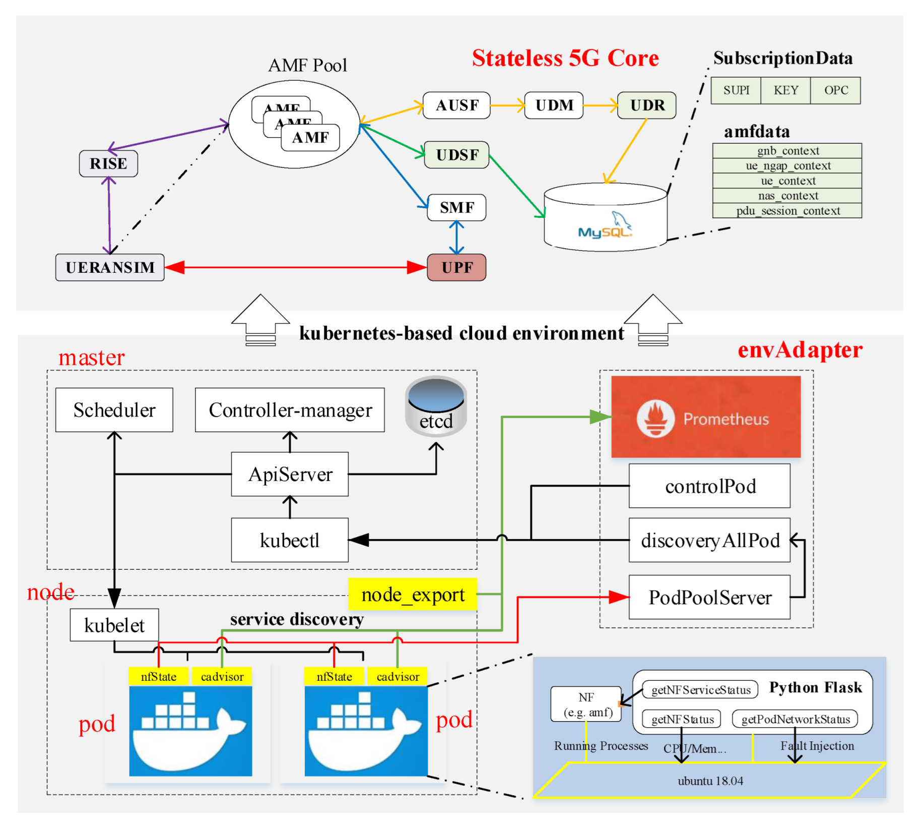As is shown in Figure 2, the stateless 5G core network consists of RAN Service Integrated Enabler (RISE), AMF, SMF, UDM, AUSF, UDR, UDSF, and UPF. RISE is a middleware between UERANSIM and AMF, responsible for the mutual conversion of HTTP1.1 and SCTP protocols to discover AMF instances. The SCTP protocol within AMF is replaced by HTTP1.1 to send/receive non-access-stratum (NAS) messages. Further, the communication contexts within AMF are removed to the unified data storage, UDSF, to make AMF stateless. When receiving one NAS message by AMF, it will try to obtain the corresponding contexts associated with someone’s identifier (e.g., SUPI) first. The processing results will also be updated in UDSF to ensure information consistency. UDSF maintains an MYSQL database storing contexts such as gnb_context, ue_ngap_context, and so on. With these network functions, the stateless 5G core network is able to inter-operate with open-source gNB/UE (e.g., UERANSIM) and also some commercial gNBs (e.g., Baicell, Amarisoft gNB) and UEs (e.g., Huawei Mate 30 5G Pro, Hongmi K30). Therefore, some high-level features such as UE-initiated registration and PDU session establishment procedures can be supported for real 3GPP-defined signaling messages. In order to collect the network-domain and service-domain data within the cloud-native 5G core network, some modifications are made to the state-of-the-art open-source projects. The “EventExposure” service within AMF and SMF is implemented to expose network-domain data, such as UEs’ SUPI, IP address UEs’ location, and so on. For UPF, we implement a non-3GPP-defined interface for UPF to expose the service-domain data such as uplink and downlink data rate of a certain UE because 3GPP has not designed the service-based interfaces for UPF.

Kubernetes-based Cloud Environment. The stateless 5G core network is implemented to be adaptable in the cloud environment with instances packaged in Docker containers. Kubernetes, an open-source cloud environment, is chosen to orchestrate all NF instances in this PoC prototype. As is shown in Figure 2, we integrate Prometheus into Kubernetes to collect the resource-domain data automatically. Prometheus is an open-source monitor for resource utilization of physical machines, virtual machines, Kubernetes nodes, and Kubernetes Pods deploying NF instances. To make this happen, each Kubernetes worker node is equipped with node_export, each Pod is equipped with cadvisor, and Prometheus should be configured to support the service discovery procedure within Kubernetes.

There exists one situation that one Pod may be alive while the NF instance deployed in this Pod may crash because of some bugs. In this context, we customize a Python service named nfState.py that will work after one Pod is instantiated. It implements three interfaces to collect network-domain and service-domain data of NFs and control the resource utilization (e.g., CPU, memory); therefore, we can check if the Python service is alive to judge if the NF instance is available. getNFStatus is used to obtain the running-time process identity (PID), CPU, memory, traffic load information, and/or static capacity of NF instances. getNFServiceStatus is used to obtain the signaling status of UE and/or running-time downlink/uplink traffic data. getPodNetworkStatus is used to obtain the delay and packet loss rate information of the NF instances.

On top of the basic environment, we implement the envAdapter to provide unified APIs for data collection and network control. Three Python services are implemented to reach this target, including controlPod, discoveryAllPod, and PodPoolServer. The controlPod service exposes the capabilities of horizontal or vertical scaling of NF instances (e.g., adding a new Pod instance). The discoveryAllPod service is used to obtain the IP addresses of all available network function instances to support network-domain service discovery procedures. The PodPoolServer service integrates network data from different domains (e.g., network-domain, resource-domain, and service-domain) together, facilitating graph-based association and then exposing them to the AIE.

3.2. The Artificial Intelligence Engine Deploying DRL Algorithms

In order to provide AI-native functionalities for the agent to learn from the collected state of the underlying networks, we consider that there will be a scalable and effective engine running multiple and customized DRL algorithms in real-world systems.

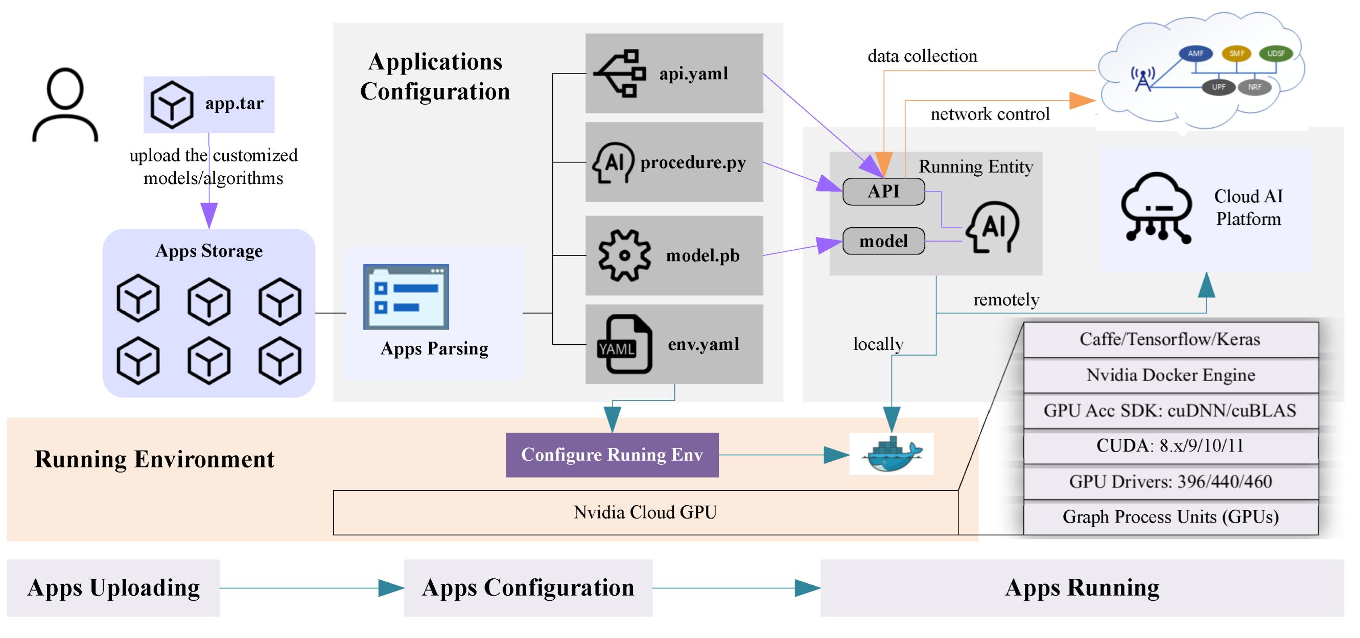
For this purpose, we develop an AIE referring to NVIDIA Cloud GPU solutions and implement a procedure for customized AI algorithms uploading, parsing, and running, which is illustrated in Figure 3. As is shown, the procedure includes “Apps Uploading”, “Apps Configuration”, and “Apps Running” in order. The model designer first uploads the application package (app.tar) that consists of the AI models/algorithms and requirements for running environment/network data. The application package will be stored in the “apps” database, waiting to be parsed and allocated with one or more NVIDIA Docker instances.

During “Apps Configuration”, the application package is decompressed with four files that are “api.yaml”, “env.yaml”, “model.pb”, and “procedure.py”, respectively. The “api.yaml” indicates the required network data for training the uploaded AI model and the network control interfaces for executing generated actions (or decisions). The AIE maintains all APIs for network data retrieval and network control and opens them all to ensure their availability for model designers. Moreover, different AI models/algorithms may be written with a different version of Python and neural networks so that the running environment requirements should be indicated specifically in “env.yaml”. For example, one AI model/algorithm may run with Python 3.6 and Tensorflow 2.0 supporting GPU, while another one may run with Python 3.5 and Pytorch. The model designer may upload a pre-trained model optionally that is in the format of “model.pb”. The main logic of the AI model/algorithm, including data retrieval, model training, model inference, and decision-making, is written in “procedure.py”. With the four files, NWDAF then assigns the AI model/algorithm with one or more compliant NVIDIA Docker instances for running.

Afterward, the AI model/algorithm running in NVIDIA Docker obtains the network data from the “data” database following the configured data APIs. The generated results can be used for network control following the configured network control APIs; therefore, the MAPE closed-loop architecture is implemented in the AIE, which facilitates the online network automation for a cloud-native 5G core network.

3.3. Implementation

The prototype runs on four virtual machines (VMs) deployed on one SANGFOR (https://www.sangfor.com.cn/ (accessed on 2 October 2022)) server, including three VMs for deploying a Kubernetes (One master and two work nodes: 8-cores CPU, 8G memory, Ubuntu 18.04; Kubernetes version: 1.17.4)-based cloud environment and one VM (AIE: 32-cores CPU; 32G memory; Ubuntu 18.04; GPU version: NVIDIA A100-PCI; NVIDIA-SMI 470.141.03; CUDA version 11.4; cuDNN version: v8.2.4; installation tutorials for NVIDIA Cloud GPU: https://zhuanlan.zhihu.com/p/406815658 (accessed on 2 October 2022)) for deploying an AIE. 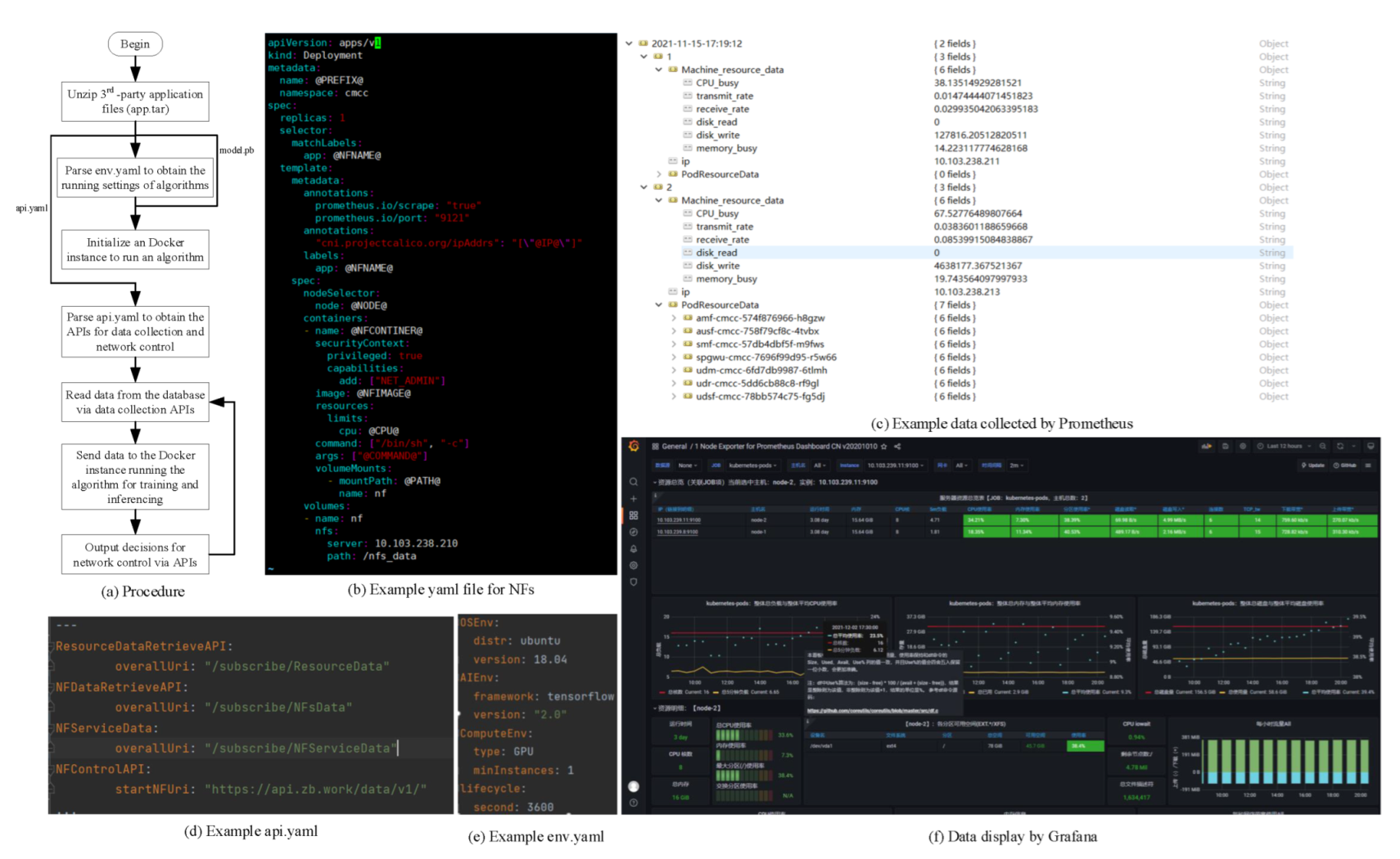The communication between Kubernetes nodes is via a Flannel plugin with which a Calico (https://www.cnblogs.com/xin1006/p/14989365.html (accessed on 2 October 2022)) plugin is integrated to maintain the IP addresses of Pods. Each NF is packaged in one Docker instance via one specific Dockerfile shown in Figure 4b to be deployed in a Pod on one work node.

• @PREFIX@: The unique name of deployment of the Docker instance, e.g., amf.
• @NFNAME@: The unique name of Pod when deploying different instances, e.g., amf.
• @IP@: The unique IP address of Pod is set supported by the Calico plugin, e.g., 10.244.1.19.
• @NODE@: The selected node to deploy a new Pod instance, e.g., node2.
• @NFCONTAINER@: The name of newly created container, e.g., amf-1.
• @NFIMAGE@: The selected image file to create a new Pod instance (the image file shall be available on the selected node), e.g., amf:cmcc.
• @CPU@: The required CPU resource, e.g., 50 m. If the available CPU resource of the selected node is lower than the required one, the Pod instance cannot be created successfully.
• @COMMAND@: The commands to run the scripts (nfState.py for opening the states of the Pod instance) and the executable file of NF (e.g., /amf/build/amf/build/amf –c /home/amf.conf -o).
• @PATH@: The file sharing path between the container and the host, e.g., /home/.

The whole procedure is illustrated in Figure 4a. Firstly, users upload their 3rd-party applications packaged in compressed files (e.g., app.tar). The AIE unzips these files to obtain four elements including “env.yaml”, “api.yaml”, “procedure.py”, and “model.pb”. An example “env.yaml” is shown in Figure 4e, which indicates the requirements of the running environment; an example “api.yaml” is shown in Figure 4d, which indicates the APIs for data collection and network control. With the “env.yaml” file, the AIE creates a new NVIDIA Docker instance to the application with “procedure.py” (logic of the algorithms) and “model.pb” (non-trained or trained neural network). The data manager within the AIE periodically collects state data from the underlying environment and provides many fine-grained APIs for data openness. The example data collected by Prometheus are shown in Figure 4c, which can also be displayed graphically via Grafana.

4. Use Case: Delayed-DQN-Enabled AMF Scaling

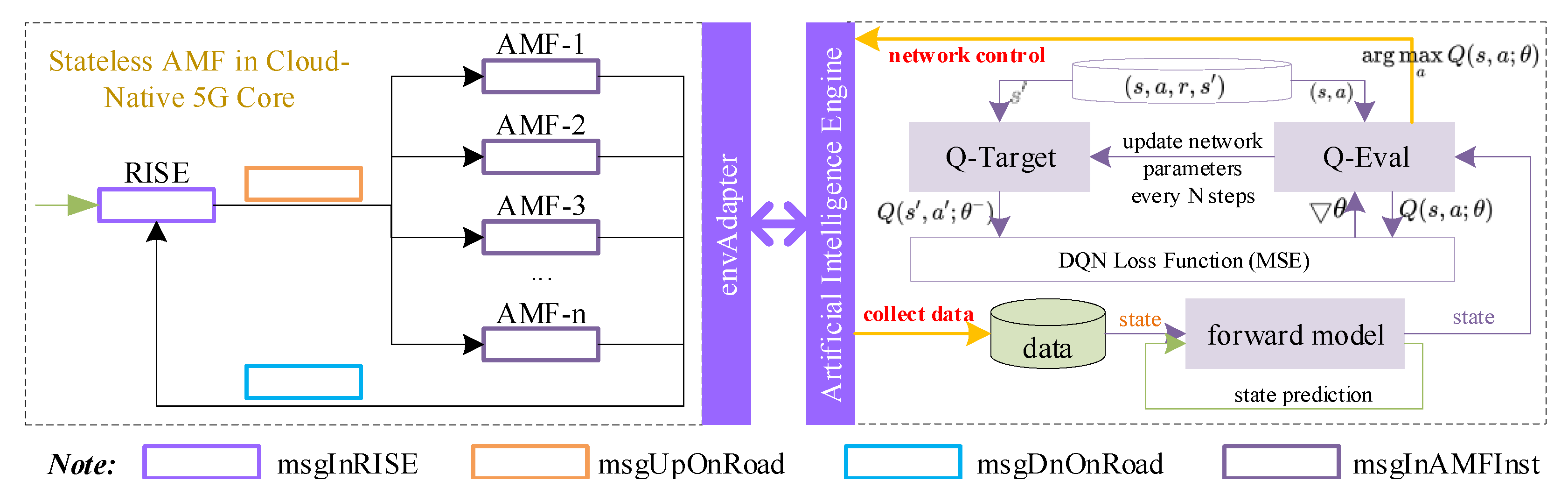
On top of the PoC prototype, we implement a use case to evaluate our proposed random-delay-corrected DRL framework. In the 5G core network, AMF is of vital importance for connecting the radio access networks and core networks, which may result in performance bottlenecks. Our previous work [21] has designed and implemented a message-level stateless AMF that helps to realize signaling-no-loss and UE-unaware scaling; therefore, we choose to implement a delayed-DQN-enabled AMF scaling use case for the validation. The architecture is illustrated in Figure 5.

Within the environment, multiple AMF instances collaborate together to process signaling messages. RISE performs as a middle box between the radio access networks and the 5G core networks, which inherit the SCTP server from AMF. RISE receives all signaling messages and mixes them without considering the procedures or UEs that individual message belongs to. Moreover, stateless AMF is implemented by decoupling the communication contexts from the functional procedures. In this context, RISE can distribute all signaling messages into multiple AMF instances to be processed, thus supporting UE-unaware message-level load balancing.

We abstract the working model as the left figure of Figure 5. Each component (e.g., RISE, AMF) is with a message queue for caching unprocessed signaling messages. For example, the purple rectangle named “msgInRISE” is the message queue within RISE to cache the upcoming signaling request messages with the Poisson distribution. Additionally, “msgUpOnRoad” and “msgDnOnRoad” represent the uplink/downlink signaling messages that are still on the road to the peer entities for simplification. The service rate of “msgInRISE” and “msgInAMFInst” is related to the processing capabilities of RISE and AMF instances, while that of “msgUpOnRoad” and “msgDnOnRoad” is related to the uplink and downlink delays between RISE and AMF instances. Moreover, the signaling messages from RISE are distributed to the AMF instance that has a minimum number of unprocessed messages one by one to be balanced among multiple AMF instances. The target is to allocate an adaptive number of stateless AMF instances to process the upcoming request messages at a low cost.

4.1. Reinforcement Learning

For this purpose, the problem is modeled as a MDP, including state representation, action definition, and reward description that are illustrated as follows:

State Representation: The state is represented as $S=(\mathbf{N},\mathbf{D},{\mathbf{C}}_{amf},{\mathbf{N}}_{amf})$. $\mathbf{N}$ is defined as the vector of a number of messages in “msgInRISE” ($N_{rise}$), “msgUpOnRoad” ($N_{up}$), and “msgDnOnRoad” ($N_{dn}$) message queues, that is $\mathbf{N}=(N_{rise},N_{up},N_{dn})$. $\mathbf{D}$ donates the vector of uplink ($D_{up}$) and downlink ($D_{dn}$) delays between RISE and AMF instances, that is $\mathbf{D}=(D_{up},D_{dn})$. ${\mathbf{C}}_{amf}$ represents the vector of the number of CPU cores of AMF instances, that is ${\mathbf{C}}_{amf}=(C_{amf-1},C_{amf-2},\dots ,C_{amf-N_{max}})$ and ${\mathbf{N}}_{amf}$ represents the vector of number of the unprocessed messages within AMF instances, that is ${\mathbf{N}}_{amf}=(N_{amf-1},N_{amf-2},\dots ,N_{amf-N_{max}})$, where $N_{max}$ is the maximum number of AMF instances supported in the system. For AMF instances that are not instantiated, the corresponding number of CPU cores and unprocessed messages is 0.

Action Definition: An action is a valid decision on the number of AMF instances, which may be “$-1$”, “0”, or “1”. “$-1$” means that envAdapter deletes one AMF instance if the number of AMF instances is more than 1. The unprocessed messages in the to-be-deleted AMF instance are equally distributed among other live AMF instances. The AMF instance can accept these messages unless the number of unprocessed messages itself does not exceed its 90% of maximum capacity ($C_{max}$) so some messages may be discarded. “0” means that the environment keeps running without any change in the number of AMF instances. “1” means that a new AMF instance will be instantiated if the number of AMF instances is less than $N_{max}$.

Reward Description: A reward is a signal telling the agent how good the current action is doing. The reinforcement learning agent aims to maximize the estimation of discounted accumulative rewards to obtain better long-term performance. In this use case, the agent is envisioned to learn an optimal policy for deploying an adaptive number of AMF instances under UE signaling requests lasting for certain time steps with a Poisson distribution. The reward function is defined as (20). Firstly, the current number of AMF instances $N_{aft}$ is calculated as (17), where $N_{cnt}$ denotes the number of AMF instance before executing an action. Then, the average capacity ($C_{avg}$) of unprocessed signaling messages among all AMF instances is calculated as (18), where $N_{total}$ denotes the total number of unprocessed signaling messages in the system, $S_{cp}$ denotes the processing capability of AMF instances (messages per second), and T denotes the running time before arriving at next time step. When $C_{avg}$ exceeds the $0.9$ times maximum capacity $C_{max}$, we set $C_{avg}=2C_{max}$ to calculate a negative reward value to punish such actions. Then, the basic reward value $R_{base}$ is calculated as (19), considering the QoS for processing signaling messages and the costs for deploying AMF instances at the same time. In order to limit the reward value in each step to $[0,1]$, the reward value is normalized as defined in (20); therefore, we obtain the final reward value $R_{final}$.

$$(N_{aft},R_{punish})=\left\{\begin{array}{ccc}\hfill (N_{cnt}+1,0)& & a=1and{N}_{cnt}<N_{max}\hfill \\ \hfill (N_{cnt},-0.5)& & a=1and{N}_{cnt}=N_{max}\hfill \\ \hfill (N_{cnt},0)& & a=0\hfill \\ \hfill (N_{cnt},-0.5)& & a=-1and{N}_{cnt}=1\hfill \\ \hfill (N_{cnt}-1,0)& & a=-1and{N}_{cnt}>1\hfill \end{array}\right.$$

(17)

$$C_{avg}=\left\{\begin{array}{ccc}\hfill N_{total}/N_{aft}-S_{cp}\times T& & C_{avg}\le 0.9C_{max}\hfill \\ \hfill 2C_{max}& & C_{avg}>0.9C_{max}\hfill \end{array}\right.$$

(18)

$$R_{base}=\alpha (0.9-C_{avg}/C_{max})/0.9-N_{aft}/N_{max}+R_{punish}$$

(19)

$$R_{final}=(R_{base}-(-3.3))/(1-N_{aft}/N_{max}-(-3.3))$$

(20)

4.2. Experiment Setup and Parameters

In this experiment, three types of signaling requests including RegistrationRequest, ServiceRequest, and PDUSessionEstablishmentRequest were simulated by UERANSIM following the $sin(·)$-like flow pattern (that is $500sin(x)+500$). There are flows varying from $[0,1000]$ in 10 time steps. Each type of signaling request is processed via a service function chain (e.g., RegistrationRequest is processed via a 〈AMF-AUSF-UDM-UDR〉 chain). Further, each type of signaling request has different resource (e.g., CPU) requirements in different network functions and has different ttl. The detailed parameters for signaling requests are shown in

Table 1. Parameters for signaling requests.

Signaling Request	Chain	CPU Requirements (Cycles/s)	ttl (Time Steps)
RegistrationRequest	〈 AMF-AUSF-UDM-UDR 〉	$\langle 100,200,400,500\rangle$	3000
ServiceRequest	〈 AMF-AUSF-UDM-UDR 〉	$\langle 200,300,100,400\rangle$	2800
PDUSessionEstablishmentRequest	〈 AMF-SMF-UDM-UPF 〉	$\langle 315,246,177,63\rangle$	4000

.

In addition, we deploy four instances for each network function except AMF and maximum $N_{max}=30$ AMF instances in this use case to process these signaling requests. In the beginning, there is only one AMF instance available and the agent will decide to add/delete/maintain the number of AMF instances according to the received state time by time. For each instance, the maximum capacity and CPU are set to be $C_{max}=5000$ and $300 \mathrm{cycles}/\mathrm{s}$. Neural networks’ parameters are shown in

Table 2. Parameters for neural networks.

Neural Networks	Architecture	Learning Rate	Training Index	Updating Index	Batch Size
Evaluation/Target Q	128 (relu) - 64 (relu) - 3 (linear)	$0.0001$	10	20	32
Forward Model	128 (relu) - 64 (relu) - 8 (sigmod)	$0.0001$	10	$None$	32

.

The experiment will run for $EPISODE=500$ episodes and 20,000 time steps for each one. In order to explore the possible states in the environment, we set the maximum epsilon and epsilon decay to be ${ϵ}_{max}=0.9$ and ${ϵ}_{decay}=0.99996$, respectively. At each time step, the agent will randomly choose an action with a probability $ϵ$ and then $ϵ$ will be changed to be $ϵ=ϵ\times {ϵ}_{decay}$ until it reaches ${ϵ}_{max}$.

4.3. Benchmark Scenarios

To evaluate the performance and feasibility of our proposed random-delay-corrected DRL framework (delayed-DQN in this use case), we design the following scenarios:

• No-delay scenario. This is an idle scenario with the assumption that the collected state will arrive at the agent immediately without delays; therefore, delayed-DQN works the same as the standard DQN.
• Turn-based scenario. There are constant or random delays between the agent and the environment, but the agent will only generate an action when it receives the collected state, whose interaction pattern is shown in Figure 1a.
• Constant-delay scenario with the standard DQN. In this scenario, the delays are transformed to be constant delays by carefully choosing the time interval $\mathsf{\Delta }T$ as presented in Section 2.3. Then, the interaction pattern works as shown in Figure 1b. The standard DQN (DQN algorithm with the standard MDP) is used to try to learn an optimal policy for better AMF scaling.
• Random-delay scenario with the standard DQN. We design a scenario where the standard DQN tries to learn an optimal policy in a random-delay environment.
• Constant-delay scenario with delayed-DQN. Different from the above scenario, this scenario adopts our proposed delayed-DQN to learn an optimal policy.
• Random-delay scenario with delayed-DQN. This agent is equipped with the delayed-DQN algorithm to learn from delay-corrected trajectories sampling in a random-delay scenario.

4.4. Evaluation Results

The evaluation results are shown in Figure 6. As we can see from Figure 6a, the no-delay scenario shows the optimal training results compared to others while the turn-based scenario shows the worst performance, which proves that the turn-based pattern cannot adapt to the dynamics in the real-world networks. However, we can still figure out that the periodicity-based pattern shown in Figure 1b,c cannot train an optimal agent when the standard DQN algorithms are used, especially for the random-delay scenario. Although the constant-delay scenario with the standard DQN trains a near-optimal agent, the reward has high fluctuation that can affect the final decisions. Moreover, the random-delay scenario with the standard DQN even has little improvement compared to the turn-based scenario. The results tell us we can not adopt the standard DQN algorithm to the periodicity-based scenarios directly, which cannot guarantee performance. After that, our proposed delayed-DQN based on the random-delay-corrected DRL framework is integrated with the periodicity-based pattern for the validation. The results show that the performance of the delayed-DQN algorithm is very close to the optimal value of the no-delay scenario for both constant-delay and random-delay scenarios. Figure 6b–f evaluate the impact of the state collection time interval $\mathsf{\Delta }T$ on the performance of DQN algorithms. For the evaluation, we set three different $\mathsf{\Delta }T$ values, which are 20, 10, and 5 time steps, respectively. Generally, we can see that it performs better when for $\mathsf{\Delta }T=5$ than the other two scenarios no matter what interaction pattern is chosen. The results prove that frequent state collection with smaller time intervals $\mathsf{\Delta }T$ can better adapt to network dynamics.

In summary, Figure 6 proves that (1) the periodicity-based pattern can be more beneficial to capture the network dynamics than the turn-based pattern; (2) the random-delay-corrected DRL framework can improve the performance when adopting the DQN algorithm in the periodicity-based scenarios; (3) smaller state collection time interval $\mathsf{\Delta }T$ can further improve the performance of the delayed-DQN algorithm.

5. Conclusions

This paper proposes a random-delay-corrected deep reinforcement learning framework to address the challenges for DRL algorithms application in real-world networks where random delays exist between the agent and the environment. Firstly, the interaction patterns are abstracted to be three scenarios including turn-based, periodicity-based with constant delays, and periodicity-based with random-delays scenarios. Secondly, these interaction patterns are modeled as a partial history-dependent Markov decision process, which extends from the standard Markov decision process. Thirdly, a random-delay-corrected deep reinforcement learning framework with a forward model and delay-corrected trajectory sampling is presented to transform the PH-MDP to the standard MDP, thereby training the agent using the state-of-the-art DRL algorithms. Fourthly, an example DRL algorithm, namely delayed-DQN, based on the framework is proposed. For the evaluation, a PoC prototype for a cloud-native 5G core network is developed and a use case, namely delayed-DQN-enabled AMF (one network function in 5G core network) scaling, is implemented. The evaluation results show that the proposed methodologies perform better in the random-delay networks than others. This paper makes good contributions to DRL-enabled online closed-loop management for real-world networks thereby enabling AI-native network automation towards 6G.

References

1. Khan, L.U.; Saad, W.; Niyato, D.; Han, Z.; Hong, C.S. Digital-Twin-Enabled 6G: Vision, Architectural Trends, and Future Directions. IEEE Commun. Mag. 2022, 60, 74–80. [Google Scholar] [CrossRef]
2. Taleb, T.; Aguiar, R.L.; Grida Ben Yahia, I.; Chatras, B.; Christensen, G.; Chunduri, U.; Clemm, A.; Costa, X.; Dong, L.; Elmirghani, J.; et al. White Paper on 6G Networking. 2020. Available online: https://biblio.ugent.be/publication/8668820 (accessed on 30 October 2022).
3. Li, N.; Liu, G.; Zhang, H.; Zhao, Q.; Zhao, Y.; Tong, Z.; Wang, Y.; Sun, J. Micro-service-based radio access network. China Commun. 2022, 19, 1–15. [Google Scholar] [CrossRef]
4. Zeydan, E.; Mangues-Bafalluy, J.; Baranda, J.; Requena, M.; Turk, Y. Service Based Virtual RAN Architecture for Next Generation Cellular Systems. IEEE Access 2022, 10, 9455–9470. [Google Scholar] [CrossRef]
5. Liu, G.; Huang, Y.; Li, N.; Dong, J.; Jin, J.; Wang, Q.; Li, N. Vision, requirements and network architecture of 6G mobile network beyond 2030. China Commun. 2020, 17, 92–104. [Google Scholar] [CrossRef]
6. Shen, X.; Gao, J.; Wu, W.; Li, M.; Zhou, C.; Zhuang, W. Holistic Network Virtualization and Pervasive Network Intelligence for 6G. IEEE Commun. Surv. Tutorials 2021, 24, 1–30. [Google Scholar] [CrossRef]
7. Samdanis, K.; Taleb, T. The road beyond 5G: A vision and insight of the key technologies. IEEE Netw. 2020, 34, 135–141. [Google Scholar] [CrossRef]
8. Wu, J.; Li, R.; An, X.; Peng, C.; Liu, Z.; Crowcroft, J.; Zhang, H. Toward native artificial intelligence in 6G networks: System design, architectures, and paradigms. arXiv 2021, arXiv:2103.02823. [Google Scholar]
9. Yao, J.; Chen, M. A Flexible Deployment Scheme for Virtual Network Function Based on Reinforcement Learning. In Proceedings of the 2020 IEEE 6th International Conference on Computer and Communications (ICCC), Chengdu, China, 11–14 December 2020; pp. 1505–1510. [Google Scholar] [CrossRef]
10. Jin, H.; Pang, W.; Zhao, C. AMF Optimal Placement based on Deep Reinforcement Learning in Heterogeneous Radio Access Network. 2020. Available online: https://www.researchsquare.com/article/rs-14323/v1 (accessed on 2 October 2022).
11. Nguyen, H.T.; Do, T.V.; Hegyi, A.; Rotter, C. An Approach to Apply Reinforcement Learning for a VNF Scaling Problem. In Proceedings of the 2019 22nd Conference on Innovation in Clouds, Internet and Networks and Workshops (ICIN), Paris, France, 19–21 February 2019; pp. 94–99. [Google Scholar] [CrossRef]
12. Yan, Z.; Ge, J.; Wu, Y.; Li, L.; Li, T. Automatic Virtual Network Embedding: A Deep Reinforcement Learning Approach With Graph Convolutional Networks. IEEE J. Sel. Areas Commun. 2020, 38, 1040–1057. [Google Scholar] [CrossRef]
13. Sun, P.; Lan, J.; Li, J.; Guo, Z.; Hu, Y. Combining Deep Reinforcement Learning With Graph Neural Networks for Optimal VNF Placement. IEEE Commun. Lett. 2021, 25, 176–180. [Google Scholar] [CrossRef]
14. Kim, J.; Lee, J.; Kim, T.; Pack, S. Deep Reinforcement Learning based Cloud-native Network Function Placement in Private 5G Networks. In Proceedings of the 2020 IEEE Globecom Workshops GC Wkshps, Taipei, Taiwan, 7–11 December 2020; pp. 1–6. [Google Scholar] [CrossRef]
15. Li, J.; Shi, W.; Zhang, N.; Shen, X. Delay-Aware VNF Scheduling: A Reinforcement Learning Approach With Variable Action Set. IEEE Trans. Cogn. Commun. Netw. 2021, 7, 304–318. [Google Scholar] [CrossRef]
16. Ramstedt, S.; Pal, C. Real-time reinforcement learning. In Advances in Neural Information Processing Systems 32; 2019; Available online: https://proceedings.neurips.cc/paper/2019/hash/54e36c5ff5f6a1802925ca009f3ebb68-Abstract.html (accessed on 30 October 2022).
17. Travnik, J.B.; Mathewson, K.W.; Sutton, R.S.; Pilarski, P.M. Reactive Reinforcement Learning in Asynchronous Environments. Front. Robot. AI 2018, 5, 79. [Google Scholar] [CrossRef] [PubMed] [Green Version]
18. Chen, B.; Xu, M.; Li, L.; Zhao, D. Delay-aware model-based reinforcement learning for continuous control. Neurocomputing 2021, 450, 119–128. [Google Scholar] [CrossRef]
19. Ramstedt, S.; Bouteiller, Y.; Beltrame, G.; Pal, C.; Binas, J. Reinforcement Learning with Random Delays. arXiv 2020, arXiv:2010.02966. [Google Scholar]
20. Vittal, S.; Franklin A., A. Self Optimizing Network Slicing in 5G for Slice Isolation and High Availability. In Proceedings of the 2021 17th International Conference on Network and Service Management (CNSM), Izmir, Turkey, 25–29 October 2021; pp. 125–131. [Google Scholar]
21. Du, K.; Wang, L.; Wen, X.; Liu, Y.; Niu, H.; Huang, S. ML-SLD: A message-level stateless design for cloud-native 5G core network. Digit. Commun. Net. 2022. [Google Scholar] [CrossRef]
Figure 1. Different interaction scenarios between the agent and the underlying networks considering different delay patterns. d 1 and d 2 are delays for state collection and action execution, respectively. T denotes the time interval of state collection and T is the time interval of action execution. The red symbols such as “x” (as shown in (c)) mean that the collected states will not be used to generate the next action. The red lines are the processes for state collection, while the green lines are for action execution. Here, we assume that the action delays are constant.
Applsci 12 12297 g001
Figure 2. Kubernetes-based cloud environment.
Applsci 12 12297 g002
Figure 3. The procedure for uploading and running customized AI models/algorithms.
Applsci 12 12297 g003
Figure 4. Procedure, example configuration file, and example data.
Applsci 12 12297 g004
Figure 5. Architecture: Delayed-DQN-enabled AMF scaling.
Applsci 12 12297 g005
Figure 6. Evaluation results. “TN”, “ND”, “CD”, and “RD” mean turn-based, no-delay, constant-delay, and random-delay scenarios, respectively. “20-TS”, “10-TS”, and “5-TS” mean Δ T is set to 20, 10, and 5, respectively. For example, “CD-DQN-5-TS” means a constant-delay scenario where states are collected every 5 time step and the agent adopts the DQN algorithm to make decisions. The results are the average rewards for each 10 episodes.
Applsci 12 12297 g006