
Study on Seismic Attenuation Based on Wave-Induced Pore Fluid Dissolution and Its Application

School of Earth Sciences, Northeast Petroleum University, Daqing 163318, China
*
Author to whom correspondence should be addressed.
Appl. Sci. 2023, 13(1), 74; https://0-doi-org.brum.beds.ac.uk/10.3390/app13010074
Submission received: 30 November 2022
/
Revised: 7 December 2022
/
Accepted: 17 December 2022
/
Published: 21 December 2022
(This article belongs to the Special Issue Technological Advances in Seismic Data Processing and Imaging)
Abstract
:Seismic wave attenuation is affected by wave-induced pore fluid dissolution. The mechanism of wave-induced pore fluid dissolution is the mutual dissolution between different fluids caused by pore fluid pressure. Compared with the traditional WIFF (wave-induced fluid flow) mechanism, the wave-induced pore fluid dissolution mechanism can predict the attenuation of the seismic frequency band and can be used in well-to-seismic calibration. Conventional methods neglect the velocity dispersion caused by the interaction between pore fluids, which will lead to errors in attenuation prediction. In this paper, we focus on accurately predicting the velocity dispersion at low porosity and permeability, which can be used in multi-scale data matching. The stretch between the synthetic data by using logging data and seismic data needs to be calibrated for more accurate interpretation. The kernel of well-to-seismic calibration is the knowledge of the velocity dispersion between the logging frequency band and seismic frequency band. We calibrate the difference between the two kinds of data by using the rock physical model. Both the model test and field data application prove the feasibility and accuracy of the proposed strategy.
1. Introduction
Wave-induced fluid flow (WIFF) is considered to be the main cause of seismic wave dispersion and attenuation in fluid-saturated porous media [1,2]. Among many theories, mesoscopic heterogeneity and microscopic heterogeneity are considered to be the main mechanisms leading to WIFF. In addition, in most rocks, the coexistence of mesoscopic heterogeneity and microscopic heterogeneity can cause a significant shift in fast p-wave velocity, which means that the effects of both mechanisms on dispersion and attenuation need to be considered simultaneously. The Squirt microscopic model mainly uses the squirt mechanism of solid/fluid interaction to estimate velocity dispersion and attenuation in fully saturated rocks [3]. Pride et al. proposed the two-pore theory to explain the corresponding seismic waves in water-bearing and gas-saturated porous media, which can explain the attenuation of magnitude 10−2 – 10−1 within the seismic frequency band. White’s model describes the complex moduli of a partially saturated spherical gas encapsulated medium and a layered medium composed of two heterogeneous porous media [4,5]. Johnson generalized gas patches of arbitrary shape [6]. In recent years, under the condition of saturated fluid and bubble phase in rock, it is believed that an obvious attenuation phenomenon will occur at the low-frequency end of an earthquake, resulting in the corresponding mechanism of gas dissolution and dissolution induced by seismic wave (pore fluid dissolution). The dissolution of wave-induced gas exsolution–dissolution is used to explain the obvious attenuation phenomenon of seismic waves [7,8,9], and these models reflect the meso-loss mechanism. Chapman measured the attenuation of two Berea sandstone samples, and the results show that compared with the WIFF mechanism, the pore fluid dissolution mechanism can be closer to the measured attenuation data [10]. Moreover, as a seismic wave attenuation mechanism, pore fluid dissolution can describe micron pores. It is more suitable for shale reservoirs with low porosity and low permeability.
Well logging data and seismic data are the two most basic forms of raw data in the process of oilfield exploration and development, and they play an important role in detailed reservoir description, including reservoir prediction. The reflected reservoir information is inconsistent, resulting in multiple solutions for reservoir prediction and description. Determining how to perform well-to-seismic matching has become an indispensable and important part of predicting reservoir lithology, physical parameters and oil potential in oil and gas exploration and development research. There are three main methods for velocity matching and calibration of well-to-seismic data:
- The Backus effective average method uses effective medium theory and a layered method to achieve high-frequency to low-frequency velocity correction. [11] deeply discussed the effect of Backus effective averaging on elastic scattering characteristics in the medium; ref. [12] used Backus effective averaging to conduct in-depth research on logging data scaling upscaling. The P and S wave velocities lead to rock physical analysis conclusions comparable to seismic scales.
- The multi-resolution analysis method stretches the signals between adjacent events of the sonic logging synthetic seismic traces to align them with the corresponding events on the side-well traces. Ref. [13] applied multi-resolution analysis technology to the resampling of logging data and the matching of synthetic records and seismic traces, and the matching accuracy was high.
- The rock physical model calibration method combines velocity dispersion theory and an absorption attenuation mechanism to achieve velocity calibration at different scales. Based on the resonant Q model [14], many researchers [15] measured the sonic logging velocity in different target blocks. Dispersion calibration was performed to improve the well–seismic matching effect. Ref. [16] combined the DEM model and the microscopic dispersion theoretical model to extrapolate the logging frequency band velocity to the seismic frequency band for well–seismic matching and inversion calculations and achieved good results in carbonate reservoirs.
In practical application, the Backus effective averaging method is simple and effective but does not consider the attenuation effect. Multiresolution analysis is highly automated but still requires accurate synthetic seismic record and stratigraphic correlation. The rock physical model calibration method can directly match data of different scales. In order to combine well logging and seismic data, it is necessary to select an appropriate rock physical model for dispersion calibration, thereby improving the accuracy of well–seismic matching.
Because the parameters of a rock physical model are large, difficult to obtain and have no actual physical significance, it is better to use a viscoelastic model instead of a rock physical model. The Zener model can fit the mesoscale White model [17], the Biot–Rayleigh model [18] and the dispersion and attenuation at two scales (meso and micro) [19]. Some researchers feel that the Cole–Cole model can more accurately simulate the acoustic properties of porous media than the rough approximation of Zener’s mechanical model [20,21], but there are five parameters, which is relatively more, while the Power Law model only needs two parameters [22], which makes it easier to use. Ref. [10] studied the seismic attenuation in Berea sandstone saturated with bidirectional fluid, compared the attenuation curves of the WIFF model and the pore fluid dissolution model under different saturation and pressure, and used SLS model to fit, and they found that the fitting effect with pore fluid dissolution is very good. Some scholars also compared multiple viscoelastic models. Paul compared the attenuation and frequency relationship curves of Maxwell Model, Voight Solid, Standard Linear, Burgers Solid and Power Law. It was found that attenuation and elastic stiffness curves vary considerably with frequency, and each model has a different variation law [23]. Toverud et al. compared eight models using the zero-offset vertical seismic profile (VSP) dataset: the Kolsky–Futterman model, Power Law model, Kjartansson model, Muller model, Azimi second model, Azimi third model, Cole–Cole model and standard linear-solid-state model (SLS). It was found that in the same depth region, the SLS model has the best results in simulating attenuation [24].
2. Materials and Methods
Rock Physics Model Upscaling by Visco-Elastic Model
Pore fluid dissolution, as an attenuation mechanism of seismic waves, will lead to dissolution and dissolution between gas and its surrounding liquid, which will lead to the attenuation of seismic waves. In the sphere area of each bubble, the gas dissolution rate can be expressed as [7]:
where dn/dt is the dissolution rate of gas, r is the bubble radius, Dw is the diffusion coefficient, Cw is the concentration, Pf is the pressure in the fluid, γ is the surface tension coefficient, R is the gas constant, T is the temperature, and KH is the Henry’s Law constant.
Rock physics models provide velocity dispersion between the seismic data and logging data for specific rock properties. Attenuation curve Qrock(f) can be used for generating synthetic seismic records:
Considering the explicit Q(f) expression in rock physics model are unavailable, visco-elastic models are upscaled with non-physical meaning parameters. Attenuation properties can then be well modeled by solving the following problem by using least-squares objective function [25,26]:
SLS model can model most rock physics models [10], and the QSLS(f) can be expressed by:
where is stress relaxation time, and τ is strain relaxation time. Combining Equations (2) and (3), the upscaled Q(f) by the SLS model can be derived:
where L is relaxation mechanisms, and is the numerically modeled attenuation curve based on the rock physics model. Here, we use the wave-induced gas exsolution–dissolution (WIGED) model to calculate the , and the parameters used are listed in Table 1. The volumetric strain of the pore fluid is calculated, followed by the modulus K, and attenuation can be obtained by
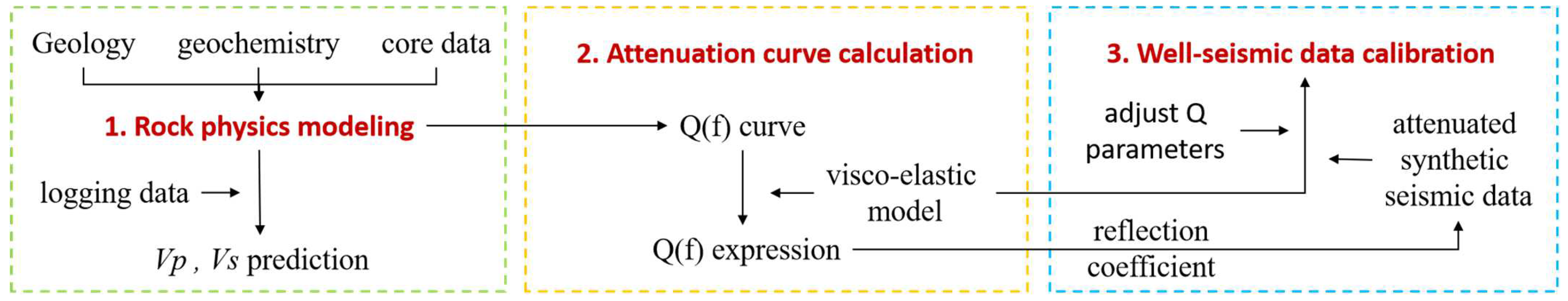
Well-to-seismic calibration based on rock physics model upscaling.
The misfit between the seismic data and the logging data can then be calibrated by implementing the following procedures (Figure 1):
- Rock physics modeling. Based on the geology, geochemistry and core data, a suitable rock physics model is selected, and the parameters in the model are upgraded. The WIGED model is used here for fluid, and the SCA model is used for rock matrix. Then, the saturated rock is obtained by Gassmann substitution. The key parameters in the WIGED model are the size of the bubble and diffusion length.
- Attenuation curve calculation. Q(f) curve is then calculated from the rock physics model. The explicit Q(f) expression can be derived through upscaling by visco-elastic model. Here, we use the SLS model for upscaling, which yields best results compared with other visco-elastic models, such as the power-law model.
- Well-to-seismic data calibration. Based on the reflection coefficient and Q(f), the attenuated synthetic seismic data can be generated. By adjusting the Q related parameters in visco-elastic model (strain relaxation time and stress relaxation time in the SLS model), the optimal match between synthetic seismic data and field data can be found.
3. Synthetic Data Test
3.1. Rock Physics Modeling and Velocity Dispersion Analyzing
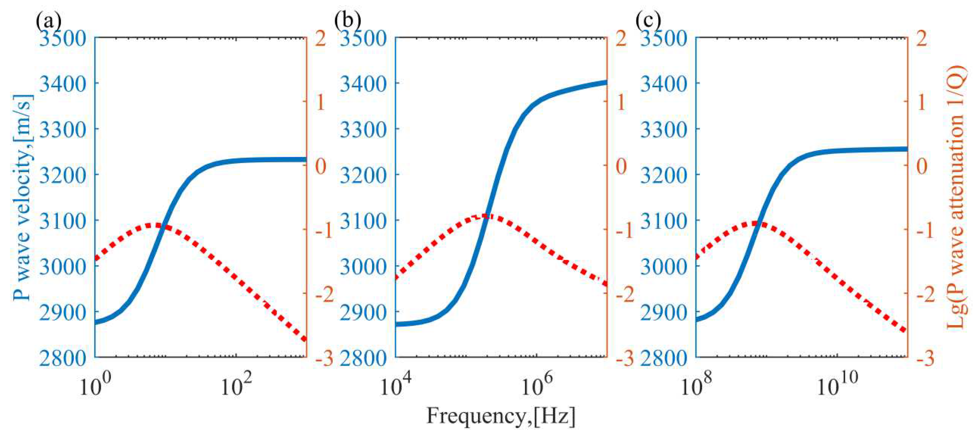
Here, three rock physics models, the pore fluid dissolution model, the SLS model and the Pride model, are applied for P-wave velocity dispersion calculation, as shown in Figure 2. Here, we consider rocks with micrometric pores, and gas micro-bubbles exist in the pores with bubble radium 1 um. Other parameters used in the models are listed in Table 1.
The corner frequency of the Squirt model is around 105 Hz, and the Pride model’s around 109 Hz. Compared with the other two models, the pore fluid dissolution model is suitable for description of this rock’s seismic frequency band, the corner frequency of which occurs between 0.1 and 100 Hz. The maximum values of the attenuation curves of the three models are similar. The Squirt model and the Pride model predict slightly larger attenuation. For the velocity dispersion, the pore fluid dissolution model and the Pride model share similar velocity range, with lower bound 2880 m/s and upper bound 3230 m/s. Although the lower bound is similar, the Squirt model yields a larger upper bound of 3400 m/s. The blue solid line is the P_wave velocity, and the red dash line is attenuation. In our model, the mobility of fluid is low due to the low porosity and low permeability, which makes it impossible for the conventional WIFF model to be used. The choice of a suitable rock physics model need to be tested by comparing the attenuation and velocity dispersion curves, and the best one is that which can model the attenuation in the seismic frequency range.
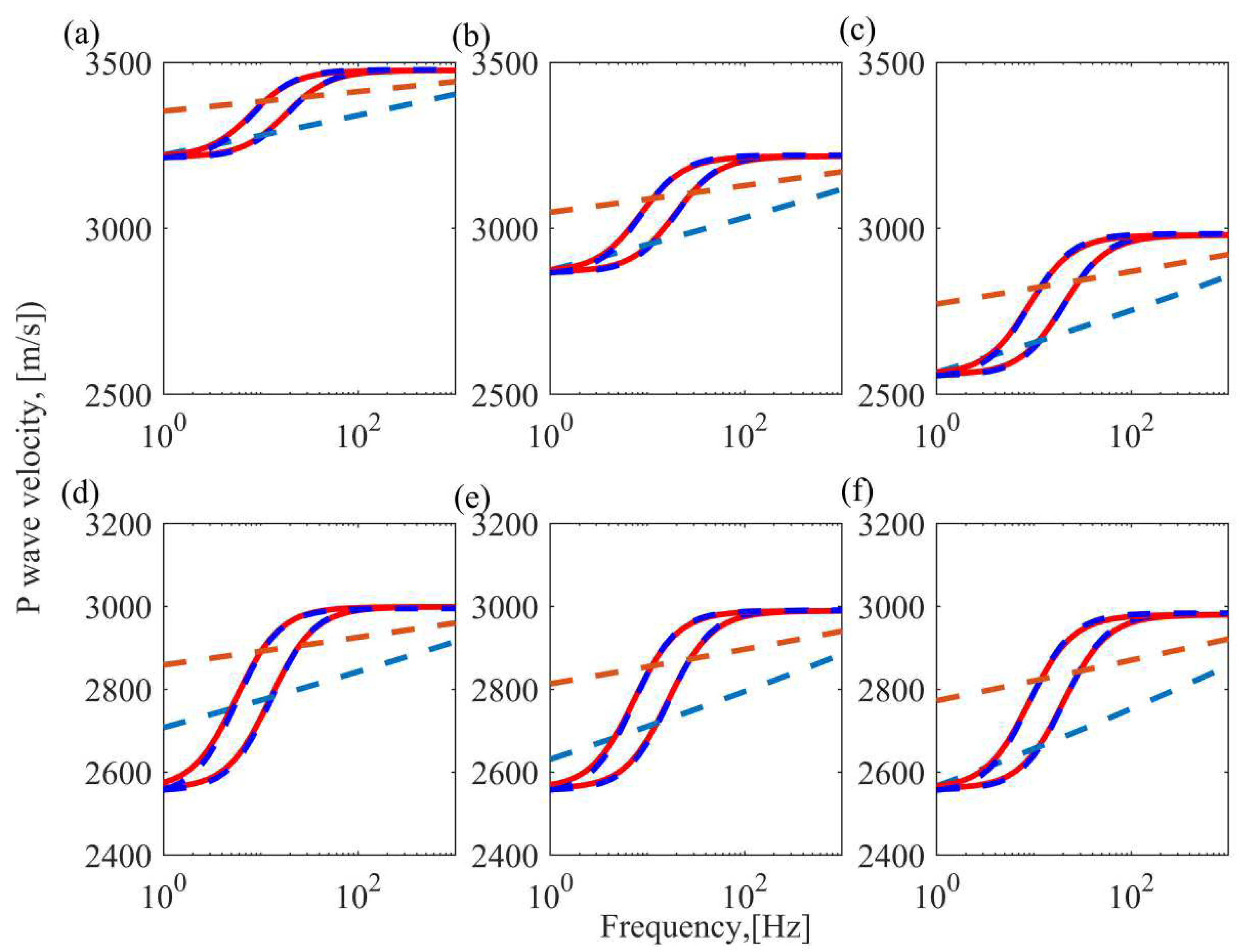
Considering that the constant Q assumption is always accepted for real data application, conventional constant Q theory is then compared for showing the velocity dispersion between logging frequency and seismic frequency. The results of velocity dispersion are shown in Figure 3. The porosity ranges from 0.04 to 0.08, and gas saturation ranges from 0.15% to 0.25%. The SLS model yields almost the same results as the pore fluid dissolution model, while the constant Q model yields a monotonous velocity curve, which contains large difference from that of the pore fluid dissolution model. As shown in Figure 3a–c, as the porosity increases, the velocity range decreases in the pore fluid dissolution model. The upper bound decreases from 3500 m/s to 3000 m/s, and the lower bound decreases from 3300 m/s to 2550 m/s. As shown in Figure 3d–f, as the gas saturation increases, the velocity range shows little difference.
The two red solid curves are the results from the pore fluid dissolution model, where the bubble radius are 4 × 10⁻⁶ and 6 × 10⁻⁶, respectively. The dash blue curves are from the SLS model. The other dash curves (orange curve and cyan curve) are from the constant Q model, and the Q values are picked from the pore fluid dissolution model at 100 Hz.
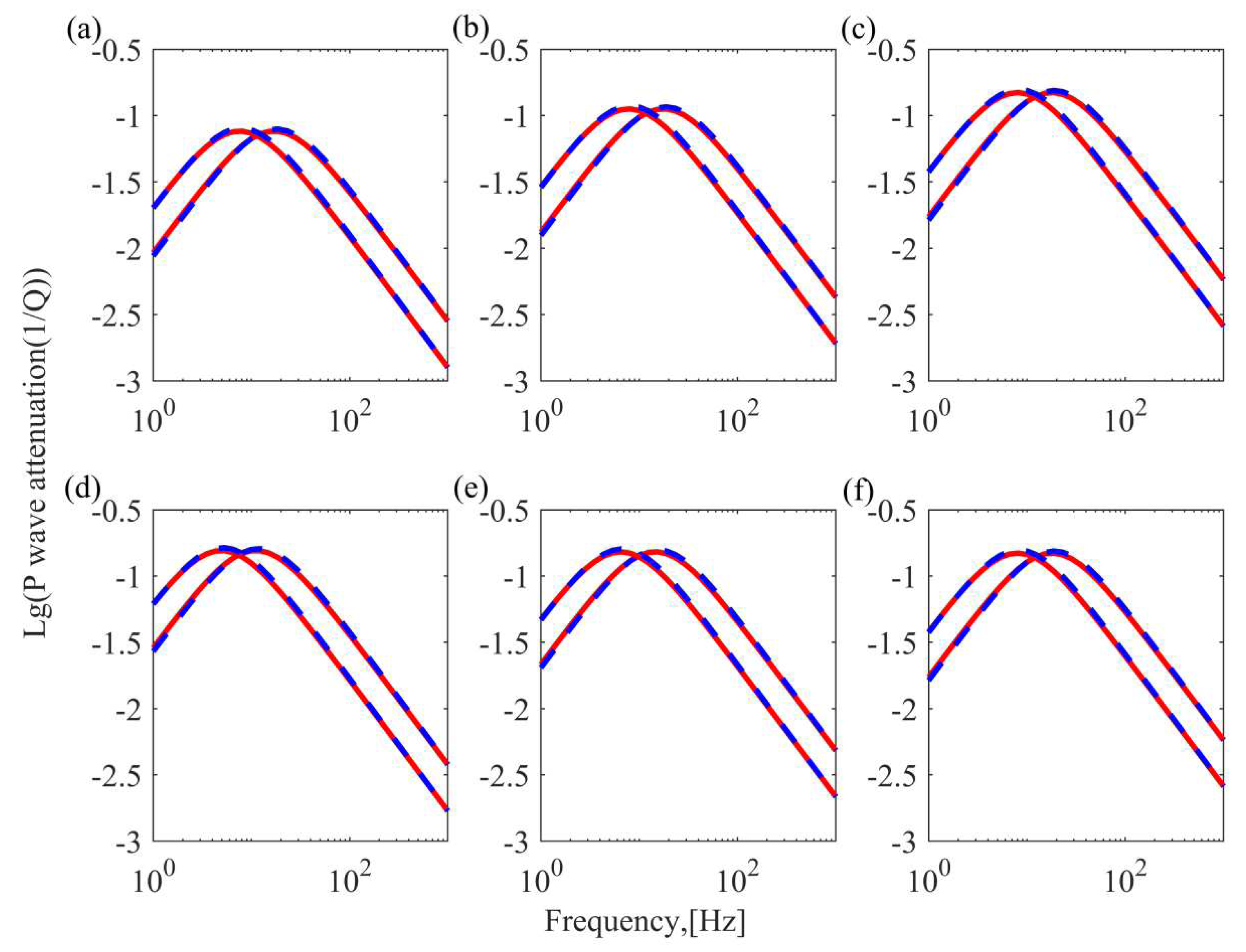
The corresponding 1/Q curves are compared in Figure 4. The two curves in each subfigure represent different bubble radii. As porosity increases, the attenuation becomes larger, while the gas saturation increase influences little about the attenuation.
3.2. Velocity Variation from Logging Data to Seismic Data Based on Rock Physics Model and Backus Averaging Method
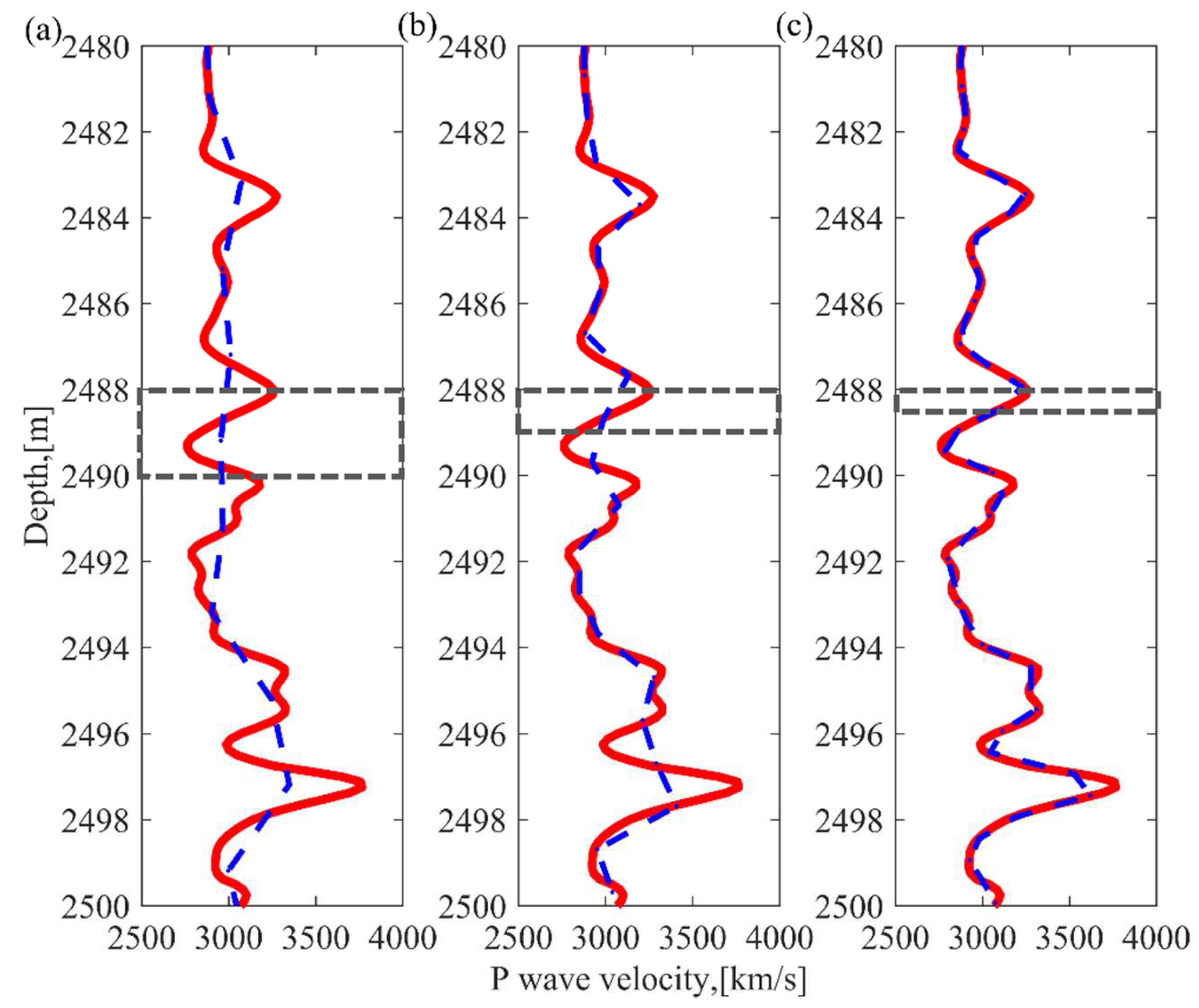
In this section, logging data is used for demonstration of velocity difference between upscaling by the pore fluid dissolution model and the Backus averaging method. Firstly, the Backus averaging method is applied, and the velocity variation is shown in Figure 5. Using different sizes of windows, the velocity results from the Backus averaging method show different properties. As the size of the window becomes larger, the velocity curve shows larger divergence from the real data. However, the velocity from all these three cases varies in the same range as that of the real data.
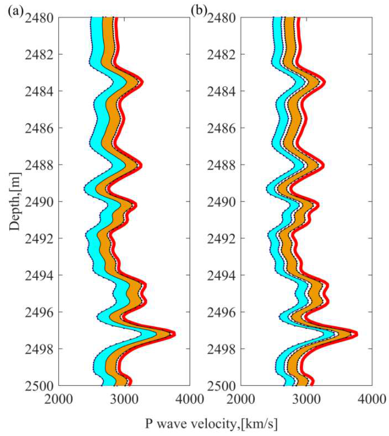
Then, the SLS model and the constant Q model are both applied to the real data for velocity correction. The results are shown in Figure 6. Compared with that of the Backus averaging method, the velocity upscaled by the SLS model and constant Q model contains obvious variation from read data. Both the models result in smaller velocity values than the real data. The SLS model always yields smaller velocity than the constant Q model in these cases.
3.3. Velocity Dispersion Correction on Synthetic Seismic Data
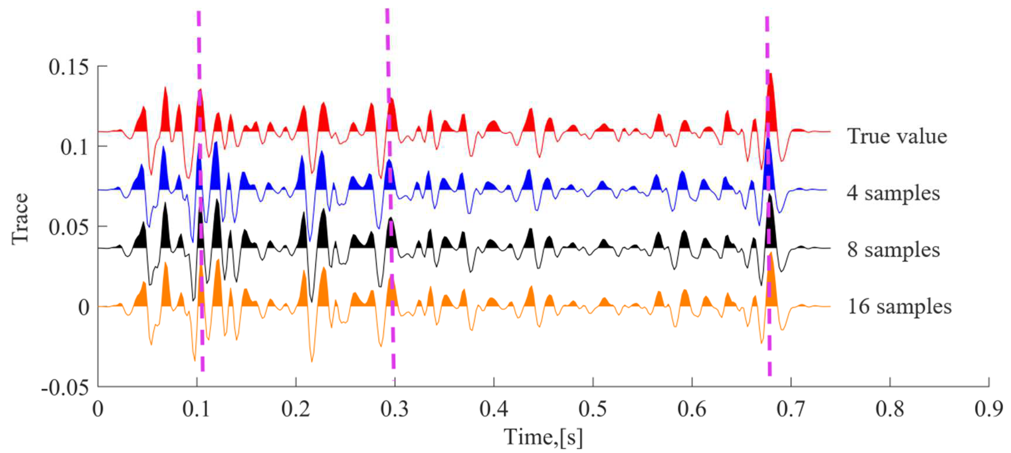
The upscaled velocities from the SLS model, the constant Q model and the Backus averaging method are all applied to the synthetic seismic data for velocity dispersion correction. The synthetic seismic data are generated by convolution of the reflection coefficient with the minimum phase wavelet. The original velocity used is that in the logging band. The amplitude of the data is not changed, as different velocity is used, only the phase. Firstly, the Backus averaging method is applied as shown in Figure 7. For windows with three different sizes, the synthetic data show little variation from the real data. The event at around 0.7 s arrives earlier that of the real data.
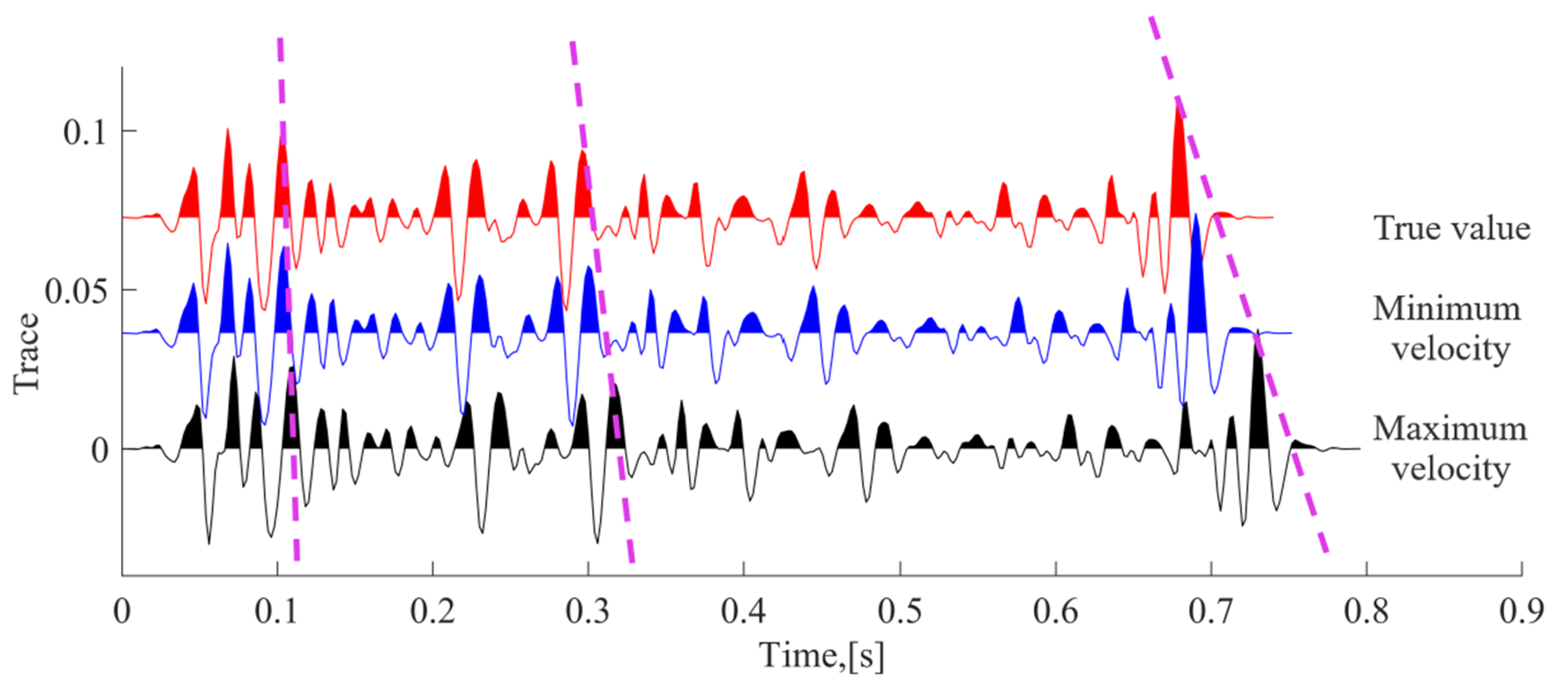
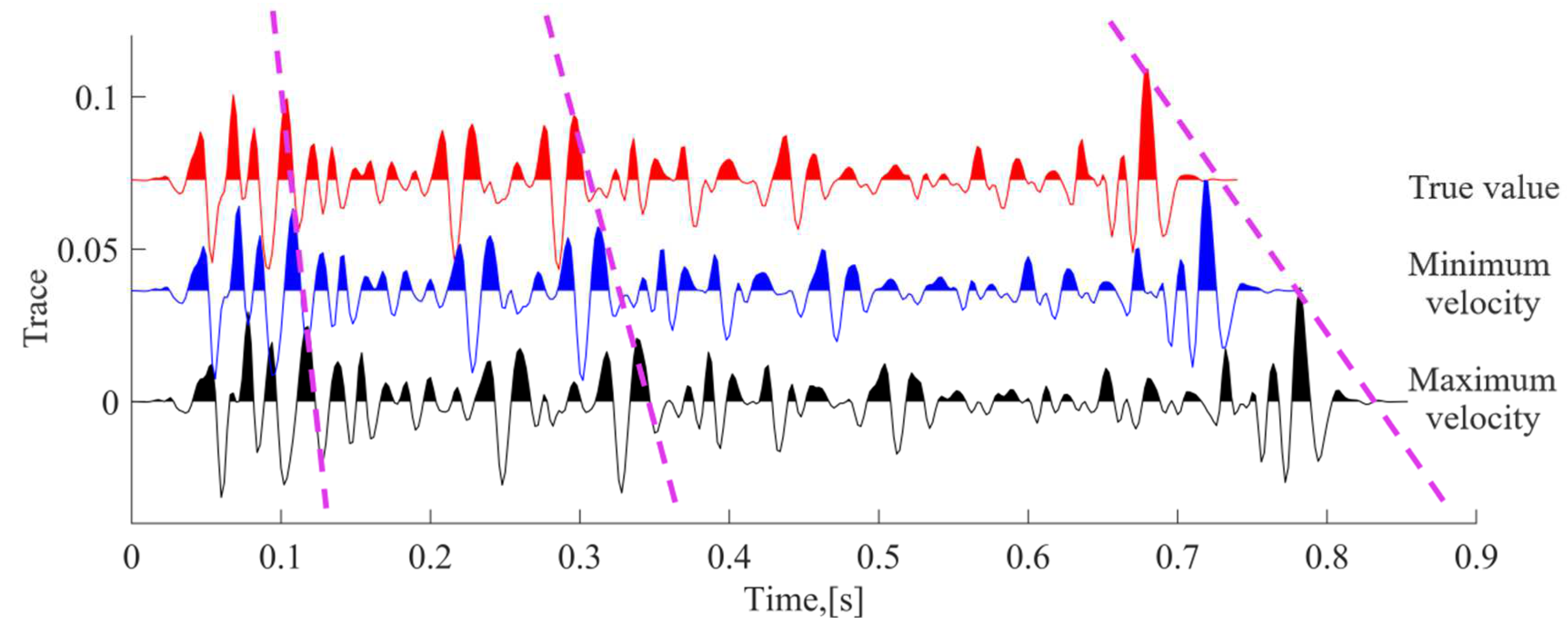
Then, the constant Q model is applied for the velocity dispersion correction. The results are shown in Figure 8. For the maximum velocity of the constant Q model, the synthetic data are similar to the real data. For the minimum velocity, as the values are smaller than those of logging velocity, the synthetic data stretch obviously, especially for the data after 0.4 s.
The SLS model is then applied and shown in Figure 9. As the velocity shows much smaller values in Figure 6a, the synthetic data show much more stretch than both the constant Q model and the Backus averaging method. The stretch can be seen starting from 0.2 s, and it becomes larger at 0.4 s. The stretch is largest at 0.9 s. The whole length of the data is 1.2 s.
4. Real Data Application
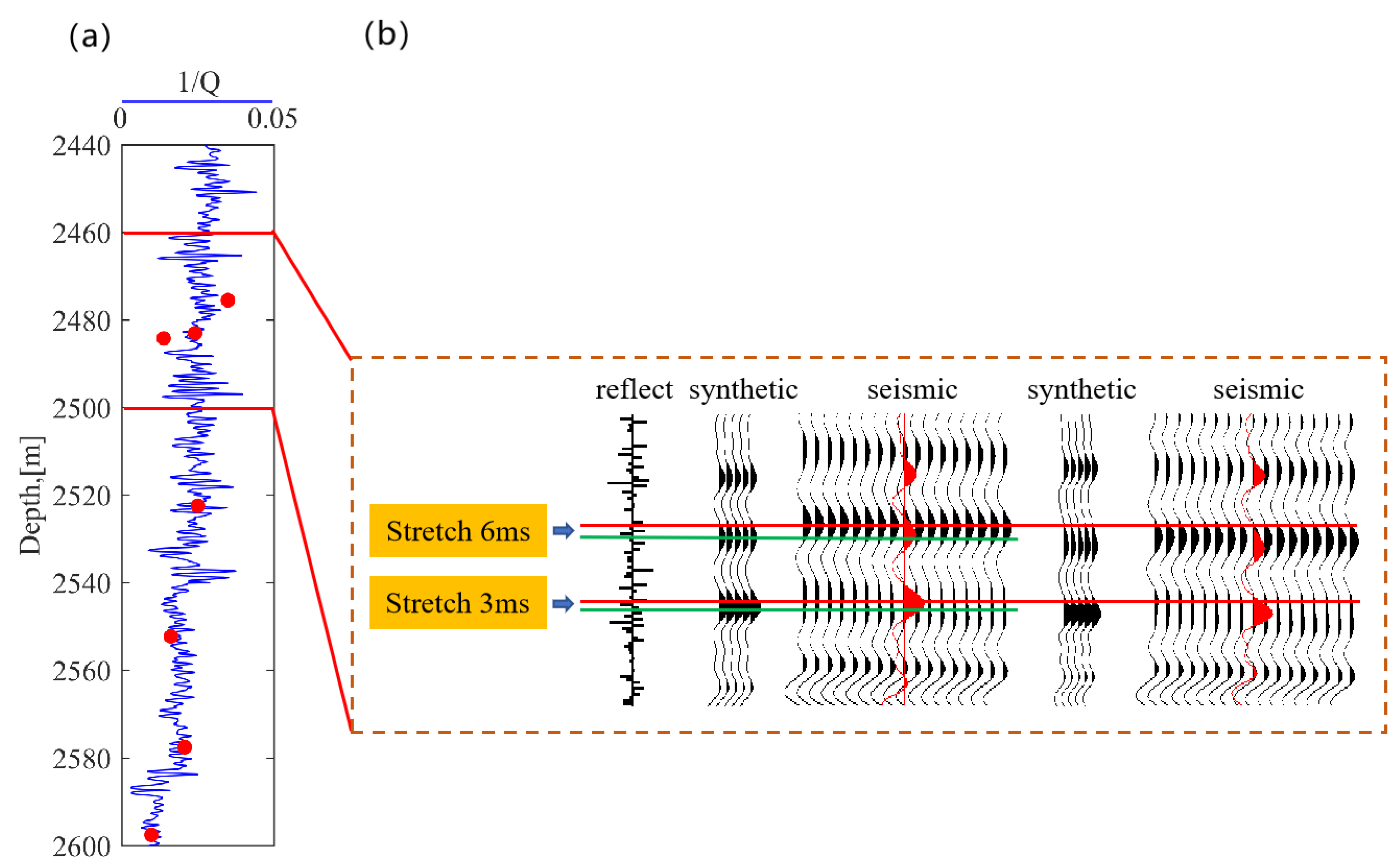
The proposed method is then applied to field data acquired in northern China. The Q−1 results are calculated using logging data by the pore fluid dissolution model. Figure 10a shows the Q−1 results at 60 Hz of this model in the depth from 1500 m to 2500 m. The results match well with the Q−1 measurements from the core data. The velocity is then upscaled by the SLS model. Figure 10b shows the well-to-seismic calibration before and after using velocity dispersion results from the SLS method as guidance for stretching the events. The event at 1900 ms is fixed, and the event at 1820 ms is stretched 5 ms. The event at 1740 ms is stretched 8 ms with the event at 1820 ms fixed. The corresponding velocity dispersion is calculated as roughly 7% and 4%, which is consistent with that of the SLS model. The upscaled velocity is useful for well-to-seismic calibration and makes the correction more reasonable.
5. Discussion
The Squirt model and the Pride model are not suitable for predicting the attenuation of rocks containing micro-pores at the seismic frequency band. The energy loss caused by fluid flow is neglectable, and gas dissolution and exsolution become the dominant attenuation mechanisms.
Although the conventional constant Q model is widely accepted, it will not predict accurate velocity dispersion when the corner frequency occurs in the seismic frequency band. For the same rock properties, the velocity range differs from that of the pore fluid dissolution model. The Backus averaging method almost results in a similar velocity range to that of real data. The size of the window chosen will not improve accuracy of velocity. Neither of these two methods are suitable for upscaling. The SLS model is suitable for upscaling the pore fluid dissolution model. The velocity dispersion and attenuation curve can be well modeled by the SLS model for different porosity and gas saturation cases.
Synthetic seismic data generated by using velocities calculated by these methods show obvious difference. Due to similar velocity range from the Backus averaging method, the events in the synthetic seismic data show little stretch. The constant Q model underestimates the velocity dispersion, and thus, the synthetic seismic data show little stretch until 0.4 s. The attenuation becomes observable because of the accumulation of the attenuation effect. The SLS model reasonably predicts the attenuation, and the synthetic seismic data show obvious difference from the traces generated by using logging velocity. When choosing a rock physical model for well-to-seismic calibration, one needs to consider the geology, geochemistry, and core data analysis report, and then select the appropriate rock physics model and update the parameters in the model.
6. Results
In this paper, an appropriate rock physical model is introduced, which can be used in seismic-to-well calibration. For rocks contains micro-pores, the pore fluid dissolution model is suitable for predicting the attenuation in the seismic frequency band. Compared with conventional methods, such as the constant model and the Backus averaging method, the SLS model can be chosen as the appropriate model for upscaling the pore fluid dissolution model. The introduced model can be used for seismic-to-well calibration. Both the synthetic seismic data and the field data test demonstrated the feasibility and accuracy of the proposed method.
Author Contributions
Methodology, Z.J. and X.Z.; Writing—review and editing, W.W.; Supervision, Y.S. All authors have read and agreed to the published version of the manuscript.
Funding
The study was conducted in accordance with the National Natural Science Foundation of China (grant no. 41930431).
Data Availability Statement
Not applicable.
Acknowledgments
The authors are grateful to the National Natural Science Foundation of China (grant no. 41930431).
Conflicts of Interest
The authors declare no conflict of interest.
References
- Pride, S.R.; Berryman, J.G.; Harris, J.M. Seismic attenuation due to wave-induced flow. J. Geophys. Res. Solid Earth 2004, 109, 1–19. [Google Scholar] [CrossRef]
- Müller, T.M.; Gurevich, B.; Lebedev, M. Seismic wave attenuation and dispersion resulting from wave-induced flow in porous rocks—A review. Geophysics 2010, 75, A147–A175. [Google Scholar] [CrossRef]
- Dvorkin, J.; Mavko, G.; Nur, A. Squirt flow in fully saturated rocks. Geophysics 1995, 60, 97–107. [Google Scholar] [CrossRef]
- White, J.E. Computed seismic speeds and attenuation in rock with partial gas saturation. Geophysics 1975, 40, 224–232. [Google Scholar] [CrossRef]
- White, J.E.; Mikhaylova, N.G.; Lyakhovitskiy, F.M. Low-frequency seismic waves in fluid-saturated layered rocks. Phys. Solid Earth 1975, 11, 654–659. [Google Scholar] [CrossRef]
- Johnson, D.L. Theory of frequency dependent acoustics in patchy-saturated porous media. Geology 2001, 110, 682–694. [Google Scholar] [CrossRef] [Green Version]
- Tisato, N.; Quintal, B.; Chapman, S.; Podladchikov, Y.; Burg, J.P. Bubbles attenuate elastic waves at seismic frequencies: First experimental evidence. Geophys. Res. Lett. 2015, 42, 3880–3887. [Google Scholar] [CrossRef]
- Tisato, N.; Madonna, C. Attenuation at low seismic frequencies in partially saturated rocks: Measurements and descriptions of a new apparatus. J. Appl. Geophys. 2012, 86, 44–53. [Google Scholar] [CrossRef]
- Tisato, N.; Quintal, B. Measurements of seismic attenuation and transient fluid pressure in partially saturated Berea sandstone: Evidence of fluid flow on the mesoscopic scale. Geophys. J. Int. 2013, 195, 342–351. [Google Scholar] [CrossRef]
- Chapman, N.; Quintal, S.; Tisato, B.; Holliger, K. Frequency scaling of seismic attenuation in rocks saturated with two fluid phases. Geophys. J. Int. 2017, 208, 221–225. [Google Scholar] [CrossRef]
- Sams, M.S.; Wolliamson, P.R. Backus averaging, scattering and drift. Geophys. Prospect. 1994, 42, 541–564. [Google Scholar] [CrossRef]
- Cao, D. The upscaling method of the well logging data based on Backus equivalence average method. Geophys. Prospect. Pet. 2015, 54, 105–111. [Google Scholar]
- Dong, E.Q.; Liu, G.Z.; Zhang, Z.P.; Chen, H.Z. Resampling of Logging Data and Matching of Synthetic Seismogram with Seismic Trace by Multiresolution Analysis. WLT 1999, 23, 264–267. [Google Scholar]
- Yang, W. A resonance Q model for viscoelastic rocks. Acta Geophys. Sin. 1987, 30, 399–411. [Google Scholar]
- Ba, J.; Jm, C.; Cao, H.; Du, Q.Z.; Yuan, Z.Y.; Lu, M.H. Velocity dispersion and attenuation of P waves in partially-saturated rocks: Wavepropagation equations in double-porosity medium. Chin. J. Geophys. 2012, 55, 219–231. (In Chinese) [Google Scholar]
- Wang, Z.; Sun, Y.; Xiao, Y. Full-frequency band velocity prediction model and its application on seismic reservoir prediction. Geology 2011, 73, 23–26. [Google Scholar]
- Picotti, S.; Carcione, J.M.; Rubino, J.G.; Santos, J.E.; Cavallini, F. A viscoelastic representation of wave attenuation in porous media. Comput. Geosci. 2010, 36, 44–53. [Google Scholar] [CrossRef]
- Wang, E.; Carcione, J.M.; Ba, J. Wave simulation in double-porosity media based on the Biot-Rayleigh theory. Geophysics 2019, 84, WA11–WA21. [Google Scholar] [CrossRef] [Green Version]
- Zhang, B.; Yang, D.; Cheng, Y.; Zhang, Y. A unified poroviscoelastic model with mesoscopic and microscopic heterogeneities. Geology 2019, 64, 1246–1254. [Google Scholar] [CrossRef] [Green Version]
- Picotti, S.; Carcione, J.M. Numerical simulation of wave-induced fluid flow seismic arrenuation based on the Cole-Cole model. Geology 2017, 142, 134–145. [Google Scholar]
- Lu, J.F.; Hanyga, A. Numerical modelling method for wave peopagation in a linear viscoelastic medium with singulat memory. Grophysical J. Int. 2004, 159, 688–702. [Google Scholar] [CrossRef] [Green Version]
- Bano, M. Modelling of GPR waves for lossy media obeying a complex power law of frequency for dielectric permittivity. Geophys. Prospect. 2004, 52, 11–26. [Google Scholar] [CrossRef] [Green Version]
- Hagin, P.N.; Zoback, M.D. Viscous deformation of unconsolidated reservoir sands—Part 2: Linear viscoelastic models. Geophysics 2004, 69, 742–751. [Google Scholar] [CrossRef]
- Toverud, T.; Ursin, B. Comparison of seismic attenuation models using zero-offset vertical seismic profiling (VSP) data. Geophisics 2005, 70, F17–F25. [Google Scholar] [CrossRef]
- Sacchi, M.D. Reweighting strategies in seismic deconvolution. Geophys. J. Int. 1997, 129, 651–656. [Google Scholar] [CrossRef] [Green Version]
- Rickett, J. Integrated estimation of interval-attenuation distributions. Geophysics 2006, 71, A19–A23. [Google Scholar] [CrossRef]
Figure 1.
Procedures of the proposed well-to-seismic calibration method.

Figure 2.
Comparison of velocity dispersion and attenuation calculated by three rock physics models. (a) Pore fluid dissolution model, (b) Squirt model and (c) Pride model. The blue solid line is the P wave velocity, and the red dash line is attenuation.
Figure 2.
Comparison of velocity dispersion and attenuation calculated by three rock physics models. (a) Pore fluid dissolution model, (b) Squirt model and (c) Pride model. The blue solid line is the P wave velocity, and the red dash line is attenuation.

Figure 3.
Comparison of velocity dispersion calculated by using the pore fluid dissolution model, the SLS model and the constant Q model. (a) Porosity 0.04 and gas saturation 0.25%, (b) Porosity 0.06 and gas saturation 0.25%, (c) Porosity 0.08 and gas saturation 0.25%, (d) Porosity 0.08 and gas saturation 0.15%, (e) Porosity 0.08 and gas saturation 0.2%, (f) Porosity 0.08 and gas saturation 0.25%. The two red solid curves are the results from the pore fluid dissolution model, the dash blue curves are from the SLS model, and the other dash curves (orange curve and cyan curve) are from the constant Q model.

Figure 4.
Comparison of 1/Q curves from the pore fluid dissolution model and the SLS model. The red solid curve is the pore fluid dissolution model, and the dash blue curve is the SLS mode. (a) Porosity 0.04 and gas saturation 0.25%, (b) Porosity 0.06 and gas saturation 0.25%, (c) Porosity 0.08 and gas saturation 0.25%, (d) Porosity 0.08 and gas saturation 0.15%, (e) Porosity 0.08 and gas saturation 0.2%, (f) Porosity 0.08 and gas saturation 0.25%.

Figure 5.
P_wave velocity calculated by using the Backus averaging method. The red solid curve is the real data, and the blue dash curve is the result from the Backus averaging method. (a) 16 samples in a window, (b) 8 samples in a window, (c) 4 sample in a window.
Figure 5.
P_wave velocity calculated by using the Backus averaging method. The red solid curve is the real data, and the blue dash curve is the result from the Backus averaging method. (a) 16 samples in a window, (b) 8 samples in a window, (c) 4 sample in a window.

Figure 6.
Velocity variation from the pore fluid dissolution model and the constant Q model. The orange area is the velocity range of the constant Q model. The cyan area is the velocity range of the pore fluid dissolution model. (a) Porosity ranges from 0.04 to 0.08, gas saturation is 0.25%, (b) porosity is 0.08, gas saturation ranges from 0.15% to 0.25%.

Figure 7.
Comparison of synthetic seismic data by using upscaled velocity from three different sizes of sample window using the Backus averaging method.
Figure 7.
Comparison of synthetic seismic data by using upscaled velocity from three different sizes of sample window using the Backus averaging method.

Figure 8.
Comparison of synthetic seismic data by using upscaled velocity from the maximum and minimum velocity of constant Q model in Figure 6a.
Figure 8.
Comparison of synthetic seismic data by using upscaled velocity from the maximum and minimum velocity of constant Q model in Figure 6a.

Figure 9.
Comparison of synthetic seismic data by using upscaled velocity from the maximum and minimum velocity of the SLS model in Figure 6a.
Figure 9.
Comparison of synthetic seismic data by using upscaled velocity from the maximum and minimum velocity of the SLS model in Figure 6a.

Figure 10.
(a) Comparison of Q−1 results by the WIGED model using logging data and data from core measurements. (b) Well-to-seismic calibration before and after using Q−1 results from the WIGED method as a guidance.
Figure 10.
(a) Comparison of Q−1 results by the WIGED model using logging data and data from core measurements. (b) Well-to-seismic calibration before and after using Q−1 results from the WIGED method as a guidance.


Table 1.
Parameters used in three rock physics models: the pore fluid dissolution model, the SLS model and the Pride model.
Table 1.
Parameters used in three rock physics models: the pore fluid dissolution model, the SLS model and the Pride model.
| Parameter | Symbol | Value | Unit |
|---|---|---|---|
| bulk modulus of oil | KO | 1.8 × 10⁹ | Pa |
| surface tension of gas | Sigma | 0.012 | Pa∙m |
| gas constant | R | 8.3144621 | m3∙Pa/K mol |
| Henry’s law constant of gas | KHpc | 4535 | Pa∙m3/mol |
| temperature | T | 350 | K |
| gas diffusion coefficient in water | DW | 1.00 × 10⁻⁸ | m2/s |
| gas solubility | S1 | 4535 | Pa∙m3/mol |
| initial pressure | Pi | 2.00 × 10⁷ | Pa |
| delta pressure | dP | 100 | Pa |
| water viscosity | visc_f | 1.00 × 10⁻³ | Pa∙s |
| CO2 viscosity | visc_g | 4.80 × 10⁻⁵ | Pa∙s |
| water density | rho_w | 840 | kg/m3 |
| gas density | rho_g | 119 | kg/m3 |
| CH4 viscosity | visc_g | 6.00 × 10⁻⁶ | Pa∙s |
| oil viscosity | visc_f | 8.00 × 10⁻⁴ | Pa∙s |
| high pressure | Ph | 2.00 × 10⁷ | Pa |
| initial radius of bubble | r | 5.00 × 10⁻⁶ | m |
| water saturation | Sat | 1.50 × 10⁻³ | unitless |
| porosity | phi | 6.00 × 10⁻² | unitless |
| mineral content of sand | Sand | 0.35 | unitless |
| mineral content of clay | Clay | 0.65 | unitless |
| Poisson ratio | pois | 0.14 | unitless |
| bulk modulus of the gas | Kg | 1.00 × 10⁴ | Pa |
| permeability | perm | 1.00 × 10⁻¹² | m2 |
Disclaimer/Publisher’s Note: The statements, opinions and data contained in all publications are solely those of the individual author(s) and contributor(s) and not of MDPI and/or the editor(s). MDPI and/or the editor(s) disclaim responsibility for any injury to people or property resulting from any ideas, methods, instructions or products referred to in the content. |
© 2022 by the authors. Licensee MDPI, Basel, Switzerland. This article is an open access article distributed under the terms and conditions of the Creative Commons Attribution (CC BY) license (https://creativecommons.org/licenses/by/4.0/).
Share and Cite
MDPI and ACS Style
Jin, Z.; Zheng, X.; Shi, Y.; Wang, W. Study on Seismic Attenuation Based on Wave-Induced Pore Fluid Dissolution and Its Application. Appl. Sci. 2023, 13, 74. https://0-doi-org.brum.beds.ac.uk/10.3390/app13010074
AMA Style
Jin Z, Zheng X, Shi Y, Wang W. Study on Seismic Attenuation Based on Wave-Induced Pore Fluid Dissolution and Its Application. Applied Sciences. 2023; 13(1):74. https://0-doi-org.brum.beds.ac.uk/10.3390/app13010074
Chicago/Turabian StyleJin, Ziqi, Xuelin Zheng, Ying Shi, and Weihong Wang. 2023. "Study on Seismic Attenuation Based on Wave-Induced Pore Fluid Dissolution and Its Application" Applied Sciences 13, no. 1: 74. https://0-doi-org.brum.beds.ac.uk/10.3390/app13010074
Note that from the first issue of 2016, this journal uses article numbers instead of page numbers. See further details here.