Magnitude and Similarity Based Variable Rate Filter Pruning for Efficient Convolution Neural Networks

Abstract

The superior performance of the recent deep learning models comes at the cost of a significant increase in computational complexity, memory use, and power consumption. Filter pruning is one of the effective neural network compression techniques suitable for model deployment in modern low-power edge devices. In this paper, we propose a loss-aware filter Magnitude and Similarity based Variable rate Filter Pruning (MSVFP) technique. We studied several filter selection criteria based on filter magnitude and similarity among filters within a convolution layer, and based on the assumption that the sensitivity of each layer throughout the network is different, unlike conventional fixed rate pruning methods, our algorithm using loss-aware filter selection criteria automatically finds the suitable pruning rate for each layer throughout the network. In addition, the proposed algorithm adapts two different filter selection criteria to remove weak filters as well as redundant filters based on filter magnitude and filter similarity score respectively. Finally, the iterative filter pruning and retraining approach are used to maintain the accuracy of the network during pruning to its target float point operations (FLOPs) reduction rate. In the proposed algorithm, a small number of retraining steps are sufficient during iterative pruning to prevent an abrupt drop in the accuracy of the network. Experiments with commonly used VGGNet and ResNet models on CIFAR-10 and ImageNet benchmark show the superiority of the proposed method over the existing methods in the literature. Notably, VGG-16, ResNet-56, and ResNet-110 models on the CIFAR-10 dataset even improved the original accuracy with more than 50% reduction in network FLOPs. Additionally, the ResNet-50 model on the ImageNet dataset reduces model FLOPs by more than 42% with a negligible drop in the original accuracy.

1. Introduction

Deep neural networks (DNNs) have achieved remarkable performance in many applications such as object detection, image segmentation, medical imaging, surveillance systems, etc. Mainly the emergence of fast graphics processing units (GPUs) with huge memory bandwidth and computational power enabled the development of accurate and large-size DNNs. The number of layers in modern DNNs with wider and deeper architectures can reach tens of thousands with billions of parameters [1]. However, it comes at the cost of increased model size, memory use, power consumption, and heavy computation requirements. Bianco et al. [2] presents a nice ball chart reporting evolution of DNN models in terms of accuracy on the ImageNet-1k [3] validation set with respect to the computational complexity over the past few years. It is challenging to deploy such complex DNNs in portable devices with limited resources (e.g., memory, bandwidth, energy, etc.). Therefore, in order to deploy those models on resource-constrained low-power edge devices (e.g., mobile phones, smart wearable devices, drones, robots, etc.), it is essential to reduce the computational cost and storage demand of modern DNNs. To achieve this goal, several methods have been developed including model compression, neural architecture search (NAS)  [4,5], hardware optimization [6,7], and algorithm hardware co-design [8,9]. Among them, CNN model compression can be achieved with several techniques such as pruning [10,11,12,13,14,15,16], quantization [17,18,19], knowledge distillation [20,21], and tensor decomposition [22,23].

Pruning is a promising approach for neural network compression that can be divided into two main categories, weight pruning (e.g., [10,11]), and filter pruning (e.g., [13,24,25]). Weight pruning removes the individual entries in the filter or connection in fully connected layers and the resulting network is unstructured and sparse. Filter pruning, on the other hand, removes the unimportant or redundant filters from the network producing slimmed yet structured model, still permitting dense matrix operations and suitable for any off-the-shelf general-purpose hardware and libraries. Although weight pruning significantly reduces the model size, specialized hardware and software are required to leverage the full capacity of the resulting non-structured sparse model. In this paper, we focus on filter pruning, which is also a preferred method for convolution neural network (CNN) model compression and acceleration (FLOPs reduction) to provide a solution for model deployment in devices with low computing power and memory requirements.

The key to filter pruning is the selection and removal of the least important filters in terms of overall accuracy degradation. For this, we need to define the pruning policies, which include pruning criteria and pruning rate. Filter ranking with certain criteria [13,24], minimization of reconstruction error [26,27], and redundancy estimation using similarity calculation [15,16] are the three main branches of filter pruning. Pruning unimportant filters in terms of their magnitude via $l_1$-norm (Li et al. [24]) or $l_2$-norm (He et al. [13]) criteria is the most commonly used filter pruning criteria. Besides filter magnitude, filter similarity information is also an important filter selection criterion for removing redundant filters. This paper utilizes both the filter magnitude and similarity information to remove both unimportant and replaceable filters. It is important to determine the appropriate pruning rate for each layer. Most existing methods use a single pruning rate for different layers. However, the convolution layers in CNNs are not independent and filters in different layers have different distributions and importance, therefore the fixed-rate pruning is not suitable. The variable rate filter pruning across different convolutional layers is proved to be an effective method in reconstructing the original accuracy. In this paper, we also use different pruning rates for each convolution layer, which is in fact automatically identified by the proposed iterative pruning algorithm. The main focus of any pruning algorithm is to minimize network loss while removing as many filters as possible. Consequently, in recent years loss-aware filter pruning methods are gaining popularity. The proposed pruning algorithm, in every pruning iteration, globally searches for the set of filters from the whole network which is least important in terms of overall network loss. The pruning algorithms presented by He et al. [13,15,16] claim that soft filter pruning, i.e., keeping track of pruned filters and updating them during training, has proven to be more effective as compared to the conventional train-prune-retrain pipeline. But, the disadvantage is that filter selection and pruning from the original network should be performed in every training epoch resulting in increased computational cost. Therefore in this paper, we used a hard filter pruning approach, i.e., whenever the filter is selected for pruning, the selected filter along with its connections in the network are permanently removed. The advantage of this approach is that once the pruning is completed the resulting slimmed network with reduced complexity can be used for final retraining. Moreover, the proposed technique is evaluated on relatively simple VGGNet to complex ResNet architectures using CIFAR-10 and ImageNet benchmark datasets.

The main contributions of this paper are summarized as follows:

• We analyze several magnitudes and similarity based filter selection criteria and utilized both criteria in designing the pruning algorithm. The filters are pruned in a hard manner, i.e., if the filter is selected for pruning, it is permanently removed and the network is rearranged for further processing.
• Loss-aware variable rate pruning is used across different layers of the network which is more effective compared to fixed-rate pruning. The optimal pruning rate for each layer is automatically identified.
• To show the effectiveness of the proposed pruning algorithm the commonly used VGGNet and ResNet are evaluated on CIFAR-10 and ImageNet benchmark datasets. Detailed analysis of the pruning and retraining process shows how to reduce the overall cost of the pruning algorithm.

The remainder of this paper is organized as follows: Section 2 describes some relevant prior work in network pruning. Then, we present a detailed process of the proposed pruning algorithm, MSVFP, in Section 3. This section includes several filter selection criteria along with a detailed pruning algorithm. In Section 4, a discussion on the experimental evaluation of our method in comparison with state-of-the-art (SOTA) methods is presented. We finally conclude the proposed algorithm in Section 5. Additionally, the implementation code for this paper has been open sourced and available online (https://github.com/ghimiredhikura/MSVFP-FilterPruning, accessed on 6 December 2022).

2. Related Works

The key idea in pruning is to remove the least important weights, filters, or even a whole layer from the CNNs. The weight or connection pruning eliminates the unimportant connections from the network resulting in an unstructured sparse network [10,11,12,28]. The filter or channel pruning eliminates the entire filter or channel retaining the original structure of the network [13,14,16,24,25,26,27,29]. In contrast to filter pruning, sparse networks after weight pruning require specialized hardware or software in order to achieve practical acceleration. Besides conventional weight and filter pruning, the recently developed $1\times N$ pruning scheme by Lin et al. [30] removes the consecutive N output kernels with the same input channels in order to accelerate the neural network via parallelized block-wise vectorized operations on general central processing units (CPUs). The joint optimization techniques presented by Wang et al. [31] and Han et al. [10] utilize other compression techniques such as quantization and NAS along with pruning for better compression results. A recent state of approaches to pruning in the literature is presented by Blalock et al. [32], in which authors also provide the standardized benchmark and matrices to compare the pruning results among different pruning schemes.

2.1. Weight Pruning

The early work on weight pruning prunes the weights below the threshold using iterative connection pruning and fine-tuning. The pioneering work by LeCun et al. [33] utilizes the second derivatives (Hessian matrix) of the loss function to prune each non-essential weight. In the era of deep learning, the popular work on weight pruning by Han et al. [28] demonstrates that plenty of weights below the threshold can be simply removed from DNNs to achieve a significant compression ratio. The lottery ticket hypothesis (LTH), presented by Frankle et al. [11], is another popular approach in weight pruning that shows that dense, randomly-initialized neural network contains subnetworks (“winning tickets”) when trained in isolation. Specifically, each pruned subnetwork is trained from scratch, but the weights are initialized as the same initial weights used in the original network. Several variants of LTH, such as Generalized LTH  [34], Dual LTH [35], etc., are also developed for weight pruning. While Han et al. [10,28] uses the constant global magnitude threshold for weight pruning in the whole network, Ding et al. [12] uses the global compression ratio to find the appropriate per-layer sparsity ratio. Aghasi et al. [36] formulated the connection pruning as a convex optimization problem.

Although weight pruning can remove a significant number of connections without damaging the original capacity of the network, it requires specialized hardware or software to speed up inference. Due to irregular sparsity in weight matrices, it has limited applications on general-purpose hardware.

2.2. Filter Pruning

The main importance of filter pruning is to define some criteria to select unimportant filters. Li et al. [24] calculate filter magnitude in terms of $l_1$-norm is used to remove low-norm filters. Again, He et al. [13] used $l_2$-norm to remove the filters in a soft manner and suggest that $l_2$-norm criteria work slightly better than $l_1$-norm criteria. Another soft filter pruning, FPGM [15], prunes redundant filters using filter Euclidean similarity criteria rather than pruning less important filters using magnitude criteria. A similar soft pruning technique presented by He et al. [16] adaptively selects the most suitable criteria for pruning via a meta-attribute of the network at the current state. The global filter ranking algorithm, LeGR [37], can remove the required amount of bottom-ranked filters to achieve a target pruning rate. ThiNet [26] formulated pruning as an optimization problem, which prunes filters in the current layer and minimizes the reconstruction error in the next layer. In contrast to ThiNet [26], NISP [27] focus on minimizing the reconstruction error in the final response layer while pruning filters in the current layer. He et al. [14] trained the differentiable criteria sampler to learn the most appropriate pruning criteria for different layers. Also, Bayesian optimization-based variable rate one-shot filter pruning is recently presented by Kim et al. [29], in which optimal pruning rates for each layer are automatically identified. Recently, GFI-AP [25] extensively studies the filter importance criteria for each layer and proposes that variable rate pruning across convolution layers outperforms fixed rate filter pruning. Instead of selecting pruning filters using magnitude or similarity criteria, Lin et al. [38] formulated the information preserving of pretrained CNN filters as a matrix sketch problem, but they still use the fixed rate pruning for all pruning layers in the network.

Filter pruning or structured pruning does not have limitations on specialized hardware or software as entire filters are pruned and the original structure of the network still remains intact. Therefore filter pruning is more favorable as compared to weight pruning.

3. Pruning Methodology

In this section, we will introduce several filter selection criteria, the overall algorithm, and the tools used in the proposed technique. Researchers tend to use either filter magnitude-based criteria or filter similarity-based criteria for filter selection and removal. In this paper, we take advantage of both criteria and at the same time, we use automatically calculated loss-aware dynamic pruning rates for each layer in the convolutional network. The following subsections will describe each of these steps in detail.

3.1. Preliminaries

In this paper, we used similar mathematical notations as in [16]. Let us assume a neural network has L layers. $N_i$ and $N_{i+1}$ are the number of input and output channels in the $i_{th}$ convolution layer, respectively. Suppose ${\mathcal{F}}_{i,j}\in {\mathbb{R}}^{N_i\times K\times K}$ is the $j_{th}$ filter in the $i_{th}$ convolution layer, where K is the kernel size of the filter. Therefore, for the $i_{th}$ layer, network consists set of filters denoted as ${\mathcal{F}}_{i,j},1\le j\le N_{i+1}$ and parameterized by ${\mathcal{W}}^{\left(i\right)}\in {\mathbb{R}}^{N_{i+1}\times N_i\times K\times K},1\le i\le L$. For simplicity, let us represent all 3-D filters ${\mathcal{F}}_{i,j}$ in $i_{th}$ convolution layer as one dimensional vector $\mathcal{X}\in {\mathbb{R}}^{N_{i+1}\times M_i}$, which means in $i_{th}$ convolution layer there are $N_{i+1}$ filter vectors and each vector has length $M_i=N_i\times K\times K$.

3.2. Filter Selection Criterion

In the proposed algorithm our main focus is to iteratively select and remove the most unimportant group of filters from convolution layers so that it will have minimal effect on the accuracy loss during inference. Therefore at first, we will need to rank the importance of filters within a layer using information from the filter itself. The filter magnitude using norm or the measure of geometric similarity among filters are two widely used criteria to rank the filter’s importance. We studied several of those criteria as follows.

(a) Filter Magnitude. In the early days of weight pruning, i.e., unstructured pruning, researchers found that small weight values can be safely removed without hurting the network performance. The same goes for filter pruning, also known as structured pruning. The filter norm values are used to calculate the overall filter magnitudes. Li et al. [24] extensively demonstrated that filters with small norm values are less important as compared to large norm filters and they can be safely removed. In this paper, we also used filter norms to estimate filter magnitudes. If we represent $j_{th}$ filter ${\mathcal{X}}_j$ as $\mathit{x}\in {\mathbb{R}}^{1\times M_i}$, its $l_p$-norm is calculated as

$${\parallel {\mathcal{X}}_j\parallel }_p=\sqrt[{}^p]{\sum _{m=1}^{M_i}{|x_m|}^p}$$

(1)

Either $l_1$-norm or $l_2$-norm can be used to get the filter magnitude and filters with low norm values will be dropped during pruning.

(b) Filter Similarity. While filter magnitude using norm is a good measure for removing unimportant filters, the network still may contain unnecessary filters but with a large magnitude. He et al. [15,16] proposed that not only the filter magnitude but filter similarity scores can be used to rank filters for pruning. The filter that has the largest similarity score among all other filters in the layer can be safely removed because such a filter is considered redundant and the information loss due to the removal of such a filter can be easily recovered by the remaining filters in the layer. Therefore, in this paper, we also utilize the filter similarity measures in addition to norm-based magnitude criteria for removing unimportant filters. Here we studied three different filter similarity estimation methods having different properties from each other.

Euclidean Similarity. The similarity measurement using Euclidean distance depends upon the magnitude of two vectors. The Euclidean similarity between two filter vectors $\mathit{x}\in {\mathbb{R}}^{1\times M_i}$ and $\mathit{y}\in {\mathbb{R}}^{1\times M_i}$ is calculated as

$$D_{eucl}(\mathit{x},\mathit{y})=\sqrt{\sum _{m=1}^{M_i}{|x_m-y_m|}^2}$$

(2)

Cosine Similarity. Cosine similarity measures the cosign of angles between two vectors that determine if two vectors are pointing in the same direction. The Cosine similarity between two filter vectors $\mathit{x}\in {\mathbb{R}}^{1\times M_i}$ and $\mathit{y}\in {\mathbb{R}}^{1\times M_i}$ is calculated as

$$D_{cos}(\mathit{x},\mathit{y})=1-\frac{{\sum }_{m=1}^{M_i}\left(x_m\times y_m\right)}{{\sum }_{m=1}^{M_i}{x}_m^2\times {\sum }_{m=1}^{M_i}{y}_m^2}$$

(3)

Normalized Cross Correlation (NCC) Similarity. Unlike cosign similarity, NCC is invariant to scale and shift. In image processing, NCC is a good measure for template matching which is robust to exposure and lighting. Therefore, in this paper, NCC is also studied to measure the similarity between filters. The NCC similarity between two filter vectors $\mathit{x}\in {\mathbb{R}}^{1\times M_i}$ and $\mathit{y}\in {\mathbb{R}}^{1\times M_i}$ is calculated as

$$D_{ncc}(\mathit{x},\mathit{y})=1-\frac{1}{M_i}\sum _{m=1}^{M_i}\frac{(x_m-\mu {}_x\left)\right(y_m-\mu {}_y)}{\sigma {}_x\sigma {}_y}$$

(4)

where $\mu {}_x$, $\mu {}_y$ are the mean and $\sigma {}_x$, $\sigma {}_y$ are the standard deviation of vector $\mathit{x}$ and $\mathit{y}$.

The goal of filter selection using similarity criteria is to find a filter that is most similar to all other filters within the layer. The similarity score for each filter will be calculated using one of the similarity estimation methods described above. Let us consider we choose Euclidean distance (Equation (2)) to calculate the similarity value between two filter vectors. The final similarity score for $j_{th}$ filter is estimated as an average of similarity values with all other remaining filters in the layer. This score will be used to decide if we can remove this filter during pruning. Therefore, the similarity score for a $j_{th}$ filter in a $i_{th}$ convolutional can be formulated as

$$S\left({\mathcal{X}}_j\right)=\frac{{\sum }_{p=1,p\ne j}^{N_{i+1}}D({\mathcal{X}}_j,{\mathcal{X}}_p)}{N_{i+1}-1}$$

(5)

where $D({\mathcal{X}}_j,{\mathcal{X}}_p)$ is the similarity value between $j_{th}$ and $p_{th}$ filter calculated using Equations (2), or (3), or (4).

3.3. Pruning Algorithm

As stated earlier, at each pruning iteration, after selecting the set of unimportant filters using filter important estimation criteria, the pruning is carried out from the particular convolution layer in which network loss is minimal. This means we use a greedy search approach to find the optimal set of filters at each pruning iteration, which results in variable rate pruning for each layer. During pruning, in each pruning iteration, the loss estimation using the full training dataset is computationally expensive, therefore randomly sampled small subset of the training dataset is used for this purpose.

Given a dataset $\mathcal{D}$, ${\mathcal{D}}^{\prime }$ is the randomly sampled small subset of this dataset. We denote ${\mathcal{W}}^{\prime \left(i\right)}$ as the filter of the $i_{th}$ layer after pruning, and $N_{i+1}^{\prime }$, the number of filters after pruning. Now, the estimation of accuracy loss during each pruning step is denoted as $Loss\left({\mathcal{D}}^{\prime }\right|{\mathcal{W}}^{\prime })$. In each pruning iteration, we temporarily prune each layer and select the layer with minimal accuracy loss. The number of filters to be pruned in each step is calculated as $N_{i+1}\times {\alpha }_s$, where ${\alpha }_s$ is the step pruning rate. In order to avoid excessive pruning from the single convolutional layer, we limit the maximum pruning rate of a layer as ${\alpha }_{max}$. For example, if ${\alpha }_{max}=70\%$, at max $N_{i+1}\times 70\%$ filters can be pruned from $i_{th}$ convolutional layer.

The filter magnitude and filter similarity score are two different criteria for measuring filter importance. In our paper, we take advantage of both criteria to get optimal accuracy of the model after pruning. We design the pruning algorithm in such a way that we can input the partition rate for desired pruning ratio into two criteria. The ultimate goal of network pruning is to reduce the FLOPs in the network. Therefore instead of filter pruning rate, our algorithm directly takes the FLOPs reduction rate ($\mathcal{P}$) as the desired pruning rate and pruning is carried out iteratively until the desired FLOPs reduction rate is achieved. If $f_{flop}\left({\mathcal{W}}^{\prime }\right)$ is the total FLOPs of pruned network ${\mathcal{W}}^{\prime }$, the FLOPs reduction rate over the original network is calculated as

$${\mathcal{P}}^{\prime }=1-\frac{f_{flop}\left({\mathcal{W}}^{\prime }\right)}{f_{flop}\left(\mathcal{W}\right)}$$

(6)

At first, unimportant, low-magnitude filters are pruned using norm-based criteria (e.g., $l_1$-norm), and in the next step, redundant filters are pruned using similarity-based criteria (e.g., Euclidean similarity). The reason behind pruning low-magnitude filters at first is that the similarity criterion is able to remove redundant filters even if their magnitude is large. If the pruning weight for magnitude criteria is $w_{mag}$ among two criteria, a total of $\mathcal{P}\times w_{mag}$ FLOPs reduction is achieved using magnitude criteria, and the remaining $\mathcal{P}\times (1-w_{mag})$ FLOPs reduction is achieved using similarity criteria. Therefore according to the value of $w_{mag}$ we can decide what portion of filters are removed using filter norm magnitude criteria or filter similarity criteria to achieve the target pruning rate. For example, if we set $w_{mag}=0.5$, almost the same number of filters will be removed using each criterion.

The detailed pruning steps of the proposed approach are summarized in Algorithm 1. Given the training dataset ($\mathcal{D}$) and pretrained model ($\mathcal{W}$), the algorithm iteratively prunes a certain percentage of filters from each selected layer until the target FLOPs reduction rate is achieved. As we partition pruning among two filter selection criteria, if the current FLOPs reduction rate is in the range from 0 to $\mathcal{P}\times w_{mag}$ (Line 5), magnitude based pruning (Line 6–11) is used. During this process, the algorithm scans through each layer (Line 6) and temporarily prunes a small set of filters ($N_{i+1}\times {\alpha }_s$) in order to generate the set of candidate pruned models ${\mathcal{W}}^{*\left(i\right)}$ (Line 9). For each layer, we limit the maximum number of pruning filters to $N_{i+1}\times {\alpha }_{max}$ (Line 7) to avoid excessive pruning from a single convolution layer. Similarly, if the current FLOPs reduction rate is in the range from $\mathcal{P}\times w_{mag}$ to $\mathcal{P}$ (Line 12), the filter similarity based pruning (Line 13–18) is used to generate set of candidate pruned models. Now, for the current pruning iteration, the pruned model that has minimal accuracy loss among candidates is selected (Line 20) and pruning is made permanent. In order to prevent the large accuracy drop during pruning, after each ${\beta }_{\mathcal{P}}$ FLOPs reduction rate, the pruned model will be fine-tuned for a small number of epochs ($epoc{h}_{ft}$) (Line 22). Once desired pruning rate is achieved, the pruned model will be retrained for several epochs ($epoc{h}_{rtend}-epoc{h}_{rtstart}$) to get the final pruned model (Line 27).

Algorithm 1 Algorithm of MSVFP

Input: training data $\left(\mathcal{D}\right)$, pretrained model $\left(\mathcal{W}\right)$    1: Given: target FLOPs reduction rate ($\mathcal{P}$), step pruning rate (${\alpha }_s$), max pruning rate (${\alpha }_{max}$), weighted for magnitude criteria ($w_{mag}$), fine-tune FLOPs reduction interval (${\beta }_{\mathcal{P}}$), number of finetune epochs during pruning ($epoc{h}_{ft}$), final retrain start epoch number ($epoc{h}_{rtstart}$), final retrain end epoch number ($epoc{h}_{rtend}$)    2: Initialization:${\mathcal{W}}^{\prime }\leftarrow \mathcal{W}$, ${\mathcal{P}}^{\prime }\leftarrow 0$, ${\mathcal{P}}_{temp}^{\prime }\leftarrow 0$    3: Randomly sample dataset ${\mathcal{D}}^{\prime }$ from $\mathcal{D}$    4: while${\mathcal{P}}^{\prime }<\mathcal{P}$do    5:    if ${\mathcal{P}}^{\prime }\le \mathcal{P}\times w_{mag}$ then    6:      for $i\leftarrow 1$ to L do    7:         if $N_{i+1}^{\prime }\ge N_{i+1}\times {\alpha }_{max}$ then    8:           Calculate magnitude of filters using Equation (1) in ${\mathcal{W}}^{\prime \left(i\right)}$    9:           ${\mathcal{W}}^{*\left(i\right)}\leftarrow$ Prune $N_{i+1}\times {\alpha }_s$ filters with lowest magnitude values    10:         end if    11:      end for    12:    else    13:      for $i\leftarrow 1$ to L do    14:         if $N_{i+1}^{\prime }\ge N_{i+1}\times {\alpha }_{max}$ then    15:           Calculate similarity score of filters using Equation (5) in ${\mathcal{W}}^{\prime \left(i\right)}$    16:           ${\mathcal{W}}^{*\left(i\right)}\leftarrow$ Prune $N_{i+1}\times {\alpha }_s$ filters with highest similarity scores    17:         end if    18:      end for    19:    end if    20:    ${\mathcal{W}}^{\prime }\leftarrow \underset{{\mathcal{W}}^{*\left(i\right)}}{argmin}(Loss\left({\mathcal{D}}^{\prime }\right|{\mathcal{W}}^{*\left(i\right)})$    21:    Calculate ${\mathcal{P}}^{\prime }$ using Equation (6)    22:    if ${\mathcal{P}}^{\prime }-{\mathcal{P}}_{temp}^{\prime }\ge {\beta }_{\mathcal{P}}$ then    23:      Fine-tune ${\mathcal{W}}^{\prime }$ to recover weights ($epoch\leftarrow 1$ to $epoc{h}_{ft}$)    24:      ${\mathcal{P}}_{temp}^{\prime }\leftarrow {\mathcal{P}}^{\prime }$    25:    end if    26: end while    27: Re-train ${\mathcal{W}}^{\prime }$ until convergence ($epoch\leftarrow epoc{h}_{rtstart}$ to $epoc{h}_{rtend}$)  Output: pruned model $\left({\mathcal{W}}^{\prime }\right)$

4. Experimental Results

4.1. Experimental Settings

Datasets and Baseline Architectures. To demonstrate the effectiveness and performance of our pruning technique we conducted experiments on two commonly used datasets, CIFAR-10 [39] dataset, and ImageNet [3] benchmark dataset. The CIFAR-10 dataset contains 50 k training images and 10k validation images of size $32\times 32$ categorized into 10 classes. The ImageNet dataset contains 1.28 million training images and 50 k validation images categorized into 1k classes. We mainly focus on pruning the multi-branch residual network structures (ResNet [40]) and evaluated them on both CIFAR-10 and ImageNet datasets. Moreover, we have also pruned a relatively easy single-branch VGGNet [41] and evaluated it on the CIFAR-10 dataset. The VGGNets are based on the most essential features of CNN and contain sequential convolutions. For example, the VGG-16 network used in our experiment consists of 16 sequential convolutional layers and three fully connected layers. On the other hand, ResNet is designed with residual blocks. The concept of shortcut connection in residual blocks is the main strength of this type of network solving the vanishing gradient problem and allowing us to design deeper architectures.

Training Setting. For training ResNet and VGGNet on the CIFAR-10 dataset, we use the same training settings as in [42,43] and [15,24], respectively. Training ResNet on the ImageNet dataset we used the default parameter setting from He et al. [40] and the same data augmentation strategies used in official PyTorch [44] examples. After pruning, while retraining the pruned network, the starting learning rate is set to $10\%$ of the original learning rate, while keeping the other settings the same as in baseline training. Although the same number of training epochs are used in retraining the pruned network, we empirically found that pruned network converges in less number of epochs as compared to baseline training.

Pruning Setting. We use the deep learning framework PyTorch [44] along with a structural pruning tool developed by Fang [45] for pruning and fine-tuning the neural network. In every pruning iteration, the pruned filters are permanently removed and the network is rearranged for the next pruning iteration. The maximum pruning rate for each layer is empirically set to ${\alpha }_{max}=0.7$, i.e., in each layer we limit the maximum number of pruned filters to $70\%$ of the original number of filters in that layer. This value makes sense because by allowing too many filters to be removed from a single layer it will be difficult to recover the baseline accuracy of the pruned model. Again, reducing the maximum limit to a smaller value will limit the freedom for filter selection from a suitable layer in the network as we will experiment with up to the $54\%$ FLOPs reduction rate. We set ${\alpha }_s=0.1$, which means, in each pruning iteration we empirically prune $10\%$ of the filters from the selected pruning layer. During pruning, after every ${\beta }_{\mathcal{P}}=0.3$ (i.e., $3\%$) network FLOPs reduction rate, the pruned network is fine-tuned for a small number of epochs, which ranges from 1 to 3. This makes sure that network accuracy will not drop abruptly during pruning which also helps the loss-aware filter selection to work effectively.

Evaluation Matrices. The primary goal of a structured pruning algorithm is to directly reduce the computational requirement of the model without requiring any specialized hardware. This can be achieved by reducing the required FLOPs of the model. The proposed algorithm directly takes the FLOPs reduction rate as the target pruning rate. Given the target pruning rate, average top-1 accuracy along with standard deviation from three experiments on the CIFAR-10 dataset is used to evaluate the capability of the pruning. As suggested by Joo et al. [46], we used both final accuracy and accuracy drop w.r.t. baseline accuracy for performance evaluation. In addition, we used average from scratches [46] with distinct baselines rather than using a single baseline while averaging the results from different experiments. Again, on the ImageNet dataset, both top-1 and top-5 accuracy are used to evaluate the performance. Unlike CIFAR-10 dataset, in the case of the ImageNet dataset, we report results from a single experiment in order to limit the time and resource requirements in training and pruning.

4.2. VGGNet on CIFAR-10

Table 1. Pruning VGGNet on the CIFAR-10 dataset using different filter selection criteria and a different number of fine-tune epochs. ’FT epochs’ means ’Fine-tune epochs’.

Method	${\mathit{w}}_{\mathit{mag}}$	Top-1 Acc (%)
		40 FT Epochs	80 FT Epochs	160 FT Epochs
Baseline	-	93.79 ± 0.23	93.79 ± 0.23	93.79 ± 0.23
Pruned ($l_1$-norm)	1.0	93.60 ± 0.14	93.71 ± 0.14	93.92 ± 0.01
Pruned (eucl)	0.0	93.60 ± 0.14	93.84 ± 0.06	93.92 ± 0.03
Pruned (cos)	0.0	93.48 ± 0.23	93.64 ± 0.12	93.69 ± 0.15
Pruned (ncc)	0.0	93.51 ± 0.15	93.69 ± 0.27	93.73 ± 0.07
Pruned ($l_1$-norm + eucl)	0.5	93.75 ± 0.06	93.89 ± 0.03	94.02 ± 0.04

Note that bold numbers in the table indicate the best result.

shows the result of pruning VGG-16 on the CIFAR-10 dataset achieving a 34% FLOPs reduction rate using different filter selection criteria. The first row in the table is the baseline accuracy of pretrained network before pruning. We experiment with the pruning of this pretrained network using different filter selection criteria and empirically found that norm magnitude and euclidean similarity criteria are effective in retaining the accuracy of the model. According to the provided $w_{mag}$ value in Algorithm 1 the proposed pruning algorithm will use either magnitude criteria or similarity criteria or a combination of both. From the Table 1, we can see that among similarity criteria, euclidean similarity produces a better result. The magnitude information seems to be the crucial information even in similarity-based filter selection criteria because cosine and NCC similarity are invariant to filter magnitude. The best result is obtained while removing half of the network FLOPs with $l_1$-norm criteria and another half with euclidean similarity criteria for the given FLOPs reduction rate. As we can see in the Table 1, the original accuracy of the pruned model is recovered with just 40 fine-tune epochs, and if we further increase the fine-tune epochs, the accuracy of the pruned model surpassed the baseline accuracy.

Table 2. Comparison of VGGNet pruning on the CIFAR-10 dataset.

Method	Baseline Top-1 Acc. (%)	Pruned Top-1 Acc. (%)	Top-1 Acc. Drop (%)	FLOPs (↓) (%)
PFEC [24]	93.58 ± 0.03	93.28 ± 0.03	0.30	34.2
FPGM [15]	93.58 ± 0.03	94.00 ± 0.13	−0.42	34.2
MFP [16]	93.58 ± 0.03	93.76 ± 0.08	−0.18	34.2
MSVFP(ours)	93.79 ± 0.23	94.02 ± 0.04	−0.23	35.1
MSVFP(ours)	93.79 ± 0.23	93.84 ± 0.08	−0.05	50.7

Note that bold numbers in the table indicate the best result.

shows comparison of accuracy results with other similar state-of-the-art pruning methods. With a similar pruning rate, the proposed algorithm achieved $94.02\%$ accuracy of the pruned network which is better as compared to results reported by PFEC [24], MFP [16], and FPGM [15]. Note that PFEC [24], and FPGM [15] use fixed-rate pruning while our method use loss-aware variable rate pruning. Furthermore, even after reducing the VGGNet FLOPs by more than $50\%$ using the proposed algorithm, the pruned network is still able to retain its original accuracy.

4.3. ResNet on CIFAR-10

At first, as shown in

Table 3. Pruning ResNet-20 on the CIFAR-10 dataset using different filter selection criteria.

Method	${\mathit{w}}_{\mathit{mag}}$	Top-1 Acc. (%)
Baseline	-	92.34 ± 0.09
Pruned ($l_1$-norm)	1.0	91.72 ± 0.15
Pruned (eucl)	0.0	91.61 ± 0.27
Pruned (cos)	0.0	90.76 ± 0.22
Pruned (ncc)	0.0	90.77 ± 0.27
Pruned ($l_1$-norm + eucl)	0.5	91.78  ±  0.17

Note that bold numbers in the table indicate the best result.

, we test our pruning algorithm on ResNet-20 using the CIFAR-10 dataset with different filter selection criteria while reducing network FLOPs by $54.5\%$. Similar to VGGNet pruning (Table 1), while pruning the ResNet-20 model (Table 3), using single filter selection criteria, we found that $l_1$-norm and euclidean similarity based criteria are on the top among other filter selection criterion. Now, when we use both $l_1$-norm and euclidean similarity based criteria with equal weight the best pruning result is obtained (see last row of Table 3). Therefore, we use equally weighted $l_1$-norm and euclidean similarity based filter selection criteria ($w_{mag}=0.5$) to evaluate our MSVFP algorithm also on ResNet-32, ResNet-56, and ResNet-110 models with the CIFAR-10 datasets. These depths are selected to show the robustness of the proposed pruning algorithms across small to large ResNet models and are commonly used depths in the literature.

Table 4. Comparison of pruned ResNet models on the CIFAR-10 dataset. FLOPs (↓) (%) represents, the FLOPs reduction rate between the baseline model and pruned model. “Acc. drop” is the top-1 accuracy difference between the baseline model and pruned model.

Depth	Method	Baseline Acc. (%)	Pruned Acc. (%)	Acc. Drop (%)	FLOPs (↓) (%)
20	MIL [47]	91.53	91.43	0.10	20.3
	SFP [13]	92.20 ± 0.18	90.83 ± 0.31	1.37	42.2
	FPGM [15]	92.20 ± 0.18	91.99 ± 0.15	0.21	54.0
	MSVFP(ours)	92.34 ± 0.09	91.78 ± 0.17	0.56	54.5
32	MIL [47]	92.33	90.74	1.59	31.2
	SFP [13]	92.63 ± 0.70	92.08 ± 0.08	0.55	41.5
	FPGM [15]	92.63 ± 0.70	92.82 ± 0.03	−0.19	53.2
	LFPC [14]	92.63 ± 0.70	92.12 ± 0.32	0.51	52.6
	MFP [16]	92.63 ± 0.70	91.85 ± 0.09	0.78	53.2
	GFI-AP [25]	92.54	92.09 ± 0.15	0.45	42.5
	MSVFP(ours)	92.73 ± 0.60	92.72 ± 0.50	0.01	53.4
56	PFEC [24]	93.04	93.06	−0.02	27.6
	SFP [13]	93.59 ± 0.58	93.35 ± 0.31	0.24	52.6
	FPGM [15]	93.59 ± 0.58	93.26 ± 0.03	0.33	52.6
	HRank [48]	93.26	93.17	0.09	50.0
	NPPM [49]	93.04	93.40	−0.36	50.0
	LFPC [14]	93.59 ± 0.58	93.34 ± 0.08	0.25	52.9
	MFP [16]	93.59 ± 0.58	93.56 ± 0.16	0.03	52.6
	MSVFP(ours)	93.48 ± 0.45	93.59 ± 0.11	-0.11	52.7
110	PFEC [24]	93.53	93.30	0.23	38.6
	MIL [47]	93.63	93.44	0.19	34.2
	SFP [13]	93.68 ± 0.32	93.86 ± 0.21	−0.18	40.8
	Rethink [50]	93.77 ± 0.23	93.70 ± 0.16	0.07	40.8
	FPGM [15]	93.68 ± 0.32	93.85 ± 0.11	−0.17	52.3
	HRank [48]	93.50	93.36	0.14	58.2
	LFPC [14]	93.68 ± 0.32	93.07 ± 0.15	0.61	60.3
	MFP [16]	93.68 ± 0.32	93.31 ± 0.08	0.37	52.3
	MSVFP(ours)	93.69 ± 0.22	93.92 ± 0.52	−0.23	52.4

Note that bold numbers in the table indicate the best result.

shows the effectiveness of our method in comparison with several other state-of-the-art methods. Only top-1 accuracy is shown in the table. Pruning methods such as SFP [13], FPGM [15], and MPF [16] use soft filter pruning, which means, pruning is carried out at the end of each training epoch and those pruned filters are still updated in the next training epochs. It is claimed that this process is easier to retain the model performance even after pruning. In contrast, we use hard filter pruning, i.e., once the filter is selected for pruning in every pruning iteration it will be removed permanently and network connections are rearranged. The advantage is that, once pruning is completed, slimmed model requiring fewer FLOPs will go through the final fine-tuning process. Although using hard filter pruning, with 53.4% FLOPs reduction on the ResNet-32 model, the proposed MSVFP retains its baseline accuracy. Similarly, with more than 52% FLOPs reduction on ResNet-56 and ResNet-110, the proposed MSVFP even improves the baseline accuracy with margins of 0.11% and 0.23% respectively. Overall, while evaluating our pruning method for ResNet on the CIFAR-10 dataset with four different depths, in the case of ResNet-20 and ResNet-32, only FPGM [15] produce slightly better results than our method and in the case of ResNet-56 and ResNet-110, our method outperforms several other popular methods in literature including FPGM [15] while pruning with similar pruning rates.

4.4. ResNet on ImageNet

We evaluate our pruning method with ResNet-18, ResNet-34, and ResNet-50 models on the ILSVRC-2012 (ImageNet) dataset. Each model is evaluated with two different FLOPs reduction rates to show the robustness of the proposed pruning method. The ResNet-18 and ResNet-34 model is evaluated with $41\%$ and $45\%$ FLOPs reduction rate whereas ResNet-50 is evaluated with $42\%$ and $53\%$ FLOPs reduction rate. For all experiments on the ImageNet dataset, we used combination $l_1$-norm and euclidean similarity based filter selection criteria with partition ratio $w_{mag}=0.5$ in Algorithm 1. The choice of those criteria and partition rate is motivated by the results in Table 1 and Table 3 for VGGNet and ResNet models pruning on the CIFAR-10 dataset.

Table 5. Comparison of pruned ResNet models on ImageNet dataset. “FLOPs (↓) (%)” represents the FLOPs reduction rate between the baseline model and pruned model. “Acc. (↓) (%)” represents the accuracy difference between the baseline model and pruned model.

Depth	Method	Baseline Top-1 Acc. (%)	Pruned Top-1 Acc. (%)	Top-1 Acc. (↓) (%)	Baseline Top-5 Acc. (%)	Pruned Top-5 Acc. (%)	Top-5 Acc. (↓) (%)	FLOPs (↓) (%)
18	MIL [47]	69.98	66.33	3.65	89.24	86.94	2.30	34.6
	SFP [13]	70.28	67.10	3.18	89.63	87.78	1.85	41.8
	FPGM [15]	70.28	68.41	1.87	89.63	88.48	1.15	41.8
	FuPruner [53]	69.76	68.24	1.52	89.08	88.21	0.87	41.8
	MFP [16]	70.28	68.31	1.97	89.63	88.28	1.35	41.8
	MSVFP(ours)	70.65	68.49	2.16	89.73	88.44	1.29	41.4
	MSVFP(ours)	70.65	68.43	2.22	89.73	88.40	1.33	45.4
34	PFEC [24]	73.23	72.17	1.06	-	-	-	24.2
	SFP [13]	73.92	71.83	2.09	91.62	90.33	1.29	41.1
	FPGM [15]	73.92	72.63	1.29	91.62	91.08	0.54	41.1
	FuPruner [53]	73.32	72.14	1.18	91.42	90.66	0.75	41.1
	MSVFP(ours)	74.04	73.20	0.84	91.70	91.14	0.56	41.1
	MSVFP(ours)	74.04	73.07	0.97	91.70	91.21	0.49	45.3
50	ThiNet [26]	72.88	72.04	0.88	91.14	90.67	0.47	36.7
	SFP [13]	76.15	74.61	1.54	92.87	92.06	0.81	41.8
	FPGM [15]	76.15	75.50	0.65	92.87	92.32	0.21	42.2
	MetaPruning [51]	76.60	75.40	1.20	-	-	-	51.2
	LFC [52]	75.30	73.40	1.90	92.20	91.40	0.80	50.0
	MFP [16]	76.15	75.67	0.48	92.87	92.81	0.06	42.2
	MFP [16]	76.15	74.86	1.29	92.87	92.43	0.44	53.5
	GFI-AP [25]	75.95	74.07	1.88	-	-	-	51.9
	MSVFP(ours)	76.64	76.49	0.15	93.15	92.90	0.25	42.4
	MSVFP(ours)	76.64	75.53	1.11	93.15	92.60	0.55	53.5

Note that bold numbers in the table indicate the best result.

demonstrate the superiority of our method with several other state-of-the-art pruning methods such as SFP [13], FPGM [15], MetaPruning [51], MFP [16], LFC [52], FuPruner [53], GFI-AP [25] etc. when pruning ResNet on ImageNet dataset. The SFP [13], FPGM [15], and MFP [16] have competitive results with our method but use time-consuming soft filter pruning. Also, an extra step is required to get slimmed pruned model after final finetune as filters are not removed permanently during pruning. In contrast, our method is simple, and the same training routine as the original model training can be used for retraining the pruned model. From Table 5, we can see that, with similar pruning rates, for the ResNet models with depths 18, 34, and 50, our method consistently outperforms other listed methods in the table. Notably, for the ResNet-50 model, although our baseline accuracy is the highest among others, pruning with $42.4\%$ FLOPs reduction rate, there is only a $0.15\%$ top-1 accuracy drop. Similarly, in the case of the ResNet-34 model, when pruning with $41.1\%$ FLOPs reduction rate, only our method exceeds $73\%$ top-1 accuracy. Again, in the case of the ResNet-50 model, with $42.4\%$ FLOPs reduction rate, our method is the first to exceed $76\%$ top-1 accuracy. We also notice that as depth increases accuracy drop w.r.t. baseline model accuracy decreases. For example, with $41\%$ FLOPs reduction rate, for the ResNet-18 model, top-1 accuracy is dropped by $2.16\%$, whereas for the ResNet-34 model, the top-1 accuracy drop is only $0.85\%$. Moreover, for the ResNet-50 model, with only a $1.11\%$ top-1 accuracy drop, we can achieve almost $54\%$ FLPOs reduction rate.

4.5. Ablation Study

4.5.1. Magnitude Criteria Weighted w.r.t. Similarity Criteria

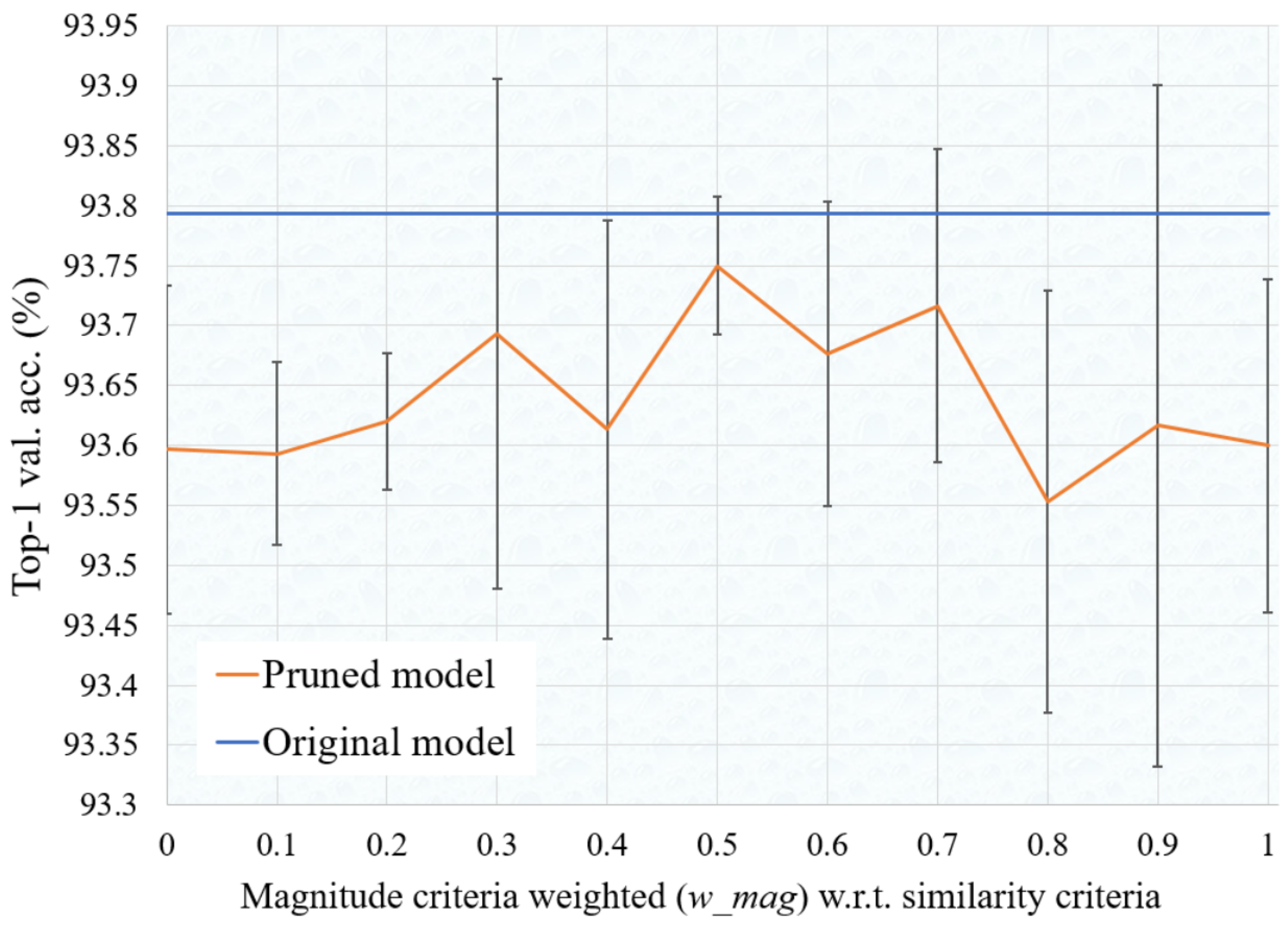
The proposed algorithm uses both magnitude and similarity criteria for filter selection during pruning. Therefore it is required to pass the parameter defining the pruning ratio for magnitude-based pruning and similarity-based pruning to match the final pruning ratio. This is defined by $w_{mag}$ parameter which ranges from 0 to 1. If we set $w_{mag}$ to 0, only similarity-based criteria is used for filter selection. Similarly, if we set $w_{mag}$ to 1, only magnitude criteria is used for filter selection. We experiment with different values of $w_{mag}$ for VGGNet pruning on the CIFAR-10 dataset, which is show in Figure 1. It is found that setting $w_{mag}$ value around $0.5$ produce the best results. Therefore, for all experiments in this paper, we set $w_{mag}$ to $0.5$, which means we set equal weight for magnitude criteria and similarity criteria.

4.5.2. Analysis of Pruning and Fine-Tuning

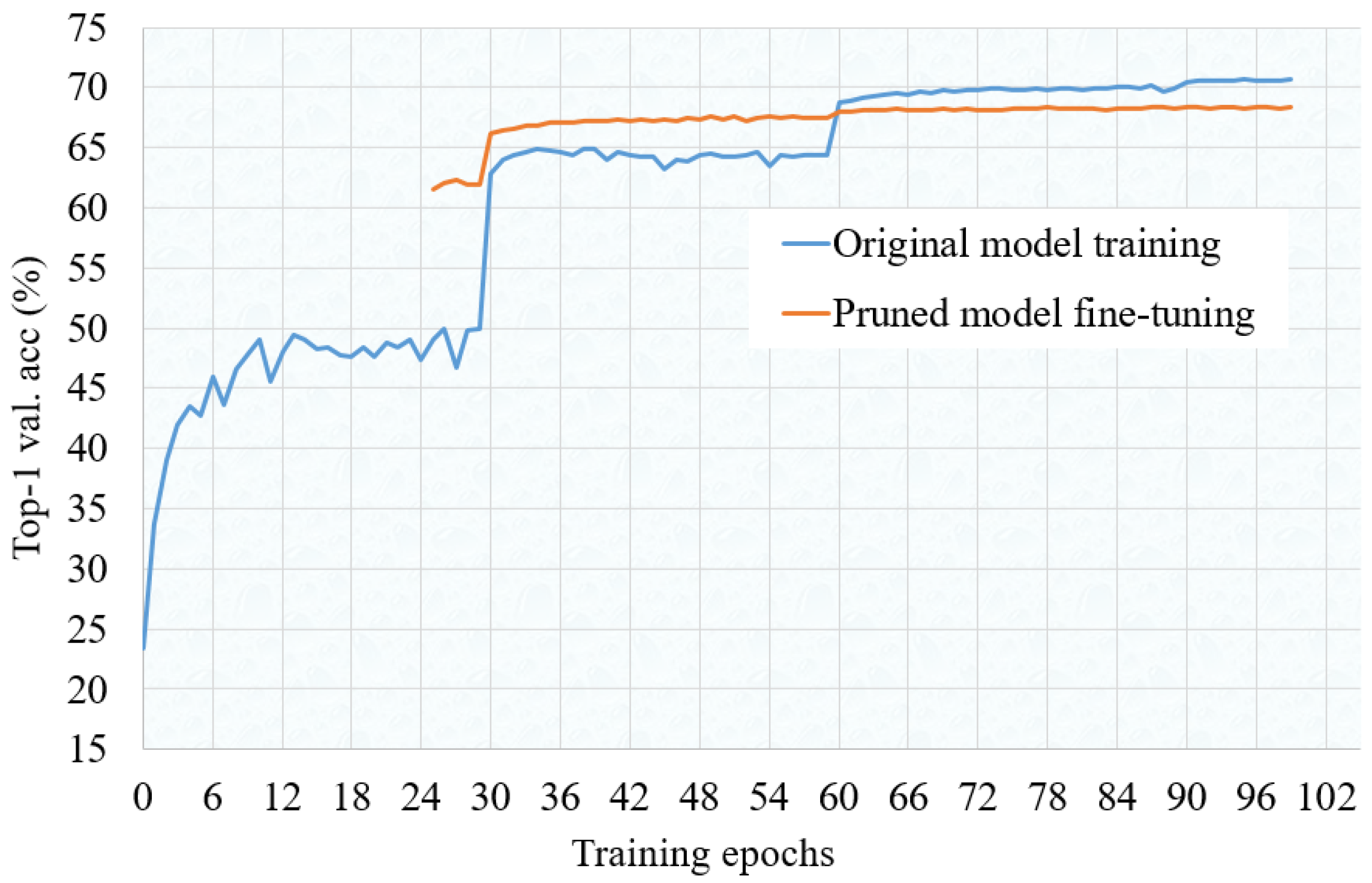
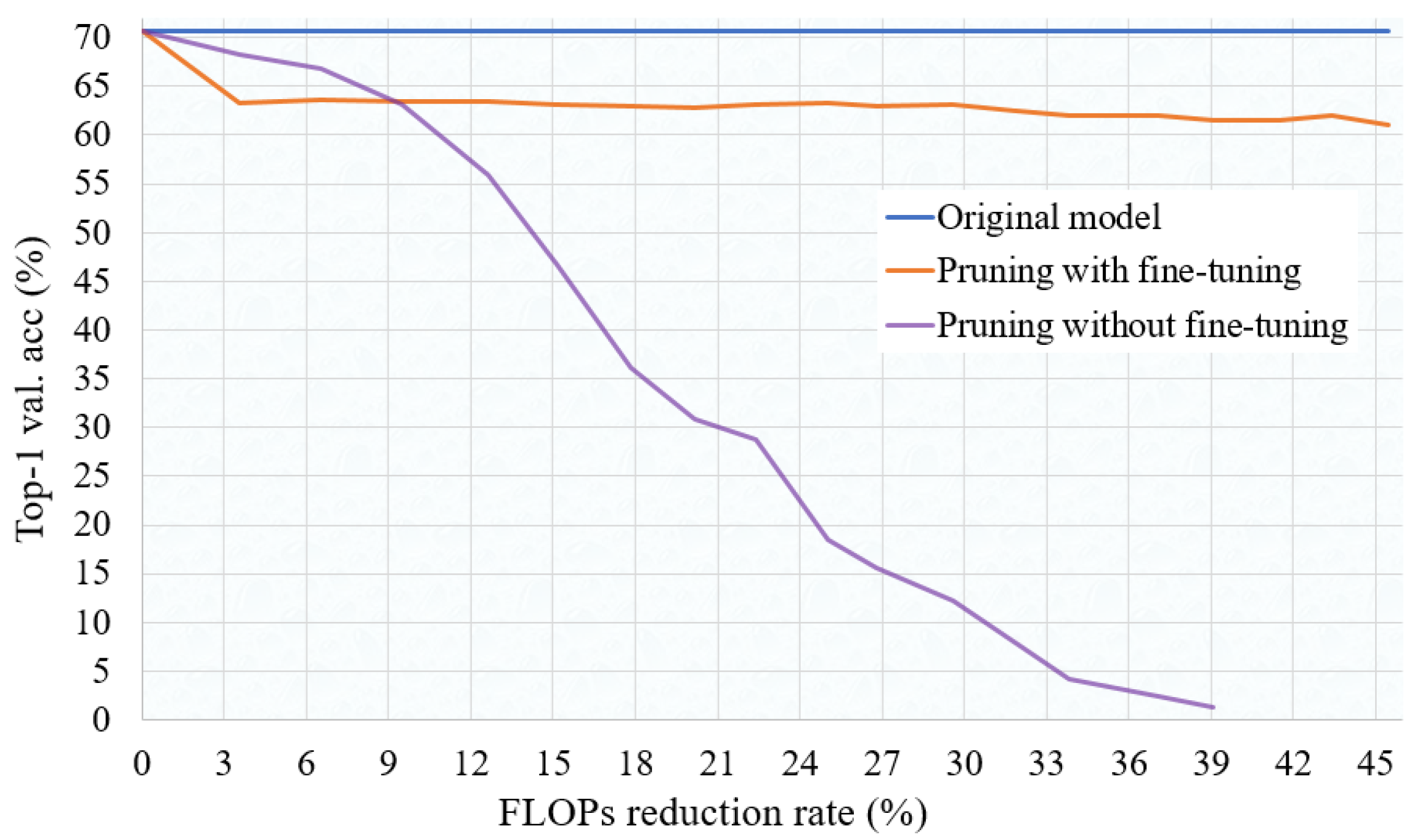
We analyze the pruning and fine-tuning process in detail for the ResNet-18 model using the ImageNet dataset. Figure 2 shows the validation accuracy across 0 to 100 training epochs. Once the baseline training is completed, as shown in Figure 3, iterative pruning is carried out to achieve desired FLOPs reduction rate. In order to maintain the validation accuracy, fine-tuning is performed at least for one training epoch after every 3% FLOPs reduction rate, which is obtained empirically. The starting learning rate for fine-tuning is set to 10% of the original learning rate. From Figure 3 we can see that after the first 3% FLOPs reduction, and after fine-tuning, the validation accuracy drops from 70.65% to 63.26%. This drop is obvious because also in Figure 2 we see that at the same learning rate, the original network accuracy is also around 64%. During pruning, the accuracy maintains above 61% achieving a 54% FLOPs reduction rate, and finally reaches 68.43% after completion of the final fine-tuning. Figure 3 also shows how abruptly accuracy drops if fine-tuning is not performed during pruning. That means in Algorithm 1, if we skip Lines 22∼25, accuracy drops to almost 1% as soon as we reach FLOPs reduction rate to 40%. As shown in Figure 2, we start final fine-tuning from 25th epoch, because during pruning we also run fine-tuning at least 15 times. Therefore it is not necessary to start fine-tuning from 0th epoch. Also, it is seen that pruned model converges in the early epoch and fine-tuning is not required until the 100th epoch. Therefore, a much less number of training epochs are required for fine-tuning the slimmed model compared to the baseline training.

5. Conclusions and Future Work

In this paper, we propose a simple yet effective variable rate filter pruning method for deep CNN acceleration, named MSVFP. The proposed method utilizes both magnitude and similarity-based filter selection criteria while preventing abrupt accuracy loss during pruning. The optimal set of filters in terms of model overall loss is selected and pruned from the specific layer of the network until the target pruning rate is achieved. The pruning algorithm is designed in such a way that in every pruning iteration pruning CNN layer and the set of filters to be pruned are automatically selected. Consequently, instead of fixed rate pruning, at the end of the pruning process, filters from each layer with different pruning rates are removed. The pruning results on the small and large-scale benchmark datasets with different CNN architectures show that MSVFP advances several popular state-of-the-art methods. In the case of VGG-16 pruning on the CIFAR-10 dataset, even after pruning more than $50\%$ of the network FLOPs, there is no accuracy drop. Again, while pruning ResNet-56 and ResNet-110 on the CIFAR-10 dataset with more than $52\%$ FLOPs reduction rate, the top-1 accuracy of the pruned model even advances by $0.11\%$ and $0.23\%$, respectively. Also, while pruning the ResNet-50 model on the ImageNet benchmark dataset with more than $53\%$ FLOPs reduction rate, there is only $1.11\%$ top-1 and $0.55\%$ top-5 accuracy drop w.r.t. baseline accuracy.

In the future, we will focus on replacing the traditional train-prune-retrain method used in this paper with a more advanced pruning-while-training technique utilizing a similar filter selection strategy. Again, although we tried to minimize computation cost using a small subset of the training dataset for loss estimation due to pruning, it will be better to completely remove the involvement of the training dataset during the pruning process. In the proposed algorithm we manually partition the whole filter selection criteria among the magnitude criteria and similarity criteria. In future work, instead of manual partitioning, we may also consider the automatic selection of optimal filter selection criteria from the pool of available criteria, as different layers have various peculiarities and the distribution of filters across layers and networks with various benchmark datasets is also different. Moreover, it will be interesting to see the effectiveness of the proposed method on more advanced CNN applications such as object detection, image segmentation, face recognition, etc.

References

- Xiao, L.; Bahri, Y.; Sohl-Dickstein, J.; Schoenholz, S.; Pennington, J. Dynamical isometry and a mean field theory of cnns: How to train 10,000-layer vanilla convolutional neural networks. In Proceedings of the International Conference on Machine Learning, PMLR, Stockholm, Sweden, 10–15 July 2018; pp. 5393–5402. [Google Scholar]
- Bianco, S.; Cadene, R.; Celona, L.; Napoletano, P. Benchmark analysis of representative deep neural network architectures. IEEE Access 2018, 6, 64270–64277. [Google Scholar] [CrossRef]
- Russakovsky, O.; Deng, J.; Su, H.; Krause, J.; Satheesh, S.; Ma, S.; Huang, Z.; Karpathy, A.; Khosla, A.; Bernstein, M.; et al. Imagenet large scale visual recognition challenge. Int. J. Comput. Vis. 2015, 115, 211–252. [Google Scholar] [CrossRef] [Green Version]
- Tan, M.; Chen, B.; Pang, R.; Vasudevan, V.; Sandler, M.; Howard, A.; Le, Q.V. Mnasnet: Platform-aware neural architecture search for mobile. In Proceedings of the IEEE/CVF Conference on Computer Vision and Pattern Recognition, Long Beach, CA, USA, 16–20 June 2019; pp. 2820–2828. [Google Scholar]
- Zhang, M.; Li, H.; Pan, S.; Chang, X.; Zhou, C.; Ge, Z.; Su, S. One-shot neural architecture search: Maximising diversity to overcome catastrophic forgetting. IEEE Trans. Pattern Anal. Mach. Intell. 2020, 43, 2921–2935. [Google Scholar] [CrossRef] [PubMed]
- Chen, Y.H.; Krishna, T.; Emer, J.S.; Sze, V. Eyeriss: An energy-efficient reconfigurable accelerator for deep convolutional neural networks. IEEE J. Solid-State Circuits 2016, 52, 127–138. [Google Scholar] [CrossRef] [Green Version]
- Zhang, S.; Du, Z.; Zhang, L.; Lan, H.; Liu, S.; Li, L.; Guo, Q.; Chen, T.; Chen, Y. Cambricon-X: An accelerator for sparse neural networks. In Proceedings of the 49th Annual IEEE/ACM International Symposium on Microarchitecture (MICRO), Taipei, Taiwan, 15–19 October 2016; pp. 1–12. [Google Scholar]
- Deng, L.; Li, G.; Han, S.; Shi, L.; Xie, Y. Model compression and hardware acceleration for neural networks: A comprehensive survey. Proc. IEEE 2020, 108, 485–532. [Google Scholar] [CrossRef]
- Ghimire, D.; Kil, D.; Kim, S.h. A Survey on Efficient Convolutional Neural Networks and Hardware Acceleration. Electronics 2022, 11, 945. [Google Scholar] [CrossRef]
- Han, S.; Mao, H.; Dally, W.J. Deep compression: Compressing deep neural networks with pruning, trained quantization and huffman coding. arXiv 2015, arXiv:1510.00149. [Google Scholar]
- Frankle, J.; Carbin, M. The lottery ticket hypothesis: Finding sparse, trainable neural networks. arXiv 2018, arXiv:1803.03635. [Google Scholar]
- Ding, X.; Zhou, X.; Guo, Y.; Han, J.; Liu, J. Global sparse momentum sgd for pruning very deep neural networks. Adv. Neural Inf. Process. Syst. 2019, 32, 6382–6394. [Google Scholar]
- He, Y.; Kang, G.; Dong, X.; Fu, Y.; Yang, Y. Soft filter pruning for accelerating deep convolutional neural networks. arXiv 2018, arXiv:1808.06866. [Google Scholar]
- He, Y.; Ding, Y.; Liu, P.; Zhu, L.; Zhang, H.; Yang, Y. Learning filter pruning criteria for deep convolutional neural networks acceleration. In Proceedings of the IEEE/CVF Conference on Computer Vision and Pattern Recognition, Virtual, 14–19 June 2020; pp. 2009–2018. [Google Scholar]
- He, Y.; Liu, P.; Wang, Z.; Hu, Z.; Yang, Y. Filter pruning via geometric median for deep convolutional neural networks acceleration. In Proceedings of the IEEE/CVF Conference on Computer Vision and Pattern Recognition, Long Beach, CA, USA, 16–20 June 2019; pp. 4340–4349. [Google Scholar]
- He, Y.; Liu, P.; Zhu, L.; Yang, Y. Filter pruning by switching to neighboring CNNs with good attributes. IEEE Trans. Neural Netw. Learn. Syst. 2022, 1–13. [Google Scholar] [CrossRef] [PubMed]
- Jung, S.; Son, C.; Lee, S.; Son, J.; Han, J.J.; Kwak, Y.; Hwang, S.J.; Choi, C. Learning to quantize deep networks by optimizing quantization intervals with task loss. In Proceedings of the IEEE/CVF Conference on Computer Vision and Pattern Recognition, Long Beach, CA, USA, 16–20 June 2019; pp. 4350–4359. [Google Scholar]
- Banner, R.; Nahshan, Y.; Soudry, D. Post training 4-bit quantization of convolutional networks for rapid-deployment. Adv. Neural Inf. Process. Syst. 2019, 32, 7950–7958. [Google Scholar]
- Jacob, B.; Kligys, S.; Chen, B.; Zhu, M.; Tang, M.; Howard, A.; Adam, H.; Kalenichenko, D. Quantization and training of neural networks for efficient integer-arithmetic-only inference. In Proceedings of the IEEE Conference on Computer Vision and Pattern Recognition, Salt Lake City, UT, USA, 18–23 June 2018; pp. 2704–2713. [Google Scholar]
- Polino, A.; Pascanu, R.; Alistarh, D. Model compression via distillation and quantization. arXiv 2018, arXiv:1802.05668. [Google Scholar]
- Ji, M.; Shin, S.; Hwang, S.; Park, G.; Moon, I.C. Refine myself by teaching myself: Feature refinement via self-knowledge distillation. In Proceedings of the IEEE/CVF Conference on Computer Vision and Pattern Recognition, Virtual, 19–25 June 2021; pp. 10664–10673. [Google Scholar]
- Yang, H.; Tang, M.; Wen, W.; Yan, F.; Hu, D.; Li, A.; Li, H.; Chen, Y. Learning low-rank deep neural networks via singular vector orthogonality regularization and singular value sparsification. In Proceedings of the IEEE/CVF Conference on Computer Vision and Pattern Recognition Workshops, Virtual, 14–19 June 2020; pp. 678–679. [Google Scholar]
- Yin, M.; Sui, Y.; Liao, S.; Yuan, B. Towards efficient tensor decomposition-based dnn model compression with optimization framework. In Proceedings of the IEEE/CVF Conference on Computer Vision and Pattern Recognition, Virtual, 19–25 June 2021; pp. 10674–10683. [Google Scholar]
- Li, H.; Kadav, A.; Durdanovic, I.; Samet, H.; Graf, H.P. Pruning filters for efficient convnets. arXiv 2016, arXiv:1608.08710. [Google Scholar]
- Mondal, M.; Das, B.; Roy, S.D.; Singh, P.; Lall, B.; Joshi, S.D. Adaptive CNN filter pruning using global importance metric. Comput. Vis. Image Underst. 2022, 222, 103511. [Google Scholar] [CrossRef]
- Luo, J.H.; Wu, J.; Lin, W. Thinet: A filter level pruning method for deep neural network compression. In Proceedings of the IEEE International Conference on Computer Vision, Venice, Italy, 22–29 October 2017; pp. 5058–5066. [Google Scholar]
- Yu, R.; Li, A.; Chen, C.F.; Lai, J.H.; Morariu, V.I.; Han, X.; Gao, M.; Lin, C.Y.; Davis, L.S. Nisp: Pruning networks using neuron importance score propagation. In Proceedings of the IEEE Conference on Computer Vision and Pattern Recognition, Salt Lake City, UT, USA, 18–23 June 2018; pp. 9194–9203. [Google Scholar]
- Han, S.; Pool, J.; Tran, J.; Dally, W. Learning both weights and connections for efficient neural network. Adv. Neural Inf. Process. Syst. 2015, 28, 1135–1143. [Google Scholar]
- Kim, T.; Choi, H.; Choe, Y. Automated Filter Pruning Based on High-Dimensional Bayesian Optimization. IEEE Access 2022, 10, 22547–22555. [Google Scholar] [CrossRef]
- Lin, M.; Zhang, Y.; Li, Y.; Chen, B.; Chao, F.; Wang, M.; Li, S.; Tian, Y.; Ji, R. 1xn pattern for pruning convolutional neural networks. IEEE Trans. Pattern Anal. Mach. Intell. 2022, 1–11. [Google Scholar] [CrossRef]
- Wang, T.; Wang, K.; Cai, H.; Lin, J.; Liu, Z.; Wang, H.; Lin, Y.; Han, S. Apq: Joint search for network architecture, pruning and quantization policy. In Proceedings of the IEEE/CVF Conference on Computer Vision and Pattern Recognition, Virtual, 14–19 June 2020; pp. 2078–2087. [Google Scholar]
- Blalock, D.; Gonzalez Ortiz, J.J.; Frankle, J.; Guttag, J. What is the state of neural network pruning? Proc. Mach. Learn. Syst. 2020, 2, 129–146. [Google Scholar]
- LeCun, Y.; Denker, J.; Solla, S. Optimal brain damage. Adv. Neural Inf. Process. Syst. 1989, 2, 598–605. [Google Scholar]
- Alabdulmohsin, I.; Markeeva, L.; Keysers, D.; Tolstikhin, I. A generalized lottery ticket hypothesis. arXiv 2021, arXiv:2107.06825. [Google Scholar]
- Bai, Y.; Wang, H.; TAO, Z.; Li, K.; Fu, Y. Dual Lottery Ticket Hypothesis. In Proceedings of the International Conference on Learning Representations, Virtual, 22–25 April 2022. [Google Scholar]
- Aghasi, A.; Abdi, A.; Nguyen, N.; Romberg, J. Net-trim: Convex pruning of deep neural networks with performance guarantee. Adv. Neural Inf. Process. Syst. 2017, 30, 3180–3189. [Google Scholar]
- Chin, T.W.; Ding, R.; Zhang, C.; Marculescu, D. Towards efficient model compression via learned global ranking. In Proceedings of the IEEE/CVF Conference on Computer Vision and Pattern Recognition, Seattle, WA, USA, 14–19 June 2020; pp. 1518–1528. [Google Scholar]
- Lin, M.; Cao, L.; Li, S.; Ye, Q.; Tian, Y.; Liu, J.; Tian, Q.; Ji, R. Filter sketch for network pruning. IEEE Trans. Neural Netw. Learn. Syst. 2021, 33, 7091–7100. [Google Scholar] [CrossRef] [PubMed]
- Krizhevsky, A.; Hinton, G. Learning Multiple Layers of Features from Tiny Images; Technical Report; University of Toronto: Toronto, ON, Canada, 2009. [Google Scholar]
- He, K.; Zhang, X.; Ren, S.; Sun, J. Deep residual learning for image recognition. In Proceedings of the IEEE Conference on Computer Vision and Pattern Recognition, Las Vegas, NV, USA, 27–30 June 2016; pp. 770–778. [Google Scholar]
- Simonyan, K.; Zisserman, A. Very deep convolutional networks for large-scale image recognition. arXiv 2014, arXiv:1409.1556. [Google Scholar]
- He, K.; Zhang, X.; Ren, S.; Sun, J. Identity mappings in deep residual networks. In European Conference on Computer Vision; Springer: Berlin/Heidelberg, Germany, 2016; pp. 630–645. [Google Scholar]
- Zagoruyko, S.; Komodakis, N. Wide residual networks. arXiv 2016, arXiv:1605.07146. [Google Scholar]
- Paszke, A.; Gross, S.; Chintala, S.; Chanan, G.; Yang, E.; DeVito, Z.; Lin, Z.; Desmaison, A.; Antiga, L.; Lerer, A. Automatic Differentiation in Pytorch. In Proceedings of the 31st Conference on Neural Information Processing Systems (NIPS), Long Beach, CA, USA, 4–9 December 2017. [Google Scholar]
- Fang, G. Torch-Pruning. Available online: https://github.com/VainF/Torch-Pruning (accessed on 20 December 2022).
- Joo, D.; Baek, S.; Kim, J. Which Metrics for Network Pruning: Final Accuracy? Or Accuracy Drop? In Proceedings of the 2022 IEEE International Conference on Image Processing (ICIP), Bordeaux, France, 16–19 October 2022; pp. 1071–1075. [Google Scholar]
- Dong, X.; Huang, J.; Yang, Y.; Yan, S. More is less: A more complicated network with less inference complexity. In Proceedings of the IEEE Conference on Computer Vision and Pattern Recognition, Honolulu, HI, USA, 21–26 July 2017; pp. 5840–5848. [Google Scholar]
- Lin, M.; Ji, R.; Wang, Y.; Zhang, Y.; Zhang, B.; Tian, Y.; Shao, L. Hrank: Filter pruning using high-rank feature map. In Proceedings of the IEEE/CVF Conference on Computer Vision and Pattern Recognition, Virtual, 14–19 June 2020; pp. 1529–1538. [Google Scholar]
- Gao, S.; Huang, F.; Cai, W.; Huang, H. Network pruning via performance maximization. In Proceedings of the IEEE/CVF Conference on Computer Vision and Pattern Recognition, Virtual, 19–25 June 2021; pp. 9270–9280. [Google Scholar]
- Liu, Z.; Sun, M.; Zhou, T.; Huang, G.; Darrell, T. Rethinking the value of network pruning. arXiv 2018, arXiv:1810.05270. [Google Scholar]
- Liu, Z.; Mu, H.; Zhang, X.; Guo, Z.; Yang, X.; Cheng, K.T.; Sun, J. Metapruning: Meta learning for automatic neural network channel pruning. In Proceedings of the IEEE/CVF International Conference on Computer Vision, Seoul, Republic of Korea, 27 October–2 November 2019; pp. 3296–3305. [Google Scholar]
- Singh, P.; Verma, V.K.; Rai, P.; Namboodiri, V. Leveraging filter correlations for deep model compression. In Proceedings of the IEEE/CVF Winter Conference on Applications of Computer Vision, Snowmass Village, CO, USA, 1–5 March 2020; pp. 835–844. [Google Scholar]
- Li, G.; Ma, X.; Wang, X.; Liu, L.; Xue, J.; Feng, X. Fusion-catalyzed pruning for optimizing deep learning on intelligent edge devices. IEEE Trans. Comput.-Aided Des. Integr. Circuits Syst. 2020, 39, 3614–3626. [Google Scholar] [CrossRef]
Figure 1.
VGGNet validation accuracy across various values of on the CIFAR-10 dataset.
Figure 2.
Validation accuracy across training epochs while baseline training and fine-tuning the pruned ResNet-18 model on the ImageNet dataset.
Figure 3.
Validation accuracy while pruning the baseline ResNet-18 model on the ImageNet dataset across different FLOPs reduction rates. After every 3% FLOPs reduction, fine-tuning is performed for one epoch to prevent the accuracy drop.