IDEINFO: An Improved Vector-Weighted Optimization Algorithm

Abstract

This study proposes an improved vector-weighted averaging algorithm (IDEINFO) for the optimization of different problems. The original vector-weighted optimization algorithm (INFO) uses weighted averaging for entity structures and uses three core procedures to update the positions of the vectors. First, the update rule phase is based on the law of averaging and convergence acceleration to generate new vectors. Second, the vector combination phase combines the obtained vectors with the update rules to achieve a promising solution. Third, the local search phase helps the algorithm eliminate low-precision solutions and improve exploitability and convergence. However, this approach pseudo-randomly initializes candidate solutions, and therefore risks falling into local optima. We, therefore, optimize the initial distribution uniformity of potential solutions by using a two-stage backward learning strategy to initialize the candidate solutions, and a difference evolution strategy to perturb these vectors in the combination stage to produce improved candidate solutions. In the search phase, the search range of the algorithm is expanded according to the probability values combined with the t-distribution strategy, to improve the global search results. The IDEINFO algorithm is, therefore, a promising tool for optimal design based on the considerable efficiency of the algorithm in the case of optimization constraints.

1. Introduction

As society develops, so will the complexity of its problems. Solving these increasingly complex problems is a key part of promoting ongoing development. Traditional algorithms no longer meet the necessary performance requirements for such problems. However, extensive research on intelligent algorithms has led to successful industrial applications within the engineering domain, where global optimization of nonlinear and complex objective functions is particularly difficult. Metaheuristic algorithms provide the simplicity needed to solve complex path planning [1,2], engineering optimization [3,4], medical diagnosis [5], intelligent control [6], image engineering [7], and network structure optimization problems [8].

Although many traditional numerical analysis methods have been studied in this regard, some deterministic methods are still not fit to solve challenging problems in the field of highly nonlinear search, due to their complexity. The optimization of problems through the application of deterministic methods, such as Lagrangian or simplex methods, requires both initial information about the problem and complex computations. Therefore, it is not always possible or feasible to use such methods, for problems of this level, to explore the global optimal solution problem, and hence, there remains an urgent need to develop an effective method to solve increasingly complex optimization problems. In fact, optimization methods can take various forms and formulations, perhaps without the formal restrictions they necessitate for core development in stochastic class exploration. Problems dealing with these forms, such as multi-objective optimization, fuzzy optimization, robust optimization, modulo optimization, large-scale optimization, and single-objective optimization, can therefore be utilized.

In recent years, several population-based optimization algorithms have been applied as simple and reliable methods to solve problems in computer science and industry. Many researchers have demonstrated that these population-based approaches are promising for solving many challenging problems. Some algorithms use methods that mimic natural evolutionary mechanisms and basic genetic rules such as selection, reproduction, mutation, and migration [9]. One of the most popular evolutionary methods is the introduced genetic algorithm (GA) [10]. With their unique three core operations of crossover, mutation, and selection, genetic algorithms have achieved excellent performance on many optimization problems. Other popular evolutionary algorithms include differential evolution (DE) [11] and genetic programming (GP) [12]. Such evolutionary algorithms simulate the way organisms evolve in nature and are highly adaptable to optimization problems. Moreover, some methods are developed from the laws of physics, such as the simulated annealing algorithm (SA) [13], which simulates the annealing mechanism in physical materials science. Moreover, with its excellent local search capability, SA is used to optimize nonlinear and linearized problems such as multilayer perceptron (MLP) training for motor speed regulation, and proportional-integral differential controller design [14]. The Grey Wolf Optimization (GWO) algorithm [15,16] is a new population intelligence optimization algorithm widely used in many important fields. It primarily mimics the stratification pattern and hunting behavior of gray wolf packs, and optimizes through wolf stalking, encircling, and pouncing behaviors. Compared with traditional optimization algorithms such as PSO and GA, GWO has the advantages of fewer parameters, simple principles, and easy implementation. However, GWO also has disadvantages, such as a slow convergence speed, low solution accuracy, and easily falling into local optimality. One of the latest mature methods is the gradient-based optimizer (GBO) [17], which considers Newtonian logic to explore suitable regions and achieve a global solution. This method has been applied in many fields, including sentiment recognition [18] and parameter evaluation [19]. Most population approaches model the particle swarm optimization (PSO) equation by changing the heuristic basis of collective social behavior around a population of animals [20]. Particle Swarm Optimization (PSO) is one of the most successful algorithms of this type, inspired by the individual and collective intelligence of birds when they flock together. Specifically, PSO has some parameters that need to be adjusted and, unlike other methods, PSO has a memory machine that retains the knowledge of the better performing particles, which helps the algorithm to find the optimal solution faster. Currently, PSO has been engaged with the large-scale optimization problem. In addition, there are many newly developed improved intelligent optimization algorithms, for example, ref. [21] proposed an improved GWO to solve the instability and convergence accuracy problems when GWO is applied to mobile robot path planning as a metaheuristic algorithm with a powerful optimization search capability. In [22], an improved crawler search algorithm (IRSA), based on the sine cosine algorithm and Levy flight, was proposed. The improved sine cosine algorithm has an enhanced global search capability, avoids local minima traps by a comprehensive search of the solution space, and the Levy flight operator, with a jump size control factor, improves the exploitation capability of the search agent. A new metaheuristic optimization algorithm based on ancient warfare strategies was proposed in [23], introducing a new weight update mechanism and a weak troop migration strategy. The proposed warfare strategy algorithm achieves a good balance between the exploration and development phases.

Although the abovementioned optimization methods can solve a variety of challenging practical engineering optimization problems, according to the No Free Lunch (NFL) theorem [24], no single optimization method can be the best tool to solve all problems. The case where some form of structure exists over the set of objective values, rather than the typical total ordering. It is shown that in such cases, when attention is restricted to natural measures of performance and optimization algorithms that measure performance and optimize based on such structure, the “no free lunch” result holds for any class of problems with closed structure under permutations [25]. In contrast, the INFO algorithm, proposed in [26], is a forward-looking algorithm that provides a promising platform for the future of the optimization literature in computer science through innovative attempts to target this approach. Our goal is to apply this improved vector-weighted averaging method to various optimization problems and make it a scalable optimizer.

In [26], a new optimizer (INFO) is designed, that can form a more stable structure by modifying the weighted averaging and updating the position of the vectors. The update phase, the combination phase, and the local search are the three core steps of INFO. Unlike other methods, the mean-based update rule is used in INFO to generate new vectors, which will speed up the convergence. In the vector combination phase, the two vectors obtained in the vector update phase are combined to generate a new vector to improve the local search capability. This operation ensures the diversity of the population to some extent. Considering the global optimal position and the mean-based rule, the local operation can effectively improve the vulnerability of the information material to local optima. The focus introduces the three core procedures mentioned above to optimize various optimization cases and engineering problems, such as structural and mechanical engineering problems and water resource systems. The INFO algorithm uses the concept of weighted averages to move agents toward better positions. The main motivation for INFO is to emphasize its performance aspects, potentially solving some optimization problems that cannot be solved by other methods.

In general, evolutionary algorithms can be divided into two types: single-solution-based and population-based algorithms [27]. In the first case, the search process of the algorithm starts with a single solution and updates its position during the optimization process. The best-known single-solution-based algorithms include single-solution-based simulation algorithms, including simulated annealing (SA) [13]. However, their drawbacks are the plausibility of high positions captured in the local optimum and the failure of information exchange, as these methods have only a single trend in the opposite direction. GA, DE, PSO, Ant Colony Optimization (ACO) [28], Artificial Bee Colony (ABC) [29], Harris Hawkeye Optimization (HHO) [30], Hunger Games Search (HGS) [31], Rungakuta Optimizer (RUN) [32], Sticky Fungus Algorithm (SMA) [33], and Whale Optimization (WOA) [34] are some examples of population-based algorithms. These methods can eliminate local optimization because they use a set of solutions in the optimization process. In addition, information exchange can be shared between solutions, which helps them to search better in difficult search spaces. However, these algorithms require significant computational costs for function evaluation and high-dimensional computation during optimization. Based on the above discussion, population-based algorithms are considered more reliable and robust optimization methods than single-solution-based algorithms.

In general, the best formulation of the algorithm is investigated by evaluating different types of benchmark and engineering problems. Typically, the optimizer uses one or more operators to perform two phases: exploration and exploitation. An optimization algorithm requires a search mechanism to find promising regions in the search space, which is done in the exploration phase. The exploitation phase improves the local search capability and the speed of convergence to promising regions. Balancing these two phases is a challenging problem for any optimization algorithm. According to previous studies, no precise rules have been established so far to distinguish the most appropriate transition time from the exploration to the development phase, or the stochastic nature of this type of optimizer, due to its unexplored form [35]. Therefore, addressing this problem is crucial for developing and designing a stable and reliable optimization algorithm. Concerning the main challenges, in order to create a high-performance optimization algorithm, we focused on vector-weighted optimization algorithms with efficient optimization performance, which is based on the principle of vector-weighted averaging. By avoiding nature-inspired thinking, INFO can provide a promising way to avoid and reduce the challenges of other optimization algorithms, thus taking a step forward in having strong optimization capabilities for practical problems in the field of complex unknown search.

In this paper, we report on our improvements to the INFO algorithm, which provides the following contributions:

• A two-stage backward learning strategy that initializes candidate solutions, resulting in improved distribution uniformity and enhanced search capability.
• A DE strategy that perturbs vector individuals to iteratively generate candidate solutions via greedy selection, which eliminates poorly adapted vectors and improves the local search ability.
• A combined t-distribution and probabilistic strategy that expands the search range and avoids local optima traps.

To evaluate our algorithm’s performance, 14 sets of test functions are applied, improvement metrics are tested separately, and we compare our improved INFO model with the SSA, GWO, and baseline INFO algorithms.

2. Materials and Methods

2.1. INFO

INFO is a population-based optimizer that applies weighted averaging rules to vectors in a search space to find the optimal solution after several consecutive generations. The baseline model has the advantages of strong search optimization and fast convergence [26]. The following subsections describe the phases of the algorithm’s operation.

2.2. Initialization Phase

The INFO algorithm comprises a population of $D$ vectors in an $Np$-dimensional search domain. In this step, the algorithm applies two main control parameters: weighted average $\delta$ and proportionality $\sigma$. Generally, the scale factor is increased by updating the regular operator to obtain a vector, which depends on the size of the search domain. $\sigma$ is used to calculate the exponential weighted averages of vectors. These parameters do not require fine-tuning and are dynamically updated during generation.

2.3. Update-Rule Phase

The update-rule operation increases the diversity of the population during the search using the weighted average of vectors to create new vectors. This phase consists of two main activities. The first starts with a random initial solution and extracts the weighted mean of a set of random vectors to move to the next candidate solution. The second activity accelerates convergence. This process is defined by Equations (1)–(4).

If $rand$ < 0.5,

$$z{1}_l^g=x_l^g+\sigma \times MeanRule+randn\times \frac{\left(x_{bs}-x_{a1}^g\right)}{\left(f\left(x_{bs}\right)-f\left(x_{a1}^g\right)+1\right)},$$

(1)

$$2_l^g=x_{bs}+\sigma \times MeanRule+randn\times \frac{\left(x_{a1}^g-x_b^g\right)}{\left(f\left(x_{a1}^g\right)-f\left(x_{a2}^g\right)+1\right)};$$

(2)

otherwise,

$$z{1}_l^g=x_a^g+\sigma \times MeanRule+randn\times \frac{\left(x_{a2}^g-x_{a3}^g\right)}{\left(f\left(x_{a2}^g\right)-f\left(x_{a3}^g\right)+1\right)},$$

(3)

$$z{2}_l^g=x_{bt}+\sigma \times MeanRule+randn\times \frac{\left(x_{a1}^g-x_{a2}^g\right)}{\left(f\left(x_{a1}^g\right)-f\left(x_{a2}^g\right)+1\right)},$$

(4)

where $z{1}_l^g$ and $z{2}_l^g$ are the new position vectors for the gth iteration, $\sigma$ represents the scaling factor of vectors, and $\alpha 1\ne \alpha 2\ne \alpha 3\ne 1$. $\sigma$ and $\alpha$ are calculated using Equations (5) and (6), respectively, where $\alpha$ is a random integer in $\left[1,Np\right]$; $randn$ is a random value in a standard positive terrestrial distribution.

$$\sigma =2\alpha \times rand-\alpha ,$$

(5)

$$\alpha =2\times exp\left(-4\times \frac{g}{Maxg}\right),$$

(6)

$$MeanRule=r\times WM{1}_l^g+\left(1-r\right)\times WM{2}_l^g,$$

(7)

where $r$ is a random number in $\left[0, 0.5\right]$, and $l=1,2,\dots ,Np. WM{2}_l^g$ is defined as follows:

$$WM{2}_l^g=\delta \times \frac{w_1\left(x_{a1}-x_{a2}\right)+w_2\left(x_{a1}-x_{a3}\right)+w_3\left(x_{a2}-x_{a3}\right)}{w_1+w_2+w_3+\epsilon }+\epsilon \times rand.$$

(8)

For $WM{1}_l^g$,$l=1,2,\dots ,Np$, and its w₁, w₂, w₃, and $\omega$ are expressed as follows:

$$w_1=cos\left(\left(f\left(x_{a1}\right)-f\left(x_{a2}\right)\right)+\pi \right)\times exp\left(-\left|\frac{f\left(x_{a1}\right)-f\left(x_{a2}\right)}{\omega }\right|\right),$$

(9)

$$w_2=cos\left(\left(f\left(x_{a1}\right)-f\left(x_{a3}\right)\right)+\pi \right)\times exp\left(-\left|\frac{f\left(x_{a1}\right)-f\left(x_{a3}\right)}{\omega }\right|\right),$$

(10)

$$w_3=cos\left(\left(f\left(x_{a2}\right)-f\left(x_{a3}\right)\right)+\pi \right)\times exp\left(-\left|\frac{f\left(x_{a2}\right)-f\left(x_{a3}\right)}{\omega }\right|\right),$$

(11)

$$\omega =max\left(f\left(x_{a1}\right),f\left(x_{a2}\right),f\left(x_{a3}\right)\right),$$

(12)

$$M{2}_l^g=\delta \times \frac{w_1\left(x_{bs}-x_{bt}\right)+w_2\left(x_{bs}-x_{ws}\right)+w_3\left(x_{bt}-x_{ws}\right)}{w_1+w_2+w_3+\epsilon }+\epsilon \times rand.$$

(13)

For $WM{2}_l^g$,$l=1,2,\dots ,Np$, and its w₁, w₂, w₃, and $\omega$ are expressed as follows:

$$w_1=cos\left(\left(f\left(x_{bs}\right)-f\left(x_{bt}\right)\right)+\pi \right)\times exp\left(-\left|\frac{f\left(x_{bs}\right)-f\left(x_{bt}\right)}{\omega }\right|\right),$$

(14)

$$w_2=cos\left(\left(f\left(x_{bs}\right)-f\left(x_{ws}\right)\right)+\pi \right)\times exp\left(-\left|\frac{f\left(x_{bs}\right)-f\left(x_{ws}\right)}{\omega }\right|\right),$$

(15)

$$w_3=cos\left(\left(f\left(x_{bt}\right)-f\left(x_{ws}\right)\right)+\pi \right)\times exp\left(-\left|\frac{f\left(x_{bt}\right)-f\left(x_{ws}\right)}{\omega }\right|\right),$$

(16)

$$\omega =f\left(x_{ws}\right),$$

(17)

$$\delta =2\beta \times rand-\beta ,$$

(18)

$$\alpha =\beta =2exp\left(-4\times \frac{g}{Maxg}\right).$$

(19)

Weighting functions w₁, w₂, and w₃ are used to calculate the weighted averages of the vectors, and x_bs, x_bt, and x_ws are the optimal, suboptimal, and worst solution vectors in the first $g$ generations of the population, respectively.

Convergence acceleration (CA) is added to the update-rule operator to improve the global search capability and find the best vector in the search space. With the INFO algorithm, the best solution is assumed to be the one closest to the global optimum. Hence, CA moves the vector in that direction. The CA presented in the equation is multiplied by a random number in the range [0, 1] at each step, and new vectors are computed as follows:

$$CA=randn\times \frac{\left(x_{bs}-x_{a1}\right)}{\left(f\left(x_{bs}\right)-f\left(x_{a1}\right)+\epsilon \right)},$$

(20)

$$z_l^g=x_l^g+\delta \times MeanRule+CA.$$

(21)

2.4. Vector-Merging Stage

In this stage, INFO combines vectors $z{1}_l^g$ and $z{2}_l^g$ with $rand<0.5$ to generate the new vector, $u_1^g$.

If $rand1<0.5$ and $rand2<0.5$,

$$u_l^g=z{1}_l^g+\mu \left|z{1}_l^g-z{2}_l^g\right|;$$

(22)

otherwise, if $rand1<0.5$ and $rand2\ge 0.5$,

$$u_l^g=z{2}_l^g+\mu \left|z{1}_l^g-z{2}_l^g\right|.$$

(23)

In either case, when $rand1<0.5$,

$$u_l^g=x_l^g,$$

(24)

where $u_l^g$ is the new vector formed by combining the first $g$ generational vectors, and $\mu =0.05\times randn$.

2.5. Local Search Phase

The local search phase aims to avoid local optima and generate a new vector when $rand<0.5$.

$$xrnd=\varphi \times x_{avg}+\left(1-\varphi \right)\times \left(\varphi \times x_{bt}+\left(1-\varphi \right)\times x_{bs}\right),$$

(25)

$$x_{avg}=\frac{\left(xa+xb+x3\right)}{3},$$

(26)

If $rand1<0.5$ and $rand2<0.5$,

$$u_1^g=xbs+randn\times \left(MeanRule+randn\times \left(x_{bs}^g-x_{a1}^g\right)\right);$$

(27)

otherwise, if $rand1<0.5 \mathrm{a}$nd$rand2\ge 0.5$,

$$u_1^g=xrnd+randn\times \left(MeanRule+randn\times \left(v1\times x_{bs}-v2\times x_{rnd}\right)\right),$$

(28)

where $\varphi$ is a random value in $\left[0, 1\right]$, x_rnd is a new solution made by combining x_avg, x_bt, and x_bs, and v₁ and v₂ are two random numbers defined as follows:

$$v1=\{\begin{array}{c}2\times rand\\ 1\end{array}\begin{array}{c}p>0.5\\ p\le 0.5\end{array},$$

(29)

$$v2=\{\begin{array}{c}rand\\ 1\end{array}\begin{array}{c}p<0.5\\ p\ge 0.5\end{array}.$$

(30)

2.6. Improved INFO Algorithm Design

2.6.1. Two-Stage Backward Learning Strategy

Because the baseline INFO algorithm randomly initializes the positions of candidate solutions using pseudo-random numbers, local extrema traps are possible. Thus, it is expected that a reverse learning approach to initializing the population, combined with a greedy search, will improve the model’s global performance.

The reverse point learning model is defined as follows. Let the initial solution, $X\left(x_1,x_2,\dots ,x_d\right)$, be located at a point where $x_i\in \left[a_i,b_i\right], i\in \left[1,d\right]$. $a_i,b_i$ denotes the lower and upper limits of the ith dimensional coordinate, respectively, taking d as the dimension of the search space. The coordinates of the reverse point, $X_1\left({\stackrel{̑}{x}}_1,{\stackrel{̑}{x}}_2,\mathrm{...},{\stackrel{̑}{x}}_d\right)$, are then calculated as follows:

$${\stackrel{̑}{x}}_i=a_i+b_i-x_i.$$

(31)

The two-stage backward learning strategy is divided into random and basic backward learning types. The size of the random number in [0, 1] is compared to the switching probability (0.5) to select the backward learning stage. If P is less than this random number, basic backward learning is selected:

$$\overrightarrow{Cnew}=lbi+\left(ubi-\overrightarrow{C}\right);$$

(32)

otherwise, random reverse learning is applied:

$$\overrightarrow{Cnew}=lbi+R\left(ubi-\overrightarrow{C}\right).$$

(33)

$R$ is a random number in $\left(0,1\right)$, $lbi$ and $ubi$ are the upper and lower bounds, respectively, $\overrightarrow{C}$ denotes the position updated by concentration only, and $\overrightarrow{Cnew}$ denotes the new position obtained after the two learning stages.

Although this process accelerates convergence to a certain extent, there is no guarantee that the new solution will necessarily be better than the original. Hence, the greedy algorithm is applied for merit:

$$\overrightarrow{C}=\{\begin{array}{c}\overrightarrow{Cnew},f\left(\overrightarrow{Cnew}\right)\le f\left(\overrightarrow{C}\right)\\ \overrightarrow{C},f\left(\overrightarrow{Cnew}\right)>f\left(\overrightarrow{C}\right)\end{array}.$$

(34)

2.6.2. DE Strategy

To diversify the population, and expand the search range during each iteration, new child sparks are generated via the differential algorithm to potentially improve the vectors of the next generation [36,37]. DE performs vector synthesis with individuals to be mutated by randomly selecting three from the population and scaling their vector differences:

$$\{\begin{array}{c}{p}_i^{g+1}=x_{d1}^g+F\cdot \left(x_{d2}^g-x_{d3}^g\right)\\ i\ne d1\ne d2\ne d3\end{array},$$

(35)

where $x_{di}^g$ is the$g$th individual in the $di$th generation population, $F$ is the scaling factor that increases the operator with adaptive variation, and

$$F=F0\cdot 2^{\tau },$$

(36)

where$F0$ is the variation operator, which takes a value in $\left[0, 2\right]$, which is usually 0.5. $\tau =e^{1-\frac{Gm}{Gm-G}}$, $Gm$ is the maximum evolutionary generation, and $G$ is the current evolutionary generation. To increase the diversity of new populations, crossover operations are introduced as follows:

$$w_{i,j}^{g+1}=\{\begin{array}{c}{p}_{i,j}^{g+1},rand\left(0,1\right)\le R,or,j=jrand\\ x_{i,j}^g,other\end{array},$$

(37)

where$R\in \left[0, 1\right]$ is the crossover probability, $jrand$ is the random number, $p_{i,j}^{g+1}$ is the intermediate generated by the first $g$ generation population variation, $\left\{p_i^{g+1}|p_{i,j}^{mi{n}_{i,j}^{g+1}{}_{i,j}^{max}}\right\}$, and $x_{i,j}^g$ is the individual prior to variation. To determine whether $w_i^{g+1}$ can become an individual of the first $g+1$ generation populations, $p_i^{g+1}$ and $p_i^g$ are compared in terms of fitness, and the optimal value is selected as follows:

$$p_i^{g+1}=\{\begin{array}{c}{w}_i^{g+1},f\left(w_i^{g+1}\right)\le f\left(p_i^g\right)\\ p_i^g,other\end{array}.$$

(38)

2.6.3. t-Distribution Strategy with the Number of Iterations as a Parameter

The $T\left(n\right)$ distribution (i.e., student distribution) contains parametric degrees of freedom, $n$, which determine its curve shape. The smaller the value, the flatter the curve and lower the middle [38]. The $t-$ distribution algorithm perturbs the positions of the vectors to achieve population variation, as follows:

$$x_i^t=x_i+x_i\cdot t\left( iter \right),$$

(39)

where $x_i^t$ is the new position of the $i$th vector in the population after mutation, $x_i$ is the position of the individual before mutation, and $t\left(iter\right)$ is the value of the $t$-distribution using the number of iterations as the degrees of freedom.

In the early iterations, the value of $iter$ is small, and the results generated by the $t$-distribution are similar to the Coasean variant in economics, which has a strong global search capability. In later periods, the value of $iter$ grows, becoming more similar to the Gaussian variant, which has a strong local search capability. Thus, INFO’s algorithmic accuracy is improved.

2.6.4. Improving the INFO Algorithm with Refined Two-Stage Backward Learning DE and t-Distribution Strategies

The steps for improving the INFO algorithm based on two-stage backward learning DE and t-distribution strategies are presented as a flowchart in Figure 1. The stepwise descriptions are as follows:

Step 1: Initialize the algorithm parameters, including the population size, maximum number of iterations T, and variable dimensionality.

Step 2: The two-stage backward learning strategy initializes the vector positions and calculates the fitness of the individuals.

Step 3: Start iterations (t < T).

Step 4: Update the vector positions using the mean-value rule, calculate the average position of the population, and update the positions.

Step 5: Vector merging and position updating.

Step 6: Local searching and position updating.

Step 7: Calculate the current vector fitness and compare it to obtain the current optimal individual.

Step 8: Generate probability p and perturb the position of the vector using the DE strategy if p > 0.5, and vice versa, perturbing the position of the vector according to the t-distribution strategy.

Step 9: Calculate the vector fitness values after perturbation and compare and update the positions of the optimal vectors.

Step 10: The individual positions and fitness values of the best vectors are recorded.

Step 11: Repeat Steps 4–10, and when the maximum number of iterations is reached, the optimal vector position and fitness are output.

3. Results

3.1. Experimental Design and Test Functions

The performance evaluation in this article is based on an Intel(R) Core(TM) i5-4590 CPU, a 3.30 GHz main frequency, 8 GB of memory, and Windows 10 (64-bit)operating system. The programming software is MATLAB2022(a).

Table 1. Test function equations.

Function	Equation
F1	$F1\left(x\right)={\displaystyle {\displaystyle \sum }_{i=1}^n}\left|xi\right|+{\displaystyle {\displaystyle \prod }_{i=1}^n}\left|xi\right|$
F2	$F2\left(x\right)={\displaystyle {\displaystyle \sum }_{i=1}^n}{\left({\displaystyle {\displaystyle \sum }_{j=1}^i}xj\right)}^2$
F3	$F3\left(x\right)=max\left\{xi|1\le i\le n\right\}$
F4	$F4\left(x\right)={\displaystyle {\displaystyle \sum }_{i=1}^{n-1}}\left[100{(xi+1-x{i}^2)}^2+{(xi-1)}^2\right]$
F5	$F5\left(x\right)={\displaystyle {\displaystyle \sum }_{i=1}^n}{(\left[xi+0.5\right])}^2$
F6	$F6\left(x\right)={\displaystyle {\displaystyle \sum }_{i=1}^n}i{x}_i^4+random\left[0,1\right]$
F7	$F7\left(x\right)={\displaystyle {\displaystyle \sum }_{i=1}^n}-xisin(\sqrt{\left|xi\right|})$
F8	$F8\left(x\right)=-20exp(-0.2\sqrt{\frac{1}{n}{\displaystyle {\displaystyle \sum }_{i=1}^n}x{i}^2})-exp(\frac{1}{n}{\displaystyle {\displaystyle \sum }_{i=1}^n}cos(2\pi xi))+20+e$
F9	$F9\left(x\right)=\frac{\pi }{n}\left\{10sin(\pi y1)+{\displaystyle {\displaystyle \sum }_{i=1}}\left(yi-1{)}^2\left[1+10{sin}^2(\pi yi+1\right)\right]+{(yn-1)}^2\right\}$ $+{\displaystyle {\displaystyle \sum }_{i=1}^n}u\left(xi,10,100,4\right)yi=1+\frac{xi+1}{4}$ $u\left(xi,a,k,m\right)=\{\begin{array}{c}k{(xi-a)}^m\\ 0\\ k{(-xi-a)}^m\end{array}\begin{array}{c}xi>a\\ -a<xi<a\\ xi<-a\end{array}$
F10	$F10\left(x\right)=0.1\{{sin}^2(3\pi x1)+{\displaystyle {\displaystyle \sum }_{i=1}^n}\left(xi-1{)}^2\left[1+{sin}^2(3\pi xi+1\right)\right]$ $+\left(xn-1{)}^2\left[1+{sin}^2(2\pi xn\right)\right]\}+{\displaystyle {\displaystyle \sum }_{i=1}^n}u\left(xi,5,100,4\right)$
F11	$F11\left(x\right)={\displaystyle {\displaystyle \sum }_{i=1}^{11}}{\left[ai-\frac{x1\left(b{i}^2+bix2\right)}{b{i}^2+bix3+x4}\right]}^2$
F12	$F12\left(x\right)=4x{1}^2-2.1x{1}^4+\frac{1}{3}x{1}^6+x1x2-4x{2}^2+4x{2}^4$
F13	$F13\left(x\right)=-{\displaystyle {\displaystyle \sum }_{i=1}^7}{\left[\left(x-ai\right){(x-ai)}^T+ci\right]}^{-1}$
F14	$F14\left(x\right)=-{\displaystyle {\displaystyle \sum }_{i=1}^{10}}{\left[\left(x-ai\right){(x-ai)}^T+ci\right]}^{-1}$

lists the 14 benchmark functions, and

Table 2. Test function information.

Function	Dimensionality	Scope	Theoretical Minimum Value
F1	30	[−10, 10]	0
F2	30	[−100, 100]	0
F3	30	[−100, 100]	0
F4	30	[−30, 30]	0
F5	30	[−100, 100]	0
F6	30	[−1.28, 1.28]	0
F7	30	[−500, 500]	−12,569.5
F8	30	[−32, 32]	0
F9	30	[−50, 50]	0
F10	30	[−50, 50]	0
F11	4	[−5, 5]	0.1484
F12	2	[−5, 5]	−1
F13	4	[0, 10]	−1
F14	4	[0, 10]	−1

lists their dimensions, search ranges, and optimal objective function solutions. The parameter settings for each algorithm are given in

Table 3. Algorithm parameter setting.

Name of the Algorithm	Parameters	Max-Fes
GWO	$A\in \left[2,0\right]$	30,000
WOA	$a1\in \left[2,0\right],a2\in \left[-2,-1\right],b=1$	30,000
SSA	$c\in \left[2,0\right]$	30,000
INFO	$c=2,d=4$	30,000
INFO1	$c=2,d=4$	30,000
INFO2	$c=2,d=4$	30,000
IDEINFO	$c=2,d=4$	30,000

. For a fair comparison, the population size of all algorithms was set to 30, the maximum number of iterations was 1000, and each group of experiments was repeated 50 times to determine the final results [39].

3.2. Experimental Results

3.2.1. High-Dimensional Single-Objective Test Function

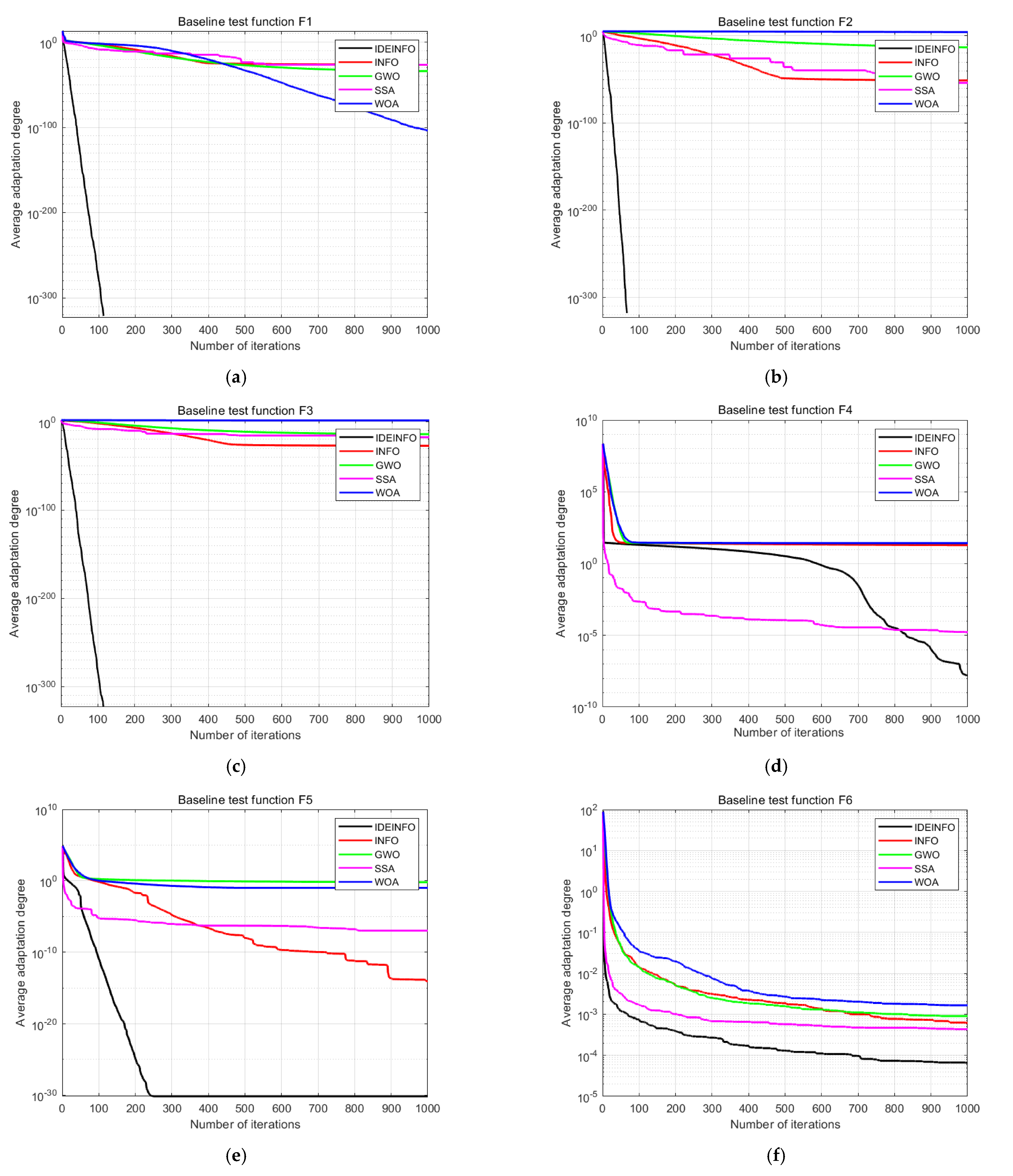
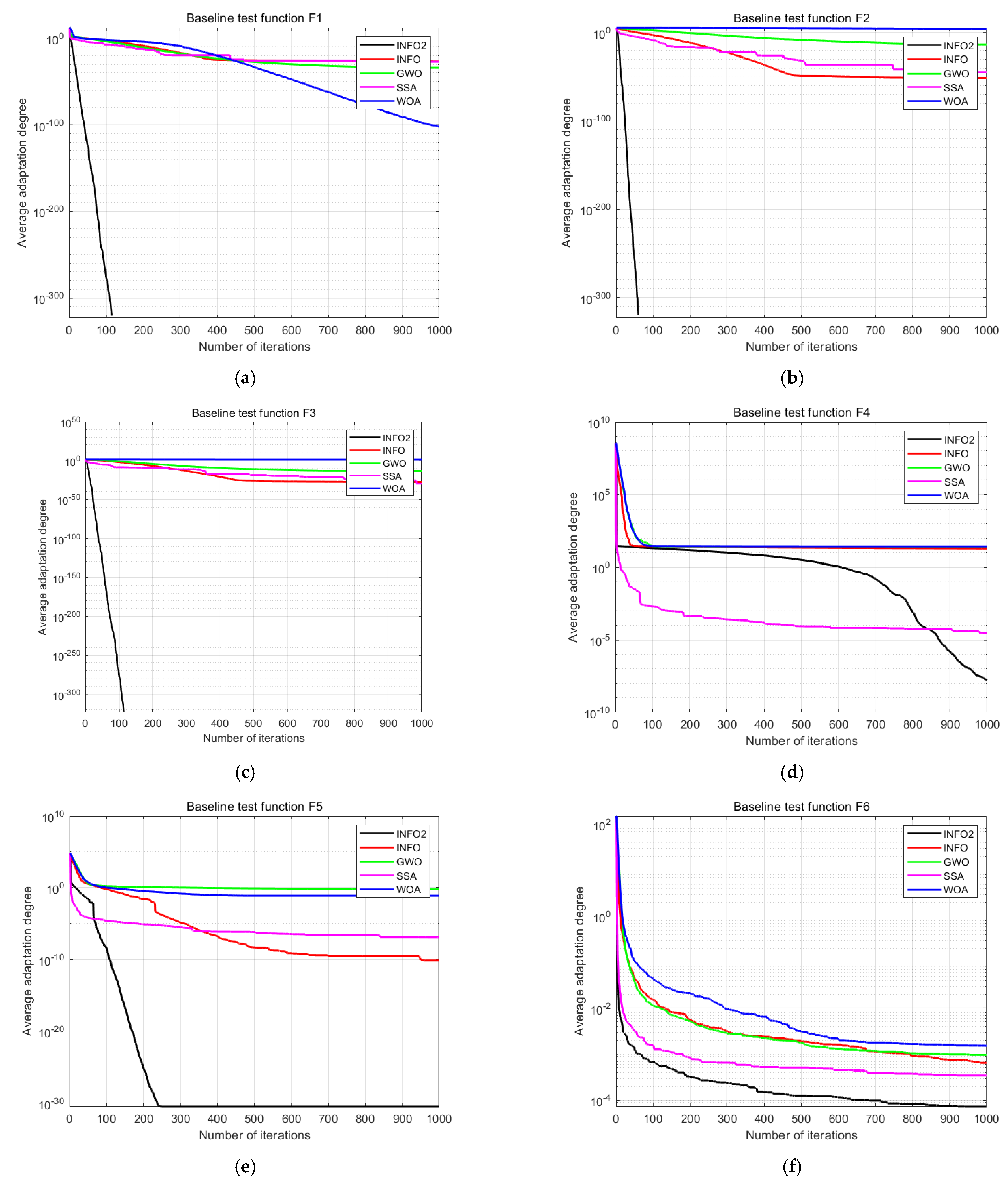
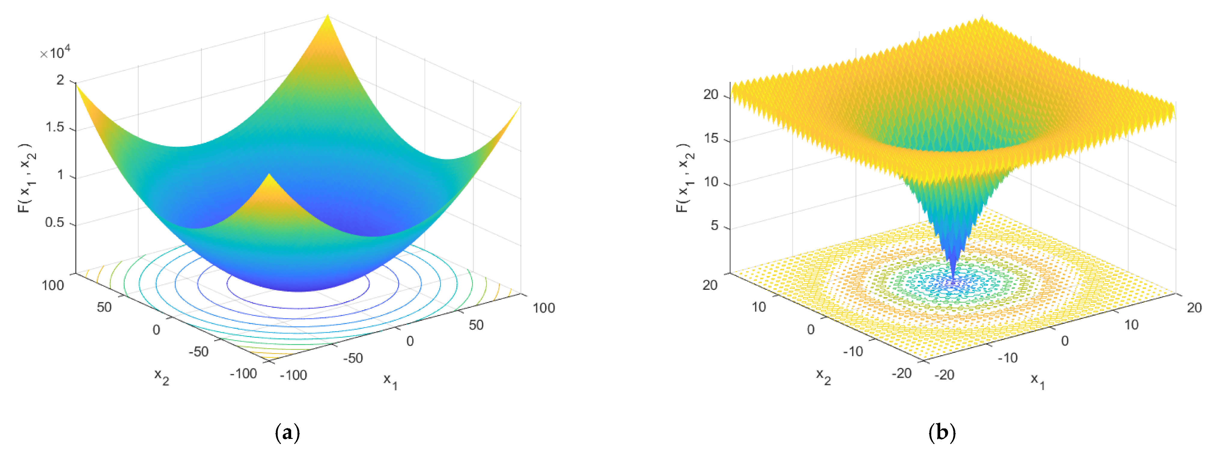
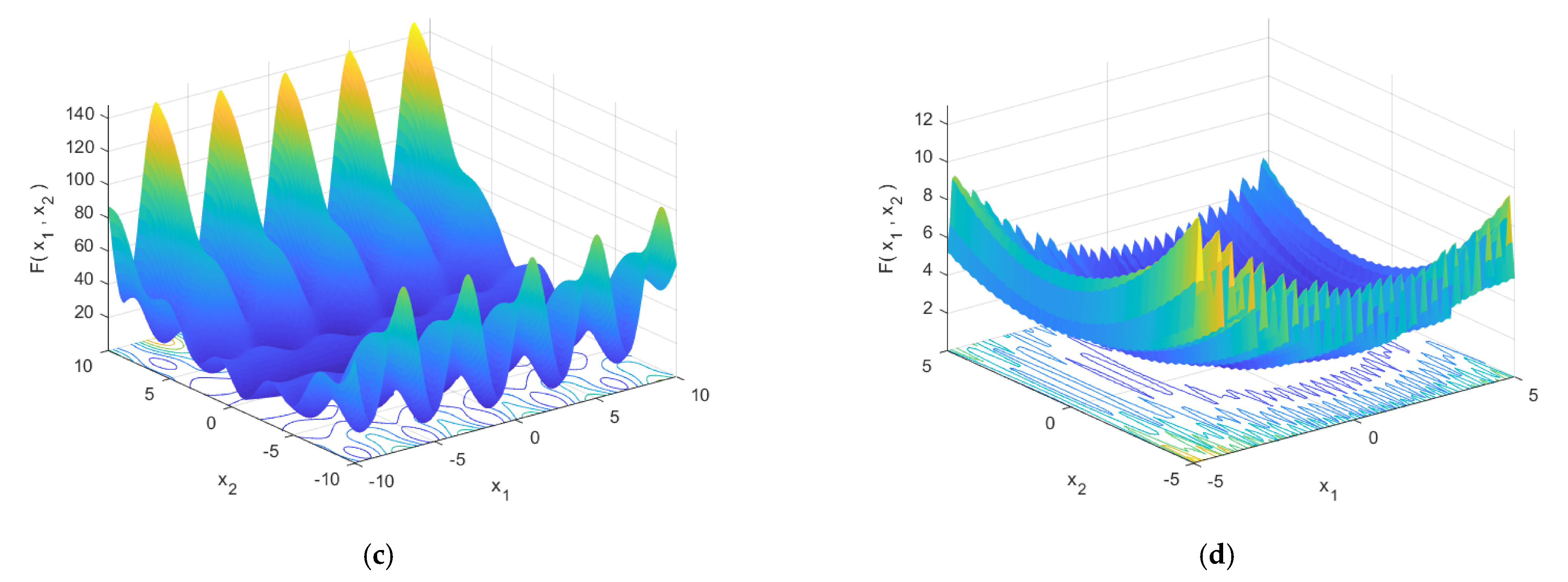
A high-latitude test function is one whose search space dimensionality is relatively high. To demonstrate the optimization-seeking effects of the improved INFO algorithm on high-latitude single-objective test functions, six of the 14 single-objective types were selected for testing. Their convergence curves are shown in Figure 2, and their optimization-seeking space diagrams are shown in Figure 3. INFO1 represents an improved strategy that introduces two-stage backward learning and a greedy mechanism in the original INFO algorithm. INFO2 represents an improved strategy that introduces a differential evolution algorithm and an adaptive t-distribution in the original INFO algorithm. The results for INFO1 and INFO2 are illustrated in Figure 4 and Figure 5, respectively.

To verify the efficacy of IDEINFO, ablation experiments based on INFO1 and INFO2 were conducted for comparison. In this test,INFO1 represents an improved strategy that introduces two-stage backward learning and a greedy mechanism in the original INFO algorithm.INFO2 represents an improved strategy that introduces a differential evolution algorithm and an adaptive t-distribution in the original INFO algorithm.

3.2.2. High-Dimensional Multi-Objective Test Function

To demonstrate the optimization-seeking effects of the improved INFO algorithm on high-latitude multi-objective test functions, four more of the 14 test functions were selected for testing. Their convergence curves are shown in Figure 6, and their optimization-seeking space diagrams are shown in Figure 7. The results for INFO1 and INFO2 are shown in Figure 8 and Figure 9, respectively. As above, in this test, INFO1 represents an improved strategy that introduces two-stage backward learning and a greedy mechanism in the original INFO algorithm, and INFO2 represents an improved strategy that introduces a differential evolution algorithm and an adaptive t-distribution in the original INFO algorithm.

To verify the efficacy of IDEINFO, ablation experiments based on INFO1 and INFO2 were conducted for comparison. INFO1 represents an improved strategy that introduces two-stage backward learning and a greedy mechanism in the original INFO algorithm.INFO2 represents an improved strategy that introduces a differential evolution algorithm and an adaptive t-distribution in the original INFO algorithm.

3.2.3. Low-Dimensional Test Functions

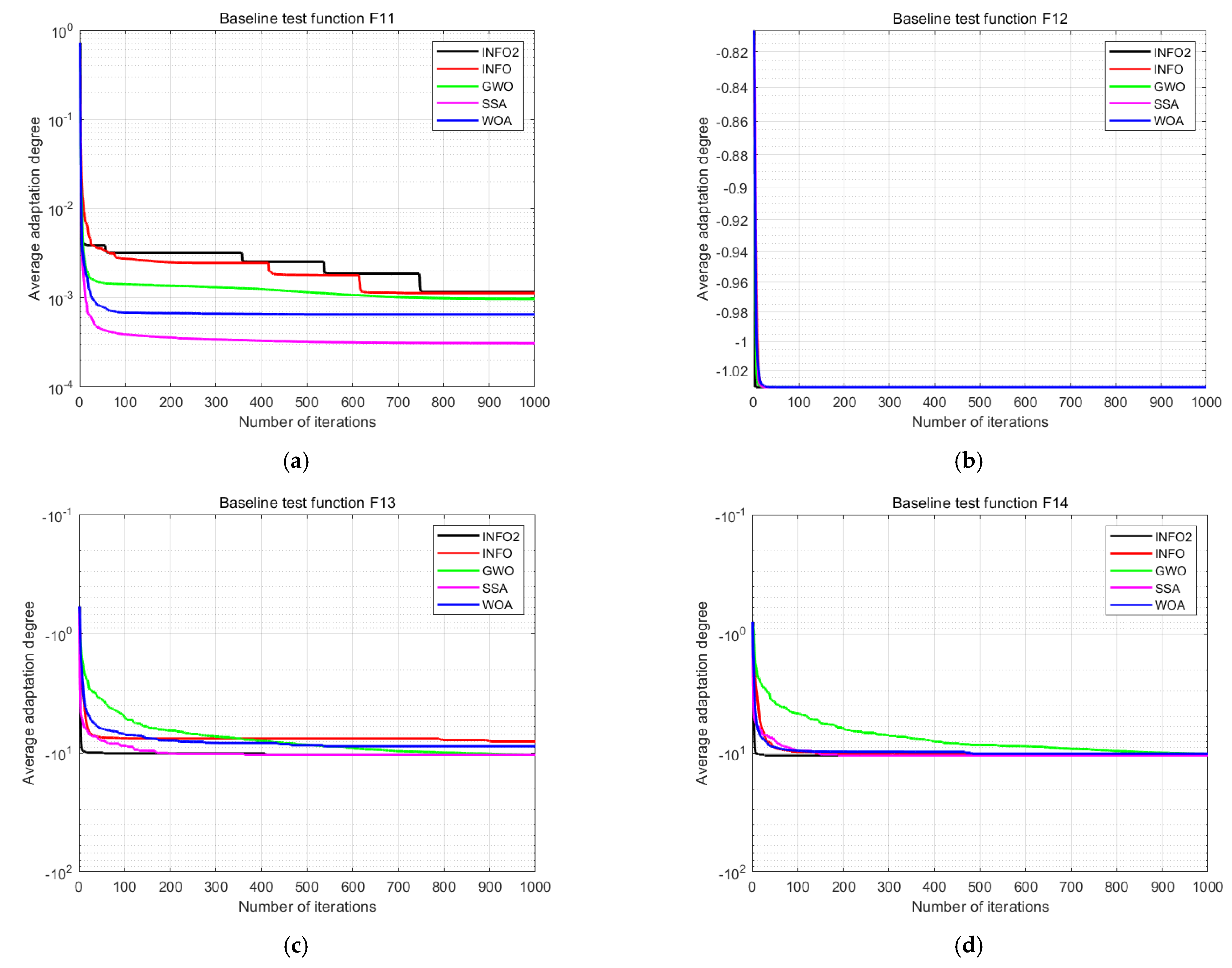
A low-latitude test function is one whose search space dimensionality is relatively low. To demonstrate the optimization-seeking effects of the improved INFO algorithm on low-latitude test functions, the last four of the 14 functions were selected for testing. Their convergence curves are shown in Figure 10, and their optimization-seeking space diagrams are presented in Figure 11. As above, INFO1 represents an improved strategy that introduces two-stage backward learning and a greedy mechanism in the original INFO algorithm, while INFO2 represents an improved strategy that introduces a differential evolution algorithm and an adaptive t-distribution in the original INFO algorithm. The results graphs for INFO1 and INFO2 are illustrated in Figure 12 and Figure 13, respectively.

To verify the efficacy of IDEINFO, ablation experiments based on INFO1 and INFO2 were conducted for comparison. INFO1 represents an improved strategy that introduces two-stage backward learning and a greedy mechanism in the original INFO algorithm.INFO2 represents an improved strategy that introduces a differential evolution algorithm and an adaptive t-distribution in the original INFO algorithm.

4. Discussion

4.1. Comparison of Convergence Results

Table 4. Experimental results for six high-latitude single-target benchmark test functions.

F	Index	IDEINFO	INFO	SSA	GWO	WOA	INFO1	INFO2
F1	Best	0	6.7057 × 10−28	0	2.7058 × 10−36	1.3810 × 10−115	4.2970 × 10−28	0
	Mean	0	2.8115 × 10−27	6.4300 × 10−20	1.0693 × 10−34	2.5704 × 10−102	2.8729 × 10−27	0
	Std	0	6.8192 × 10−28	7.2766 × 10−19	1.0672−34	2.1129 × 10−101	6.3544 × 10−28	0
F2	Best	0	1.2106 × 10−53	0	6.3897 × 10−21	9569.1641	9.2088 × 10−54	0
	Mean	0	7.8038 × 10−52	4.2017 × 10−34	1.4629 × 10−14	20,730.2593	7.6727 × 10−52	0
	Std	0	7.0452 × 10−52	5.9418 × 10−33	5.7738 × 10−14	2569.6795	8.3436 × 10−52	0
F3	Best	0	3.4184 × 10−29	0	2.9501 × 10−16	0.00011002	5.7132 × 10−29	0
	Mean	0	5.7937 × 10−28	1.1195 × 10−20	1.7655 × 10−14	32.8655	5.2304 × 10−28	0
	Std	0	3.4028 × 10−28	1.4256 × 10−19	3.4399 × 10−14	28.2881	2.51 × 10−28	0
F4	Best	4.6904 × 10−15	16.9501	2.2361 × 10−11	25.0954	26.1798	16.5694	3.1549 × 10−14
	Mean	1.5759 × 10−8	19.4498	2.5536 × 10−5	26.7773	27.1942	19.4832	1.5887 × 10−8
	Std	3.6914 × 10−8	0.7041	6.0245 × 10−5	0.7764	0.5283	0.7499	6.1874 × 10−8
F5	Best	1.2326 × 10−32	2.6038 × 10−20	4.009 × 10−11	1.2798 × 10−5	0.0092902	1.1449 × 10−19	1.5407 × 10−32
	Mean	3.2376 × 10−31	2.0788 × 10−13	1.2121 × 10−7	0.6228	0.068798	1.9366 × 10−14	7.0196 × 10−31
	Std	5.1236 × 10−31	1.0668 × 10−12	3.522 × 10−7	0.42264	0.078427	6.2517 × 10−14	1.1262 × 10−30
F6	Best	6.2313 × 10−7	5.1252 × 10−5	1.4029 × 10−0	0.00013678	4.3456 × 10−5	6.7265 × 10−0	7.2831 × 10−6
	Mean	7.2422 × 10−5	0.00077635	0.00077635	0.00075583	0.0015206	0.00084333	6.5934 × 10−5
	Std	5.6658 × 10−5	0.00066449	0.00066449	0.00044961	0.0016606	0.00073516	4.0882 × 10−5

,

Table 5. Experimental results for four high-latitude multi-objective benchmark test functions.

F	Index	IDEINFO	INFO	SSA	GWO	WOA	INFO1	INFO2
F7	Best	−11205.917	−11365.255	−12569.485	−7610.723	−12569.482	−10928.05	−12094.216
	Mean	−10218.713	−8662.457	−9140.772	−5864.470	−11201.082	−9034.592	−10451.007
	Std	592.216	731.942	2642.386	717.885	1541.727	641.344	617.033
F8	Best	4.4409 × 10−16	4.4409 × 10−16	4.4409 × 10−16	1.1102 × 10−14	4.4409 × 10−16	4.4409 × 10−16	4.4409 × 10−16
	Mean	4.4409 × 10−16	4.4409 × 10−16	4.4409 × 10−16	1.5881 × 10−14	3.6948 × 10−15	4.4409 × 10−16	4.4409 × 10−16
	Std	0	0	0	2.8846 × 10−15	2.4875 × 10−15	0	0
F9	Best	1.7077 × 10−32	3.4691 × 10−21	7.7964 × 10−14	0.0062327	0.00062453	4.7647 × 10−21	1.6593 × 10−32
	Mean	1.1726 × 10−30	0.0062119	8.5844 × 10−9	0.037611	0.0074199	0.0031101	1.3445 × 10−31
	Std	2.7026 × 10−30	0.028725	2.0196 × 10−8	0.020538	0.0087554	0.017729	5.8543 × 10−31
F10	Best	0.043939	1.0754 × 10−18	7.0359 × 10−12	4.5913 × 10−5	0.012006	4.5503 × 10−19	0.043939
	Mean	1.2208	0.050698	1.417 × 10−7	0.51788	0.21943	0.057427	1.2345
	Std	1.1314	0.07418	3.8101 × 10−7	0.22404	0.15429	0.06979	1.1609

and

Table 6. Experimental results for four low-latitude benchmark test functions.

F	Index	IDEINFO	INFO	SSA	GWO	WOA	INFO1	INFO2
F11	Best	0.00030749	0.00030749	0.00030749	0.00030749	0.00030752	0.0030749	0.00030749
	Mean	0.0011592	0.00033496	0.00031349	0.0010126	0.00058225	0.0043524	0.0041142
	Std	0.0003646	0.0001566	6.6315 × 10−5	0.0037102	0.00040975	0.0014248	0.00032207
F12	Best	−1.0316	−1.0316	−1.0316	−1.0316	−1.0316	−1.0316	−1.0316
	Mean	−1.0316	−1.0316	−1.0316	−1.0316	−1.0316	−1.0316	−1.0316
	Std	6.7752 × 10−16	6.7752 × 10−16	3.905 × 10−9	4.2802 × 10−9	1.3367 × 10−10	6.7122 × 10−16	6.7122 × 10−16
F13	Best	−10.4029	−10.4029	−10.4029	−10.4029	−10.4027	−10.4029	−10.4029
	Mean	−10.4029	−8.6849	−10.4029	−10.4028	−8.1503	−8.6849	−9.7031
	Std	1.8067 × 10−15	3.1747	1.2781 × 10−5	9.0224 × 10−5	3.1151	3.1747	2.1403
F14	Best	−10.5364	−10.5364	−10.5364	−10.5364	−10.5364	−10.5364	−10.5364
	Mean	−10.5364	−9.8192	−10.5364	−10.5363	−9.4995	−10.0462	−10.313
	Std	1.6493 × 10−15	2.1989	1.8401 × 10−5	8.0884 × 10−5	2.3942	1.8886	1.2234

present the summary analysis of the results of testing high-latitude single-target, high-latitude multi-target, and low-latitude benchmark functions. From these tables, it can be seen that the improved INFO algorithm has the best results, and comparison tests with INFO1 and INFO2 show that the improved method provides superior accuracy and robustness. For the high-dimensional test function, the experimental results in Table 4 show that, in general, the difference between IDEINFO and INFO2 is not significant, but IDEINFO has the highest optimization accuracy among the six compared algorithms, and the solution accuracy and stability of IDEINFO are significantly better than the five comparison algorithms. The experimental results in Table 5 show that IDEINFO has the highest overall. However, among the F9 functions, INFO2 outperforms the other comparative algorithms.

In the low-dimensional test functions, as shown in Table 6, the IDEINFO algorithm proposed in this paper significantly outperforms the other six algorithms, and the optimal solution is found for each of the compared algorithms in the optimization experiment for the F12 function. Therefore, it is verified that the IDEINFO algorithm is highly robust in solving low- and high-dimensional problems, demonstrating that the IDEINFO algorithm has some competitive advantage in solving function optimization problems.

4.2. Wilcoxon Rank Sum Test

In the above simulation experiment, the mean and standard deviation alone cannot fully verify the superiority of the IDEINFO algorithm. To ensure the fairness and validity of the algorithm, it is necessary to conduct a statistical test. In this paper, we use the Wilcoxon rank sum test to verify whether the results of each IDEINFO experiment are statistically significantly different from other algorithms. The rank sum test was performed at the 5% significance level, and at p < 5%, it can be considered as rejecting the H0 hypothesis, indicating that there is a significant difference between the two algorithms; for p > 5%, the H0 hypothesis is accepted, indicating that the two algorithms have the same overall performance.

Table 7. Wilcoxon rank sum test results.

F	Index	INFO	SSA	GWO	WOA	INFO1	INFO2
F1	P	6.3864× 10−5	0.00023125	6.3864× 10−5	6.3864× 10−5	6.3864× 10−5	NaN
	R	+	+	+	+	+	=
F2	P	6.3864× 10−5	0.00075118	6.3864× 10−5	6.3864× 10−5	6.3864× 10−5	NaN
	R	+	+	+	+	+	=
F3	P	6.3864× 10−5	6.3864× 10−5	6.3864× 10−5	6.3864× 10−5	6.3864× 10−5	NaN
	R	+	+	+	+	+	=
F4	P	0.00018267	0.00018267	0.00018267	0.00018267	0.00018267	0.73373
	R	+	+	+	+	+	-
F5	P	0.00018165	0.00018165	0.00018165	0.00018165	0.00018165	1
	R	+	+	+	+	+	-
F6	P	0.00018267	0.001008	0.00018267	0.00018267	0.00018267	0.57075
	R	+	+	+	+	+	-
F7	P	0.00018165	0.14047	0.00018267	0.79134	0.00018165	0.47268
	R	+	-	+	-	+	-
F8	P	0.00018165	NaN	4.0402 × 10−5	0.00018923	0.00018165	NaN
	R	+	=	+	+	+	=
F9	P	0.00018267	0.00018267	0.00018267	0.00018267	0.00018267	0.42736
	R	+	+	+	+	+	-
F10	P	0.00018267	0.021134	0.14047	0.00018267	0.00018267	0.8796
	R	+	+	-	+	+	-
F11	P	0.00017562	0.00017562	0.00017562	0.00017562	0.00017562	0.010336
	R	+	+	+	+	+	+
F12	P	6.3864 × 10−5	6.3864 × 10−5	6.3864 × 10−5	6.3864 × 10−5	6.3864 × 10−5	NaN
	R	+	+	+	+	+	=
F13	P	6.3864 × 10−5	6.3864 × 10−5	6.3864 × 10−5	6.3864 × 10−5	6.3864 × 10−5	NaN
	R	+	+	+	+	+	=
F14	P	0.00010997	0.00010997	0.00010997	0.00010997	0.00010997	0.58278
	R	+	+	+	+	+	-

compares the IDEINFO, INFO1, INFO2,INFO, SSA, WOA, and GWO algorithms for 14 benchmark tests. The Wilcoxon rank sum test on 14 benchmark functions is presented in Table 7. It indicates the comparable performance between the two, where “Na” is “not applicable”; i.e., no significant test can be performed. For the results of the significance tests, “+”, “−”, and “=”, indicate that the performance of IDEINFO is better or worse than that of the compared algorithm.

As shown in Table 7, most of the p-values are less than 5%, and the overall performance of IDEINFO is statistically significantly different from the other six algorithms, thus indicating that IDEINFO has better performance than the other algorithms.

5. Conclusions

This study proposed an improved INFO algorithm that overcomes the shortcomings of the traditional version. The new version initializes candidate solutions using a two-stage backward learning strategy, which improves the uniformity of their distribution and enhances the search capability of the algorithm. The new INFO algorithm is augmented by combining it with a greedy search algorithm, which results in improved individual vectors per iteration and an improved search capacity. During the iterative search process, a DE strategy is applied to perturb the vectors and generate genetically superior candidate solutions. Furthermore, the search range is expanded probabilistically and combined with a t-distribution strategy, which helps avoid local optima traps and improves the global search capability. Using fourteen standard test functions, the improved INFO outperformed the baseline INFO, SSA, GWO, and WOA models. To further verify the efficacy of the improvement points, comparisons were made with INFO1, which performs only two-stage backward learning and a greedy mechanism, and INFO2, which only performs the combined DE and adaptive t-distribution actions. The ablative results show that the proposed improved INFO algorithm has better generality, whereas the others present limitations. In the future, we plan to determine how to balance the time and optimization capabilities of the new algorithm, improve its stability, and find practical applications. The convergence rate of IDEINFO proposed in this paper is very impressive because the position of the vectors always tends to move toward the region where a better solution is available. In addition, the IDEINFO algorithm can solve practically complex and challenging optimization problems with constrained and unknown search domains.

For future research, we suggest the following corrections and considerations. Moreover, we suggest enhancing INFO using different types of local search operators in the original INFO; this may further improve the algorithm’s optimality seeking ability and its capability to address the challenging nature of complex scenarios. The IDEINFO algorithm proposed in this paper can also be enriched in terms of exploratory and exploitative trends. For example, using different concepts, such as chaotic mapping, could enrich the exploratory and exploitative trends of the proposed IDEINFO. The traditional INFO, or its improved variants, can be applied to applications such as parameter tuning in neural network models, effect enhancement of model prediction methods, and deep learning.

References

- Su, Y.; Han, L.; Wang, H.; Wang, J. The workshop scheduling problems based on data mining and particle swarm optimization algorithm in machine learning areas. Enterp. Inf. Syst. 2022, 2, 363–378. [Google Scholar] [CrossRef]
- Mou, J.; Duan, P.; Gao, L.; Liu, X.; Li, J. An effective hybrid collaborative algorithm forenergy-efficient distributed permutation flow-shop inverse scheduling. Future Gener. Comput. Syst. 2022, 128, 521–537. [Google Scholar] [CrossRef]
- Berkan, A.I. A hybrid firefly and particle swarm optimization algorithm for computationally expensive numerical problems. App. Soft Comput. 2018, 66, 232–249. [Google Scholar]
- Zhang, J.; Kewen, X.; Ziping, H.; Shurui, F. Dynamic multi-swarm differential learning quantum bird swarm algorithm and its application in random forest classification model. Comput. Intell. Neurosci. 2020, 2020, 6858541. [Google Scholar] [CrossRef]
- Zhang, M.; Yu, C.; Jingqiang, L. A privacy-preserving optimization of neighborhood-based recommendation for medical-aided diagnosis and treatment. IEEE Internet Things J. 2021, 8, 10830–10842. [Google Scholar] [CrossRef]
- Pallonetto, F.; De Rosa, M.; Finn, D.P. Impact of intelligent control algorithms on demand response flexibility and thermal comfort in a smart grid ready residential building. Smart Energy 2021, 2, 100017. [Google Scholar] [CrossRef]
- Yongbin, Y.; Yang, C.; Deng, Q.; Nyima, T.; Liang, S.; Zhou, C. Memristive network-basedgenetic algorithm and its application to image edge detection. J.Syst. Eng. Electron. 2021, 32, 1062–1070. [Google Scholar] [CrossRef]
- Ai, N.; Bin, W.; Boyu, L.; Zhipeng, Z. 5G heterogeneous network selection and resource allocation optimization based on cuckoo search algorithm. Comput. Comm. 2021, 168, 170–177. [Google Scholar] [CrossRef]
- Passino, K.M. Biomimicry of bacterial foraging for distributed optimization and control. IEEE Control Sys. 2002, 22, 52–67. [Google Scholar]
- Holland John, H. Adaptation in Natural and Artificial Systems:An Introductory Analysis with Applications to Biology, Control, and Artificial Intelligence; The MIT Press: Cambridge, MA, USA, 1992. [Google Scholar]
- Holland, J.H. Genetic algorithms. Sci. Am. 1992, 267, 66–73. [Google Scholar] [CrossRef]
- Knowles, J.; Corne, D. The Pareto archived evolution strategy: A new baseline algorithm for Pareto multiobjective optimization. In Proceedings of the 1999 Congress on Evolutionary Computation-CEC99 (Cat. No. 99TH8406), Washington, DC, USA, 6–9 July 1999. [Google Scholar]
- Kirkpatrick, S.; Gelatt, C.D.; Vecchi, M.P. Optimization by simulated annealing. Science 1983, 220, 671–680. [Google Scholar] [CrossRef]
- Eker, E.; Kayri, M.; Ekinci, S.; Izci, D. A New Fusion of ASO with SA Algorithm and Its Applications to MLP Training and DC Motor Speed Control. Arab. J. Sci. Eng. 2021, 46, 3889–3911. [Google Scholar] [CrossRef]
- Mirjalili, S.; Mirjalili, S.M.; Lewis, A. Grey wolf optimizer. Adv. Eng. Softw. 2014, 69, 46–61. [Google Scholar] [CrossRef]
- Saxena, A.; Kumar, R.; Das, S. β-chaotic map-enabled grey wolf optimizer. Appl. Soft Comput. 2019, 75, 84–105. [Google Scholar] [CrossRef]
- Ahmadianfar, I.; Bozorg-Haddad, O.; Chu, X. Gradient-based optimizer: A new metaheuristic optimization algorithm. Information Sciences 2020, 540, 131–159. [Google Scholar] [CrossRef]
- Li, S.P.; Sun, Y.Z.; Xiaohui, W. Speech Emotion Recognition Using Hybrid GBO Algorithm-based ANFIS Classifier. Indian J. Pharm. Sci. 2019, 81, S52–S53. [Google Scholar]
- Kadkhodazadeh, M.; Farzin, S. A Novel LSSVM Model Integrated with GBO Algorithm to Assessment of Water Quality Parameters. Water Resources Management 2021, 35, 3939–3968. [Google Scholar] [CrossRef]
- Zhangfang, H. Improved particle swarm optimization algorithm for mobile robot path planning. Comput. Appl. Res. 2021, 38, 3089–3092. [Google Scholar]
- Yuxiang, H.; Huanbing, G.; Zijian, W.; Chuansheng, D. Improved Grey Wolf Optimization Algorithm and Application. Sensors 2022, 22. [Google Scholar]
- Khan, M.K.; Zafar, M.H.; Rashid, S.; Mansoor, M.; Moosavi, S.K.R.; Sanfilippo, F. Improved Reptile Search Optimization Algorithm: Application on Regression and Classification Problems. App. Sci. 2023, 13, 945. [Google Scholar] [CrossRef]
- Ayyarao, T.S.; Ramakrishna, N.; Elavarasan, R.M.; Polumahanthi, N.; Rambabu, M.; Saini, G.; Khan, B.; Alatas, B. War Strategy Optimization Algorithm: A New Effective Metaheuristic Algorithm for Global Optimization. IEEE Access 2022, 10, 25073–25105. [Google Scholar] [CrossRef]
- Wolpert, D.H.; Macready, W.G. No free lunch theorems for optimization. IEEE Trans. Evol.Comput. 1997, 1, 67–82. [Google Scholar] [CrossRef]
- Service, T.C. A No Free Lunch theorem for multi-objective optimization. Inf. Process. Lett. 2010, 110, 917–923. [Google Scholar] [CrossRef]
- Iman, A.; Heidari, A.A.; Noshadian, S.; Chen, H.; Gandomi, A.H. INFO: An efficient optimization algorithm based on weighted mean of vectors. Expert Syst. Appl. 2022, 195, 116516. [Google Scholar]
- Akyol, S.; Alatas, B. Plant intelligence based metaheuristic optimization algorithms. Artif. Intell. Rev. 2017, 47, 417–462. [Google Scholar] [CrossRef]
- Dorigo, M.; Maniezzo, V.; Colorni, A. Ant system: Optimization by a colony of cooperating agents. IEEE transactions on systems, man, and cybernetics. Part B Cybern. A Publ. IEEE Syst. Man Cybern. Soc. 1996, 26, 29–41. [Google Scholar] [CrossRef]
- Karaboga, D.; Basturk, B. A powerful and efficient algorithm for numerical function optimization: Artificial bee colony (ABC) algorithm. J. Glob. Optim. 2007, 39, 459–471. [Google Scholar] [CrossRef]
- Heidari, A.A.; Abbaspour, R.A.; Chen, H. Efficient boosted grey wolf optimizers for global search and kernel extreme learning machine training. J. App. Soft Comput. 2019, 81, 105521. [Google Scholar] [CrossRef]
- Yang, Y.; Chen, H.; Heidari, A.A.; Gandomi, A.H. Hunger games search: Visions, conception, implementation, deep analysis, perspectives, and towards performance shifts. Expert Syst. Appl. 2021, 177, 114864. [Google Scholar] [CrossRef]
- Ahmadianfar, I.; Heidari, A.A.; Gandomi, A.H.; Chu, X.; Chen, H. RUN beyond the metaphor: An efficient optimization algorithm based on Runge Kutta method. Expert Syst. Appl. 2021, 181, 115079. [Google Scholar] [CrossRef]
- Li, S.; Chen, H.; Wang, M.; Heidari, A.A.; Mirjalili, S. Slime mould algorithm: A new method for stochastic optimization. Future Gener. Comput. Syst. 2020, 111, 300–323. [Google Scholar] [CrossRef]
- Mirjalili, S.; Lewis, A. The Whale Optimization Algorithm. Adv. Eng. Softw. 2016, 95, 51–67. [Google Scholar] [CrossRef]
- Bonyadi, M.R.; Michalewicz, Z. Particle Swarm Optimization for Single Objective Continuous Space Problems: A Review. Evol. Comput. 2017, 25, 1–54. [Google Scholar] [CrossRef] [PubMed]
- Jwad, K.I.; Yuegang, T.; Layth, Q. Integration of DE Algorithm with PDC-APF for Enhancement of Contour Path Planning of a Universal Robot. App. Sci. 2021, 11, 6532. [Google Scholar]
- Ghiasi, M.; Niknam, T.; Dehghani, M.; Siano, P.; Haes, A.H.; AlHinai, A. Optimal Multi-Operation Energy Management in Smart Microgrids in the Presence of RESs Based on Multi-Objective Improved DE Algorithm: Cost-Emission Based Optimization. Appl. Sci. 2021, 11, 3661. [Google Scholar] [CrossRef]
- Shihong, Y.; Qifang, L.; Yanlian, D.; Yongquan, Z. DTSMA: Dominant Swarm with Adaptive T-distribution Mutation-based Slime Mould Algorithm. Math. Biosci. Eng. 2022, 19, 2240–2285. [Google Scholar]
- Coufal, P.; Hubálovský, Š.; Hubálovská, M.; Balogh, Z. Snow Leopard Optimization Algorithm: A New Nature-Based Optimization Algorithm for Solving Optimization Problems. Mathematics 2021, 9, 2832. [Google Scholar] [CrossRef]
Figure 1.
Steps of improving the INFO algorithm based on two-stage backward learning DE and t-distribution strategies.
Figure 2.
Convergence curves of six selected high-dimensional single-objective test functions: (a) F1, (b) F2, (c) F3, (d) F4, (e) F5, and (f) F6.
Figure 3.
Optimization-seeking space diagrams for six selected high-dimensional single-objective test functions: (a) F1, (b) F2, (c) F3, (d) F4, (e) F5, and (f) F6.
Figure 4.
Results for six selected high-dimensional single-objective test functions: (a) F1, (b) F2, (c) F3, (d) F4, (e) F5, and (f) F6.
Figure 5.
Figure 6.
Convergence curves of four selected high-dimensional multi-objective test functions: (a) F7, (b) F8, (c) F9, and (d) F10.
Figure 7.
Optimization-seeking space diagrams for four selected high-dimensional multi-objective test functions: (a) F7, (b) F8, (c) F9, and (d) F10.
Figure 8.
Results for four selected high-dimensional multi-objective test functions (a) F7, (b) F8, (c) F9, and (d) F10.
Figure 9.
Figure 10.
Convergence curves of four selected low-dimensional test functions: (a) F11, (b) F12, (c) F13, and (d) F14.
Figure 11.
Optimization-seeking space diagrams for four selected low-dimensional test functions: (a) F11, (b) F12, (c) F13, and (d) F14.
Figure 12.
Results for four selected low-dimensional test functions (a) F11, (b) F12, (c) F13, and (d) F14.
Figure 13.