Dynamics of a 3-UPS-UPU-S Parallel Mechanism

Abstract

In this paper, a parallel mechanism with two rotational degrees of freedom is proposed. It could rotate freely and continuously around the two coordinate axes at the fixed origin of the coordinate frame. The structure of the mechanism is a second-order over constraint parallel structure and the moving platform and base platform are connected by five kinematic chains. The motion characteristics of this structure are analyzed by reciprocal screw equation. Then, the kinematics and dynamics modelling are carried out systematically in a unified way. The kinematics of the mechanism is established by means of screws, the displacements and accelerations of each joint and any point on a link could be calculated by the kinematic screw equation directly. The analysis of acceleration and its mathematical expression in screw form are given, and the acceleration matrix could be applied into the dynamic analysis based on the Newton–Euler equation. All the constraint forces and torques could be obtained by a single set of Newton–Euler equations.

1. Introduction

Compared with its serial counterparts, a parallel mechanism provides higher load-bearing capability and can be precisely controlled with a quick response and adjustment [1]. Hence, parallel mechanisms have been commonly applied in equipment and mechanisms with large scalar and mission requirements to be heavy duty, which requires higher dynamic performance, higher structural stability and robustness and also accurate positioning and lower complexity in control.

For parallel mechanisms with serial kinematic subchains, the motion characteristics, such as degrees of freedom, workspace and singularities, are fundamental to the design of the kinematic subchains [2,3,4]. These motion parameters can be suggested for the optimization of the design and dynamic properties of the parallel mechanisms [5]. Some researchers have disclosed the influence of the arrangement of the joints. Especially for the universal joints, the motion of the moving platform of the parallel mechanism is relevant to the layout of the joints and the direction of the rotary axes [6]. Then, the kinematic analysis is the basis for gaining the kinematic information of the structure and its controlling and correcting posture [7]. Many researchers have proposed various methods for analyzing the kinematics of parallel mechanisms [8,9,10,11]. As one of those common methods, kinematics and as well as dynamics of mechanism can be studied systematically through the theory of screw. Screw theory is known as a computational, supremely efficient approach to analyze the kinematics, statics and dynamics of mechanisms [12]. The velocities, accelerations of each movable joints on sub chains and any point on moving platform can be obtained, which form the groundwork for further dynamic modelling [13].

Dynamic analysis is one of the kernels of mechanism control [14]. Methods of dynamic modelling have been widely studied, in that it is necessary for determining the forces and moment of joints and actuators. Traditionally, the dynamic analysis is carried out via two kinds of methods: methods based on vectors, such as the Newton–Euler method [15] and on energy, such as methods using Lagrangian equations [16,17,18,19]. The dynamic modelling of parallel mechanisms is often complex and difficult, because it is based on the kinematic information of the mechanisms and dynamic parameters [20]. Conventional dynamics analysis through the Newton–Euler method relies on motion equations of each part of the mechanism. Describing the dynamics with Lagrangian equations is practical in solving the inverse dynamics, but it also requires as much large computation time as the Newton–Euler method does. Ren and Cao obtained the position information of a $3-\mathrm{PSS}$ parallel mechanism through a Jacobian matrix and established the dynamic model using Lagrangian equations [21]. Through the principle of virtual work, the dynamics is expressed by building the energy equations in a generalized coordinate framework and the complexity of analyzing the inverse dynamics can be reduced [22,23,24,25]. Some other methods have also been explored and applied in dynamic analysis such as the recursive matrix method [26], the influence coefficient method, which is separate to the velocity and acceleration variables [27] and the Kane equation [28,29,30]. Jiao et al. established a dynamic model of the Stewart platform through a combination of Kane equation and the principle of virtual works [31]. Considering that screw theory has already been extensively used in dynamic analysis, based on the kinematic formulations through screw theory, dynamics modelling of mechanisms can be established more efficiently [32,33,34]. Garcia-Murillo solved the inverse dynamics of a translational parallel mechanism via screw theory and the virtual work principle [35].

The existing methods of kinematic analysis often start from displacement and the second order numerical differential interpolation is required to calculate the acceleration. Compared with existing methods, the main contributions of this paper are that a novel $3\mathrm{U}\underset{\_}{\mathrm{P}}\mathrm{S-U}\underset{\_}{\mathrm{P}}\mathrm{U-S}$ over a constraint parallel mechanism is proposed to satisfy the motion demands of two rotational degrees of freedom and the displacements, velocities and accelerations are calculated by the velocity screw equation directly. This mathematical expression could simplify the calculation and analysis of dynamics.

2. A Novel 2-Rotational-DoF Parallel Mechanism ($3\mathbf{U}\underset{\_}{\mathbf{P}}\mathbf{S-U}\underset{\_}{\mathbf{P}}\mathbf{U-S}$) and Its DoF

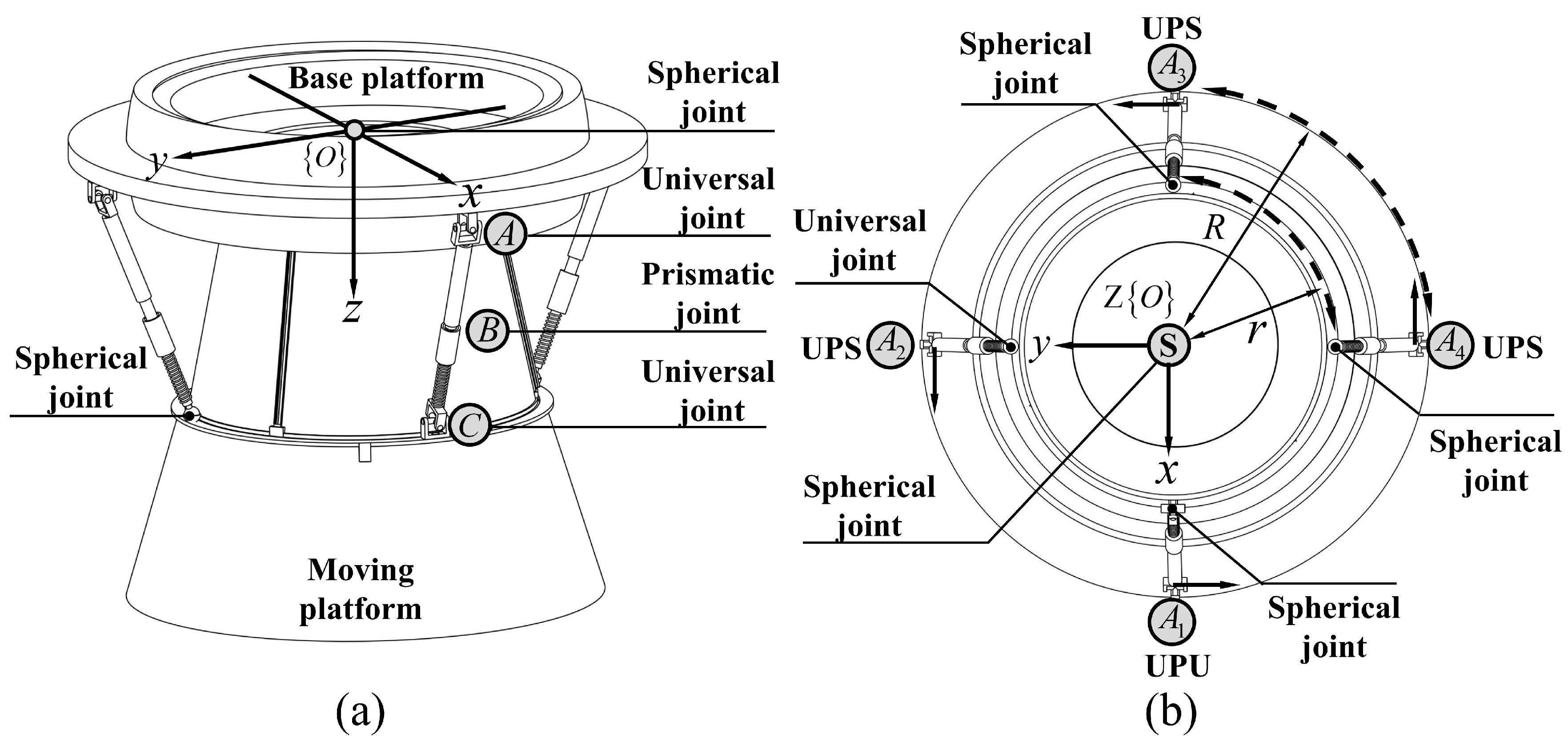
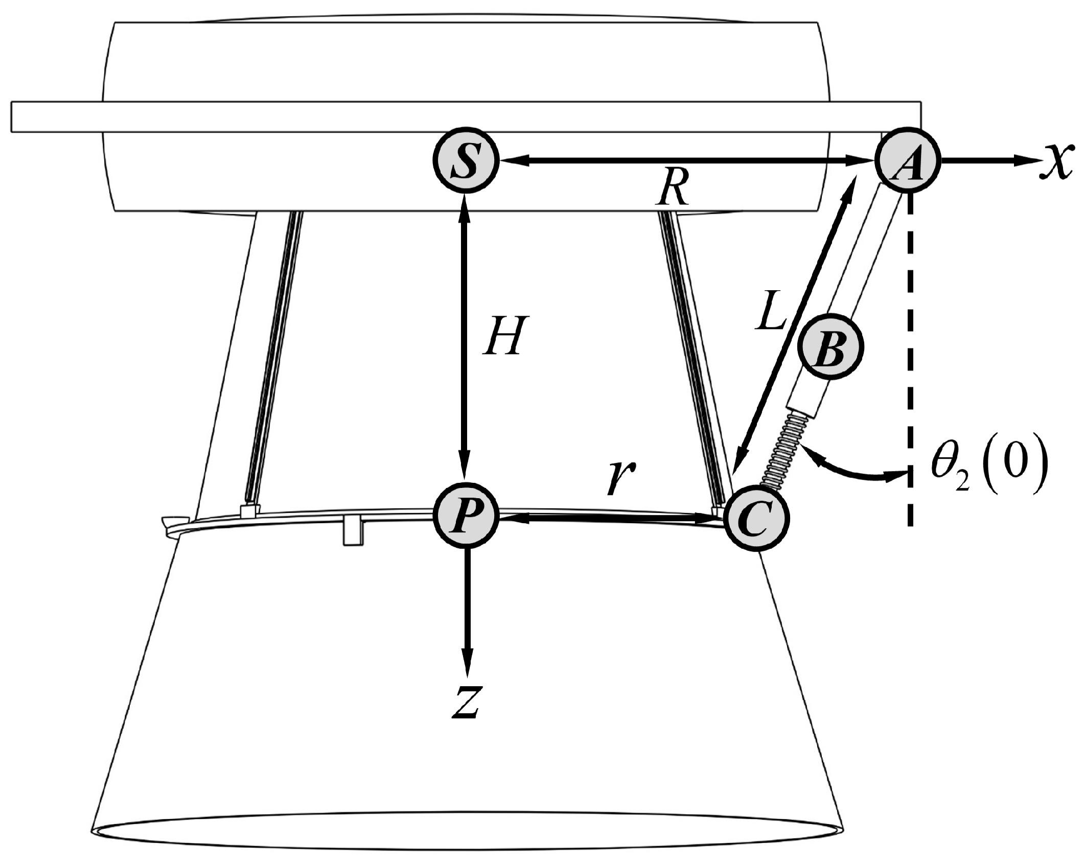
As is shown in Figure 1, a novel 2-rotational-DoF parallel mechanism as a simulator is proposed. This mechanism includes one moving platform, one base platform, and five kinematic chains. Three $\mathrm{U}\underset{\_}{\mathrm{P}}\mathrm{S}$ kinematic chains consist of one universal joint, $\mathrm{U}$, one intermediate prismatic joint, $\underset{\_}{\mathrm{P}}$, as the actuator, and one spherical joint, $\mathrm{S}$. The fourth $\mathrm{U}\underset{\_}{\mathrm{P}}\mathrm{U}$ kinematic chain consists of two universal joints, $\mathrm{U}$, which are connected by one prismatic joint, $\underset{\_}{\mathrm{P}}$. The fifth $\mathrm{S}$ kinematic chain includes only one spherical joint, $\mathrm{S}$, and the revolute center of spherical joint, $\mathrm{S}$, and the geometrical center of the base coincide. The moving platform is directly built into the one with the $\mathrm{S}$ chain. Four kinematic subchains of $3\mathrm{U}\underset{\_}{\mathrm{P}}\mathrm{S-U}\underset{\_}{\mathrm{P}}\mathrm{U}$ are distributed around the spherical joint uniformly. Their primary universal joints are installed along the edge of the base, and the last four joints (universal joint or spherical joints) are assembled on the middle ring of the moving platform. The radii of the circumcircle of $A_1{A}_2{A}_3{A}_4$ and $C_1{C}_2{C}_3{C}_4$ are $R$ and $r$, respectively.

For further analysis, the absolute coordinate $O-xyz$ is set as shown in Figure 1. The origin $O$ is chosen at the center of the base, and the $z$-axis is perpendicular to the base and points to the moving platform; the $x$-axis is along $S{A}_1$ and then through the right-hand rule, the $y$-axis can be settled.

2.1. Fundamentals of Screw Theory

In the following, ${}_{N-1}{}^N\mathit{V}$ is defined to denote the relative velocity screw of joint $J_N$ in the screw coordinate. It consists of the dual 3-dimensional vectors ${}_{N-1}{}^N\mathsf{\omega }$ and ${}_{N-1}{}^N\mathit{v}$, which represent the relative angular velocity and linear velocity, respectively. The velocity screw of joint $J_N$ can be written as

$${}_{N-1}{}^N\mathit{V}=\left[\begin{array}{c}{}_{N-1}{}^N\mathsf{\omega }\\ {}_0{}^N\mathit{r}\times {}_{N-1}{}^N\mathsf{\omega }\end{array}\right]$$

(1)

Equation (1) can also be expressed through the unit vector as

$${}_{N-1}{}^N\mathit{V}={}_{N-1}{}^N\mathsf{\omega }\left[\begin{array}{c}{\mathit{e}}_N\\ {\mathit{r}}_N\times {\mathit{e}}_N\end{array}\right]={}_{N-1}{}^N\mathsf{\omega }{\mathsf{\$}}_N$$

(2)

where ${}_{N-1}{}^N\mathsf{\omega }$ presents the magnitude of the relative angular velocity of the joint $J_N$ with respect to the joint $J_{N-1}$, and ${\mathsf{\$}}_N=\left[\begin{array}{c}{\mathit{e}}_N\\ {\mathit{r}}_N\times {\mathit{e}}_N\end{array}\right]$ is defined as the unit velocity screw and expressed by the unit vector along the joint axis ${\mathit{e}}_N$, whose norm is $\Vert {\mathit{e}}_N\Vert =1$.

The kinematics of a joint in a serial kinematic chain is relative to the kinematics of the fore joints, and the kinematics information of the $N$th joint $J_N$ can be obtained through the linear combination:

$$\{\begin{array}{l}{}_0{}^N\mathsf{\omega }={}_0{}^1\mathsf{\omega }+{}_1{}^2\mathsf{\omega }+{}_2{}^3\mathsf{\omega }+\cdots +{}_{N-2}{}^{N-1}\mathsf{\omega }+{}_{N-1}{}^N\mathsf{\omega }\\ {}_0{}^N\mathit{v}={}_0{}^1\mathit{v}+{}_1{}^2\mathit{v}+{}_2{}^3\mathit{v}+\cdots +{}_{N-2}{}^{N-1}\mathit{v}+{}_{N-1}{}^N\mathit{v}\end{array}$$

(3)

Therefore, based on the kinematic expressions of every joint in a single serial chain through Equation (3), the forward kinematics of the chain can be gained through

$${}_0{}^N\mathit{V}_N={\displaystyle \sum _{i=0}^N{}_i\mathit{V}_{i+1}}=\mathit{S}\mathsf{\omega }$$

(4)

where $\mathit{S}$ represents the unit velocity screw matrix of a series linkage with $N$ joints and is formed by uniting the unit velocity screws of each joint in turns,

$$\mathit{S}=\left[\begin{array}{cccc}{\mathsf{\$}}_1& {\mathsf{\$}}_2& \cdots & {\mathsf{\$}}_N\end{array}\right]$$

(5)

and $\mathsf{\omega }={\left[\begin{array}{cccc}{}_0{}^1\omega & {}_1{}^2\omega & \cdots & {}_{N-1}{}^N\omega \end{array}\right]}^T$ is an angular velocity vector consisting of all relative angular velocities of each joint relative to its previous link in the linkage.

2.2. Reciprocal Screws of Moving Platform and Its DOF

To analyze the DoFs of a parallel mechanism with various kinematic chains, firstly, the mechanism should be divided into chains, and then the constraints of each chain acting on the moving platform should be explained [30,31]. Foremost, the Plücker coordinates of each joint of each chain are carried out based on the absolute coordinate frame as shown in Figure 1a. Therefore, the Plücker coordinates of joints in the $\mathrm{U}\underset{\_}{\mathrm{P}}\mathrm{U}$chain can be written as follows:

$$\begin{array}{l}{\mathsf{\$}}_{UPU}^1={\left[\begin{array}{cccccc}1& 0& 0& 0& 0& 0\end{array}\right]}^T\\ {\mathsf{\$}}_{UPU}^2={\left[\begin{array}{cccccc}0& 1& 0& 0& 0& R\end{array}\right]}^T\\ {\mathsf{\$}}_{UPU}^3={\left[\begin{array}{cccccc}0& 0& 0& -\sin \theta & 0& \cos \theta \end{array}\right]}^T\\ {\mathsf{\$}}_{UPU}^4={\left[\begin{array}{cccccc}\cos \theta & 0& \sin \theta & 0& -R\sin \theta +L& 0\end{array}\right]}^T\\ {\mathsf{\$}}_{UPU}^5={\left[\begin{array}{cccccc}0& 1& 0& -L\cos \theta & 0& R-L\sin \theta \end{array}\right]}^T\end{array}$$

(6)

where $L$ is the length of the kinematic chain, and $\theta$ is angle between the $\mathrm{U}\underset{\_}{\mathrm{P}}\mathrm{U}$ chain and the $z$-axis. Therefore, the screws of the chain are now expressed by

$$\mathrm{S}=\left[\begin{array}{ccccc}{\$}_{UPU}^1& {\$}_{UPU}^2& {\$}_{UPU}^3& {\$}_{UPU}^4& {\$}_{UPU}^5\end{array}\right]$$

(7)

According to the reciprocal screw theory, the inverse screw ${\mathsf{\$}}^r$ can be obtained through

$${\mathit{S}}^T\mathbf{\aleph }{\mathsf{\$}}^r=0$$

(8)

where $\mathbf{\aleph }=\left[\begin{array}{cc}0& {\mathit{I}}_{3\times 3}\\ {\mathit{I}}_{3\times 3}& 0\end{array}\right]$ and ${\mathit{I}}_{3\times 3}=\left[\begin{array}{ccc}1& 0& 0\\ 0& 1& 0\\ 0& 0& 1\end{array}\right]$.

Therefore, the inverse screw of the $\mathrm{U}\underset{\_}{\mathrm{P}}\mathrm{U}$ chain is

$${\mathsf{\$}}_{UPU}^r={\left[\begin{array}{cccccc}0& 1& 0& 0& 0& R-\frac{L}{\sin \theta }\end{array}\right]}^T$$

(9)

Based on screw theory, ${\mathsf{\$}}_{UPU}^r$ can be expressed in a wrench form as ${\mathsf{\$}}_{UPU}^r=\left[\begin{array}{c}\mathit{F}\\ \mathit{r}\times \mathit{F}\end{array}\right]$, and as shown in Equation (9), ${\mathsf{\$}}_{UPU}^r$ is expressed as a force vector parallel to the $y$-axis passing through point $(\begin{array}{ccc}R-\frac{L}{\sin \theta }& b& 0\end{array})$, where $b$ can be any value.

Using the same procedure, the inverse screws of the $\mathrm{U}\underset{\_}{\mathrm{P}}\mathrm{S}$ and $\mathrm{S}$ chains can be obtained

$${\mathsf{\$}}_{UPS}^r={\left[\begin{array}{cccccc}0& 0& 0& 0& 0& 0\end{array}\right]}^T$$

(10)

$${\mathsf{\$}}_S^r={\left[\begin{array}{cccccc}1& 0& 0& 0& 0& 0\\ 0& 1& 0& 0& 0& 0\\ 0& 0& 1& 0& 0& 0\end{array}\right]}^T$$

(11)

Therefore, all the inverse screws provide the terminal constraints to the moving platform:

$${\mathit{S}}_P^C=\left[\begin{array}{cccc}0& 1& 0& 0\\ 1& 0& 1& 0\\ 0& 0& 0& 1\\ 0& 0& 0& 0\\ 0& 0& 0& 0\\ R-\frac{L}{\sin \theta }& 0& 0& 0\end{array}\right]$$

(12)

According to the reciprocal screw Equation (8), the free velocity screws of the moving platform ${\mathsf{\$}}_P$ demonstrate that

$${\left({\mathit{S}}_P^C\right)}^{\mathrm{T}}\aleph {\mathsf{\$}}_P=0$$

(13)

Therefore,

$${\mathsf{\$}}_P={\left[\begin{array}{cccccc}1& 0& 0& 0& 0& 0\\ 0& 1& 0& 0& 0& 0\end{array}\right]}^T$$

(14)

3. The Velocity and Displacement Analysis of the $\mathbf{3}\mathbf{U}\underset{\_}{\mathbf{P}}\mathbf{S-U}\underset{\_}{\mathbf{P}}\mathbf{U-S}$ Parallel Mechanism

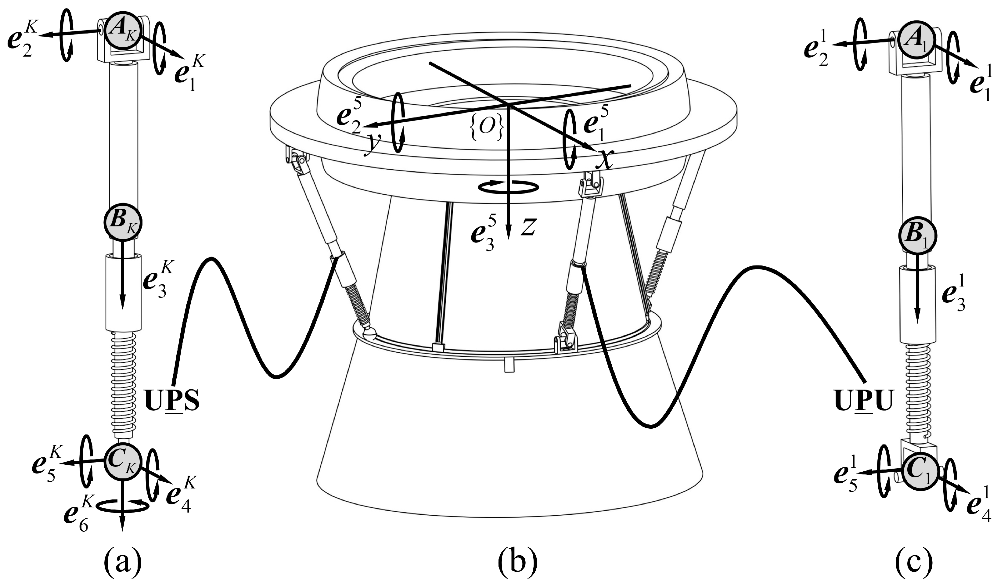
This section gives the kinematic analysis of the $3\mathrm{U}\underset{\_}{\mathrm{P}}\mathrm{S-U}\underset{\_}{\mathrm{P}}\mathrm{U-S}$. As shown in Figure 2b, with the definition of the twist matrix, the kinematic screw equation of a multi-rigid-body system can be obtained through

$$\mathit{S}\mathsf{\omega }=\mathit{V}$$

(15)

with

$$\mathit{S}=\mathrm{diag}{\left[\begin{array}{cccc}{\left[{\mathit{S}}^1\right]}_{6\times 5}& {\left[{\mathit{S}}^2\right]}_{6\times 6}& \cdots & {\left[{\mathit{S}}^5\right]}_{6\times 3}\end{array}\right]}_{30\times 26}$$

(16)

and

$$\mathsf{\omega }={\left[\begin{array}{cccc}{\left[{\mathsf{\omega }}^1\right]}_{5\times 1}^T& {\left[{\mathsf{\omega }}^2\right]}_{6\times 1}^T& \cdots & {\left[{\mathsf{\omega }}^5\right]}_{3\times 1}^T\end{array}\right]}_{26\times 1}^T$$

(17)

where ${\mathsf{\omega }}^N$ is the relative angular velocity vector of each joint of each kinematic chain $looP\left(N\right)$.

${\mathit{S}}^N$ in Equation (16) is the unit screw matrix of the single kinematic chain $looP\left(N\right)$, and $\mathrm{diag}\left[\right]$ means a diagonal matrix with ${\mathit{S}}^1,{\mathit{S}}^2,\cdots ,{\mathit{S}}^5$. As shown in Figure 2a, according to Equation (5), the kinematic unit screw matrix ${\mathrm{S}}^1$ of the $\mathrm{U}\underset{\_}{\mathrm{P}}\mathrm{U}$ chain can be expressed as

$${\mathit{S}}^1=\left[\begin{array}{ccccc}\begin{array}{c}{\mathit{e}}_1^1\\ {\mathit{r}}_A^1\times {\mathit{e}}_1^1\end{array}& \begin{array}{c}{\mathit{e}}_2^1\\ {\mathit{r}}_A^1\times {\mathit{e}}_2^1\end{array}& \begin{array}{c}\mathbf{0}\\ {\mathit{e}}_3^1\end{array}& \begin{array}{c}{\mathit{e}}_4^1\\ {\mathit{r}}_C^1\times {\mathit{e}}_4^1\end{array}& \begin{array}{c}{\mathit{e}}_5^1\\ {\mathit{r}}_C^1\times {\mathit{e}}_5^1\end{array}\end{array}\right]$$

(18)

where $\left[\begin{array}{c}\mathbf{0}\\ {\mathit{e}}_3^1\end{array}\right]$ gives the unit velocity screw of a prismatic joint.

In a similar way, as shown in Figure 2c, the kinematic screw matrix ${\mathit{S}}^K$ of the $K$th $\mathrm{U}\underset{\_}{\mathrm{P}}\mathrm{S}$ chain is

$${\mathit{S}}^K=\left[\begin{array}{cccccc}{\mathit{e}}_1^K& {\mathit{e}}_2^K& \mathbf{0}& {\mathit{e}}_4^K& {\mathit{e}}_5^K& {\mathit{e}}_6^K\\ {\mathit{r}}_A^K\times {\mathit{e}}_1^K& {\mathit{r}}_A^K\times {\mathit{e}}_2^K& {\mathit{e}}_3^K& {\mathit{r}}_C^K\times {\mathit{e}}_4^K& {\mathit{r}}_C^K\times {\mathit{e}}_5^K& {\mathit{r}}_C^K\times {\mathit{e}}_6^K\end{array}\right],\left(K=2,3,4\right)$$

(19)

$${\mathit{S}}^5=\left[\begin{array}{ccc}{\mathit{e}}_1^5& {\mathit{e}}_2^5& {\mathit{e}}_3^5\\ {\mathit{r}}_O^5\times {\mathit{e}}_1^5& {\mathit{r}}_O^5\times {\mathit{e}}_2^5& {\mathit{r}}_O^5\times {\mathit{e}}_3^5\end{array}\right]$$

(20)

The velocity matrix in Equation (15) can be expressed as

$$\mathit{V}={\left[\begin{array}{cccc}{\left[{}_0{}^C\mathit{V}^1\right]}_{6\times 1}^T& {\left[{}_0{}^C\mathit{V}^2\right]}_{6\times 1}^T& \cdots & {\left[{}_0{}^C\mathit{V}^5\right]}_{6\times 1}^T\end{array}\right]}_{30\times 1}^T$$

(21)

where ${}_0{}^C\mathit{V}^K$ contains all the absolute velocity screw of the joints in $K$th kinematic chain.

In addition, the absolute velocity in Equation (19) can be calculated through

$${}_0{}^C\mathit{V}^K={}_0{}^P\mathit{V}-{}_C{}^P\mathit{V}^K$$

(22)

where ${}_0{}^P\mathit{V}$ is the velocity screw of the mass center, $P$, on moving platform which is given in solving the inverse kinematics, and ${}_C{}^P\mathit{V}^K$ is the relative velocity screw of joint $P$ in regard to joint $C$, which can be gained through

$${}_C{}^P\mathit{V}^K=\left[\begin{array}{c}\mathbf{0}\\ {}_0{}^C\mathsf{\omega }^K\times {\mathit{r}}_P^K\end{array}\right]$$

(23)

where ${}_0{}^C\mathsf{\omega }^K$ is the output absolute angular velocity of the $K$th kinematic chain connected with the moving part, while ${\mathit{r}}_P^K$ presents the absolute position of point $P$ in the absolute coordinate frame.

To obtain the required unit screws in Equation (18), the rotation matrix is applied to calculate the unit joint axis, ${\mathit{e}}_n^K$, and the absolute position vector, ${\mathit{r}}_n^K$, of each joint in the absolute coordinate frame:

$$\{\begin{array}{l}{\mathit{e}}_N^K={\mathit{R}}_Z^K\left({\displaystyle \prod _{n=2}{\mathit{R}}_N^K}\right){\mathit{e}}_N^K\left(0\right)\\ {\mathit{r}}_N^K={\mathit{R}}_Z^K\left({}_0\mathit{r}_A^K\left(0\right)+{\mathit{R}}_2^K{\mathit{R}}_3^K{\mathit{R}}_5^K{\mathit{r}}_{AC}^K\right)\end{array},\{\begin{array}{c}\left(N=1,2,\cdots ,4\right)\\ \left(K=1,2,\cdots ,6\right)\end{array}$$

(24)

where ${\mathit{R}}_Z^K$ is the rotation matrix around the $z$-axis, which can be expressed as: ${\mathit{R}}_Z^k=R_Z\left(\left(p-1\right){90}^{\circ }\right)$. ${\mathit{R}}_N^K$ presents the rotation matrix from link $L_N$ to link $L_{N-1}$. When it rotates around x axis, then ${\mathit{R}}_N^K=R_x\left({}_{N-1}\theta _N^K\right)$, and when it rotates around the y axis, ${\mathit{R}}_N^K=R_y\left({}_{N-1}\theta _N^K\right)$, and when it rotates around z axis, ${\mathit{R}}_N^K=R_z\left({}_{N-1}\theta _N^K\right)$.

From Equation (15), if the kinematics of the terminal link $J_N$ is given, the inverse kinematics of the multi-rigid-body system can be derived as

$${\mathit{S}}^T\mathit{S}\mathsf{\omega }={\mathit{S}}^T\mathit{V}$$

(25)

As $\left|{\mathit{S}}^T\mathit{S}\right|=0$, the multi-rigid-body system is either redundantly actuated or in singularity configuration. In another configurations, multiplying both sides of Equation (23) by ${\left[{\mathit{S}}^T\mathit{S}\right]}^{-1}$ yields

$$\mathsf{\omega }={\left[{\mathit{S}}^T\mathit{S}\right]}^{-1}{\mathit{S}}^T\mathit{V}$$

(26)

where ${\left[{\mathit{S}}^T\mathit{S}\right]}^{-1}{\mathit{S}}^T$ is called the pseudo inverse of the screw matrix, $\mathit{S}$. Equation (24) is used to solve the inverse velocity of the linkage.

Obviously, the position $\mathit{r}$ and posture $\mathit{e}$ of each joint are the functions of the angles $\theta$. With the initial assembly conditions, represented through $\mathsf{\theta }\left(0\right)$, the solution of $\mathsf{\omega }\left(1\right)$ can be derived through Equation (24) by substituting $\mathsf{\theta }\left(0\right)$ into the unit screw matrix, $\mathrm{S}$. Then, through an iterative approach, the successive parameters of $\mathit{S}\left(n\right)$ can be obtained by updating the data in Equation (24),

$$\mathsf{\theta }\left(n+1\right)=\mathsf{\theta }\left(n\right)+\Delta t\mathsf{\omega }\left(n\right)$$

(27)

where $\theta \left(n\right)={\left[\begin{array}{ccccc}{}_0{}^1\theta \left(n\right)& {}_1{}^2\theta \left(n\right)& \cdots & {}_{N-2}{}^{N-1}\theta \left(n\right)& {}_{N-1}{}^N\theta \left(n\right)\end{array}\right]}^T$ consists of the angular displacements of all joints, and ${}_{N-1}{}^N\theta$ is the relative angular displacement of joint $J_N$ with respect to joint $J_{N-1}$. $n=1,2,\cdots$ indicates the times of iteration.

4. The Analysis of Acceleration and Its Mathematical Expression

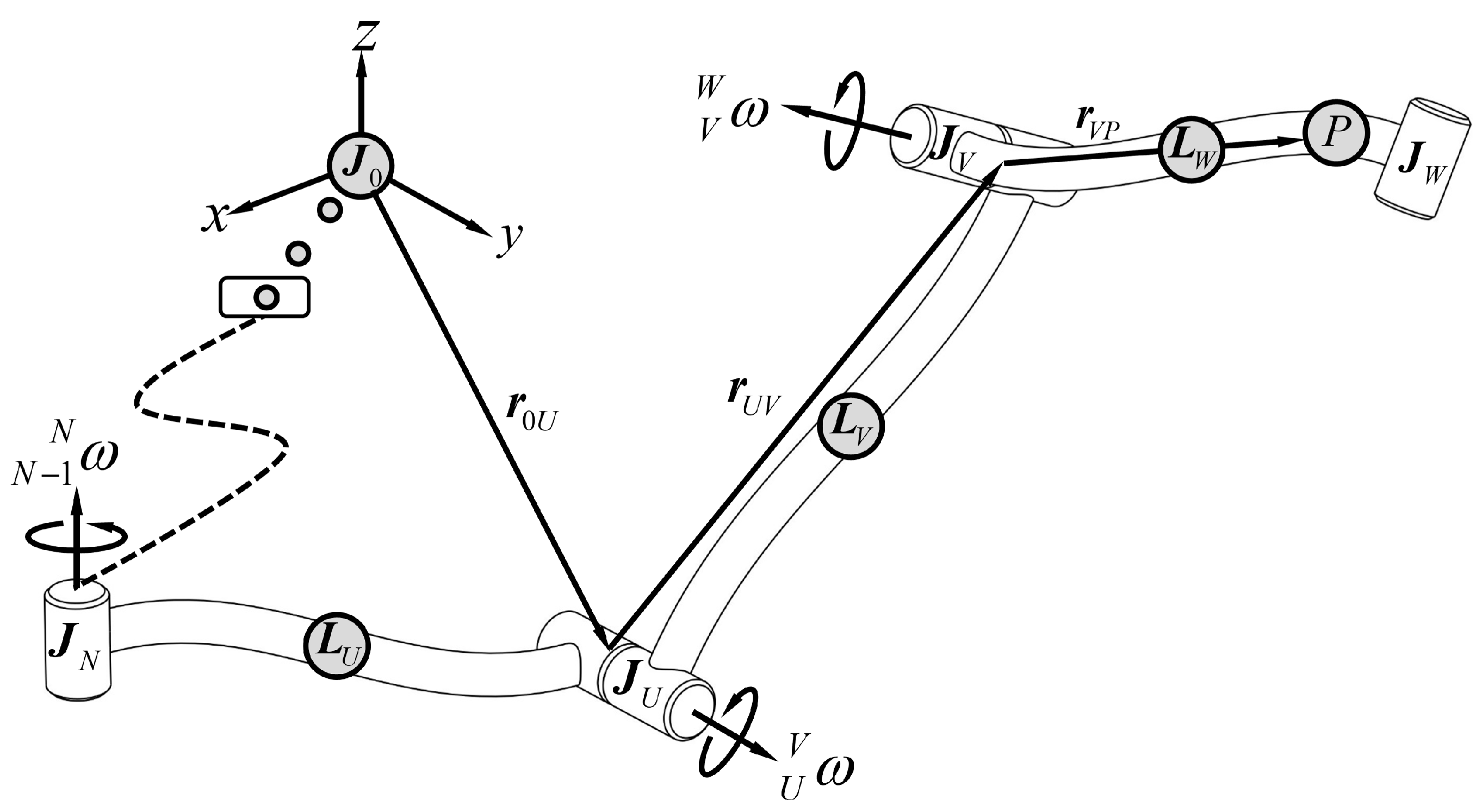
In this section, the analysis of acceleration and its mathematical expression is given. As depicted in Figure 3, suppose that $U$, $V$ and $W$ are three rigid bodies in a serial kinematic chain connected by a number of joints successively, and there is an arbitrary point, $P$, attached to the link $L_W$. Therefore, the velocities of $P$ attached to these two frames observed from frame $U$ are

$$\{\begin{array}{l}{}_U{}^V\mathit{v}_P={}_U{}^V\mathsf{\omega }\times {\mathit{r}}_{UP}\\ {}_V{}^W\mathit{v}_P={}_V{}^W\mathsf{\omega }\times {\mathit{r}}_{VP}\end{array}$$

(28)

where the ${}_U{}^V\mathsf{\omega }$ and ${}_V{}^W\mathsf{\omega }$ are the relative angular velocity of joint $J_U$ and $J_V$, ${\mathit{r}}_{UP}$ and ${\mathit{r}}_{VP}$ is the position vector in the absolute coordinate frame.

Differentiating both sides of Equation (26) with respect to time, the acceleration of point $P$ rigidly attached to frame $V$ and frame $W$ observed in frame $U$ could be derived as

$$\{\begin{array}{l}{}_U{}^V\mathit{a}_P={}_U{}^V\mathit{\beta }\times {\mathit{r}}_{UP}+{}_U{}^V\mathsf{\omega }\times \left({}_U{}^V\mathsf{\omega }\times {\mathit{r}}_{UP}\right)\\ {}_V{}^W\mathit{a}_P={}_V{}^W\mathit{\beta }\times {\mathit{r}}_{VP}+{}_V{}^W\mathsf{\omega }\times \left({}_V{}^W\mathsf{\omega }\times {\mathit{r}}_{VP}\right)\end{array}$$

(29)

where the ${}_U{}^V\mathit{\beta }$ and ${}_V{}^W\mathit{\beta }$ are the relative angular acceleration of the joints with respect to their fore joints.

It is well known that the acceleration could not be expressed in screw form due to its implicated motion. Therefore, to express the acceleration by one matrix, the implicated motion is removed to satisfy the definition of a screw.

Suppose that ${}_U{}^V\mathit{A}_P$ containing all acceleration information of the point $P$ from coordinate $U$ to coordinate $V$ in screw form can be expressed as

$${}_U{}^V\mathit{A}_P=\left[\begin{array}{c}{}_U{}^V\mathsf{\beta }\\ {}_U{}^V\mathit{a}_P-{}_U{}^V\mathsf{\omega }\times {}_U{}^V\mathit{v}\end{array}\right]=\left[\begin{array}{c}{}_U{}^V\mathsf{\beta }\\ {}_U{}^V\mathit{a}_P-{}_U{}^V\mathsf{\omega }\times \left({}_U{}^V\mathsf{\omega }\times {\mathit{r}}_{UP}\right)\end{array}\right]$$

(30)

Suppose that ${}_V{}^W\mathit{A}_P$ containing all acceleration information of the point $P$ from coordinate $V$ to coordinate $W$ in screw form can be expressed as

$${}_V{}^W\mathit{A}_P=\left[\begin{array}{c}{}_V{}^W\mathsf{\beta }\\ {}_V{}^W\mathit{a}_P-{}_V{}^W\mathsf{\omega }\times {}_V{}^W\mathit{v}\end{array}\right]=\left[\begin{array}{c}{}_V{}^W\mathsf{\beta }\\ {}_V{}^W\mathit{a}_P-{}_V{}^W\mathsf{\omega }\times \left({}_V{}^W\mathsf{\omega }\times {\mathit{r}}_{VP}\right)\end{array}\right]$$

(31)

Therefore, ${}_U{}^W\mathit{A}_P$, which contains all acceleration information of the point $P$ from coordinate $U$ to coordinate $W$ in screw form can be expressed as

$$\begin{array}{l}{}_U^W{\mathit{A}}_P=\left[\begin{array}{c}{}_U{}^W\mathsf{\beta }\\ {}_U{}^W\mathit{a}_P-{}_U{}^W\mathsf{\omega }\times {}_U{}^W\mathit{v}\end{array}\right]\\ =\left[\begin{array}{c}{}_U{}^V\mathsf{\beta }\\ {}_U{}^V\mathit{a}_P-{}_U{}^V\mathsf{\omega }\times \left({}_U{}^V\mathsf{\omega }\times {\mathit{r}}_{UP}\right)\end{array}\right]+\left[\begin{array}{c}{}_V{}^W\mathsf{\beta }\\ {}_V{}^W\mathit{a}_P-{}_V{}^W\mathsf{\omega }\times \left({}_V{}^W\mathsf{\omega }\times {\mathit{r}}_{VP}\right)\end{array}\right]+\left[\begin{array}{c}{}_l{}^V\mathsf{\omega }\times {}_V{}^W\mathsf{\omega }\\ {}_l{}^V\mathsf{\omega }\times \left({}_V{}^W\mathsf{\omega }\times {\mathit{r}}_{VP}\right)-{}_V{}^W\mathsf{\omega }\times \left({}_l{}^V\mathsf{\omega }\times {\mathit{r}}_{UP}\right)\end{array}\right]\end{array}$$

(32)

Substituting Equation (26) into Equation (28) yields

$${}_U{}^V\mathit{A}_P=\left[\begin{array}{c}{}_U{}^V\mathsf{\beta }\\ {}_U{}^V\mathsf{\beta }\times {\mathit{r}}_{UP}\end{array}\right]$$

(33)

Additionally, substituting Equation (26) into Equation (31) gives

$${}_V{}^W\mathit{A}_P=\left[\begin{array}{c}{}_V{}^W\mathsf{\beta }\\ {}_V{}^W\mathsf{\beta }\times {\mathit{r}}_{VP}\end{array}\right]$$

(34)

Let

$${}_U{}^V\mathit{L}_P=\left[\begin{array}{c}{}_U{}^V\mathsf{\omega }\\ {}_U{}^V\mathit{v}_P\end{array}\right], {}_V{}^W\mathit{L}_P=\left[\begin{array}{c}{}_V{}^W\mathsf{\omega }\\ {}_V{}^W\mathit{v}_P\end{array}\right]$$

(35)

where ${}_U{}^V\mathit{v}_P={}_U{}^V\mathsf{\omega }\times {\mathit{r}}_{UP}$ and ${}_V{}^W\mathit{v}_P={}_V{}^W\mathsf{\omega }\times {\mathit{r}}_{VP}$.

With the operation of Lie bracket on ${}_U{}^V\mathit{L}_P$ and ${}_V{}^W\mathit{L}_P$ defined by

$$\left[{}_U{}^V\mathit{L}_P,{}_V{}^W\mathit{L}_P\right]=\left[\begin{array}{c}{}_U{}^V\mathsf{\omega }\times {}_V{}^W\mathsf{\omega }\\ {}_U{}^V\mathsf{\omega }\times {}_V{}^W\mathit{v}_P-{}_V{}^W\mathsf{\omega }\times {}_U{}^V\mathit{v}_P\end{array}\right]$$

(36)

and associating Equations (33)–(36), the acceleration in screw form could be expressed as

$${}_U{}^W\mathit{A}_P={}_U{}^V\mathit{A}_P+{}_V{}^W\mathit{A}_P+\left[{}_U{}^V\mathit{L}_P,{}_V{}^W\mathit{L}_P\right]$$

(37)

Then, by expressing the accelerations from the coordinate frame, $W-2$, to the coordinate frame, $W$, by using Equation (37) in sequence presents

$$\{\begin{array}{l}{}_{W-3}{}^W\mathit{A}_P={}_{W-3}{}^{W-2}\mathit{A}_P+{}_{W-2}{}^W\mathit{A}_P+\left[{}_{W-3}{}^{W-2}\mathit{L}_P,{}_{W-2}{}^W\mathit{L}_P\right]\\ {}_{W-2}{}^W\mathit{A}_P={}_{W-2}{}^{W-1}\mathit{A}_P+{}_{W-1}{}^W\mathit{A}_P+\left[{}_{W-2}{}^{W-1}\mathit{L}_P,{}_{W-1}{}^W\mathit{L}_P\right]\end{array}$$

(38a)

Therefore, to obtain

$${}_{W-3}{}^W\mathit{A}_P={}_{W-3}{}^{W-2}\mathit{A}_P+{}_{W-2}{}^{W-1}\mathit{A}_P+{}_{W-1}{}^W\mathit{A}_P+\left[{}_{W-2}{}^{W-1}\mathit{L}_P,{}_{W-1}{}^W\mathit{L}_P\right]+\left[{}_{W-3}{}^{W-2}\mathit{L}_P,{}_{W-2}{}^W\mathit{L}_P\right]$$

(38b)

from Equation (38a), the acceleration of the point $P$ from frame $W-4$ to frame $W$ in screw form could be deduced as

$${}_{W-4}{}^W\mathit{A}_P={}_{W-4}{}^{W-3}\mathit{A}_P+{}_{W-3}{}^W\mathit{A}_P+\left[{}_{W-4}{}^{W-3}\mathit{L}_P,{}_{W-3}{}^W\mathit{L}_P\right]$$

(39)

Substituting Equation (38b) into Equation (39) yields

$${}_{W-4}{}^W\mathit{A}_P={}_{W-4}{}^{W-3}\mathit{A}_P+{}_{W-3}{}^{W-2}\mathit{A}_P+{}_{W-2}{}^{W-1}\mathit{A}_P+{}_{W-1}{}^W\mathit{A}_P+\left[{}_{W-2}{}^{W-1}\mathit{L}_P,{}_{W-1}{}^W\mathit{L}_P\right]+\left[{}_{W-3}{}^{W-2}\mathit{L}_P,{}_{W-2}{}^W\mathit{L}_P\right]+\left[{}_{W-4}{}^{W-3}\mathit{L}_P,{}_{W-3}{}^W\mathit{L}_P\right]$$

(40)

Since ${}_{W-2}{}^W\mathit{L}_P={}_{W-2}{}^{W-1}\mathit{L}_P+{}_{W-1}{}^W\mathit{L}_P$ and ${}_{W-3}{}^W\mathit{L}_P={}_{W-3}{}^{W-2}\mathit{L}_P+{}_{W-2}{}^{W-1}\mathit{L}_P+{}_{W-1}{}^W\mathit{L}_P$, Equation (35) can be expanded to

$$\begin{array}{l}{}_{W-4}{}^W\mathit{A}_P={}_{W-4}{}^{W-3}\mathit{A}_P+{}_{W-3}{}^{W-2}\mathit{A}_P+{}_{W-2}{}^{W-1}\mathit{A}_P+{}_{W-1}{}^W\mathit{A}_P+\left[{}_{W-2}{}^{W-1}\mathit{L}_P,{}_{W-1}{}^W\mathit{L}_P\right]+\left[{}_{W-3}{}^{W-2}\mathit{L}_P,{}_{W-2}{}^{W-1}\mathit{L}_P+{}_{W-1}{}^W\mathit{L}_P\right]\\ +\left[{}_{W-4}{}^{W-3}\mathit{L}_P,{}_{W-3}{}^{W-2}\mathit{L}_P+{}_{W-2}{}^{W-1}\mathit{L}_P+{}_{W-1}{}^W\mathit{L}_P\right]\end{array}$$

(41)

Through the same procedure, the acceleration of the point $P$ from frame 0 to frame $N$ in screw form can be derived as

$$\begin{array}{l}{}_0{}^N\mathit{A}_P={}_0{}^1\mathit{A}_P+{}_1{}^2\mathit{A}_P+\cdots +{}_{N-2}{}^{N-1}\mathit{A}_P+{}_{N-1}{}^N\mathit{A}_P\\ +\left[{}_0{}^1\mathit{L}_P,{}_1{}^2\mathit{L}_P+\cdots +{}_{N-2}{}^{N-1}\mathit{L}_P+{}_{N-1}{}^N\mathit{L}_P\right]+\left[{}_1{}^2\mathit{L}_P,{}_2{}^3\mathit{L}_P+\cdots +{}_{N-2}{}^{N-1}\mathit{L}_P+{}_{N-1}{}^N\mathit{L}_P\right]+\cdots \\ +\left[{}_{N-3}{}^{N-2}\mathit{L}_P,{}_{N-2}{}^{N-1}\mathit{L}_P+{}_{N-1}{}^N\mathit{L}_P\right]+\left[{}_{N-2}{}^{N-1}\mathit{L}_P,{}_{N-1}{}^N\mathit{L}_P\right]\end{array}$$

(42)

When $P$ is superimposed with the origin of the absolute coordinate frame at this time instant, the acceleration in screw form in accordance with the definition of the unit screw could be gained:

$$\begin{array}{l}{}_0{}^N\mathit{A}={}_0{}^1\beta {\mathsf{\$}}_1+{}_1{}^2\beta {\mathsf{\$}}_2+\cdots +{}_{N-2}{}^{N-1}\beta {\mathsf{\$}}_{N-1}+{}_{N-1}{}^N\beta {\mathsf{\$}}_N\\ +\left[{}_0{}^1\omega {\mathsf{\$}}_1,{}_1{}^2\omega {\mathsf{\$}}_2+{}_2{}^3\omega {\mathsf{\$}}_3+\cdots +{}_{N-2}{}^{N-1}\omega {\mathsf{\$}}_{N-1}+{}_{N-1}{}^N\omega {\mathsf{\$}}_N\right]\\ +\left[{}_1{}^2\omega {\mathsf{\$}}_2,{}_2{}^3\omega {\mathsf{\$}}_3+\cdots +{}_{N-2}{}^{N-1}\omega {\mathsf{\$}}_{N-1}+{}_{N-1}{}^N\omega {\mathsf{\$}}_N\right]+\cdots \\ +\left[{}_{N-3}{}^{N-2}\omega {\mathsf{\$}}_{N-2},{}_{N-2}{}^{N-1}\omega {\mathsf{\$}}_{N-1}+{}_{N-1}{}^N\omega {\mathsf{\$}}_N\right]+\left[{}_{N-2}{}^{N-1}\omega {\mathsf{\$}}_{N-1},{}_{N-1}{}^N\omega {\mathsf{\$}}_N\right]\end{array}$$

(43)

where ${}_N{}^{N+1}\beta =\frac{d{}_N{}^{N+1}\omega }{dt}$ and ${}_N{}^{N+1}\mathsf{\$}_{i+1}=\left[\begin{array}{c}{}_N{}^{N+1}\mathit{e}\\ {\mathit{r}}_0\times {}_N{}^{N+1}\mathit{e}\end{array}\right]$.

To simplify the expression of Equation (43), ${}_N{}^{N+1}\omega$ and ${}_N{}^{N+1}\beta$ can be denoted by ${\omega }_{N+1}$ and ${\beta }_{N+1}$ to express the relative angular velocity and acceleration of the $\left(N+1\right)\mathrm{th}$ frame with respect to the $N$th frame without any ambiguity.

Equation (43) can be written in a matrix multiplication form as

$${}_0{}^N\mathit{A}=\mathbf{S}\mathsf{\beta }+{\mathsf{\omega }}^T{\mathit{S}}_L\mathsf{\omega }$$

(44)

where

$$\mathit{S}=\left[\begin{array}{cccc}{\mathsf{\$}}_1& {\mathsf{\$}}_2& \cdots & {\mathsf{\$}}_N\end{array}\right]$$

(45)

which is the unit screw matrix of the kinematic chain, and

$$\mathsf{\omega }={\left[\begin{array}{cccc}{\omega }_1& {\omega }_2& \cdots & {\omega }_N\end{array}\right]}^T$$

(46)

which consists of all relative angular velocities, and

$$\mathsf{\beta }={\left[\begin{array}{cccc}{\beta }_1& {\beta }_2& \cdots & {\beta }_N\end{array}\right]}^T={\left[\begin{array}{cccc}\frac{\mathrm{d}{\omega }_1}{\mathrm{d}t}& \frac{\mathrm{d}{\omega }_2}{\mathrm{d}t}& \cdots & \frac{\mathrm{d}{\omega }_N}{\mathrm{d}t}\end{array}\right]}^T$$

(47)

which is a vector consisting of all relative angular accelerations, and

$${\mathit{S}}_L=\left[\begin{array}{ccccccc}\mathbf{0}& \left[{\mathsf{\$}}_1,{\mathsf{\$}}_2\right]& \left[{\mathsf{\$}}_1,{\mathsf{\$}}_3\right]& \left[{\mathsf{\$}}_1,{\mathsf{\$}}_3\right]& \cdots & \left[{\mathsf{\$}}_1,{\mathsf{\$}}_{N-1}\right]& \left[{\mathsf{\$}}_1,{\mathsf{\$}}_N\right]\\ \mathbf{0}& \mathbf{0}& \left[{\mathsf{\$}}_2,{\mathsf{\$}}_3\right]& \left[{\mathsf{\$}}_2,{\mathsf{\$}}_3\right]& \cdots & \left[{\mathsf{\$}}_2,{\mathsf{\$}}_{N-1}\right]& \left[{\mathsf{\$}}_2,{\mathsf{\$}}_N\right]\\ \mathbf{0}& \mathbf{0}& \mathbf{0}& \left[{\mathsf{\$}}_3,{\mathsf{\$}}_4\right]& \cdots & \left[{\mathsf{\$}}_3,{\mathsf{\$}}_{N-1}\right]& \left[{\mathsf{\$}}_3,{\mathsf{\$}}_N\right]\\ ⋮& ⋮& ⋮& \ddots & ⋮& ⋮& ⋮\\ \mathbf{0}& \mathbf{0}& \mathbf{0}& \mathbf{0}& \mathbf{0}& \left[{\mathsf{\$}}_{N-2},{\mathsf{\$}}_{N-1}\right]& \left[{\mathsf{\$}}_{N-2},{\mathsf{\$}}_N\right]\\ \mathbf{0}& \mathbf{0}& \mathbf{0}& \mathbf{0}& \mathbf{0}& \mathbf{0}& \left[{\mathsf{\$}}_{N-1},{\mathsf{\$}}_N\right]\\ \mathbf{0}& \mathbf{0}& \mathbf{0}& \mathbf{0}& \mathbf{0}& \mathbf{0}& \mathbf{0}\end{array}\right]$$

(48)

which is a matrix composed of the Lie brackets of the unit screws in accordance with Equation (45). Equation (46) is the acceleration represented in the form of screws.

The linear acceleration of the mass/geometry center of the end effector is

$${}_0{}^N\mathit{a}_C={}_0{}^N\mathit{a}+{}_0{}^N\mathsf{\beta }\times {\mathit{r}}_C+{}_0{}^N\mathsf{\omega }\times {}_0{}^N\mathit{v}_C$$

(49)

where ${}_0{}^N\mathsf{\omega }={\mathsf{\omega }}_1+{\mathsf{\omega }}_2+\cdots +{\mathsf{\omega }}_N$, ${}_0{}^N\mathsf{\beta }={\mathsf{\beta }}_1+{\mathsf{\beta }}_2+\cdots +{\mathsf{\beta }}_N$, ${\mathit{r}}_C={\mathit{r}}_N+{\mathit{r}}_{NC}$, and ${}_0{}^N\mathit{v}_C={}_0{}^N\mathsf{\omega }\times \left({\mathit{r}}_N+{\mathit{r}}_{NC}\right)$.

Accordingly, the absolute acceleration in screw form of the center point of the end effector is expressed as

$${}_0{}^N\mathit{A}_C=\left[\begin{array}{c}{}_0{}^N\mathsf{\beta }\\ {}_0{}^N\mathit{a}_C\end{array}\right]=\left[\begin{array}{c}{}_0{}^N\mathsf{\beta }\\ {}_0{}^N\mathit{a}+{}_0{}^N\mathit{\beta }\times {\mathit{r}}_C+{}_0{}^N\mathsf{\omega }\times {}_0{}^N\mathit{v}_C\end{array}\right]$$

(50)

5. The Analysis of Dynamics of the $\mathbf{3}\mathbf{U}\underset{\_}{\mathbf{P}}\mathbf{S-U}\underset{\_}{\mathbf{P}}\mathbf{U-S}$ Parallel Mechanism

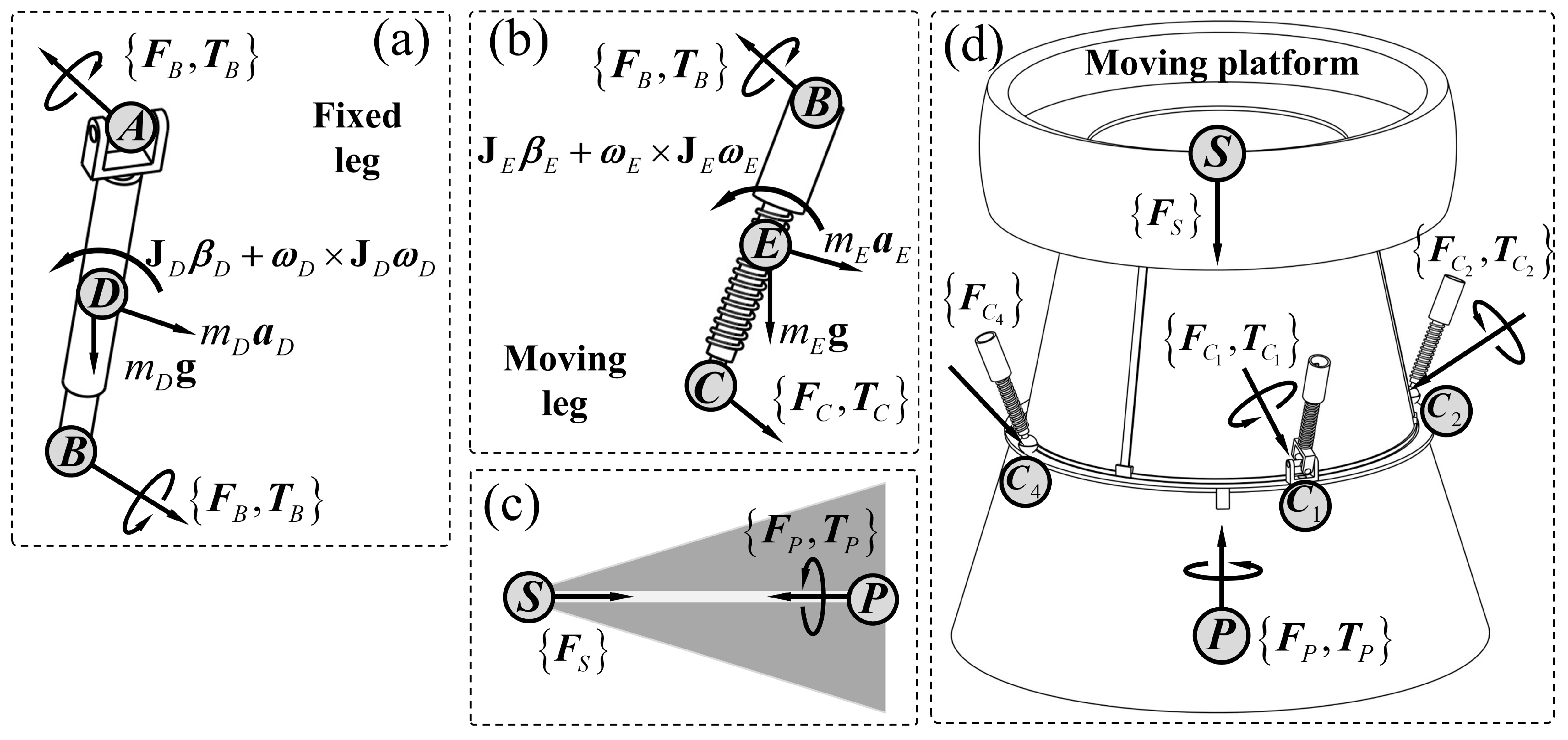
For the $3\mathrm{U}\underset{\_}{\mathrm{P}}\mathrm{S-U}\underset{\_}{\mathrm{P}}\mathrm{U-S}$ parallel mechanism, there are four actuators at the prismatic joints to drive the moving legs, fixed legs and moving platform. As aforementioned in Section 2, the $3\mathrm{U}\underset{\_}{\mathrm{P}}\mathrm{S-U}\underset{\_}{\mathrm{P}}\mathrm{U-S}$ has two rotational degrees of freedom. When it rotates, the inertia force would be generated, and in order to give accurate control, this section will yield the dynamic analysis based on the Newton–Euler equation. The Newton–Euler equation can group all the forces and torques into a single equation. Hence, the three constraint forces and three constraint torques can be calculated in a straightforward way. When the external loads, constraint forces and self-weights of all rigid bodies are considered in the calculation of wrenches, the equation of the balance conditions for a single-rigid-body system is

$$\left[\begin{array}{c}\mathit{F}\\ \mathit{T}\end{array}\right]=\left[\begin{array}{cc}m\mathbf{I}& \mathbf{0}\\ \mathbf{0}& \mathbf{J}\end{array}\right]\left[\begin{array}{c}\mathit{a}\\ \mathsf{\beta }\end{array}\right]+\left[\begin{array}{c}m\mathbf{g}\\ \mathsf{\omega }\times \mathbf{J}\mathsf{\omega }\end{array}\right]$$

(51)

where $\mathit{T}$ is the resultant torque vector, $\mathit{F}$ is the resultant force vector of a single-rigid-body, $\mathbf{I}$ is the 3rd-order identity matrix, and $m$ is the mass of a single-rigid-body at its mass center. $\left\{\mathit{a},\mathsf{\beta }\right\}$ in Equation (51) is the absolute linear acceleration and absolute angular acceleration vector at the mass center according to the absolute coordinate frame, and $\mathsf{\omega }$ is the absolute angular velocity vector at the mass center in the absolute coordinate frame. The acceleration $\left\{\mathit{a},\mathsf{\beta }\right\}$ can be calculated by Equation (50), and the angular velocity $\mathsf{\omega }$ can be obtained using Equation (24).

The moments of inertia $\mathbf{J}$ of a single-rigid-body at its mass center in the absolute coordinate frame (0-coordinate frame) can be obtained through

$$\mathbf{J}={\mathit{R}}_{0n}{\mathbf{J}}_n{\mathit{R}}_{0n}^T$$

(52)

where ${\mathbf{J}}_n$ is the moments of inertia of a single-rigid-body at its mass center in the relative coordinate (n-coordinate frame), and ${\mathit{R}}_{0n}$ is the rotation matrix from the n-coordinate frame to the 0-coordinate frame, which could be calculated by Equation (22).

The fixed leg, $L_{AB}$, has one universal joint and one prismatic joint, which is shown in Figure 4a, and the Newton–Euler equations for the fixed leg, $L_{AB}$, can be derived as

$$\left[\begin{array}{c}{\mathit{F}}_A-{\mathit{F}}_B\\ {}_A\mathit{r}_D\times {\mathit{F}}_A-{}_D\mathit{r}_B\times {\mathit{F}}_B+{\mathit{T}}_A-{\mathit{T}}_B\end{array}\right]=\left[\begin{array}{cc}{m}_D\mathbf{I}& \mathbf{0}\\ \mathbf{0}& {\mathbf{J}}_D\end{array}\right]\left[\begin{array}{c}{\mathit{a}}_D\\ {\mathsf{\beta }}_D\end{array}\right]+\left[\begin{array}{c}{m}_D\mathbf{g}\\ {\mathsf{\omega }}_D\times {\mathbf{J}}_D{\mathsf{\omega }}_D\end{array}\right]$$

(53)

The moving leg, $L_{BC}$, consists of universal joint (or spherical joint) and one prismatic joint, which is shown in Figure 4b, and the Newton–Euler equations for the fixed leg, $L_{BC}$, can be deduced as

$$\left[\begin{array}{c}{\mathit{F}}_B-{\mathit{F}}_C\\ {}_B\mathit{r}_E\times {\mathit{F}}_B-{}_E\mathit{r}_C\times {\mathit{F}}_C+{\mathit{T}}_B-{\mathit{T}}_C\end{array}\right]=\left[\begin{array}{cc}{m}_E\mathbf{I}& \mathbf{0}\\ \mathbf{0}& {\mathbf{J}}_E\end{array}\right]\left[\begin{array}{c}{\mathit{a}}_E\\ {\mathsf{\beta }}_E\end{array}\right]+\left[\begin{array}{c}{m}_E\mathbf{g}\\ {\mathsf{\omega }}_E\times {\mathbf{J}}_E{\mathsf{\omega }}_E\end{array}\right]$$

(54)

When the moving leg, $L_{BC}$, is $\underset{\_}{\mathrm{P}}\mathrm{U}$, the ${\mathbf{T}}_C$ is zero.

The moving platform, $L_P$, consists of one universal joint and four spherical joints, which is shown in Figure 4d. The Newton–Euler equations for the moving platform, $L_P$, can be expressed as

$$\left[\begin{array}{c}{\displaystyle \sum _{k=1}^4{\mathit{F}}_C+{\mathit{F}}_S}\\ {\displaystyle \sum _{k=1}^4\left({}_C\mathit{r}_P\times {\mathit{F}}_C\right)+{\displaystyle \sum _{k=2}^4{\mathit{T}}_C}}\end{array}\right]=\left[\begin{array}{cc}{m}_P\mathbf{I}& \mathbf{0}\\ \mathbf{0}& {\mathbf{J}}_P\end{array}\right]\left[\begin{array}{c}{\mathit{a}}_P\\ {\mathsf{\beta }}_P\end{array}\right]+\left[\begin{array}{c}{m}_P\mathbf{g}\\ {\mathsf{\omega }}_P\times {\mathbf{J}}_P{\mathsf{\omega }}_P\end{array}\right]+\left[\begin{array}{c}{\mathit{F}}_P\\ {\mathit{T}}_P\end{array}\right]$$

(55)

Additionally, the spherical joint at the center has one dimensional constraint equation,

$${\mathit{F}}_S=F_S{\mathit{r}}_S$$

(56)

By associating Equations (53)–(56), the dynamics equation of the $3\mathrm{U}\underset{\_}{\mathrm{P}}\mathrm{S-U}\underset{\_}{\mathrm{P}}\mathrm{U-S}$ parallel mechanism can be derived based on Equation (47):

$$\mathit{c}\mathit{Q}=\mathit{m}\mathit{A}+\mathit{W}+{\mathit{F}}_E$$

(57)

In Equation (57), $\mathit{c}$ is the displacement coefficient matrix for the wrench, $\mathit{Q}$ is the wrench vector consisting of all constraint forces and torques, $\mathit{m}$ is the mass matrix containing mass information of all rigid bodies, $\mathit{A}$ is the acceleration matrix with all acceleration information of each mass center, $\mathit{W}$ is the Coriolis wrench matrix, and ${\mathit{F}}_{\mathit{E}}$ is the external wrench matrix exerted on the $3\mathrm{U}\underset{\_}{\mathrm{P}}\mathrm{S-U}\underset{\_}{\mathrm{P}}\mathrm{U-S}$ parallel mechanism that is given, which also includes gravity.

As shown in Figure 4, the parallel mechanism with the 3$\mathrm{U}\underset{\_}{\mathrm{P}}\mathrm{S}$ chain, 1$\mathrm{U}\underset{\_}{\mathrm{P}}\mathrm{U}$ chain and 1 $\mathrm{S}$ chain has four fixed legs, four moving legs and one moving platform in total. Every single rigid body could establish six equations based on the Newton–Euler equation; therefore, there are 54 equations that could be established.

The universal joint, $\mathrm{U}$, can provide three forces and one torque, the spherical joint can provide three forces and no torque and the prismatic joint can supply three forces and three torques. Therefore, there are 56 unknown constraint forces and torques in the $3\mathrm{U}\underset{\_}{\mathrm{P}}\mathrm{S-U}\underset{\_}{\mathrm{P}}\mathrm{U-S}$ parallel mechanism. As analyzed in Section 2, the $3\mathrm{U}\underset{\_}{\mathrm{P}}\mathrm{S-U}\underset{\_}{\mathrm{P}}\mathrm{U-S}$ is an over constraint parallel mechanism, and a one-dimensional constraint equation at the spherical joint S is added to solve this problem.

The number of constraint wrenches in the $3\mathrm{U}\underset{\_}{\mathrm{P}}\mathrm{S-U}\underset{\_}{\mathrm{P}}\mathrm{U-S}$ parallel mechanism is 56. It is identical to the sum of nonlinear equations in Equations (37)–(39). Therefore, the constraint wrenches can be calculated with Equation (45):

$$\mathit{Q}={\left(\mathit{c}{\mathit{c}}^T\right)}^{-1}\left(\mathit{m}\mathit{A}+\mathit{W}+{\mathit{F}}_E\right)$$

(58)

6. Simulation and Result Analysis

In order to demonstrate the kinematic and dynamic analysis method of the parallel mechanism proposed in this paper, a numerical case is given in this section, and the simulation is carried out by MATLAB software.

6.1. The Inverse Kinematics of the $3\mathrm{U}\underset{\_}{\mathrm{P}}\mathrm{S-U}\underset{\_}{\mathrm{P}}\mathrm{U-S}$ Parallel Mechanism

Suppose that the moving platform follows a spatial rotation motion, and the parameter equation of the trajectory for the moving platform is defined as

$$\{\begin{array}{l}x(t)=-0.2\cos (t)+0.2\\ y(t)=0.1\sin (t)\end{array}$$

(59)

With the trajectory, the displacement vector, ${\mathit{D}}_P$, velocity screw, ${\mathit{V}}_P$ and acceleration vector, ${\mathit{A}}_P$, of the moving platform are

$$\{\begin{array}{l}{\mathit{D}}_P={\left[\begin{array}{cccccc}-0.2\cos (t)+0.2& 0.1\sin (t)& 0& 0& 0& 3\sqrt{3}/10\end{array}\right]}^T\\ {\mathit{V}}_P={\left[\begin{array}{cccccc}0.2\sin (t)& 0.1\cos (t)& 0& 0& 0& 0\end{array}\right]}^T\\ {\mathit{A}}_P={\left[\begin{array}{cccccc}0.2\cos (t)+0.2& 0.1\sin (t)& 0& 0& 0& 0\end{array}\right]}^T\end{array}$$

(60)

where $t$ is the time of the trajectory.

The step length for simulation is $\Delta t=0.001$, and the total number of iterations is $n=10000$. As illustrated in Figure 5, $H\left(\mathrm{m}\right)$ is the initial height between the mass center, $S$, on the base platform and the mass center, $P$, of the moving platform, $L\left(\mathrm{m}\right)$ is the initial length between joint $A$ and joint $C$. $R\left(\mathrm{m}\right)$ is the distance between the mass center $S$ and joint $A$, $r\left(\mathrm{m}\right)$ is the distance between the mass center $P$ and joint $C$, and both are constant. $\theta$ and $P$ give the initial assembly configuration of four surrounding kinematic chains. The initial configuration conditions of the $3\mathrm{U}\underset{\_}{\mathrm{P}}\mathrm{S-U}\underset{\_}{\mathrm{P}}\mathrm{U-S}$ parallel mechanism for kinematics analysis is given in

Table 1. Structure parameters of the $3\mathrm{U}\mathrm{P}\mathrm{S-U}\mathrm{P}\mathrm{U-S}$.

$H\left(\mathrm{m}\right),\left(t=0\right)$	$R\left(\mathrm{m}\right)$	$r\left(\mathrm{m}\right)$	$L\left(\mathrm{m}\right),\left(t=0\right)$
$\frac{3\sqrt{3}}{10}$	$0.8$	$0.5$	$0.6$

and

Table 2. Initial conditions of the $3\mathrm{U}\mathrm{P}\mathrm{S-U}\mathrm{P}\mathrm{U-S}$.

${\theta }_1^i\left(0\right)\left(\mathrm{rad}\right)$	${\theta }_2^i\left(0\right)\left(\mathrm{rad}\right)$	$p_3^i\left(0\right)\left(\mathrm{m}\right)$	${\theta }_4^i\left(0\right)\left(\mathrm{rad}\right)$	${\theta }_5^i\left(0\right)\left(\mathrm{rad}\right)$	${\theta }_6^i\left(0\right)\left(\mathrm{rad}\right)$
$\left\{{\theta }_1^1\right\}=\left\{0\right\}$	$\left\{{\theta }_2^1\right\}=\left\{-\frac{\pi }{6}\right\}$	$\left\{p_3^1\right\}=\left\{0.3\right\}$	$\left\{{\theta }_4^1\right\}=\left\{0\right\}$	$\left\{{\theta }_5^1\right\}=\left\{-\frac{\pi }{3}\right\}$	$\left\{{\theta }_6^1\right\}=\left\{0\right\}$

.

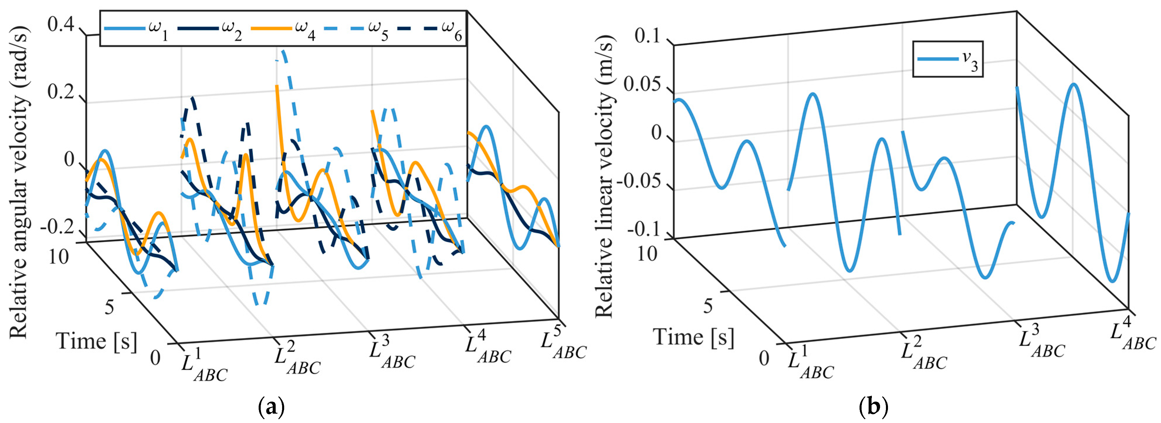
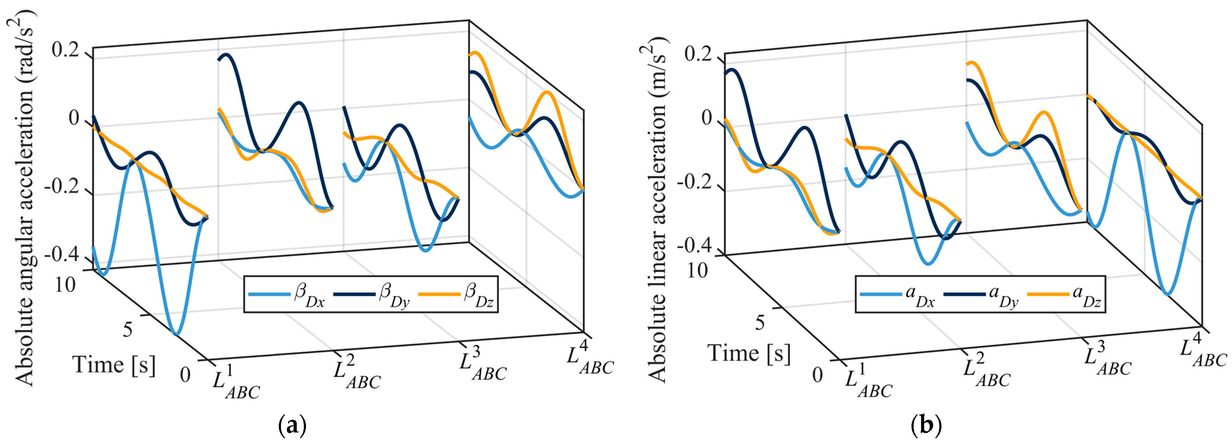
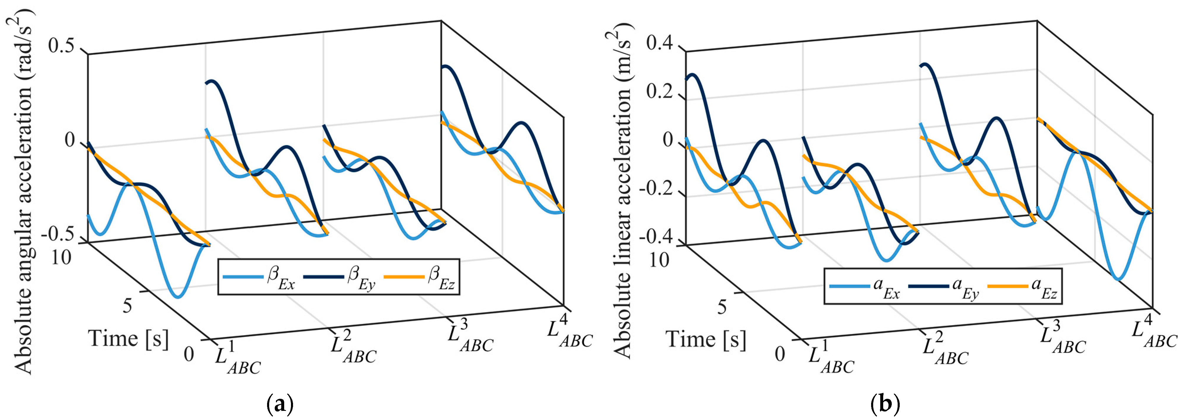
Starting from the initial configuration, the kinematics of the $3\mathrm{U}\underset{\_}{\mathrm{P}}\mathrm{S-U}\underset{\_}{\mathrm{P}}\mathrm{U-S}$ $3\mathrm{U}\underset{\_}{\mathrm{P}}\mathrm{S-U}\underset{\_}{\mathrm{P}}\mathrm{U-S}$ parallel mechanism could be calculated, the angular velocities could be derived by Equation (24), the postures and positions could be derived by Equation (22) and the accelerations could be derived by Equations (44) and (50). The inverse kinematics of the $3\mathrm{U}\underset{\_}{\mathrm{P}}\mathrm{S-U}\underset{\_}{\mathrm{P}}\mathrm{U-S}$ parallel mechanism is carried out and plotted by MATLAB based on the given trajectory, and the curves of the kinematics are shown in Figure 6, Figure 7, Figure 8, Figure 9 and Figure 10. In Figure 8, Figure 9 and Figure 10, the subscripts $x,y,z$ represent the components around the coordinate axis, respectively.

Figure 6 shows the relative angular displacements and relative linear displacements of all the joints in each kinematic chain. Figure 6a illustrates the relative angular displacement $\theta$ of all the revolute joints of each kinematic chain, and Figure 6b illustrates the relative linear displacements $d$ of all prismatic joints.

Figure 7 represents the relative angular velocities and relative linear velocities of all the joints in each kinematic chain. Figure 7a shows the relative angular velocities $\omega$ of each rotational joint, and Figure 7b shows the relative linear velocities $v_3$ of each prismatic joint.

Figure 8 depicts the absolute angular accelerations and absolute angular accelerations of the mass center $D$ of the fixed leg $L_{AB}^K,\left(K=1,2,3,4\right)$ in each kinematic chain; the $\beta$ is the absolute angular accelerations and the a is the absolute linear acceleration.

Figure 9 shows the absolute angular accelerations and absolute angular accelerations of the moving legs, $L_{BC}^K,\left(K=1,2,3,4\right)$, at their individual mass centers $E$. Figure 9a shows the absolute angular accelerations, and Figure 9b shows the absolute linear acceleration.

Figure 10 illustrates the absolute angular velocities of all chains. Figure 10a shows the absolute angular velocities of the fixed legs at their mass center $D$ of each chain and Figure 10b shows the absolute angular velocities of the mass center $E$ of each moving leg.

6.2. The Inverse Dynamics of the $3\mathrm{U}\underset{\_}{\mathrm{P}}\mathrm{S-U}\underset{\_}{\mathrm{P}}\mathrm{U-S}$ Parallel Mechanism

Assume that there are external loads exerting on the moving platform at its mass center $P$ given the external force ${\mathit{F}}_P=\left[\begin{array}{ccc}0& 0& 1\end{array}\right]\left(\mathrm{K}\mathrm{N}\right)$ and the torque ${\mathit{T}}_P=\left[\begin{array}{ccc}1& 0& 0\end{array}\right]\left(\mathrm{K}\mathrm{N}\cdot \mathrm{m}\right)$. With the kinematics information calculated in Section 6.1, and the identified inertial parameters at mass’ center and moving platform in

Table 3. The identified inertial parameters at mass center and moving platform.

Mass $\left(\mathrm{m}\right)\left(K=1,2\cdots 4\right)$	Moments of inertia $\left(\mathrm{kg}\cdot {\mathrm{m}}^2\right)\left(K=1,2\cdots 4\right)$
$\{\begin{array}{l}{m}_D^K=1.42 \mathrm{k}\mathrm{g}\\ m_E^K=1.42 \mathrm{k}\mathrm{g}\\ m_P=2.87 \mathrm{k}\mathrm{g}\end{array}$	$\{\begin{array}{l}{\mathbf{J}}_{D_0}^K=\left[\begin{array}{ccc}5.56e^{-4}& 0& 0\\ 0& 1.14e^{-2}& 0\\ 0& 0& 1.16e^{-2}\end{array}\right]={\mathbf{J}}_{E_0}^K\\ {\mathbf{J}}_{P_0}=\left[\begin{array}{ccc}6.87e^{-1}& 0& 0\\ 0& 6.87e^{-1}& 0\\ 0& 0& 9.21e^{-1}\end{array}\right]\end{array}$

, the dynamics analysis of the $3\mathrm{U}\underset{\_}{\mathrm{P}}\mathrm{S-U}\underset{\_}{\mathrm{P}}\mathrm{U-S}$ parallel mechanism could be carried out, and the driving force of the prismatic joint could be derived using Equation (56).

Figure 11 depicts the resultant driving forces at all prismatic joints of the four kinematic chains. In addition, the component forces along three coordinate frames can be derived with the direction of each chain, and the curves indicate that the resulting driving forces are varied as the motion of the moving platform changes.

7. Conclusions

This paper proposes an $3\mathrm{U}\underset{\_}{\mathrm{P}}\mathrm{S-U}\underset{\_}{\mathrm{P}}\mathrm{U-S}$ over constraint parallel mechanism to satisfy the motion demands of two rotational degrees of freedom. The kinematics and dynamics based on screw theory are investigated. Different to the existing methods, the most prominent merits of this method are that the displacements, velocities, position and postures are calculated by the velocity screw equation directly and the acceleration in screw form is given; therefore, this mathematical expression could simplify the calculation and analysis of the dynamics. Both forces and torques could be taken into account in the equilibrium of the parallel mechanism, and all the constraint forces and torques could be calculated in the absolute coordinate system. The kinematics and dynamics could be united by using the unit screw matrix. This method could also be applied to develop the program to analyze the kinematics and dynamics of any other multi-rigid-body system. The workspace and trajectory planning could be discussed for application in future work.

References

- Wu, J.; Chen, X.; Wang, L.; Liu, X. Dynamic load-carrying capacity of a novel redundantly actuated parallel conveyor. Nonlinear Dyn. 2014, 78, 241–250. [Google Scholar] [CrossRef]
- Jamwal, P.K.; Xie, S.Q.; Tsoi, Y.H.; Aw, K.C. Forward kinematics modelling of a parallel ankle rehabilitation robot using modified fuzzy inference. Mech. Mach. Theory 2010, 45, 1537–1554. [Google Scholar] [CrossRef]
- Zhao, J.; Zhou, K.; Mao, D.; Gao, Y.; Fang, Y. A new method to study the degree of freedom of spatial parallel mechanisms. Int. J. Adv. Manuf. Technol. 2004, 23, 288–294. [Google Scholar] [CrossRef]
- Zhao, J.; Zhou, K.; Feng, Z. A theory of degrees of freedom for mechanisms. Mech. Mach. Theory 2004, 39, 621–643. [Google Scholar] [CrossRef]
- Kelaiaia, R.; Zaatri, A.; Company, O. Multiobjective Optimization of 6-dof UPS Parallel Manipulators. Adv. Robot. 2012, 26, 1885–1913. [Google Scholar] [CrossRef]
- Peng, B.; Li, Z.; Wu, K.; Sun, Y. Kinematic Characteristics of 3-UPU Parallel Manipulator in Singularity and Its Application. Int. J. Adv. Robot. Syst. 2011, 8, 54–64. [Google Scholar]
- Lazic, D.V.; Ristanovic, M.R. Electrohydraulic thrust vector control of twin rocket engines with position feedback via angular transducers. Control. Eng. Pract. 2007, 15, 583–594. [Google Scholar] [CrossRef]
- Rosyid, A.; El-Khasawneh, B. Multibody Dynamics of Nonsymmetric Planar 3PRR Parallel Manipulator with Fully Flexible Links. Appl. Sci. 2020, 10, 4816. [Google Scholar] [CrossRef]
- Brahmia, A.; Kelaiaia, R.; Chemori, A.; Company, O. On Robust Mechanical Design of PAR2 Delta-Like Parallel Kinematic Manipulator. J. Mech. Robot. 2022, 14, 011001. [Google Scholar] [CrossRef]
- Gallardo-Alvarado, J.; Aguilar-Nájera, C.R.; Casique-Rosas, L.; Pérez-González, L.; Rico-Martínez, J.M. Solving the kinematics and dynamics of a modular spatial hyper-redundant manipulator by means of Plücker coordinate. Multibody Syst. Dyn. 2008, 20, 307–325. [Google Scholar] [CrossRef]
- Gan, D.; Liao, Q.; Wang, P. Forward Kinematics Analysis and Motion Simulation of a New 6-CCS Parallel Mechanism. China Mech. Eng. 2007, 18, 2903–2906. [Google Scholar]
- Shao, B.; Yuan, E. An United Recursive Robot Dynamics Based on Screws. AASRI Procedia 2012, 3, 54–59. [Google Scholar] [CrossRef]
- Nurahmi, L.; Gan, D. Dynamic Analysis of the 3-RRPS Metamorphic Parallel Mechanism Based on Instantaneous Screw Axis. In Proceedings of the ASME 2019 International Design Engineering Technical Conferences and Computers and Information in Engineering Conference, 2019, 5A: 43rd Mechanisms and Robotics Conference, Anaheim, CA, USA, 18–21 August 2019. [Google Scholar]
- Cardozo, W.S.; Weber, H.I. Dynamic modeling of a 2-dof parallel electrohydraulic-actuated homokinetic platform. Mech. Mach. Theory 2017, 118, 1–13. [Google Scholar] [CrossRef]
- Dasgupta, B.; Choudhury, P. A general strategy based on the Newton-Euler approach for the dynamic formulation of parallel manipulators. Mech. Mach. Theory 1999, 34, 801–824. [Google Scholar] [CrossRef]
- Chen, X.; Wu, L.; Deng, Y.; Wang, Q. Dynamic response analysis and chaos identification of 4-UPS-UPU flexible spatial parallel mechanism. Nonlinear Dyn. 2017, 87, 2311–2324. [Google Scholar] [CrossRef]
- Abdellatif, H.; Heimann, B. Computational efficient inverse dynamics of 6-DoF fully parallel manipulators by using the Lagrangian formalism. Mech. Mach. Theory 2009, 44, 192–207. [Google Scholar] [CrossRef]
- Liu, S.; Peng, G.; Gao, H. Dynamic modeling and terminal sliding mode control of a 3-DoF redundantly actuated parallel platform. Mechatronics 2019, 60, 26–33. [Google Scholar] [CrossRef]
- Chen, M.; Zhang, Q.; Qin, X.; Sun, Y. Kinematic, dynamic, and performance analysis of a new 3-DoF over-constrained parallel mechanism without parasitic motion. Mech. Mach. Theory 2021, 162, 104365. [Google Scholar] [CrossRef]
- Merlet, J.P.; Gosselin, C. Parallel Mechanisms and Robots; Springer Handbook of Robotics: Berlin/Heidelberg, Germany, 2008; pp. 269–285. [Google Scholar]
- Ren, J.; Cao, Q. Dynamic Modeling and Frequency Characteristic Analysis of a Novel 3-PSS Flexible Parallel Micro-Manipulator. Micromachines 2021, 12, 678. [Google Scholar] [CrossRef]
- Ren, J.; Li, Q.; Wu, H.; Cao, Q. Optimal Design for 3-PSS Flexible Parallel Micromanipulator Based on Kinematic and Dynamic Characteristics. Micromachines 2022, 13, 1457. [Google Scholar] [CrossRef]
- Rosyid, A.; El-Khasawneh, B. Identification of the Dynamic Parameters of a Parallel Kinematics Mechanism with Prismatic Joints by Considering Varying Friction. Appl. Sci. 2020, 10, 4820. [Google Scholar] [CrossRef]
- Hu, B.; Yu, J.; Lu, Y. Inverse dynamics modeling of a (3-UPU) (3-UPS S) serial-parallel manipulator. Robotica 2016, 34, 687–702. [Google Scholar] [CrossRef]
- Niu, A.; Wang, S.; Sun, Y.; Qiu, J.; Qiu, W.; Chen, H. Dynamic modeling and analysis of a novel offshore gangway with 3UPU/UP-RRP series-parallel hybrid structure. Ocean. Eng. 2022, 266, 113122. [Google Scholar] [CrossRef]
- Safeea, M.; Neto, P.; Bearee, R. Robot dynamics: A recursive algorithm for efficient calculation of Christoffel symbols. Mech. Mach. Theory 2019, 142, 103589. [Google Scholar] [CrossRef] [Green Version]
- Hudgens, J.C.; Tesar, D. Analysis of a Fully-Parallel Six Degree-of-Freedom Micromanipulator. In Proceedings of the Fifth International Conference on Advanced Robotics ’Robots in Unstructured Environments, Pisa, Italy, 19–22 June 1991. [Google Scholar]
- Liu, M.; Li, C.; Li, C. Dynamics analysis of the gough-stewart platform manipulator. IEEE Trans. Robot. Autom. 2000, 16, 94–98. [Google Scholar]
- Yun, Y.; Li, Y. A general dynamics and control model of a class of multi-DoF manipulators for active vibration control. Mech. Mach. Theory 2011, 46, 1549–1574. [Google Scholar] [CrossRef]
- Wen, S.; Qin, G.; Zhang, B.; Lam, H.; Zhan, Y.; Wang, H. The study of model predictive control algorithm based on the force/position control scheme of the 5-DoF redundant actuation parallel robot. Robot. Auton. Syst. 2016, 79, 12–25. [Google Scholar] [CrossRef] [Green Version]
- Jiao, J.; Wu, Y.; Yu, K.; Zhao, R. Dynamic modeling and experimental analyses of Stewart platform with flexible hinges. J. Vib. Control. 2019, 25, 151–171. [Google Scholar] [CrossRef]
- Gallardo-Alvarado, J.; Rico, J.M.; Frisoli, A.; Checcacci, D.; Bergamasco, M. Dynamics of parallel manipulators by means of screw theory. Mech. Mach. Theory 2003, 38, 1113–1131. [Google Scholar] [CrossRef]
- Gallardo-Alvarado, J.; Rico, J.M.; Delossantos-Lara, P.J. Kinematics and dynamics of a 4- PRUR Schönflies parallel manipulator by means of screw theory and the principle of virtual work. Mech. Mach. Theory 2018, 122, 347–360. [Google Scholar] [CrossRef]
- Liu, Z.; Tao, R.; Fan, J.; Wang, Z.; Jing, F.; Tan, M. Kinematics, dynamics, and load distribution analysis of a 4-PPPS redundantly actuated parallel manipulator. Mech. Mach. Theory 2022, 167, 104494. [Google Scholar] [CrossRef]
- Garcia-Murillo, M.A.; Sanchez-Alonso, R.E.; Gallardo-Alvarado, J. Kinematics and Dynamics of a Translational Parallel Robot Based on Planar Mechanisms. Machines 2016, 4, 22. [Google Scholar] [CrossRef] [Green Version]
Figure 1.
Geometry of the parallel mechanism: (a) front view; (b) top view of the parallel mechanism.
Figure 2.
Kinematics of the parallel mechanism: (a) kinematics of the chain; (b) kinematics of the chain; (c) kinematics of the chain.
Figure 3.
Acceleration analysis of multi-rigid body system.
Figure 4.
Dynamics of the parallel mechanism: (a) dynamics of the fixed leg ; (b) dynamics of the moving leg ; (c) dynamics of the chain; (d) dynamics of the moving platform.
Figure 5.
Initial configuration of the parallel mechanism.
Figure 6.
Relative angular displacements and relative linear displacements of each joint: (a) relative angular displacements; (b) relative linear displacements.
Figure 7.
Relative angular velocities and relative linear velocities of each joint: (a) relative angular velocities; (b) relative linear velocities.
Figure 8.
Absolute angular accelerations and absolute linear accelerations of fixed legs, at their respective mass centers : (a) absolute angular accelerations; (b) absolute linear accelerations.
Figure 9.
Absolute angular accelerations and linear accelerations of moving legs at their respective mass centers : (a) absolute angular accelerations; (b) absolute linear accelerations.
Figure 10.
Absolute angular velocities of the mass centers, and , of all legs: (a) absolute angular velocities of the fixed legs, ; (b) absolute angular velocities of the moving legs, .
Figure 11.
The driving forces of the prismatic joint in the parallel mechanism.